Bayesian reconstruction of sea level and hydroclimates from coastal landform inversion: application to Santa Cruz (US) and Gulf of Corinth

Quantifying Quaternary sea-level changes and hydroclimatic conditions is an important challenge, given their intricate relation with paleo-climate, ice-sheets, and geodynamics. The world's coastlines provide an enormous geomorphologic archive, from which forward landscape evolution modeling studies have shown their potential to unravel paleo sea levels, albeit at the cost of assumptions on the genesis of these landforms. We take a next step, by applying a Bayesian approach to jointly invert the geometries of multiple coastal terrace sequences to paleo sea- and lake-level variations and extract past hydroclimatic conditions. Using a Markov chain Monte Carlo sampling method, we first test our approach on synthetic marine terrace profiles as proof of concept and then benchmark our model on an observed marine terrace sequence in Santa Cruz (US). We successfully reproduce observed sequence morphologies and simultaneously obtain probabilistic estimates for past sea-level variations, as well as for other model parameters, such as uplift and erosion rates. When applied to the semi-isolated Gulf of Corinth (Greece), our method allows the geomorphic Rosetta stone to be deciphered at an unprecedented resolution, revealing the connectivity between the Lake/Gulf of Corinth and the open sea for different hydroclimatic conditions. Eustatic sea levels and changing sill depths drive marine and transitional phases during interglacial and interstadial periods, whereas wetter and drier hydroclimates, respectively, over- and underfill Lake Corinth during interstadial and glacial periods.

1 Introduction

Reconstructions of Quaternary sea-level variations provide crucial constraints on thresholds and feedbacks within climatic and geodynamic systems that help understand how contemporary climate change may affect future sea levels (Lambeck and Chappell, 2001; Hay et al., 2014; Dutton et al., 2015; Shakun et al.,. 2015; Austermann et al.,. 2017). A key archive of past sea levels is exposed within the geomorphology of most of the world's coastal areas, in the form of paleo shorelines (Johnson and Libbey, 1997; Pedoja et al., 2011, 2014; Rovere et al., 2023; Fig. 1a), but it remains difficult to accurately translate coastal observations and measurements into paleo sea-level estimates and to evaluate the uncertainties inherent to these conversions. Major challenges include (1) dating of these landforms, as most paleo-shorelines are erosive in nature (Pedoja et al., 2014) and absolute dating techniques themselves are complex and prone to large uncertainties (Strobl et al., 2014; Hibbert et al., 2016; Ott et al., 2019); (2) observational bias, which is mostly restricted to the most recent glacial cycle(s) and to periods where relative sea levels were at similar elevations to the present day (Medina-Elizalde, 2013; Hibbert et al., 2016); (3) the absence of reciprocity between paleo-shorelines and sea-level stands, as not all highstands lead to paleo-shorelines and paleo-shorelines may have formed during one or many sea-level cycles (Guilcher, 1974; Malatesta et al., 2022; Chauveau et al., 2024); and (4) separating the tectonic from the sea-level component within relative sea-level changes (Pedoja et al., 2011).

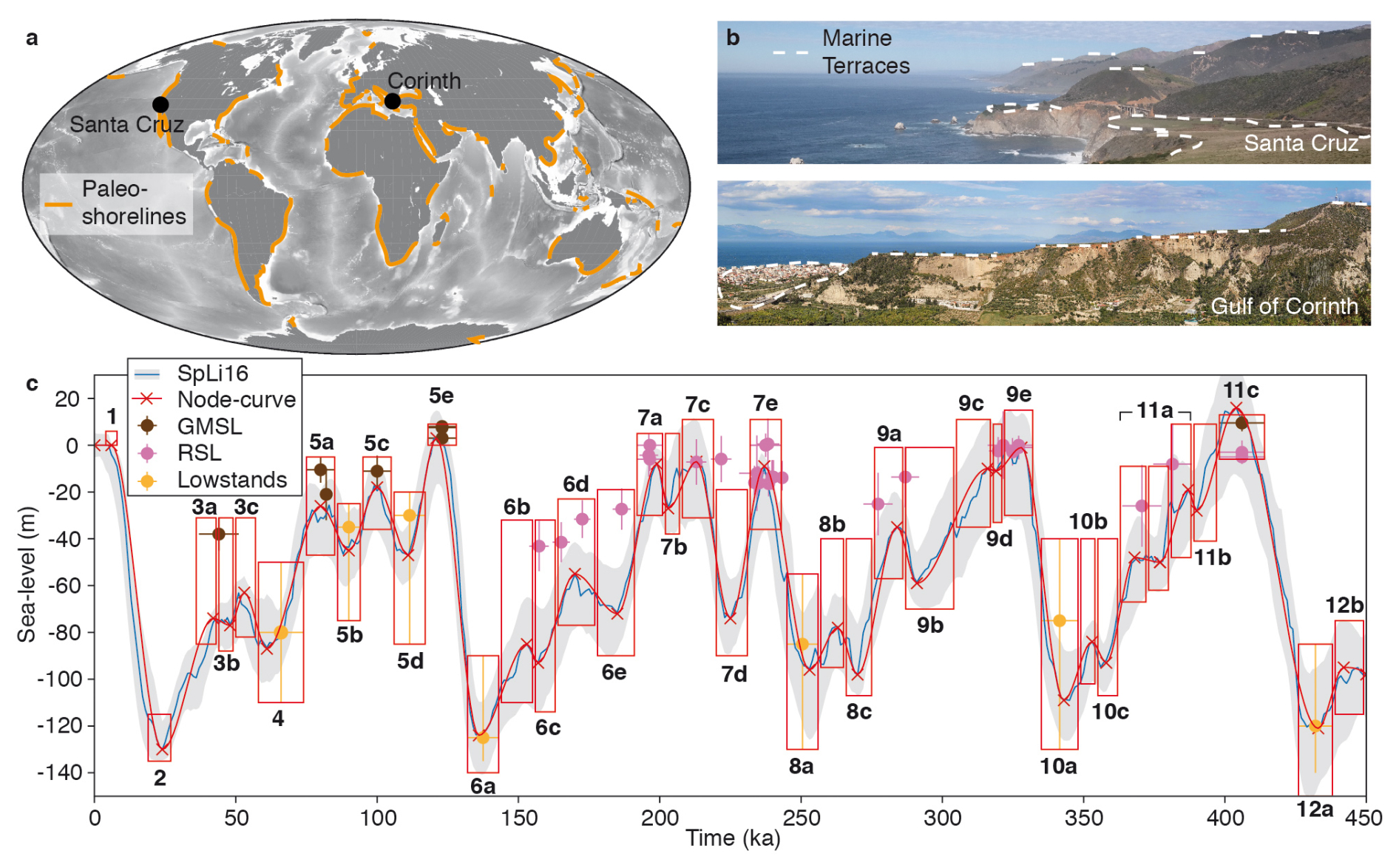
Figure 1 Paleo-shorelines and paleo sea level. (a) Global compilation of paleo-shoreline sequences, adjusted from Pedoja et al. (2014). (b) Marine terrace sequences from Santa Cruz (US) and the Corinth Rift (Greece). (c) Paleo sea-level estimates for the past 450 ka, showing a sea-level curve (SpLi16, blue; Spratt and Lisiecki, 2016) derived from principal component analysis of seven sea-level curves, with its 2.5 % and 97.5 % likelihood range (gray envelope), an approximation of that curve with nodes and a cubic spline interpolation (red), global mean sea-level highstand estimates adjusted for glacio-isostatic adjustments (GMSL, brown dots; Kopp et al., 2009; Dutton et al., 2015; Pico et al., 2016; Creveling et al., 2017; Dyer et al., 2021; Tawil-Morsink et al., 2022), selected relative sea-level highstand estimates >130 ka (RSL, pink dots; Stirling et al., 2001; Murray-Wallace, 2002; Andersen et al., 2010; de Gelder et al., 2022; Marra et al., 2023), global mean sea-level lowstand estimates from ice sheet data (orange dots; Batchelor et al., 2019), and red boxes that represent the likely admissible range of relative sea-level elevations at locations far from the major ice-sheets (details in the Supplement and Table S1) that we consider in this study. Marine isotope stages (MISs), given in bold, are based on Railsback et al. (2015).

Numerical models of landscape evolution started to overcome some of these limitations, by providing a means to quantitatively interpret undated paleo-shorelines, incorporating full sea-level curves instead of highstands only, unraveling the creation of paleo-shorelines formed over multiple glacial cycles, and considering multiple sea-level curves (e.g., Webster et al., 2007; Jara-Muñoz et al., 2019; Leclerc and Feuillet, 2019; de Gelder et al., 2020; 2023). So far, such numerical models have mainly been used for forward modeling approaches, where a number of proposed sea-level curves are used to predict shorelines, which are then compared with actual observations. However, this only provides a limited way to explore the full ensemble of possible sea-level histories and other model parameters, like rock erosion rates or effective wave-base depths, which are difficult to estimate. It follows that uncertainties in sea-level estimates from marine terraces remain poorly known, regardless of the method used and in spite of uniformization attempts (Lorscheid and Rovere, 2019).

Semi-isolated marine basins, i.e., bodies of water that have been connected to the open sea in some intervals of their geologic history and little connected or disconnected from the sea in other intervals, develop in hydrodynamic settings for which it is particularly complex to reconstruct sea and lake levels. Such basins, like the Red Sea, Sea of Marmara (Türkiye), Cariaco Basin (Venezuela), and Gulf of Corinth (Greece), have a special geologic interest, given the active tectono-sedimentary processes driving their formation (e.g., Van Daele et al., 2011; McNeill et al., 2019), their sensitivity to rapid sea-level and climatic changes (e.g., Aksu et al., 1999; Siddall et al., 2004), and their role in dispersion of species (e.g., Derricourt, 2005). The main complexity in reconstructing sea-/lake-level fluctuations in such settings is that (1) during disconnected phases these basins may have been underfilled or overfilled, depending on the local hydroclimate, and (2) the structural highs (sills) separating the basins from the sea can be simultaneously affected by tectonic vertical motion, sedimentation, and erosion.

In this study, we intend to overcome common marine terrace analysis limitations by using a Bayesian approach to invert the geometry of paleo-shoreline sequences. Our approach provides probabilistic estimates of paleo sea level, erosion rates, uplift rates, wave-base depths, and initial slopes. We focus on erosive marine terraces (Fig. 1b), which are both the most common type of paleo-shoreline (Pedoja et al., 2014) and simpler to model than their depositional and bio-constructed equivalents (e.g., Pastier et al., 2019). We first apply our probabilistic inversion approach to a set of synthetic coastal profiles to test and illustrate the method, after which we invert a well-studied marine terrace sequence in Santa Cruz (US) to benchmark our model on a natural example. Finally, we use our approach on the semi-isolated Gulf of Corinth to decipher the complex combination of tectonic uplift, sea- and lake-level fluctuations, local climatic drivers, and sill dynamics. The Gulf of Corinth has been considered a natural rift laboratory and has therefore received a lot of attention as a primary example for studying tectonic and surface processes in young rift systems (e.g., Armijo et al., 1996; Bernard et al., 2006; Nixon et al., 2016; Gallen and Fernández-Blanco, 2021). As a semi-isolated marine basin, it has also been subjected to many studies on its environmental and climatic evolution (e.g., Collier et al., 2000; Watkins et al., 2019) yet, so far, previous studies could not resolve to what extent sea and lake levels have fluctuated.

These case studies highlight how we can derive probabilistic estimates of past sea levels from marine terraces and how the natural archive of paleo-shorelines can be further utilized to both improve paleo sea-level estimates and unravel complex tectono-hydroclimatic interactions.

2 Marine terrace sequence inversion

Marine terraces are relatively flat surfaces of coastal origin, either horizontal or gently inclined seaward (Fig. 1b; Pirazzoli, 2005). They are bounded inland by a fossil sea-cliff and can be covered by a layer of coastal sediments. Here we model erosive marine terraces, which are primarily formed by sea-cliff retreat in response to wave action. The superposition of Quaternary sea-level variations (Fig. 1c) and vertical land movement typically leads to a staircase landscape exhibiting marine terrace sequences (Fig. 1b). In the following sub-sections, we describe the inversion of marine terraces in four parts: (1) the unknown model parameters and their relation to observed terraces, (2) the Bayesian formulation of the inverse problem, (3) the Monte Carlo algorithm to approximate the probabilistic solution, and (4) the bounds of the uniform prior ranges.

2.1 Model parameters

As a general formulation, we can consider

$$\begin{array}{}\text{(1)}& \mathit{d}=g\left(m\right)+\mathit{\epsilon },\end{array}$$

where d is the vector of observations, in our case the topographic profile of a terrace sequence, and m is the set of unknown model parameters to be inverted for: uplift rate (U), erosion rate (E^∗), wave-base depth (z₀), initial slope (α), and sea-level history, described by a set of nodes (see the following). The function g describes the numerical erosion model that links these model parameters to the topographic profile, here the REEF code (Husson et al., 2018; Pastier et al., 2019). Data errors here are given by a random variable ε that describes the inability of the forward model g(m) to explain the observations d.

REEF is a nonlinear model, in which wave erosion is based on the wave energy dissipation model developed by Anderson et al. (1999). The model assumes that the vertical seabed erosion rate is a linear function of the rate of wave energy dissipation against the seabed (Sunamura, 1992). Horizontal erosion rates depend on the energy available at the sea-cliff after dissipation of the far-field wave energy (Anderson et al., 1999). The dissipation rate is dictated by the water depth profile, which increases landward exponentially with decreasing water depth. The initial erosion rate E^∗ is expressed as an effective eroded volume per unit of time and coastal length, in which a fraction of erosional residual power E_r erodes the foundation at each location along the curvilinear profile s. This fraction E_r depends on the true local water depth along the profile h(s), the water depth for wave-base erosion z₀, and a coefficient for sea bed erodibility K, so that

$$\begin{array}{}\text{(2)}& {\displaystyle \frac{\partial E_{\mathrm{r}}}{\partial t}}=K\times E_{\mathrm{r}}\times \exp \left(-{\displaystyle \frac{h\left(s\right)}{z_{\mathrm{0}}}}\right).\end{array}$$

Then a residual power $E^{\ast }-{\int }_s(\partial E_{\mathrm{r}}/\partial t)\mathrm{d}s$ carves out a 1 m high notch and all its overhanging material to form a cliff. Following previous studies (Anderson et al., 1999; Pastier et al., 2019), for K we use 0.1 as bedrock erodibility and 1 for notch carving. Finally, the 2D model we use consists of a landmass with a seaward dipping linear initial slope (α; Fig. 2a), an initial erosion rate (E^∗; Fig. 2a) that evolves as platforms are being carved, a wave-base depth (z₀; Fig. 2a) that determines the vertical range over which erosion takes place, a land uplift rate (U; Fig. 2a), and a sea-level history.

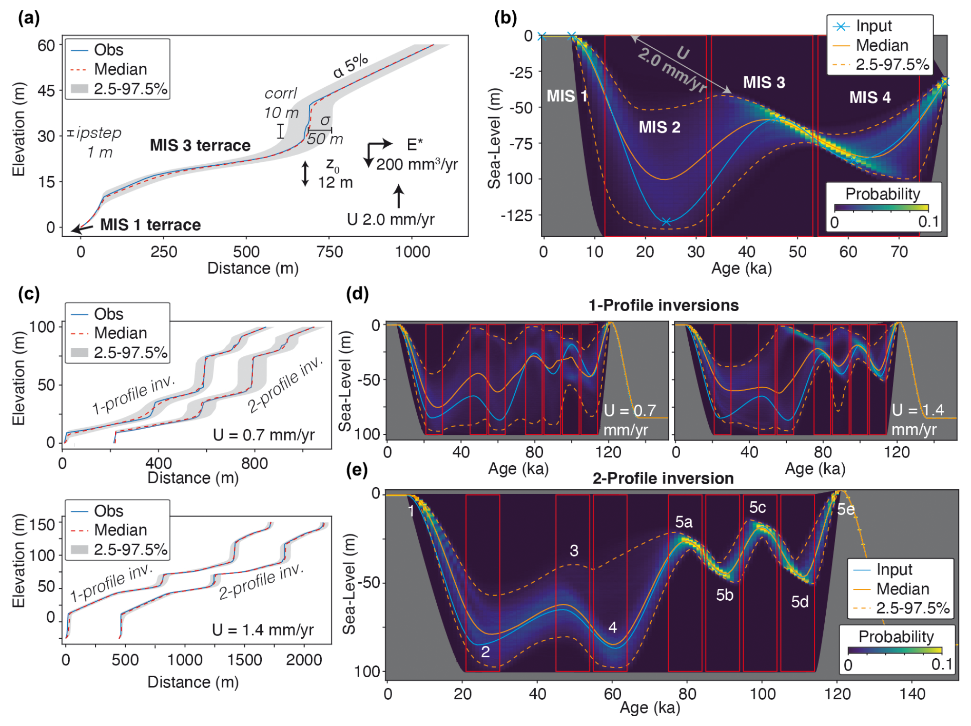
Figure 2 Inversion of synthetic marine terrace profiles. (a) Synthetic topography (Obs, blue) created from a forward model with known input parameters: α = initial slope, E^∗ = erosion rate, U = uplift rate, and z₀ = wave-base depth. The posterior range of models that fit the observed topography with the given σ, ipstep, and corrl (see text) is represented by the median (orange), and the 2.5 and 97.5 percentiles of the inverted models (gray envelope). (b) Posterior probability distribution for the sea-level histories. Each individual paleo sea-level history is described with six sea-level nodes linked with a cubic spline interpolation, of which the nodes at 78, 6, and 0 ka are fixed in time and elevation and the other three nodes can move within the three red boxes. The input (target) sea-level history is given in light blue and the probabilistic solution is depicted by the median (solid orange line) and the 2.5 and 97.5 percentiles (dashed orange lines). (c) Same as (a), but with different uplift rates and sea-level histories. (d) Sea-level histories for the inverted profiles in (c), similar to (b) but with a different input sea-level history, including more nodes. (e) Similar to (b), but inverting the two profiles simultaneously to find a common sea-level curve explaining both profiles. MISs are marked in white.

To invert the morphology of the marine terrace sequences, we parameterize sea-level history (sl) with a finite number of unknown parameters. We use nodes interpolated through a cubic spline scheme (Fig. 2b; light blue), in which each node has values for age and elevation.

This creates sea-level curves with similar characteristics to published sea-level curves (red line, Fig. 1c), in which the nodes represent sea-level minima (lowstands) and maxima (highstands) that are typically linked to even- and odd-numbered marine isotope stages (MISs), respectively.

2.2 Bayesian formulation of the inverse problem

Reconstructing the sea-level history from present-day observations of marine terrace sequences can be mathematically formulated as a highly nonlinear inverse problem where the solution is nonunique. To embrace this nonuniqueness, the problem can be cast in a Bayesian (probabilistic) framework where the solution is a posterior probability distribution describing the probability of the model parameters (m), given the observed data (d).

One benefit of Bayesian inference is the ability to propagate uncertainty estimates from the observed measurements (ε in Eq. 1) toward the unknown model parameters. For that, a likelihood probability distribution needs to be defined, based on the mathematical model for uncertainty estimates associated with observations. The errors ε about the observed shorelines account for the inability of our numerical model g(m) to explain observations d and can be due to both observational (either instrumental or due to a naturally degrading morphology) or modeling errors. These errors are supposedly random and normally distributed. Their statistics can therefore be described by a covariance matrix C_d defined by a standard deviation (σ; Fig. 2a) and a level of spatial correlation (corrl; Fig. 2a). In this way, the likelihood distribution defining the probability of observing the data d, given a set of model parameters m, is written as

$$\begin{array}{}\text{(3)}& p\left(\mathit{d}\mathrm{|}m\right)\propto \exp \left(-{\displaystyle \frac{\mathrm{1}}{\mathrm{2}}}{\left[\mathit{d}-g\left(m\right)\right]}^{\mathrm{T}}{\mathbf{C}}_{\mathit{d}}^{-\mathrm{1}}\left[\mathit{d}-g\left(m\right)\right]\right).\end{array}$$

In order to probabilistically estimate the model parameters, Bayes' theorem can be used to combine this likelihood distribution (information given by the data), with the prior distribution p(m) that represents independent information on model parameters:

$$\begin{array}{}\text{(4)}& p\left(m\mathrm{|}\mathit{d}\right)\propto p\left(\mathit{d}\mathrm{|}m\right)\times p\left(m\right).\end{array}$$

The solution of the inverse problem p(m|d) is the posterior solution and represents the probability of the model parameters given the data. The prior distribution for each parameter is defined as a uniform distribution between two bounds. That is, we assign a priori equal probability to all the values within the specified range. For example, the position of the nodes defining the sea-level history can take, a priori, any value within the red boxes in Fig. 2.

In this work, the data vector is defined as the horizontal position of a set of points measured on the shoreline with a vertical step size (ipstep; Fig. 2a). That is, the observed profile is defined as d(z_i), where z_i (with $i=\mathrm{1},\mathrm{2},\mathrm{\dots },N$) is a regular grid of elevations. The misfit between this observed topography and the modeled paleo-shoreline sequences is therefore measured by comparing the horizontal distance between the observed and simulated horizontal positions at each vertical grid point z_i. Note that the misfit can also be calculated along the vertical axis (i.e., comparing elevations between observed and estimated profiles). We tested this (Fig. S1 in the Supplement), but found it harder to reproduce realistic marine terrace sequences with a few meters of terrace height variability and a few hundred meters of terrace width variability (e.g., Regard et al., 2017; de Gelder et al., 2020). Regardless, we note that changing the misfit calculation from horizontal to vertical misfit does not change the paleo sea-level posterior distribution (Fig. S1).

2.3 Sampling the posterior solution

We use a Markov chain Monte Carlo algorithm to sample the posterior distribution and explore the range of models that can explain the observed topography within errors. For a review of Bayesian inference and Monte Carlo methods in the geosciences, we refer the reader to Mosegaard and Sambridge (2002) and Gallagher et al. (2009). In the Monte Carlo exploration of the model space, nodes can either be fixed at certain ages and elevations or treated as unknown parameters and left free to move within a prescribed range (e.g., the red boxes in Fig. 2b, d, and e). The four main erosion model parameters (α, E^∗, z₀, U) can also be fixed to chosen values, as done in the synthetic tests described next, or left free within chosen ranges, as done for the Santa Cruz and Corinth examples described later in this paper. The algorithm samples the parameter space as a random walk, where at each iteration a new sea-level history model is proposed by perturbing the current one. The proposed model is then either accepted or rejected following an acceptance rule, based on the level of data fit of the current and proposed models. The final solution is a large ensemble of paleo sea-level models that approximate the probabilistic solution. That is, the distribution of models follows the posterior probability solution. Of the 1×10⁶ model runs per figure, the first 50 000 models were discarded as burn-in models. To verify that the random walk samples the target distribution, we show a number of convergence diagnostics in Fig. S2, which include parameter acceptance ratios and likelihood evolution for all model runs in this article.

2.4 Bounds of the uniform prior

For the different unknown model parameters, imposed prior constraints can be restrictive, open, or anything in between. Within the synthetic tests (Sect. 3), we left the sea-level nodes open and the other parameters either fixed (Fig. 2) or open (Fig. S3). For the Santa Cruz benchmark tests (Sect. 4), we left the erosion rate, wave-base depth, and initial slope parameters relatively open but placed a more restrictive range on the uplift rate, of 1.3–1.65 mm yr⁻¹, so that the chronostratigraphy of the modeled terrace sequence would match published ages (Perg et al., 2001). We put soft prior constraints on the sea-level history, by restricting possible solutions to the red boxes in Fig. 1c, which represents a cautious interpretation of the ensemble of previous sea-level studies. We adopted a similar strategy for the Corinth terraces (Sect. 5), with the erosion rate, wave-base depth, and initial slope parameters left relatively open but stronger prior constraints on uplift rate ranges, to respect previous findings on the chronostratigraphy. We tested models with the sea-/lake-level nodes either completely open between 15 and −150 m elevation (Fig. S4) or with stronger prior constraints only on the highstands. During these highstands the Gulf of Corinth undoubtedly experienced marine conditions (McNeill et al., 2019), so the sea-level elevations can be expected to fall within the red boxes of eustatic sea level defined in Fig. 1c, whereas lowstands are probably lacustrine.

3 Synthetic marine terrace profiles

To test and illustrate the potential of the inversion approach, we inverted synthetic topographic profiles that were produced by forward models with known input parameters (Fig. 2). To start with a relatively short and simple sea-level range, we defined an 80 ka sea-level history consisting of six nodes (Fig. 2b; light blue). For the inversion, we fixed the elevation and ages of the nodes at 0, 0, and −30 m and 78, 6, and 0 ka, respectively; the positions of the other three nodes were left as unknown model parameters to be recovered. In the Monte Carlo exploration of the model space, these three nodes were left free to move within a prescribed range (red boxes in Fig. 2b). All other erosion model parameters (α, E^∗, z₀, U; Fig. 2a) were fixed during the inversion at the values used to produce the observed topographic profile. The parameters σ, ipstep, and corrl were set at 50, 1, and 10 m, respectively. We inverted the topographic profile between 0 and 60 m elevation by sampling the parameter space with 1×10⁶ forward simulations. The solution is a large ensemble of sea-level histories that reflect the probability of the paleo sea level, given the synthetic coastline topography.

The resulting profiles show an MIS 3 terrace at an elevation range of ≈15–30 m (Fig. 2a), whereas an MIS 1 terrace lies below the present-day sea level, and is thus not considered in the inversion. As such, the range of sea-level histories that could have created the MIS 3 terrace is narrower than that for the MIS 1 terrace (Fig. 2b). This range is particularly limited for the period of sea-level rise leading up to the MIS 3 peak, suggesting that uplifted marine terraces are more likely to form during periods of relative sea-level rise. This is theoretically expected, as erosion scales with the total duration of sea-level occupation (Malatesta et al., 2022) and simultaneous sea-level rise and land uplift implies favorable conditions for the formation of marine terraces. Another notable feature is the distribution of possible sea-level histories along a diagonal line that corresponds to the uplift rate. This line would reach the maximum terrace elevation when extrapolated to t = 0 ka, in line with classic graphical methods (Bloom and Yonekura, 1990). Although the MIS 1 terrace is not inverted, there are some limitations to the magnitude and rate of sea-level rise between MIS 2 and MIS 1 (Fig. 2b), probably because this period determines how much of the MIS 3 terrace is eroded at its distal edge.

For the inversion of every individual profile, there should be a trade-off between younger, higher, sea-level peaks and older, lower, sea-level peaks, in line with the fixed uplift rate (as in Fig. 2b). These trade-off effects can be overcome through the joint inversion of multiple profiles with different uplift rates, reducing the uncertainty in sea-level reconstructions. To show this, we also inverted two different topographic profiles, produced with different fixed uplift rates but with the same sea-level history over a 135 ka timescale (the last glacial–interglacial cycle; Fig. 2c–e). When the two profiles are inverted individually, the range of possible sea-level histories is relatively wide and, again, the sea-level peaks would follow a diagonal line parallel to the uplift rate (Fig. 2c and d). However, if we jointly invert both profiles, i.e., assuming that a unique sea-level history would have created both marine terrace staircase morphologies, the probability distribution for past sea levels narrows and the median sea level of the inversion better approximates the input curve (Fig. 2e). The range is particularly narrow for the transgressions leading up to the MIS 5a and 5c highstands, for which the corresponding terraces are well developed in the topographic profiles (Fig. 2c). Similar to the MIS 1 terrace in Fig. 2a, the MIS 1 and 3 terraces in Fig. 2c would be located below sea level for the given parameters; thus, the possible sea-level range is wider for the transgressions leading up to MISs 1 and 3 (Fig. 2d). Also for these highstands, though, the sea level is better constrained for the joint inversion (Fig. 2e) than for the individual inversions (Fig. 2d). This suggests that jointly inverting more profiles would increase even further our ability to constrain sea-level histories. To understand what happens in scenarios in which more parameters are unknown, we repeated the same tests (from Fig. 2b–d) with broad prior ranges for the uplift rate, initial slope, erosion rate, and wave-base height (Fig. S3). Also, in this case, the joint inversion provides much narrower posterior ranges for paleo sea level, compared with the two individual profile inversions, not too different from the cases with fixed model parameters (Fig. 2b–d). The posterior ranges for all parameters are consistently smaller for the joint inversions, compared with the individual inversions (Fig. S3).

These synthetic tests imply that, in natural examples, sea-level reconstruction should also benefit from the inversion of multiple marine terrace profiles if conditions change between those profiles. In this example, we used two different uplift rates for the joint inversion, which lead to a range in different terrace sequence morphologies (Fig. 2c), but an approach where all parameters, including wave base, erosion rate, or initial slope, are undefined a priori (or only within a given range) should lead to a more realistic range of possible sea-level histories.

To put this method to the test in real cases, we selected two well-documented yet contrasting cases, Santa Cruz and the Gulf of Corinth, each having peculiarities that make them ideal to study the inversion of marine terraces. Santa Cruz is well documented and possible parametric windows are quite narrow, making it an ideal benchmark site for our method. Conversely, the staircase sequence in the Gulf of Corinth, while equally well documented, is particularly relevant, to take advantage of the predictive capacities of our method. There, we can decipher the complex interplay between vertical land motion and sea-/lake-level fluctuations in a semi-closed basin and better reconstruct its hydrodynamic history where paleoclimatic data are insufficient.

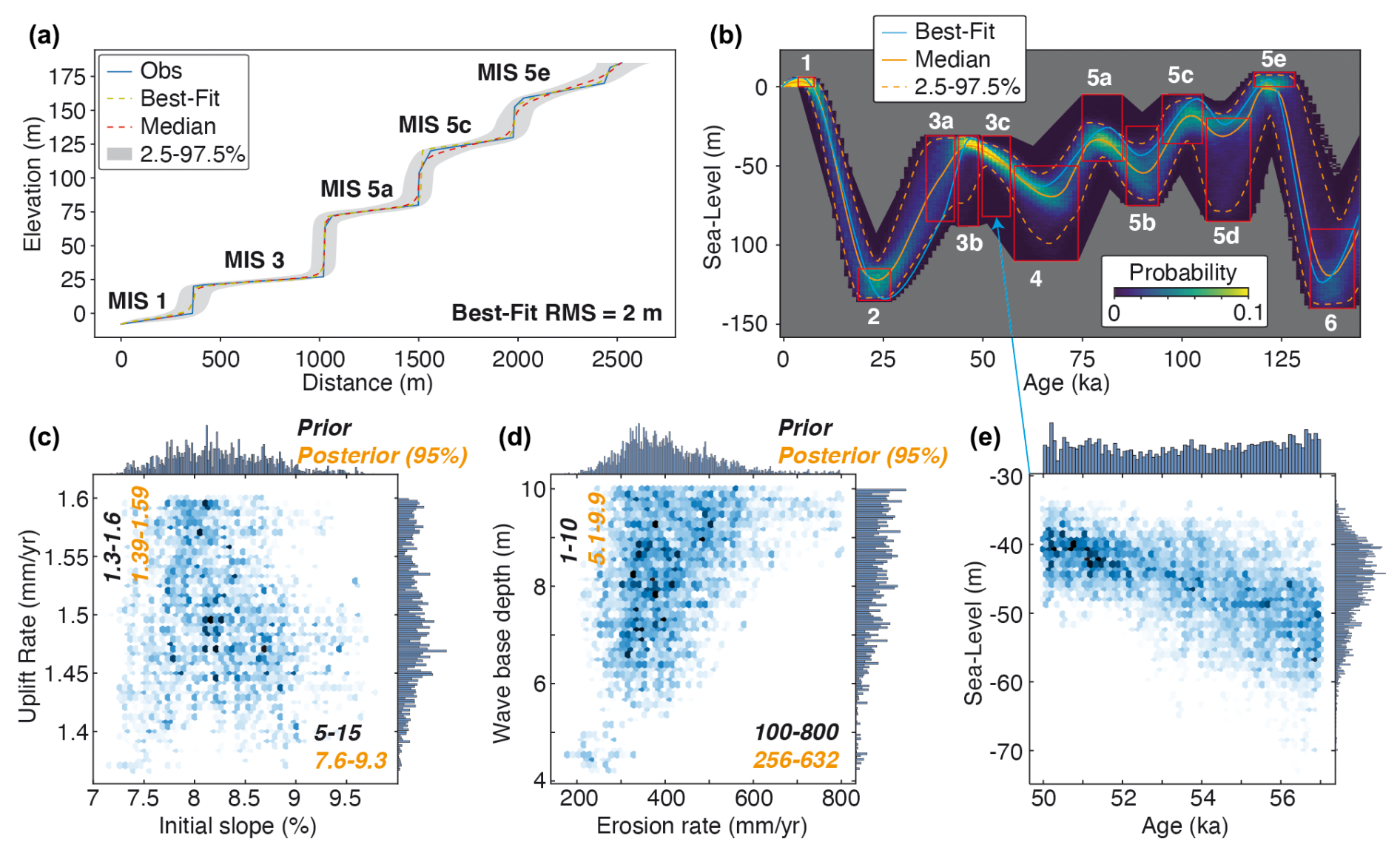
Figure 3 Inversion of NW Santa Cruz marine terrace sequence. (a) Observed topography (from Rosenbloom and Anderson, 1994; Obs, blue) with the age interpretation of Perg et al. (2001) marked in bold, together with the modeled best-fit, median, and 2.5 % and 97.5 % percentile profiles. (b) Probabilistic sea-level reconstruction for the profiles in (a), with MISs in white. (c) Posterior ranges for uplift rates and initial slopes (histogram of the sampled models). (d) Posterior ranges for wave-base depths and erosion rates. (e) Posterior ranges for the MIS 3c peak, i.e., distribution for the position of the 50–57 ka node within the paleo sea-level curve.

4 Santa Cruz marine terrace sequence inversion

The marine terraces along the Santa Cruz coastline (central California, US) formed through a combination of Quaternary sea-level oscillations and tectonic uplift by nearby active faults (e.g., Bradley, 1957; Anderson and Menking, 1994; Anderson et al., 1999; Perg et al., 2001; Matsumoto et al., 2022). We invert a topographic profile from Rosenbloom and Anderson (1994), who distinguished the original eroded bedrock surface, which we use, from its overlying colluvium for five marine terraces. We followed the age interpretation of Perg et al. (2001), suggesting these terraces were formed, from bottom to top, during MISs 1, 3, 5a, 5c, and 5e. Unlike in the synthetic tests, here we left uplift rate, erosion rate, wave-base depth, and initial slope parameters free within a prior range of values. We used the elevation (≈170 m) and age (≈118–128 ka) of the upper terrace to derive a range of possible uplift rates (1.3–1.65 mm yr⁻¹) and simultaneously consider ranges for initial slope (5 %–15 %), wave-base depth (1–10 m), and erosion rates (100–800 mm³ yr⁻¹) in the terrace inversion. We used the same inversion parameters as for the synthetic tests, running 1×10⁶ models over 450 ka, with the sea-level high- and lowstands limited to the red boxes in Fig. 1 (see the Supplement and Table S1). We tested different inversion parameters (Fig. S5), and settled on values of 1 m ipstep, 100 m σ, and 10 m corrl, as for these values the corresponding 95 % posterior ranges for the variability in terrace height (≈5 m; Fig. S5) and width (≈150 m; Fig. S5), are of the same order of magnitude as the variability in a swath profile across the Santa Cruz terraces (Fig. S6). Higher values for σ and corrl result in both broader ranges for accepted terrace heights/widths and, consequently, broader posterior ranges for paleo sea level, although we note that the first-order shape of the paleo sea-level curves remains similar, irrespective of the tested ipstep, σ, and corrl values (Fig. S5).

The sampled sea-level histories successfully reproduce the terrace morphology, as evidenced by the low misfit of 2 m (Fig. 3a). As with the synthetic tests (Fig. 2), periods of sea-level rise are better constrained than periods of sea-level fall and highstands are better constrained than lowstands (Fig. 3b). Also, here there is a trade-off in sea-level peaks, in which younger higher sea-level peaks could result in similar-shaped marine terraces to older lower sea-level peaks (e.g., for MIS 3c, Fig. 3e). The models limit the uplift rate to ≈1.35–1.6 mm yr⁻¹, the initial slope to ≈7 %–9.5 %, the wave-base depth to 4–10 m, and the erosion rate to 200–800 mm yr⁻¹ (Fig. 3c and d). Notably, there is a positive correlation between wave-base depth and erosion rate (Fig. 3d), suggesting that a higher value for wave-base depth would require a higher erosion rate to create the same marine terrace sequence morphology.

Compared with our proposed prior range of possible sea-level elevations for MIS 3 (−30 to −80 m; Fig. 3b), the posterior distribution of the inversion suggests paleo sea-level values on the higher end of that spectrum. This is in agreement with a growing number of studies suggesting that oxygen-isotope derived sea-level curves underestimate sea levels for that period (Pico et al., 2016; Dalton et al., 2019, 2022; Gowan et al., 2021; de Gelder et al., 2022). For MIS 5a, however, the posterior distribution of the inversion suggests a sea-level peak on the lower end of our proposed range of sea-level elevations (Fig. 3b). Although the highstand posterior distributions still span a broad elevation range of ≈25 m, these results tend to align with studies proposing an overall decrease in sea level between MISs 5e, 5c, and 5a (e.g., Chappell and Shackleton, 1986; Schellmann and Radtke, 2004; Tawil-Morsink et al., 2022).

We also tested additional uplift rate scenarios (Fig. S7), given that there have been concerns on the terrace chronology that we adopted (Brown and Bourlès, 2002) and other studies have suggested that the terrace at 27 m elevation might have been formed during MISs 5a, 5c, or 5e instead of MIS 3 (Bradley and Addicott, 1968; Lajoie et al., 1975; Kennedy et al., 1982; Weber et al., 1990). These uplift rates can fit the terrace sequence morphology equally well in terms of topographic misfit but generally imply a larger possible range of paleo sea levels. This can be explained by the increased terrace re-occupation for lower uplift rates (Malatesta et al., 2022), which also explains why the posterior ranges for the initial slope and wave-base depth change increase for lower uplift rate scenarios (Fig. S7) and erosion rate estimates decrease. These tests suggest that locations with higher uplift rates will generally provide narrower constraints on paleo sea levels, while still providing realistic and unbiased parameter estimates.

5 Gulf of Corinth marine terrace sequence inversion

The complexity of semi-isolated basins, connected to the sea during some time intervals and isolated in others, makes them ultimate testing grounds for our modeling approach. We focus on one such basin, the SE Gulf of Corinth, to derive a sea-/lake-level history from terrace sequence geometries and compare its outcomes with paleoclimate data, tectonic structures, and sill dynamics.

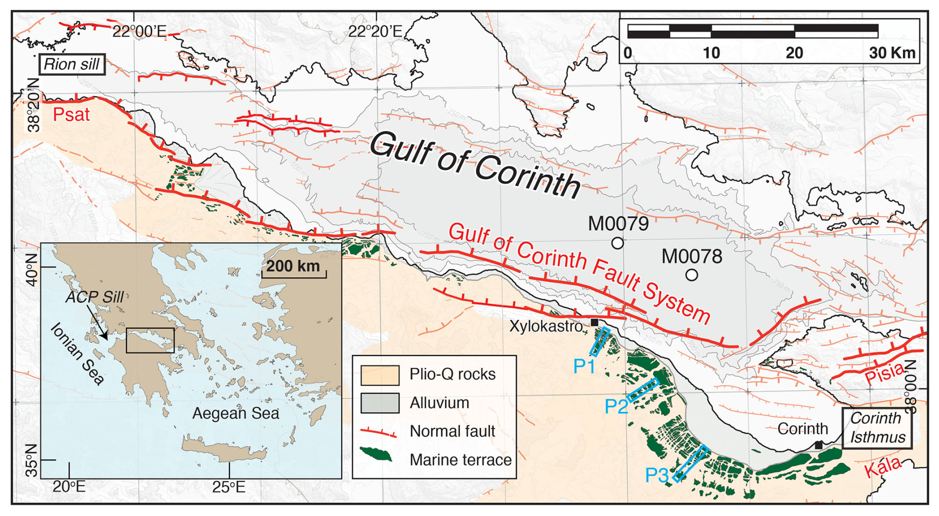
Figure 4 Tectonomorphology of the Gulf of Corinth. Main features of the Gulf of Corinth, including the active faults, marine terraces, and profile locations used in the inversion and connections to the Ionian Sea (Rion Sill) and Aegean Sea (Corinth Isthmus). M0078 and M0079 indicate the IODP-381 sedimentary coring locations (McNeill et al., 2019). Psat = Psathopyrgos Fault, Pisia = Pisia Fault, Kala = Kalamaki Fault. Modified from de Gelder et al. (2019) and Fernández-Blanco et al. (2019).

Natural interaction between the Gulf of Corinth and the open sea is currently restricted by the Rion and Acheloos-Cape Pappas sills at its W entrance at ≈45–60 m depth (Fig. 4; Beckers et al., 2016). In the past, there was an additional connection at its E end along the Corinth Isthmus, currently uplifted at ≈80 m elevation but consisting of Quaternary marine sediments (Fig. 4; Caterina et al., 2023). These sills have controlled the gulf's connection with the open sea over the past few hundred thousand years and have led to an alternation of marine and (semi-)isolated lake environments within the gulf (McNeill et al., 2019). Although we approximately know the timing of these alternations, it remains unclear whether sill depths remained stable or fluctuated throughout the Quaternary (Roberts et al., 2009; McNeill et al., 2019) and, in addition, whether lake levels were stable or fluctuating during periods with no connection to the sea. Hydroclimatic conditions, i.e., the balance between inflow, outflow, precipitation, and evaporation, determine the level of the lake; state-of-the-art paleo-environmental reconstructions (e.g., Kafetzidou et al., 2023) are insufficient to infer its fluctuations over time.

Terrace sequences are well exposed in the SE of the gulf, where the Gulf of Corinth fault system (Fig. 4) has led to differential coastal uplift rates (Armijo et al., 1996; de Gelder et al., 2019; Fig. S8). This peculiarity allows us to test, for a natural example, whether the joint inversion of multiple terrace sequence profiles with different uplift rates provides a better-constrained sea-/lake-level history (as in Fig. 2). To account for the unknown range of possible lake-level elevations, we carried out inversions with all nodes from (semi-)isolated periods broadly constrained between −15 and −150 m elevation. For the marine periods, we follow the more restricted eustatic sea-level ranges defined in Fig. 1b and c (red boxes), as the resulting posterior sea-/lake-level ranges would remain similar to the prior ranges for tests in which we also gave a lot of freedom to nodes for the marine periods (Fig. S4). We selected three topographic profiles with little river incision and ≈0.4–1.4 mm yr⁻¹ uplift rates (Fig. S8) and avoided modeling the broad coastal plains at the base of all profiles that appear to have been modified by human presence (Fig. S8). We used the 90 % percentile of 100 m wide swath profiles to obtain representative terrace sequence morphologies (Fig. S8). For the three profiles, we assigned prior ranges of possible uplift rates of 1.25–1.4, 0.7–0.9, and 0.4–0.55 mm yr⁻¹ (de Gelder et al., 2019; Fig. S8) and broad prior ranges for erosion rate (100–1500 mm yr⁻¹), initial slope (1 %–20 %), and wave-base depth (1–12 m).

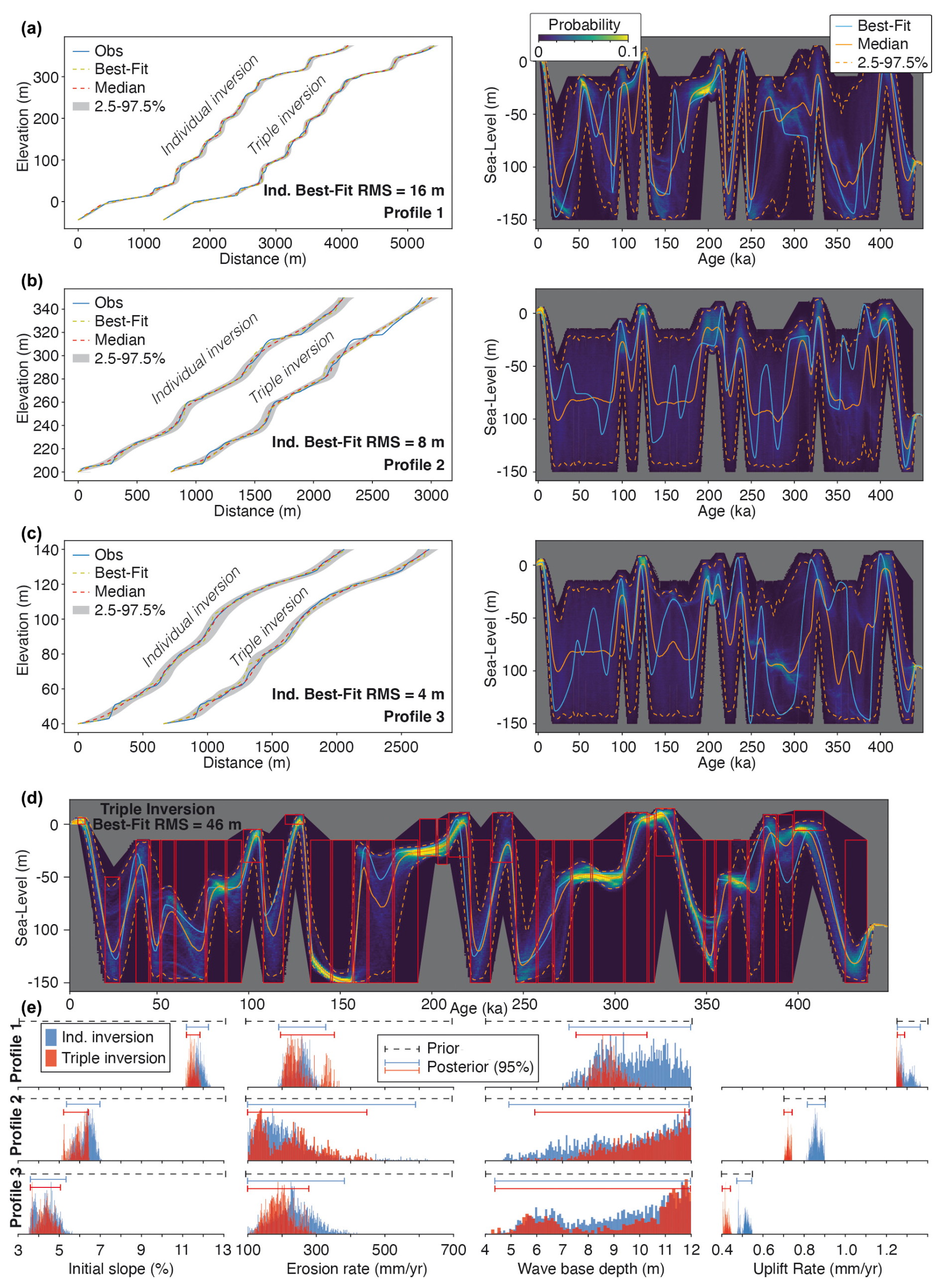
Figure 5 Inversion of SE Corinth Rift marine terrace sequence (see text). (a–c) Observed topography (left) from three different profiles in the SE Corinth Rift (for locations, see Fig. S8), together with the modeled best-fit, median, 2.5 %, and 97.5 % percentile profiles for both an individual profile inversion and a joint inversion of the three profiles (horizontally offset by an arbitrary value). Corresponding probabilistic sea/lake-level ranges for the individually inverted profiles are given on the right. (d) Posterior distribution for sea/lake-level history from joint inversion, with red boxes describing prior ranges. (e) Prior and posterior parameter ranges from both individual and joint profile inversions.

The individual profile inversions mostly constrain paleo sea/lake levels for profile 1 (Fig. 5a) because it has the highest uplift rate and contains the most terraces. The other two profiles provide limited constraints on paleo sea/lake levels when inverted individually (Fig. 5b and c) but when jointly inverted with profile 1 they provide a much narrower range in terms of posterior distribution for sea level (Fig. 5d). The cumulative misfit for the individual inversions (28 m) is slightly better than that for the joint inversion (46 m) but there are no major visible differences between the terrace sequence profiles for the two inversions and, apart from the highest terrace of profile 2 (Fig. 5b), the terrace sequences are all nearly perfectly reconstructed. The three profiles show variations in initial slopes that are in line with the overall morphology, i.e., present-day profile 1 is steeper than profile 2, which is steeper than profile 3, which is also what we find for their initial slopes. The three profiles do have similar posterior distributions for wave-base depths and erosion rates (Fig. 5e). Although we might expect lateral differences in these rates, given variability in sediment types, catchment area, and coastal orientation, the broad ranges for the posterior distributions indicate that we cannot quantify these lateral differences from the profile morphology alone. The posterior parameter ranges mostly remain the same between the individual and joint inversion, with the exception of the uplift rates for profiles 2 and 3, which become a little lower for the joint inversion. As for the sea-/lake-level inversion, all the other posterior parameter ranges become narrower for the joint inversion (Fig. 5e).

The inverted sea-/lake-level history (Fig. 5d) shows a few notable features. To a first order, fluctuations resemble global sea-level trends, with relatively fast periods of sea-/lake-level rise prior to major sea-level highstands, followed by long periods of slow sea-/lake-level fall (Fig. 1c). Yet, unlike global sea-level trends, there are several periods of prolonged stability, in particular around 180–200 and 275–300 ka and possibly also around 75–95 and 360–370 ka. In addition, glacial periods are often surprisingly poorly resolved, like during the period 20–75 or 160–180 ka. In the next section we discuss our interpretation of these trends and show how they provide insightful arguments to decipher the relation between water level, fault activity, paleoclimate, and tectonics.

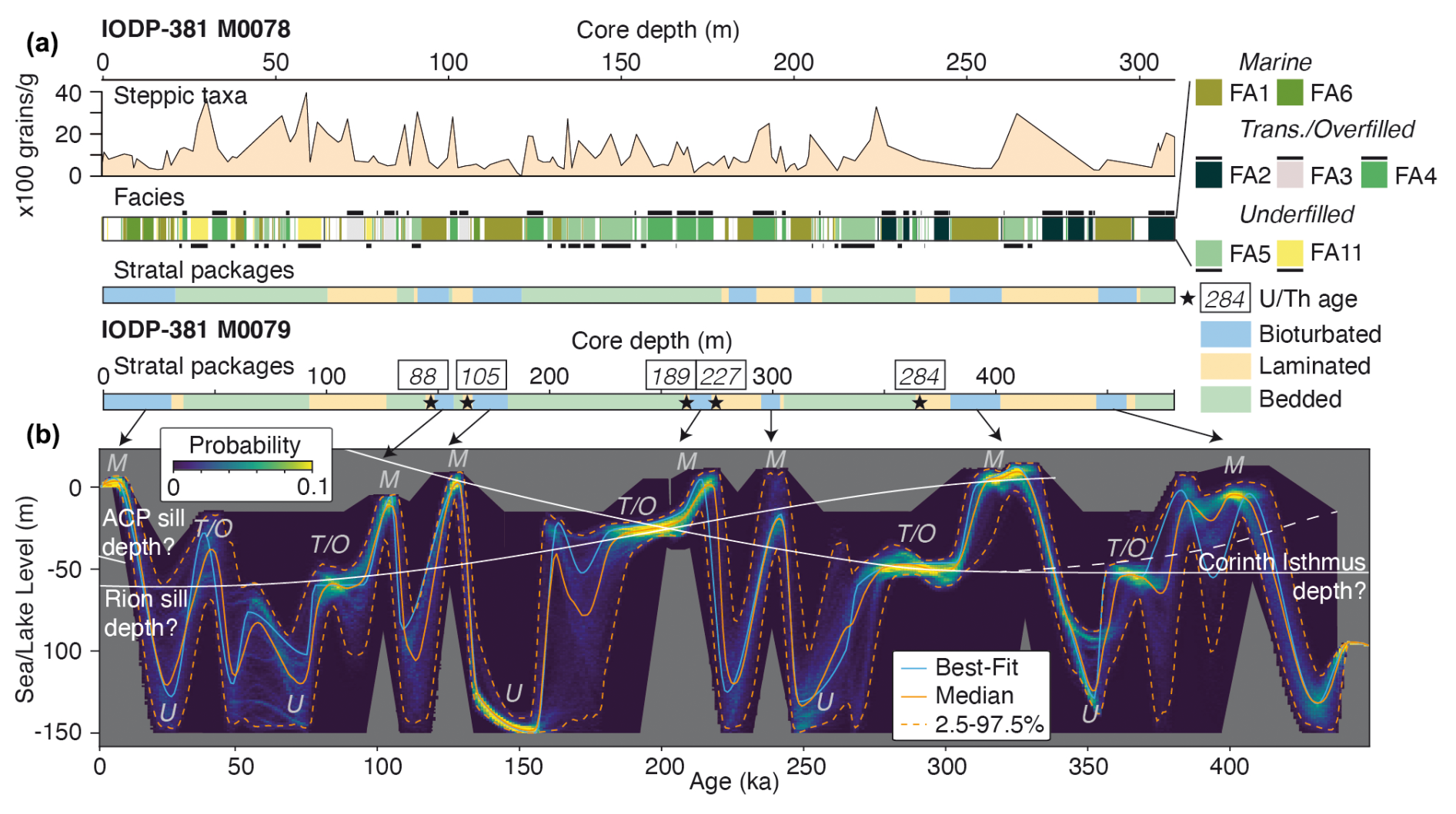
Figure 6 Comparison of sea-/lake-level reconstruction with other datasets. (a) Comparison with IODP-381 cores M0078 and M0079, with steppic taxa from Kafetzidou et al. (2023), facies from McNeill et al. (2019), and stratal packages with $\mathrm{U}/\mathrm{Th}$ ages from Gawthorpe et al. (2022). FA1 = homogeneous mud; FA2 = greenish gray mud with dark gray to black silty-to-sandy beds (centimeter scale); FA3 = light gray to white sub-millimeter laminations (calcite or aragonite) alternating with mud–silt beds; FA4 = laminated greenish gray to gray mud with muddy beds; FA5 = greenish gray mud with homogeneous centimeter-thick gray mud beds; FA6 = green bedded partly bioturbated mud, silt, and sand; FA11 = interbedded mud/silt and centimeter-thick sand beds. (b) Inversion result from Fig. 5d with proposed sill/isthmus elevations, marking periods with marine (M), transitional or overfilled (T/O), and underfilled (U) hydroclimatic modes.

6 Discussion

6.1 Beyond sea level: tectono-hydroclimatic processes in the Gulf of Corinth

While the results for the joint inversion of the three profiles in the Gulf of Corinth permit the unraveling of sea and lake levels through time, as expected, we also stress that such inversions yield more, when integrated within the broader environmental setting: these reconstructions allow for a more detailed look into sea- and lake-level fluctuations within a (semi-)isolated basin. Figure 6 compares our inverted sea-lake level with the stratigraphy, facies, and pollen content within two sedimentary cores from the sea floor of the central basin (McNeill et al., 2019; Gawthorpe et al., 2022; Kafetzidou et al., 2023). Based on those combined datasets, we propose that the main hydroclimatic modes that have occurred in the Gulf of Corinth throughout the past 450 ka are (1) marine Gulf of Corinth, (2) transitional Gulf of Corinth or overfilled Lake Corinth, and (3) underfilled Lake Corinth. The first two of those have been proposed before, based on sedimentary cores (McNeill et al., 2019; Gawthorpe et al., 2022), whereas we base the occurrence of intervals with an underfilled Lake Corinth on our marine/lake terrace inversion, as available paleoclimatic proxies are unable to uncover them.

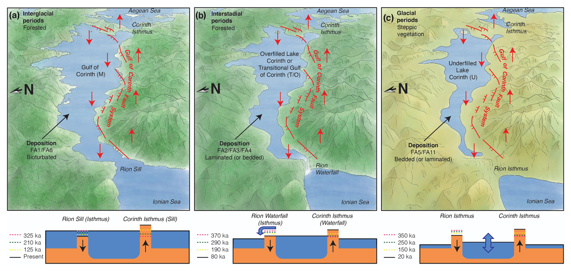
Figure 7 Different hydroclimatic modes in the Lake/Gulf of Corinth. (a) The interglacial marine (M) hydroclimatic mode as it is today. Around MIS 5e (≈125 ka), the marine connection also occurred above the Rion Sill, with the Corinth Isthmus a land bridge like it is today. Around MISs 7a–e (≈210–240 ka) and MIS 9 (≈325 ka), the marine connection occurred above both the Rion and Corinth sills. Around MIS 11 (≈400 ka), the marine connection would have occurred above the Corinth Sill, with the Rion Isthmus on the W end of the Gulf of Corinth. (b) The transitional or overfilled (T/O) hydroclimatic mode at ≈80 ka, with a narrow connection or waterfall to the open sea at the Rion Sill. Around ≈190 ka, a narrow connection or waterfall to the open sea could have occurred at either or both of the Rion and Corinth sills and at ≈290 and ≈370 ka only at the Corinth Sill, with the Rion Isthmus on the W end of the Gulf of Corinth. (c) The underfilled (U) hydroclimatic mode at ≈20 ka. As for the older glacial periods (≈150, ≈250, and ≈350 ka), land bridges occur on both side of Lake Corinth, at the Rion and Corinth isthmuses. In all illustrations, red arrows indicate uplift and subsidence in the footwall and hanging wall of the Gulf of Corinth fault system, respectively.

The major peaks in our reconstructed sea/lake-level curve occurred during interglacial sea-level highstands, as a direct consequence of our choices in the ranges of the priors, when the sea level in the Gulf of Corinth was similar to the eustatic sea level (marine mode M; Fig. 7a): sedimentary cores indicate marine conditions (McNeill et al., 2019), the corresponding stratal packages are bioturbated, and associated sedimentary facies are types FA1 and FA6 (Fig. 6; see caption for facies description). From pollen records, the typical reconstructed biomes are cool mixed evergreen needleleaf and deciduous broadleaf forests, indicating relatively warm and wet conditions with low amounts of steppic taxa (Kafetzidou et al., 2023; Fig. 6).

We interpret the interstadial periods around 75–95, 180–200, 275–300, and 360–370 ka as periods with an overfilled Lake Corinth, possibly with some marine incursions indicating a transitional Gulf of Corinth (T/O mode; Fig. 7b). This would explain the prolonged sea-/lake-level stability during interstadial periods, when the eustatic sea level fluctuated by tens of meters (e.g., Spratt and Lisiecki, 2016; de Gelder et al., 2022). In that case, sea-/lake-level elevations would correspond to the paleo-sill depth of the Rion Sill and/or the Corinth Isthmus (white line, Fig. 6). Within the sedimentary cores, these periods are mostly characterized by laminated stratal packages; associated sedimentary facies are types FA2, FA3, and FA4 (Fig. 6; see caption for facies description). The occurrence of marine incursions into Lake Corinth during these interstadial periods is suggested by dated corals of ≈76, ≈178, and ≈201 ka (Roberts et al., 2009; Houghton et al., 2003), as well as the white aragonite-rich laminations of FA3 and FA4. In other locations, such laminations have been linked to (seasonal) mixing of marine and nonmarine surface waters (Sondi and Juračić, 2010; Roeser et al., 2016).

The glacial periods are characterized by relatively low sea/lake-level elevations, possibly even down to the lower limit of −150 m we used in the inversion. We interpret these periods as underfilled Lake Corinth conditions (U mode; Fig. 7c), during which water inflow was lower than water evaporation within the lake and lake level fell down to tens of meters below the sill depth. Sedimentary cores indicate nonmarine conditions (McNeill et al., 2019); the corresponding stratal packages are mostly bedded and associated sedimentary facies are types FA5 and FA11 (Fig. 6; see caption for facies description). Reconstructed biomes from pollen suggest an increase in open vegetation, such as grassland and steppe, communities under colder and drier conditions (Kafetzidou et al., 2023; Fig. 6), matching reconstructed periods of lake underfilling. In general, the inverted resolution of the lake-level elevation is much lower for these periods, with large probabilistic ranges. We attribute this to the occurrence of rapid lake-level fluctuations, like in other isolated east Mediterranean water bodies, such as the Dead Sea (Stein et al., 2010) and Lake Van (Türkiye; Landmann et al., 1996). In such environments, the lake level is determined by the budget between runoff and evaporation, and quick variations are expected. Alternatively, this could also be due to the fact that terraces formed during low sea/lake level get increasingly eroded during transgressions.

The interstadial periods with prolonged sea-/lake-level stability also allow for a possible reconstruction of sill depths through time (white lines, Fig. 6). The westernmost sill, the Acheloos-Cape Pappas Sill (Fig. 4), is currently at a depth of ≈45–48 m. While there are no major faults there, we cannot exclude slow subsidence or uplift at a few tenths of millimeters per year, cumulating to a few tens of meters on the 100 kyr timescale. The Rion Sill, at the western entrance to the Gulf of Corinth, is currently at ≈62 m depth (Perissoratis et al., 2000). As it is located in the hanging wall of the Psathopyrgos Fault (Fig. 4), active since at least the past ≈200 ka (Houghton et al., 2003), the Rion Sill was unlikely to have been deeper in the past. We reconstruct the Rion Sill depth, assuming that marine incursions around ≈76 ka (Roberts et al., 2009) took place through this sill and that the Rion Sill was not lower than the sea/lake level during the overfilled/transitional interval around ≈200 ka. Extrapolating the trend, it would make sense for the older connections between the Lake/Gulf of Corinth and the open sea to have occurred primarily through the Corinth Isthmus at the eastern end of the Gulf of Corinth.

The Corinth Isthmus is currently at an elevation of ≈80 m and has been uplifted through the Pisia Fault, the Kalamaki Fault, and/or a regional uplift (Armijo et al., 1996; Roberts et al., 2009; Caterina et al., 2023). We reconstruct the Corinth Isthmus depth, assuming that lake/sea levels during overfilled/transitional intervals around ≈290 and ≈360 ka correspond to the Corinth Isthmus depth and that the isthmus was not lower than the sea/lake level during the overfilled/transitional interval around ≈200 ka. Extrapolating this trend fits with the current Corinth Isthmus elevation of ≈80 m. The isthmus elevation before ≈360 ka is difficult to constrain from our data but was possibly shallower before, given the small amount of marine sediments deposited around the ≈400 ka interglacial period and the lack of deposits within the isthmus stratigraphy older than ≈350 ka (Collier and Dart, 1991; Caterina et al., 2023). Our reconstruction of both the Rion Sill and the Corinth Isthmus fits with the sedimentary interpretation of a tidal strait around ≈300 ka at the isthmus, with marine connections on both ends of the Gulf of Corinth (Caterina et al., 2023).

Our exploration of sea-/lake-level variations in the Gulf of Corinth demonstrates the strength of using marine/lacustrine terrace sequence inversion. Although several questions remain – like the effects of erosion and sedimentation on sill evolution or the effects of nonconstant uplift rates of the marine terrace sequences – we are able to provide a solid framework that can explain several different tectonic and hydroclimatic processes simultaneously. Furthermore, our results may provide a window to explore the links between paleogeographic and biologic evolution, with our proposed history of sills, waterfalls, and land bridges (Fig. 7) theoretically impacting temporal isolation and mixing of species between the Peloponnese and the Greek mainland. We distinguish four different hydroclimatic modes for the Lake/Gulf of Corinth that have probably also occurred in other (semi-)isolated basins, like the Sea of Marmara or the Cariaco Basin. Marine and transitional modes will most likely depend on eustatic sea-level elevations and sill depths, whereas over- or underfilled lakes probably depend on sill depths and local climatic conditions. For Corinth Lake, we show that this transition from over- to underfilled lakes occurs during changes from interstadial to glacial periods, and is accompanied by changes in vegetation that imply drier conditions.

6.2 Inversion of marine terrace sequences

In these examples, we showed how to assess paleo sea-level variations and simultaneously extract quantified metrics for morphotectonics and hydrodynamics from the geometry of marine terrace sequences. Using a probabilistic inversion methodology set in a Bayesian framework, we avoid the simplifications of bijective approaches in which a single marine terrace is always linked to a single sea-level highstand and vice versa (e.g., Pastier et al., 2019; Malatesta et al., 2022). By considering a full sea-level curve and its possible variability, it is possible to provide quantitative constraints on highstands, lowstands, and sea-level rise and fall, filling the observational gap for time periods for which field measurements are scarce. We admit that some model simplifications and approximations may alter our interpretations. In particular, we neglected subaerial erosion and kept uplift rate, erosion rate, initial slope, and wave-base depth parameters time-constant for each individual sampled paleo sea-level curve. Both could be fine-tuned in future developments.

To apply this model procedure to other sites, we can make several recommendations based on our findings in this study. Any coastal area with marine terraces will have a lateral variability in terms of terrace width and terrace elevation. Given that the posterior ranges for the model parameters (paleo sea level, uplift rate, etc.) will directly depend on the chosen inversion parameters (ipstep, σ, and corrl), it is important to adjust those inversion parameters to the naturally observed variability in the geometry of a marine terrace sequence. In the Santa Cruz example, the similarity in terrace width/height variability between the modeled posterior ranges (Fig. S5), and the observed variability within a section of the marine terrace sequence (Fig. S6), justifies our choice of inversion parameters. But if we wanted to characterize a larger area along the Santa Cruz coastline, we would have to increase σ and/or corrl to account for the higher degree of variability or jointly invert multiple cross-sections in which every cross-section has a similar variability in terrace height/width.

The prior information required to obtain reliable results will also be dependent on the context of a specific marine terrace sequence and on the parameter cut-off choices deemed realistic. For Santa Cruz and Corinth, the posterior distributions for wave-base depth suggest that, purely based on marine terrace sequence morphology, this cut-off could have been deeper than 10–12 m (Figs. 3 and 5). However, based on observations and models of cliff erosion, it seems unlikely that the wave base for bedrock erosion is more than 10 m for Santa Cruz (Kline et al., 2014); wave-base depths/heights should be smaller for the calmer Gulf of Corinth. This choice of cut-off in turn affects the posterior distribution of other parameters and should thus be chosen carefully.

In the cases of Corinth and Santa Cruz, we assigned relatively narrow windows for the uplift rate, based on chronological information that was already available. As such, we only obtained refinements, rather than “new” information about the uplift rate. For the Santa Cruz case, we tested four uplift rate scenarios matching different possible chrono-stratigraphies (Fig. S7) that could all explain the morphology equally well, albeit with different ranges for the other parameters. We also inverted the Santa Cruz terrace sequence morphology with a broad range between 0.3 and 1.5 mm yr⁻¹ but the inversion would converge on only one of the four scenarios in Fig. S7. This suggests that at least an approximate prior idea of the uplift rate is a prerequisite for a reliable inversion of a marine terrace sequence morphology.

Many paleo sea-level studies that use geomorphic/geologic observations tend to have a confirmation bias regarding sea-level curves and propose refinements of paleo sea-level estimates to sub-meter scale (e.g., Murray-Wallace, 2002; Roberts et al., 2012) or uplift rates to precisions of ∼0.01 mm yr⁻¹ (e.g., Pedoja et al., 2018; Meschis et al., 2022). In this study, we take a step back by allowing more freedom to vary possible paleo sea-levels, as well as uplift rate, erosion rate, initial slope, and wave-base depth, to provide a more reliable way to translate morphologic observations to paleo sea-level constraints. For instance, the low uplift rate examples from the Corinth Rift (Fig. 5b and c) and Santa Cruz (Fig. S7) reveal very little about paleo sea/lake levels, even if the uplift rate is roughly known. As a marine terrace is formed over several sea-level cycles, the resulting terrace width and height will depend on all those cycles, as well as wave-base depths, erosion rates, and initial slopes, all of which are generally poorly constrained. Even in the hypothetical case that these parameters are known (Fig. 2), there is still a wide spectrum of sea-level histories that could have created the specific morphology of a marine terrace sequence. This suggests that estimating paleo sea levels based on the comparison of a present-day landform with a paleo-landform (Rovere et al., 2016) may be too simplistic in many cases, at least for erosive marine terraces. Although the uncertainties that we provide on paleo sea levels are much larger than calculations based on hydrodynamic ranges would suggest (Lorscheid and Rovere, 2019), we do consider them to be reliable as they take in a large number of unknowns. To reduce uncertainties, we demonstrated in this paper that a joint inversion of multiple profiles is a powerful way forward.

For simplicity, as the aim of this paper was to test the model on increasingly complex settings, we only inverted one profile for Santa Cruz and three for Corinth but it is easily possible for explorations to use more profiles at those locations in future work. In addition, although here we focused on erosive marine terraces to develop a proof of concept, another promising avenue is to apply this inversion method to bio-constructed (coral reef) terraces, which tend to be better dated (e.g., Pedoja et al., 2014; Hibbert et al., 2016), and for which modeling routines also exist (e.g., Toomey et al., 2013; Pastier et al., 2019). One of our key findings is that inverting multiple profiles simultaneously provides much better paleo sea-level constraints than focusing on individual profiles (Figs. 2 and 5). The global archive of paleo-shorelines (Fig. 1a) presents a huge potential for such multi-profile marine terrace inversions. Not only would this massive inversion lead to improved estimates of local relative sea-level histories but it may also complement studies on glacio-isostatic adjustments that are relevant to a global sea-level perspective.

7 Conclusions

In this study, we demonstrated the use of a probabilistic inversion approach to decipher the formation of marine terrace sequences, in general, and the tectonic and hydroclimatic evolution of (semi-)isolated basins, in particular. With this approach, we provide the tools (see below) to simultaneously estimate past sea-level variations, uplift rates, erosion rates, initial slopes, and wave heights.

From synthetic tests, benchmarking on a terrace sequence near Santa Cruz marine terrace sequence, and application to the sequence in the SE Gulf of Corinth, our results bring a theoretical advance by showing the following. (1) Paleo sea level and other parameter ranges can be better constrained from sequences that are uplifting at higher rates, compared with lower rates, and better constrained from a joint inversion of multiple profiles than from inversion of a single profile. (2) Uplift rates, sea-level variations, and wave erosion parameters are intricately linked. By allowing more freedom to possible ranges of all the relevant parameters, we provide a more reliable way to translate morphologic observations to paleo sea-level constraints. Resulting uncertainties may be higher, compared with “classic” approaches of comparing present with past shoreline elevations, but are more realistic. (3) Probabilistic inversion of marine terrace sequences is a powerful method, applicable to a large portion of the world's coastlines, to disentangle tectonic and hydroclimatic processes.

Beyond the methodological achievement, by applying our method to a complex case – the semi-isolated Gulf of Corinth (Greece) – we show that this method can be a powerful tool to explore subtle environmental forcings, like the balance between precipitation and evaporation, that may have had a prime importance in setting the lake level during certain periods of time. We found that the eustatic sea level and tectonically changing sill depths drive marine and transitional phases during interglacial and interstadial periods, respectively. Wetter and drier conditions drive over- and underfilling of Lake Corinth during interstadial and glacial periods, respectively. We expect such transitions to be different for each unique tectono-hydroclimatic setting, with our inversion approach providing a new way to decipher such geomorphic Rosetta stones.