the Creative Commons Attribution 4.0 License.
the Creative Commons Attribution 4.0 License.
 | 19 Dec 2022
A combined approach of experimental and numerical modeling for 3D hydraulic features of a step-pool unit
Chendi Zhang
Yuncheng Xu
Marwan A. Hassan
Mengzhen Xu
Pukang He
Step-pool systems are common bedforms in mountain streams and have been utilized in river restoration projects around the world. Step-pool units exhibit highly nonuniform hydraulic characteristics which have been reported to closely interact with the morphological evolution and stability of step-pool features. However, detailed information on the three-dimensional hydraulics for step-pool morphology has been scarce due to the difficulty of measurement. To fill in this knowledge gap, we established a combined approach based on the technologies of structure from motion (SfM) and computational fluid dynamics (CFD). 3D reconstructions of bed surfaces with an artificial step-pool unit built from natural stones at six flow rates were imported to CFD simulations. The combined approach succeeded in visualizing the high-resolution 3D flow structures for the step-pool unit. The results illustrate the segmentation of flow velocity downstream of the step, i.e., the integral recirculation cell at the water surface, streamwise vortices formed at the step toe, and high-speed flow in between. The highly nonuniform distribution of turbulence energy in the pool has been revealed, and two energy dissipaters of comparable magnitude are found to co-exist in the pool. Pool scour development during flow increase leads to the expansion of recirculation cells in the pool, but this expansion stops for the cell near the water surface when flow approaches the critical value for step-pool failure. The micro-bedforms (grain clusters) developed on the negative slope affect the local hydraulics significantly, but this influence is suppressed at the pool bottom. The drag forces on the step stones increase with discharge (before the highest flow value is reached). In comparison, the lift force consistently has a larger magnitude and a more widely varying range. Our results highlight the feasibility and great potential of the approach combining physical and numerical modeling in investigating the complex flow characteristics of step-pool morphology.
- Article
(13755 KB) - Full-text XML
-
Supplement
(3161 KB) - BibTeX
- EndNote


Step-pool morphology is commonly formed in high-gradient headwater streams (Montgomery, and Buffington, 1997; Lenzi, 2001; Church and Zimmermann, 2007; Zimmermann et al., 2020). This bed structure has been reported to contribute to providing diverse habitats for aquatic organisms (Wang et al., 2009; O'Dowd and Chin, 2016), efficiently dissipating flow energy (Wilcox et al., 2011; Zhang et al., 2020) and enhancing channel stability (Lenzi, 2002; Wang et al., 2012). Artificial step-pool systems mainly composed of boulders mimicking natural channel morphology have been applied in restoration projects in steep channels with the objective of improving local ecology and riverbed stability (e.g., Wang et al., 2012; Smith et al., 2020). To facilitate the application of artificial step-pool systems, an advanced understanding of the morphology, hydraulics, and stability of step-pool features, as well as the interaction between them is needed. High-resolution information on both topography and hydraulics for step-pool features is fundamental for understanding such interactions.
Recently, advanced information on the morphological evolution of step-pool features has been obtained by the rapidly developing technology of structure from motion with multi-view stereo (SfM-MVS, together referred to as SfM in this paper) photogrammetry (e.g., Zhang et al., 2018, 2020; Smith et al., 2020). SfM photogrammetry provides topographic reconstructions with high spatial resolution and precision using easily accessible consumer-grade cameras or unmanned aerial vehicle (UAV) systems (Eltner et al., 2016; Morgan et al., 2017; Tmušić et al., 2020; Zhang et al., 2022). Although detailed topographic information has been made available through SfM photogrammetry, access to high-resolution hydraulic information remains limited for step-pool features. This incompatibility in the spatial resolution between morphological and hydraulic data hinders advancements in understanding how these two aspects interact with each other.
Unlike topography, detailed measurements of the 3D flow properties of a step-pool unit are rarely accessible due to the highly nonuniform, aerated, and turbulent flow regimes resulting from the alternation between supercritical (jet) and subcritical (jump) flow conditions (Church and Zimmermann, 2007; Wang et al., 2012; Zimmermann et al., 2020). Also, the formative flows of step-pool morphology are exceptional floods with a return period of about 50 years (Lenzi, 2001; Turowski et al., 2009), making hydraulic measurement impractical in the field. Tracer-based techniques (e.g., Waldon et al., 2004; Zimmermann et al., 2010) were used to characterize reach-scale flow properties in step-pool morphology; however, these can hardly reflect the nonuniform features of hydraulics along the sequence. Point measurements for flow velocity around step-pool features could be achieved by using an acoustic Doppler velocimeter (Wilcox et al., 2011; Li et al., 2014) or electromagnetic current meter (Wohl and Thompson, 2000; Wilcox et al., 2011). Such measurements have the merit of high temporal resolution but with limited spatial resolution as the arrangement of measured points is significantly affected by the rough beds and shallow water depths in mountain streams (Wilcox et al., 2011). These techniques are also more suitably used at low to moderate flows rather than at high flows during which significant sediment transport may occur and threaten the safety of such equipment. Particle tracking velocimetry (PTV, Maas et al., 1993) and particle image velocimetry (PIV, Adrian, 2005) techniques have been applied to measure the flow field for step-pool units in flume experiments (Zhang et al., 2018, 2020). The recirculation at the step toe and the high-speed flow impinging at the pool bottom were visualized by the PTV method near flume side walls, while the strong contrast of surface flow velocities at the step and pool areas has been illustrated based on the PIV method. However, these measurements were limited to the side walls and water surface. Another problem was that the highly nonuniform flow characteristics led to uneven distribution of tracer particles over step-pool units, leading to significantly reduced accuracy in areas with a low density of tracer particles (e.g., Zhang et al., 2020).
Nevertheless, the challenges of directly measuring the nonuniform hydraulic features of a step-pool unit present opportunities for 3D computational fluid dynamics (CFD) modeling. CFD simulations have been applied in research addressing flow dynamics with highly turbulent free surfaces generated by complex structures in the channel (e.g., Thappeta et al., 2017; Xu and Liu, 2016, 2017; Lai et al., 2021; Zeng et al., 2021) or irregular boundaries of the channel (e.g., Chen et al., 2018, 2022; Roth et al., 2020). This numerical approach has shown great promise in characterizing and visualizing complex 3D hydraulic features at high spatial and temporal resolutions. Furthermore, the flow forces on structures or topography which directly drive the interaction between hydraulics and morphology can also be captured by CFD modeling (e.g., Xu and Liu, 2016; Chen et al., 2019).
The CFD approach has been applied in studies containing step-pool features which were conceptualized by highly simplified 2D geometry mimicking the stepped spillway with flat surfaces (e.g., Thappeta et al., 2021). Although this simplification reflects some unit-scale geometric properties of step-pool features (e.g., step length and height), it fails to characterize the subunit-scale morphological features such as the transverse variability in the topography of step crests (Wilcox et al., 2011), the shape of the scour hole (Comiti et al., 2005), and the grain clusters developed in the pool (Zhang et al., 2020). Furthermore, to our knowledge flow forces on step-pool units have not been simulated in CFD models and have only been analyzed theoretically (Weichert, 2005; Zhang et al., 2016). Therefore, we see great potential for CFD simulations using configurations that reconstruct natural step-pool morphology by the SfM method in capturing the high-resolution hydraulic properties and flow forces of step-pool features.
The objective of this study is to acquire the high-resolution three-dimensional hydraulics for a step-pool unit built with natural stones and then examine the 3D distribution of flow velocity, turbulence, coherent structures, and flow forces on the bed surface. To address our objectives, we established a combined approach of physical and numerical modeling of the 3D hydraulics of a step-pool unit and analyzed the 3D distribution of flow properties and forces. The three-dimensionality of flow characteristics, mechanisms of energy dissipation, and interaction between hydraulics and morphological evolution for a step-pool unit are discussed, while insights into the stability and failure of step-pool units are also provided. Finally, the limitations of the combined approach are summarized.
The general workflow for the combined approach is presented in Fig. 1. The 3D topographic models of a step-pool unit were obtained by SfM photogrammetry in the flume experiment of Zhang et al. (2020) and were used as inputs for the CFD simulations, which were verified with the measurements of the water surfaces. Details of the flume measurements and CFD simulations are presented in Sects. 2.1 and 2.2, respectively, followed by the model verification in Sect. 2.3 and the processing methods for the model outputs in Sect. 2.4.
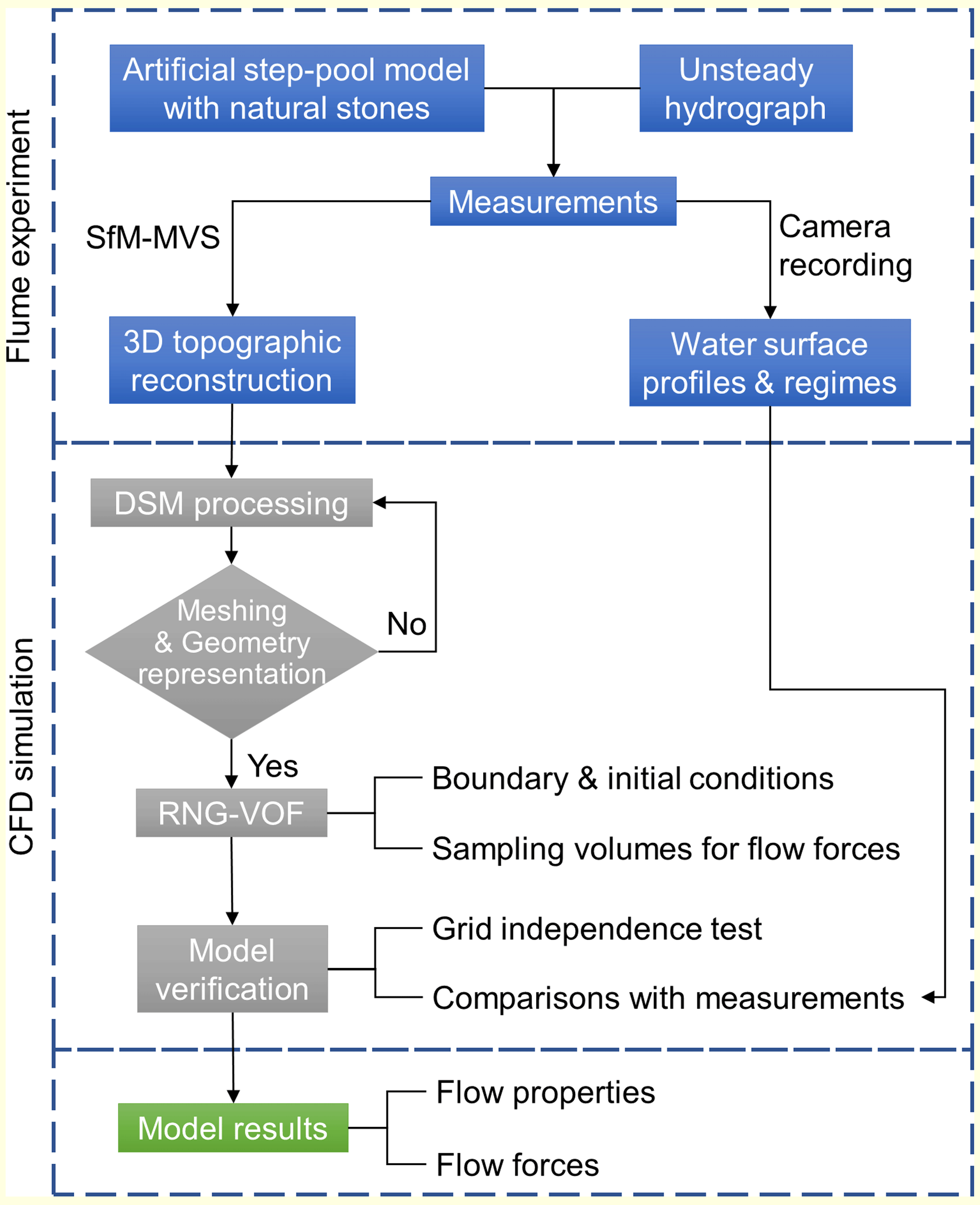
Figure 1Workflow of the combined approach. SfM-MVS refers to the technology of structure from motion with multi-view stereo. DSM is short for digital surface model. RNG-VOF is short for renormalized group (RNG) k−ε turbulence model coupled with the volume of fluid method.
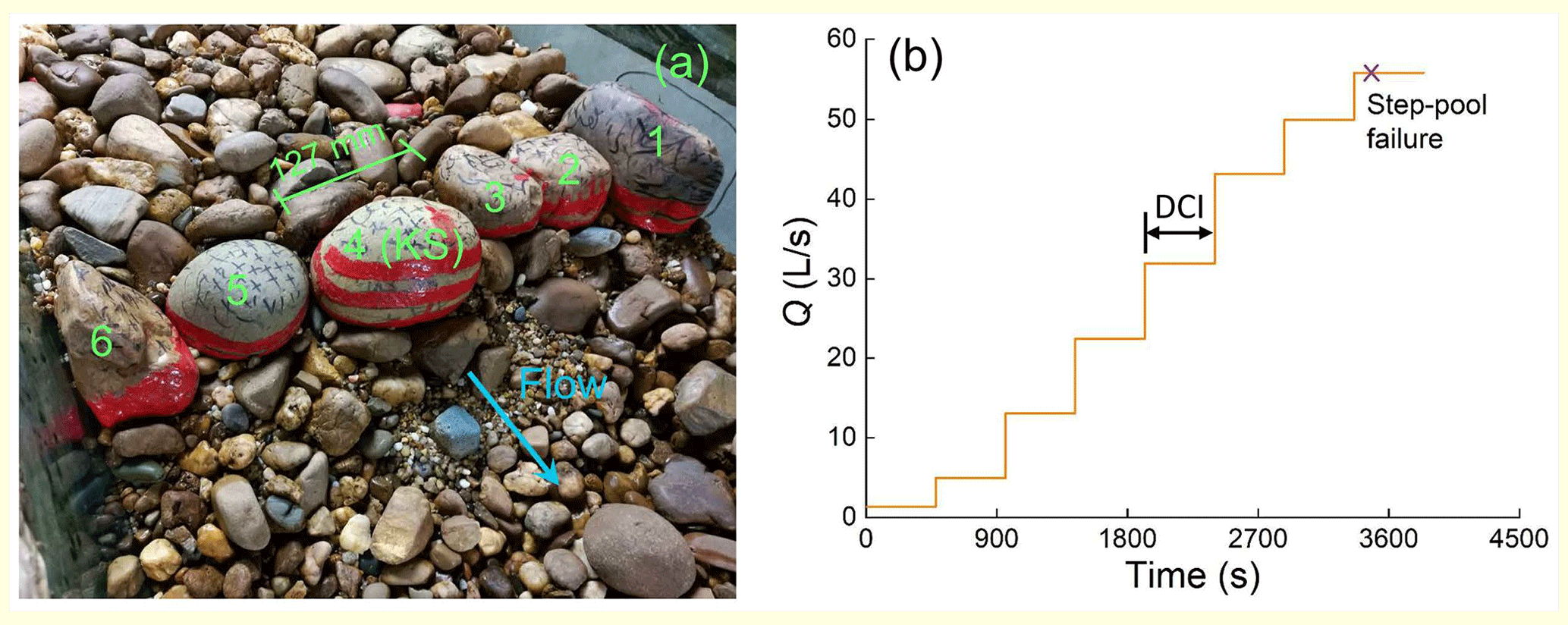
Figure 2Flume experiment settings in Zhang et al. (2020): (a) the artificially built-up step-pool model using natural stones with stone number labeled and (b) the unsteady hydrograph of the run used in this study. KS in (a) is short for keystone, and DCI in (b) is discharge change interval. The run index in (b) is CIFR (continually increasing flow rate) T2.
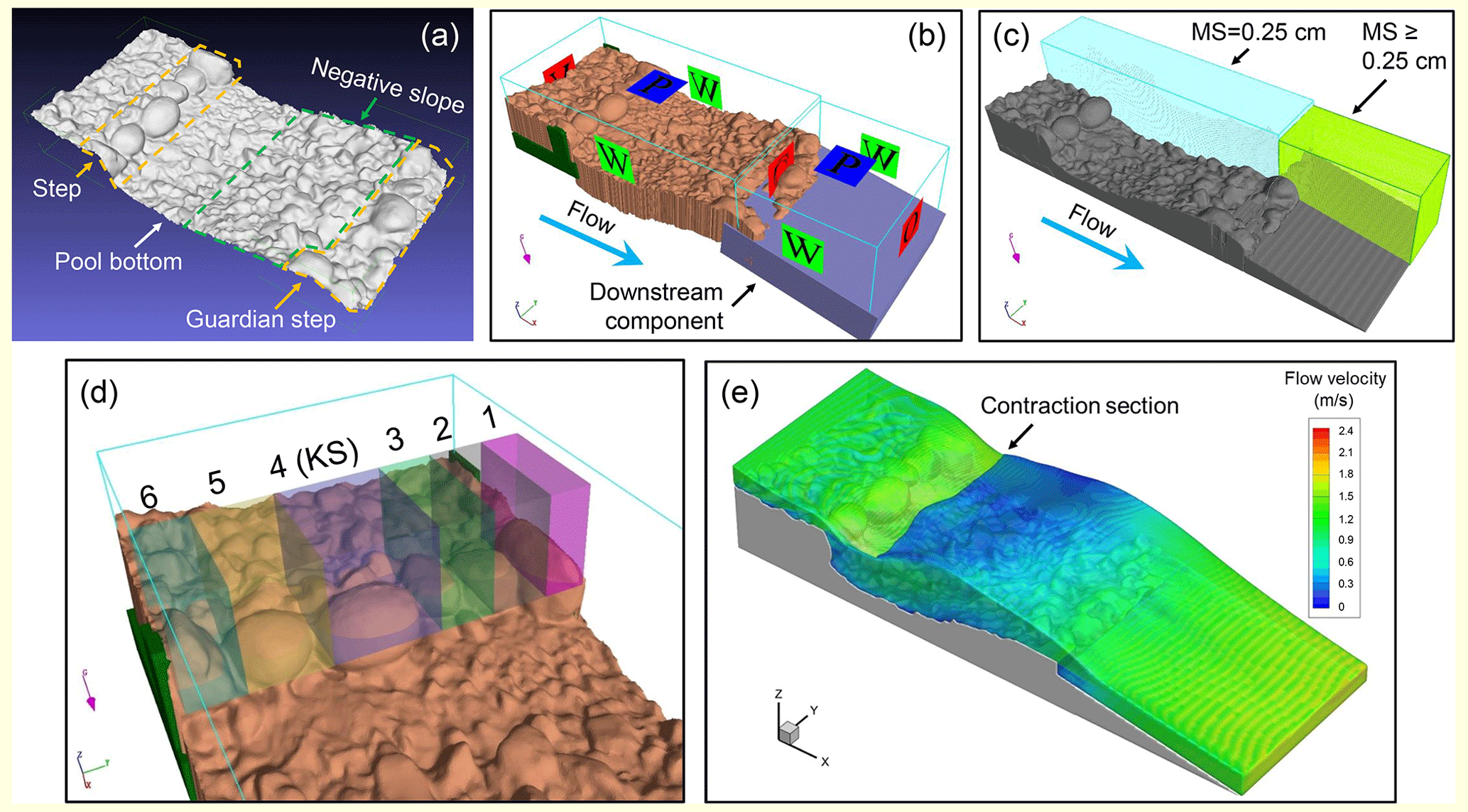
Figure 3Setup of the CFD model. (a) Three-dimensional digital surface model (DSM) of the step-pool unit by the SfM-MVS method as the input to the 3D CFD modeling. (b) Extruded bed surface model connected to the extra downstream component (in purple blue) and rectangular columns to fill leaks (in green), with the boundary conditions shown on mesh planes. (c) Recognized geometry in FLOW-3D with two mesh blocks (the upstream block had uniform mesh size, while the downstream one had nonuniform mesh size); MS is short for mesh size. (d) Sampling volumes to capture the flow forces acting on each step stone at X, Y, and Z directions. (e) An example for the simulated 3D flow over the step-pool unit colored by velocity magnitude at the discharge of 49.9 L s−1. The abbreviations for boundary conditions in (b) are V for specified velocity, C for continuative, P for specific pressure, and W for wall condition. The contraction section in (e) refers to the cross-section where the jump component starts in the pool.
2.1 Flume experiment
Since details of the flume system and experimental settings have been reported in Zhang et al., (2018, 2020), only a brief description of the experimental setup is presented here. The glass–steel-walled flume was 0.5 m wide and 0.6 m deep with a working length of 7.0 m. The initial slope of the sediment mixture was set at 3.2 %. A top-mounted camera (1920 × 1080 px2, with a maximum frequency of 60 fps) was installed above the flume to capture images of the surface flow features. Two side cameras were used to capture the longitudinal profiles of the bed and water surface near the flume walls (see details in Sect. S1 in the Supplement). A step-pool model was manually constructed by arranging six natural stones (Fig. 2a) with a b axis of 76–104 mm. The D50 (the grain size at which 50 % of the material by weight is finer) of the entire sediment mix in the flume was 20 mm (Zhang et al., 2018), with Dmax and D84 of 140 mm and 50 mm, respectively. The step model was designed based on the gravity similarity criterion with a Froude scaling ratio of 1:8, simulating the step-pool units formed in the reach with a channel width of 4.0 m (e.g., Chartrand et al., 2011; Recking et al., 2012). The no. 4 stone was put in the middle of the step as the keystone (KS, Fig. 2a), defined as the immobile or rarely mobile large stone which facilitates step forming (Golly et al., 2019). The no. 1 and 6 stones were located against the flume walls as bank stones. Another step called the guardian step was built 0.7 m downstream of the step model using stones sized from 64 to 108 mm (Fig. 3a) to protect the step model from retrogressive erosion in each run. The area between the model step and guardian step was filled with sediment mix to the height at which the red paint on the step stones was covered, and local scouring on this sediment mix by the flow formed the pool morphology during each run.
Three CIFR (continually increasing flow rate) T (topography measured) runs were conducted under designed unsteady hydrographs with stepwise increase in flow to simulate the rising limbs of flood events in mountain streams (Fig. 1; Zhang et al., 2020). The flow was stopped to measure bed topography by SfM photogrammetry before it was increased to the next level in these runs. CIFR T2 (Fig. 2b) was chosen from the three runs as this run utilized a relatively long discharge change interval (DCI) of 8 min and showed prominent pool features at high flows (Zhang et al., 2020). The designed discharge peak in CIFR T2 was 56.1 L s−1, downscaled from the critical flow condition to destabilize natural step-pool units (Lenzi, 2001; Turowski et al., 2009). The topographic measurements of the bed surface at the end of six flow conditions (5, 12.8, 22.8, 32.1, 43.6, and 49.9 L s−1) in this run were available before the step model collapsed (Zhang et al., 2020) and were used in building the CFD model (Fig. 1). The topography of the step remained stable, while pool scour continued to develop as the flow increased in CIFR T2 for discharges < 56.1 L s−1. The step height (vertical distance between step crest and pool bottom) measured from the right flume wall varied from 7.2 cm at 5 L s−1 to 15.4 cm at 49.9 L s−1 (Zhang et al., 2020).
During each SfM measurement, an image overlap > 80 % in the forward and side directions between two continuous photographs was used to guarantee the reconstruction quality (Javernick et al. 2014; Morgan et al. 2017). Four ground control points (GCPs) fixed at the side steel frames of the flume around the step-pool model were measured by a laser distance meter with a precision of 2 mm. The SfM measurements mainly covered the area taken up by the step-pool model (Fig. 3a). The digital surface models (DSMs) established by the SfM workflow were of relatively low quality and showed various lengths for the area upstream of the step-pool model because the steel frames of the flume and the frame supporting the top camera restricted image collecting. The DSMs for all the tested flow rates were cropped for this area and had different streamwise distances (from 25 to 45 cm) from the upstream ends to the KS. The reconstruction of the transparent glass walls in the DSMs included distortion because reflections in the glass made it difficult to match features correctly using SfM processing. The distorted marginal areas of the bed in each DSM were cut and cleaned manually in Meshlab (version 2016.12, Cignoni et al., 2008). Consequently, the bed widths in the DSMs were generally 1.5–2 cm smaller than the flume width. The surface flow features in the pool were recorded by the top camera during the run. The longitudinal profiles of the bed and water surfaces near the side walls were captured by the side cameras every 2 s.
2.2 CFD simulation
The DSMs of the bed surface were further processed in the open-source software Blender (https://www.blender.org/, last access: 12 December 2022) to fill holes and remove spikes and self-intersections, and then the model was remeshed with relatively uniform grids sized 3.3–3.9 mm. This grid size setting provided spatial resolutions high enough to characterize all the topographic characteristics of the step-pool model (including, for example, the micro-bedforms developed in the pool area, Zhang et al., 2020) used in the experiment.
The commercial software FLOW-3D (v11.2) was utilized as the computational platform. This software applies the finite-volume method on a Cartesian coordinate system (Flow science, 2016). FLOW-3D has shown good performance at tracing the free surface of water (e.g., Bayon et al., 2016; Chiu et al., 2017; Morovati et al., 2021) by the TruVOF technique (Flow science, 2016; Bayon et al., 2018), a special volume of fluid (VOF) method (Hirt and Nichols, 1981). Structured rectangular gridding incorporated with the fractional area volume obstacle representation (FAVOR™) technique (Hirt and Sicilian, 1985; Flow science, 2016) is employed in FLOW-3D for meshing of the computational domain. FAVOR™ is a powerful discrete method to incorporate geometry into the governing equations at the computational rectangular grids and enables the highly efficient characterization of complex geometric shapes (e.g., Chiu et al., 2017; Morovati et al., 2021). 3D solid entities rather than 3D surfaces are required to be used as the terrain boundary in model setup (Flow science, 2016). Hence, the DSMs of the bed surface (Fig. 3a) were extruded into solid entities in Blender first as the main geometry component (Fig. 3b) and then previewed by the FAVOR™ technique (Figs. 1 and 3c).
The limited lengths of the bed surface captured in topographic models resulted in the negative slope in the pool located near the downstream ends of the DSMs (Fig. 3a). If the downstream end was set as the outlet boundary, the effects of backwater would emerge near the outlet and cause a significant deviation of numerical results from the experimental observations. To solve this problem, we extended the outlet by adding cubic components connecting to the reconstructed bed surface at the downstream end (Fig. 3b). These downstream components had a length of 30–50 cm, the same width as the step-pool component, and similar slopes with the bed surface measured by the side cameras. Gaps would emerge between the cropped DSMs and computation domain boundaries where the DSM width was smaller than the computation domain. Rectangular columns were added to avoid leakage at these gaps (Fig. 3b). Both the DSM and connected downstream components were regarded as rigid walls in FLOW3D.
The gravity model was activated and the gravitational acceleration was set at −9.81 m s−2 along the vertical direction, i.e., Z axis in FLOW-3D. The VOF method was used to track the free surface and air was not regarded as a fluid but void in this study, so the air entrainment into the water was not considered. The renormalized group (RNG) k−ε turbulence model was employed for turbulence simulation (Fig. 1) to account for the effects of smaller eddies compared to the standard k−ε turbulence model (Flow science, 2016). The RNG model in FLOW-3D is based on methods developed by Yakhot et al. (1986, 1992) and has been modified slightly to include the influence of the FAVOR™ method and to generalize the turbulence production (or decay) associated with buoyancy forces (Flow science, 2016). The RNG model has been used in hydraulic structures including vertical drop pools (Chiu et al., 2017) and stepped spillways (Morovati et al., 2021), which also show jet and jump features like step-pool morphology. Another reason for choosing the RNG model was that it had affordable computational cost and high computational stability when applied to complex geometries like the DSMs used in this study. First-order momentum advection was also applied to ensure numerical stability under the complex bed surface conditions in this study but inevitably led to a loss in accuracy. The projection-based generalized minimum residual method (GMRES) was employed to numerically solve the linear equation systems (Flow Science, 2016) with a Krylov subspace dimension of 15 (Valero et al., 2018).
We used two to three structured mesh blocks to define the total computational domain (Fig. 3c). One mesh block with a uniform grid size of 2.5 mm was used to cover the step-pool component acting as the main computational mesh block. This grid size was smaller than the mesh size of the extruded DSMs to characterize the geometric details in the FAVORized bed and to achieve mesh independence (see details in Sect. S1 in the Supplement). The inlet boundary of the main computational domain was located about 24–37 cm upstream of the KS, depending on the length of the area upstream of the step in each DSM. It is noteworthy that the limited distance from the inlet to the step available in the DSMs might lead to underestimated turbulence upstream of the step (see detailed discussion in Sect. 4.5). The upper plane of this mesh block was kept at least 5 cm higher than the water surface level at the inlet cross-section. As a result, the total grid number of the main computational domain varied from 6.5 to 9.4 million among the simulations for different flow rates. Nonuniform structured meshes sized 2.5 to 5 mm (i.e., 2.5–5 mm in the X direction, 2.5 mm in the Y direction, and 5 mm in the Z direction) covered the downstream areas connected to the step-pool features to save computational resources.
The boundary condition settings as shown in Fig. 3b were as follows: a specified velocity boundary with a fixed flow velocity (i.e., uniform distribution of flow velocity at the cross-section) and depth was used at the inflow boundary to match the measured discharge and water depth (captured by the side cameras); no-slip wall boundary conditions were applied for the side walls and lower mesh planes; continuative boundary conditions were used for the interface between the connecting mesh blocks; outflow condition was set for the outlet of the entire computational domain; specified pressure boundaries for the top mesh planes of all the mesh blocks were applied, and the fluid fraction was set at 0 for the air phase. Both k and ε at the specific velocity boundary were resolved during the calculating iterations by the RNG model, with no need to set initial values at the inlet boundary (Flow Science, 2016). Both the continuative and outflow boundary conditions allow air exchange.
A still fluid region simulating the ponded water in the pool area was set as the initial condition to submerge the complex morphological features of the bed surface. This setting efficiently accelerated the pressure convergence in the calculation compared to starting the simulation with a dry bed surface in the pool because the complex flows of impinging at the bare bed and splashing could be avoided. We set one sampling volume for each step stone in which the components of flow forces including drag and lift forces on the bed surface were traced (Fig. 3d). Note that the lower boundaries of the sampling volumes were set at elevations similar to the bed surface upstream of step stones (Fig. 3d) rather than at the elevations lower than the bed surface in the pool (see details in point 1 in Sect. 4.5). This stems from the fact that the bed surface was impermeable in the CFD model. Automatic time step control provided by FLOW3D was used for all the simulations with the Courant–Friedrichs–Lewy (CFL) maximum number set to 0.85. The time step generally decreased with the flow rate increase (e.g., 3.5–4.6 × 10⁻⁴ s at Q = 5.0 L s−1, while 1.0–1.35 × 10⁻⁴ s at Q ≥ 32.1 L s−1).
All the simulations were performed on a workstation equipped with Intel Xeon Gold 6230R × 2 processors and 16 GB × 12 of RAM. The simulation results (e.g., Fig. 3e) were collected after the solution was steady, with the variation from the mean less than 0.5 % at each flow rate. The hydraulic parameters (see details in Sect. 2.4) were calculated by the solver at a frequency related to the time step while being exported at a frequency of 2 Hz for 30 s for data post-processing. The water surface was visualized as an iso-surface with a volume fraction of 0.5. The cross-section where the hydraulic jump begins to appear was referred to as the contraction section (Fig. 3e).
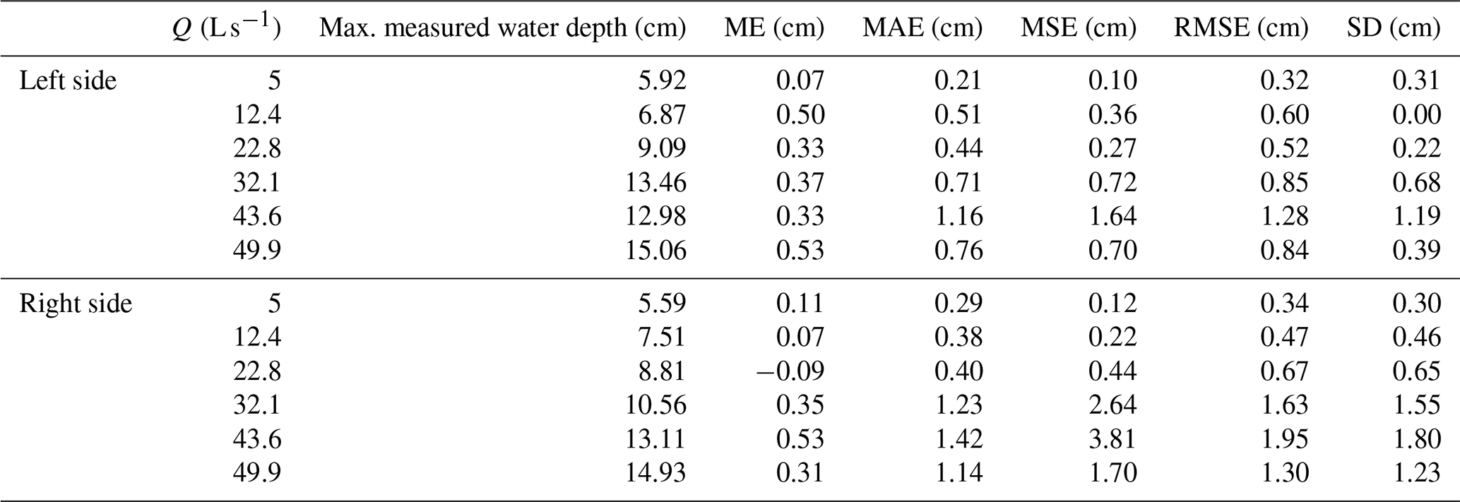
Table 1Error indices of the simulated water surface elevations at both sides.
2.3 Model verification
We conducted both a grid independence test and a comparison between the simulated and experimental results for model verification (Fig. 1). Grid independence was reached when the grid size of 0.25 cm was used for the main computation domain. Two measurements (Fig. S3 in the Supplement) in the previous flume experiments (Zhang et al., 2018, 2020) were used to validate the numerical models: (i) longitudinal water surface profiles extracted from the side cameras and (ii) the boundary between the jet and recirculation cell at the water surface recorded in pictures by the top view camera. Both measurements were extracted at the frequency of 2 Hz for 60 s. The mean error (ME), mean absolute error (MAE), mean square error (MSE), root mean square error (RMSE), and standard deviation (SD) were calculated for the differences between the simulations and measurements from the side views (Table 1) and the top views (Table S1 in the Supplement). The max RMSE of the simulated water surface was below 2 cm for side views (Table 1) and smaller than 3 cm for the boundaries between the jet and jump components from the top views (Table S1). The comparisons between simulated results and the measurements showed that the combined approach succeeded in capturing the flow characteristics for a step-pool feature built in the physical flume. See Sect. S1 in the Supplement for details of model verification.
2.4 Data processing
The kinetic energy (KE), turbulent kinetic energy (TKE), and turbulent dissipation (εT) were used in the analysis of turbulent features and transformation of flow energy in the step-pool unit. The turbulent dissipation was obtained when solving the RNG k−ε turbulence model, whereas the kinetic energy and turbulent kinetic energy were calculated by Eqs. (1) and (2) in the solver.
Here u denotes the instantaneous velocity and the subscripts denote the respective coordinate axis.
Here u′ denotes the instantaneous velocity fluctuation.
The Q criterion (Hunt et al., 1988; Flow science, 2016) was used to identify the coherent flow structures in the step-pool unit and the Qcriterion was calculated by Eq. (3) in FLOW3D. We used a threshold value of 1200 for Qcriterion to isolate coherent vortices in this study.
Here Ωij and Sij are the antisymmetric and symmetric parts of the velocity gradient tensor, respectively.
The shear stress and total pressure for the mesh grids on the bed surface were obtained from the solver. The shear stress was used directly in the analysis, while the total pressure (Pt) was further processed to obtain the dynamic pressure (Pd) by Eq. (4). Pd was used instead of Pt to highlight the spatial distribution of flow kinetic energy rather than the water depth distribution, especially in the pool area where water depth was relatively large.
Ps is the static water pressure, ρ is the water density at 20 ∘C of 1000 kg m−3, g is gravity acceleration, and h is the water depth at a horizontal location obtained from the solver.
The drag (FD) and lift (FL) forces acting on the step stones in the sampling volumes (Fig. 1) were also provided by the solver as the components of flow forces in the X and Z directions. Drag (CD) and lift (CL) coefficients for FD and FL were calculated by Eqs. (5) and (6), respectively.
U∞ is the approach velocity and A⊥ is the upstream projected area of the step stone in each sampling volume. The cross-section-averaged flow velocity at the upstream face of a sampling volume was used as the approach velocity, U∞.
When calculating the cross-section-averaged turbulent kinetic energy (TKE) for the recirculation vortices at the step toe and near the water surface separately, we used a threshold method to distinguish the areas occupied by them as follows. Since the TKE in the high-speed flow was far lower than that in the recirculation cells (see details in Sect. 3.1.2), the threshold slightly higher than the maximum of TKE in the high-speed flow was used to detect the boundaries of the vortices with the high-speed flow in each vertical line in a cross-section. After all the vertical lines in a cross-section were processed, the areas occupied by the vortices in each cross-section were obtained, together with the integral of TKE in these areas. These two parameters were then used to calculate the section-averaged TKE. As this threshold method only worked for the cross-sections where the recirculation cells are clearly separated by the jet, the calculation stopped at the cross-sections a bit upstream of the pool bottom for each discharge.
The spatial distributions of both hydraulic characteristics and flow forces in the step-pool unit are exhibited in this section, with most of the results presented using the time-averaged values of the processed data. To clearly present these distributions, only the scenarios under the two largest discharges (Q = 43.6 and 49.9 L s−1) are shown in most of the analysis, while the rest are shown in Sect. S2 in the Supplement. These two discharges were chosen for two reasons: (i) well-defined pool morphology showed up under the two flow conditions, and (ii) the scenario at 49.9 L s−1 recorded the topographic and hydraulic characteristics closest to the failure of this step-pool unit in the experiment and may present clues to the failure mechanism.
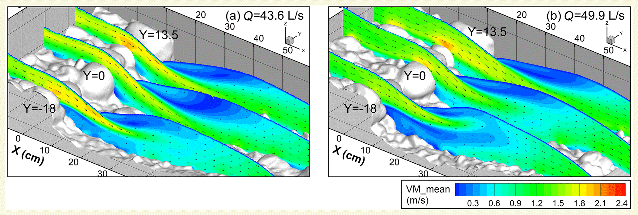
Figure 4Distribution of time-averaged velocity magnitude (VM_mean) and vectors in three longitudinal sections. The section at Y = 0 cm goes across the keystone, while the other two (Y = −18 and 13.5 cm) are located at the step stones beside the keystone. The spacing for the X, Y, and Z axes is 10 cm in the plots.
3.1 Flow properties
3.1.1 Mean flow velocity
The distribution of time-averaged flow velocity magnitude in three longitudinal sections is presented in Fig. 4, with the distribution of the Froude number shown in Fig. S8 in the Supplement. Flow accelerates and water depth decreases over the step stones before plunging into the pool as a jet feature. As a result, the Froude number reaches its maximum at the step crest (Fig. S8). The highest flow velocity in the vertical profile at the crests of step stones mainly exists near the stone surface (Fig. 4), different from the vertical profile of flow velocity upstream of the step for which the flow velocity is higher near the water surface (at 43.6 L s−1) or shows relatively uniform distribution (at 49.9 L s−1). The points of separation of the jet from the step face were located in the downstream parts of the step stones in the three sections.
The pool area under the two flow conditions exhibits highly nonuniform flow fields in all three longitudinal sections before the flow starts to accelerate on the negative slope (Fig. 4): low-velocity magnitudes close to 0 in a recirculation cell near the water surface associated with a hydraulic jump, low flow velocities at the step toe associated with an attached vortex, and high flow velocities (generally > 1 m s−1) in the jet between the two low-speed regions. It is worth noting that the jet impinges at the bed surface in the pool in the section Y = 0 and 13.5 cm but does not hit the bed in the section Y = −18 cm even though distinct scour also occurs near this section. The jet is separated from the bed by the vortex formed at the step toe in the section Y = −18 cm, in which the vortex at the step toe extends further downstream than that in the other two sections and then merges with the jet on the negative slope. The comparison among the three sections indicates that highly three-dimensional flow structures in step-pool features exist. The larger discharge and water depth at Q= 49.9 L s−1 result in the contraction of the recirculation cell near the water surface in the three sections but an expansion of the vortex at the step toe in the section Y = −18 cm compared with the case at Q = 43.6 L s−1. The jet penetration angles into the pool decrease in all three sections as the flow rate and water depth increase to 49.9 from 43.6 L s−1.
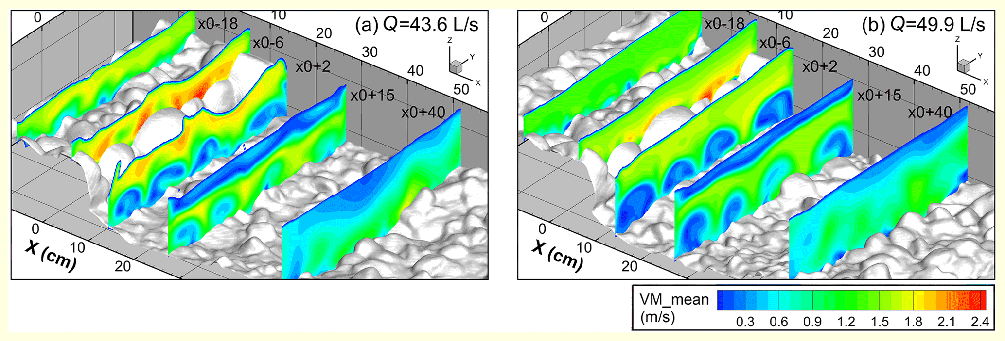
Figure 5Distribution of time-averaged flow velocity at five cross-sections which are set according to the reference section (x0). The reference cross-section x0 is located at the downstream end of the keystone (KS). The five sections are located at 18 and 6 cm upstream of the reference section (x0-18 and x0-6) and 2, 15, and 40 cm downstream of the reference section (x0+2, x0+15, x0+40). The spacing for the X, Y, and Z axes is 10 cm in the plots.
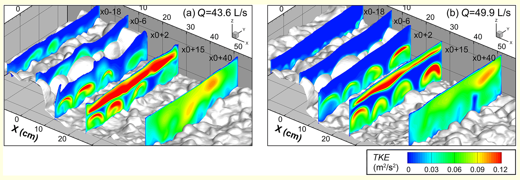
Figure 6Distribution of the time-averaged turbulence kinetic energy (TKE) at the five cross-sections described in Fig. 5.
The transverse distribution of flow velocity magnitude is presented in Fig. 5, with five cross-sections from the upstream to the downstream side of the step-pool model shown. Section x0-18 is located upstream of the step for which no distinct bed structures have developed. The water surface is relatively flat and velocity magnitude is relatively uniformly distributed in this section. The x0-6 section, which is located at the step crest, shows that the highest flow velocity is located above the no. 2 and 3 step stones (Fig. 3d), which are among the lowest points within the step crest. The section at x0+2 cm is located upstream of the contraction section for flow rates > 12.4 L s−1 and shows the existence of vortex cells at the step toe with transverse axes separated by regions of high-speed flows. The centers of the vortices follow the low points within the step crest (i.e., the contact points between step stones, while the high-speed flows correspond to the high points of the crests of the four step stones between the bank stones). In the section at x0+15 cm near the pool bottom at Q = 32.1, 43.6, and 49.9 L s−1, the vortices near the bed surface are less pronounced and show reduced velocity differences with the high-speed flows if compared with the section at x0+2 cm. The flow recirculation cell near the water surface with flow velocities close to 0 covers almost the entire flume width at this section. As a result, high-velocity magnitude appears in the middle of the vertical profile in most areas of this section. The section at x0+40 cm is located on the negative slope and shows no sign of the vortices near the bed. The recirculation cell near the water surface extends to this section but occupies only part of the flume width. The flow velocity becomes relatively uniform beneath the recirculation cell near the water surface compared to section x0+15. As the discharge increases from 43.6 to 49.9 L s−1, water depth increases in all five cross-sections, while the areas occupied by the flows > 1.8 m s−1 decrease in sections x0-6 and x0+2. The vortices formed at the toe of the step expand their areas in the sections x0+2 and x0+15 to 49.9 from 43.6 L s−1.
3.1.2 Turbulence
Figure 6 presents the transverse distribution of turbulence kinetic energy (TKE) in the same cross-sections as those in Fig. 5. The TKE upstream of the step (section x0-18) and at the step (section x0-6) is generally lower than in the pool. These areas of low TKE coincide with areas of high mean flow velocity (Fig. 5), indicating that mean flow velocity and TKE are inversely correlated.
Like mean flow velocity, the distribution of TKE in the pool also exhibits high nonuniformity at the highest flow conditions. Upstream of the contraction section (near section x0+2), high TKE is only located at the step toe within the attached vortices, while the jet with high flow velocity shows low turbulent energy near the water surface. Around the deepest area in the pool (section x0+15), the recirculation cells at both the water surface and the toe of the step show high turbulent energy, although that in the recirculation cell above the jet is much higher if we further compare the TKE level of both. In the section x0+40 on the negative slope, the turbulent energy decreases from the water surface to the bed surface in the vertical direction. For the recirculation cells near both the water surface and bed surface, the highest TKE values occur near the interfaces with the high-speed flow (e.g., section x0+15) owing to high fluid shear in these regions. The increase in flow rate from 43.6 to 49.9 L s−1 leads to the significant reduction of the TKE level near the bed surface in sections x0-18 and x0-6 upstream of the step and in the high-speed flows in the pool (e.g., sections x0+2 and x0+15).
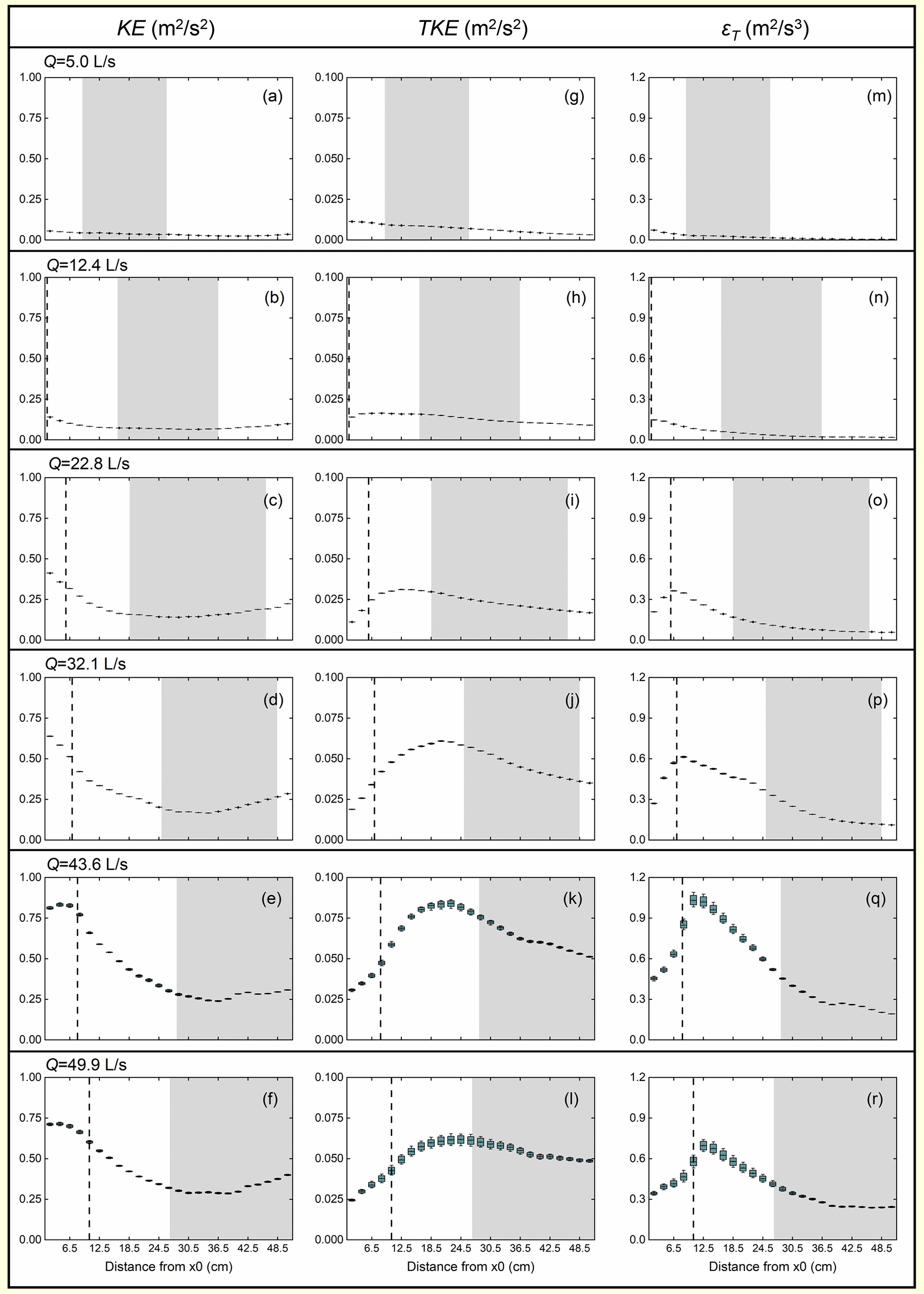
Figure 7Box plots for the distributions of the mass-averaged flow kinetic energy (KE, panels a–f), turbulence kinetic energy (TKE, panels g–l), and turbulent dissipation (εT, panels m–r) in the pool over 30 s for all six tested discharges (the plots at the same discharge are in the same row). The mass-averaged values were calculated every 2 cm in the streamwise direction. The flow direction is from left to right in all the plots. The general locations of the contraction section for all the flow rates are marked by the dashed lines, except for Q = 5 L s−1 when the jump is located too close to the step. The longitudinal distance taken up by negative slope for the inspected range is shown by the shaded area in each plot.
To present the transformation of flow energy in the pool, we plot the longitudinal distribution of mass-averaged KE, TKE, and εT downstream of the section x0 in Fig. 7. The key findings are as follows.
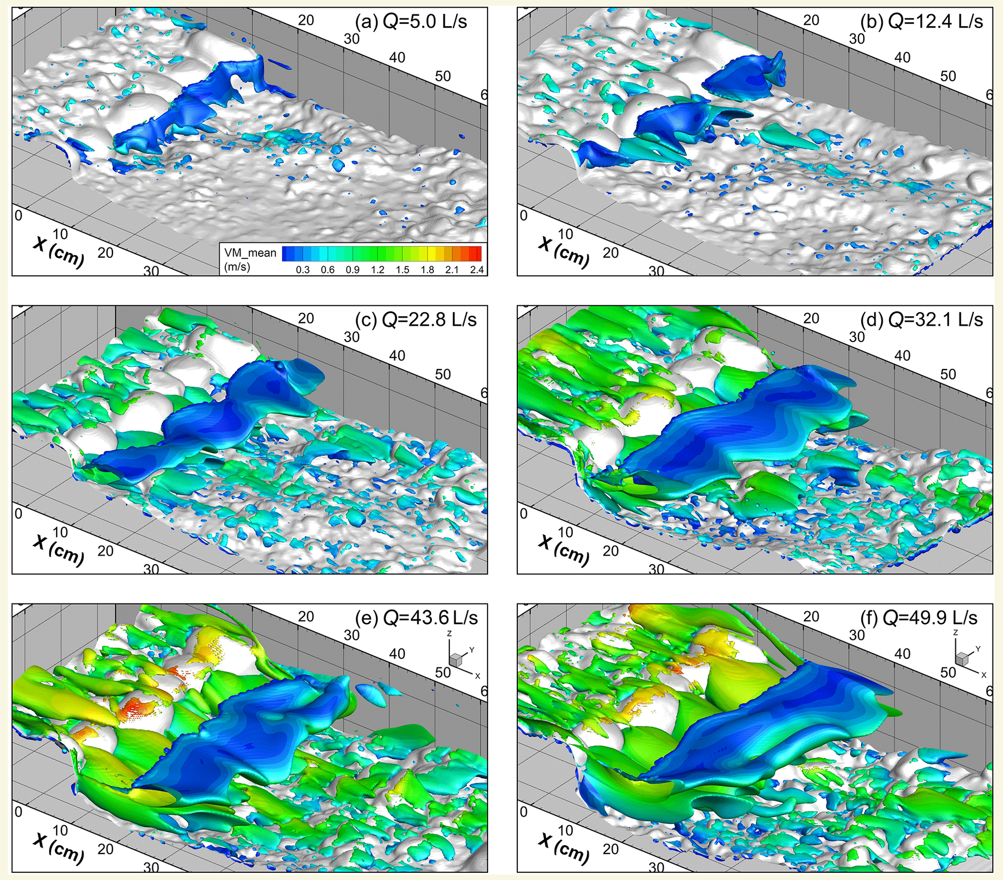
Figure 8Instantaneous flow structures extracted using the Q criterion (Qcriterion = 1200) and colored by the magnitude of flow velocity.
First, at all the discharges examined, the KE decreases after flow plunges into the pool but shows a slightly increasing trend on the negative slope (Fig. 7a–f). It is worth noting that at the two highest discharges (Fig. 7e and f), the flow kinetic energy remains at a high level at a distance of 5–6 cm downstream of x0, which is occupied by the jet feature before it decreases dramatically where the jump starts. Second, the TKE first increases in the pool, reaches the maximum around the pool bottom, and then decreases on the negative slope (Fig. 7g–l). The location of the maximum of TKE moves further downstream as flow increases, during which pool scour keeps developing and the pool bottom area also moves downstream (Zhang et al., 2020). Third, εT increases sharply downstream of x0 and reaches the maximum earlier than the TKE in the pool. The turbulent dissipation rate on the negative pool slope remains at a low level, even lower than that near the step toe (Fig. 7m–r). Fourth, the maximum value of KE, TKE, and εT in the pool increases during a flow increase from 5.0 to 43.6 L s−1 but decreases when the flow further increases to 49.9 L s−1 with intensified pool scour.
3.1.3 Coherent flow structure
The instantaneous turbulent structures are presented in Fig. 8 (front view shown in Fig. S12 in the Supplement). Upstream of the step, coherent structures are mainly streamwise and located near the bed, particularly downstream of protruding grains at the flow rate higher than 12.4 L s−1. Rich coherent structures exist downstream of the step in both the flow recirculation cell of the jump that stretches across the entire channel width near the water surface and the discrete vortices extending along the streamwise direction attached to the step toe close to the bed. The dimensions of the vortex structures near both the water and bed surfaces expand as the flow rate increases and pool scour develops. No clear coherent structures are visualized in the high-speed flow region in the pool, indicating low vorticity there. The vortices at the step toe start at the contact point of two neighboring step stones, and their widths and heights decrease downstream until the vortices vanish near the start of the negative slope. On the negative slope, coherent structures mainly follow protruding grains (micro-scale bed structures) but are not elongated in the streamwise direction as they are upstream of the step, even though the grain sizes are similar.
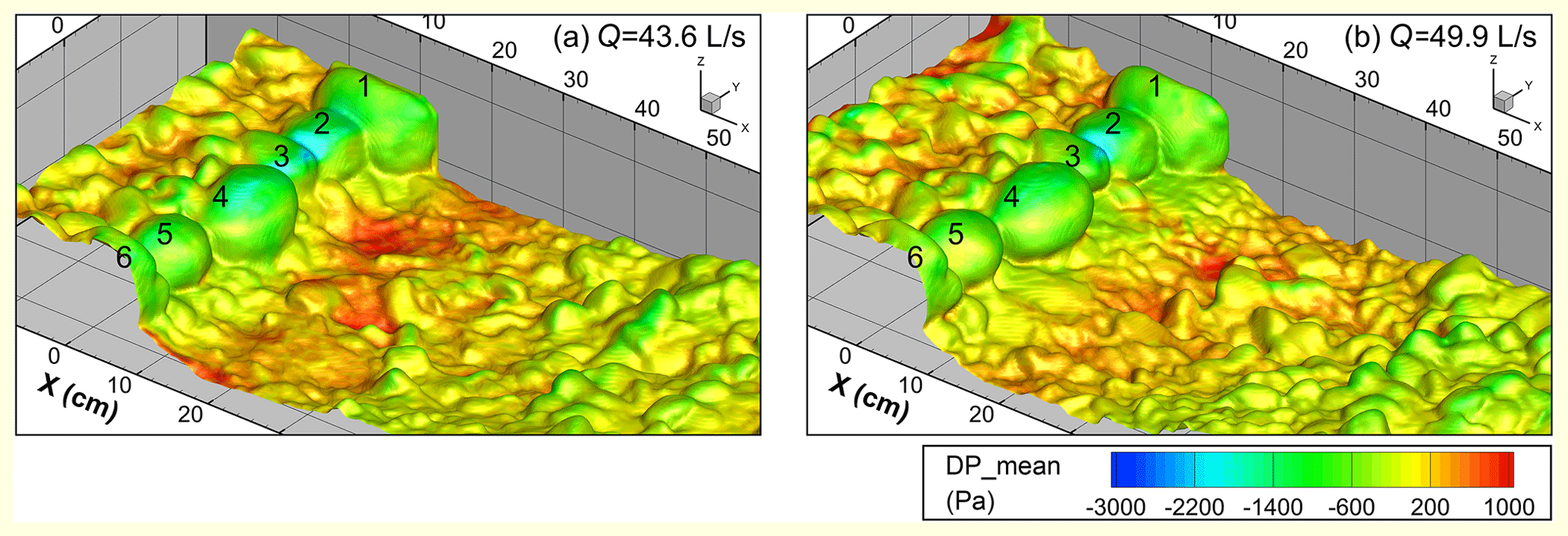
Figure 9Time-averaged dynamic pressure (DP_mean) on the bed surface in the step-pool model under the two highest discharges, with the step numbers marked. The negative values in the plots result from the setting of standard atmospheric pressure to 0 Pa, the absolute value of which is 1.013 × 10⁵ Pa.
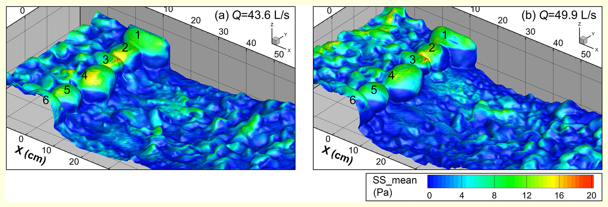
Figure 10Time-averaged shear stress (SS_mean) on the bed surface in the step-pool model, with the step numbers marked. The standard atmospheric pressure is set as 0 Pa.
3.2 Flow forces
3.2.1 Dynamic pressure
For all the flow conditions, the dynamic pressure is at a relatively low level on the step stones and becomes even lower at the points of flow separation of the jet from the step face. The dynamic pressure on the step stones generally decreases with the increase in flow rate and development of pool scour. The minimum of dynamic pressure appears at the contact between no. 2 and 3 stones at high flows (Fig. 9) where the highest flow velocity is located within the step crests (Fig. 5). Relatively high dynamic pressure exists near the points impinged by the high-speed jet in the pool, and its magnitude generally increases with flow rate (Figs. 9 and S13 in the Supplement). The dynamic pressure at the pool bottom shows higher values at Q = 43.6 L s−1 than Q = 49.9 L s−1, although the scour depth is larger at Q = 49.9 L s−1. This is related to the lower water depth in the pool but the higher flow velocity of the jet at Q = 43.6 L s−1 (Figs. 4 and 5). The front sides of the protruding grains or grain clusters to the flow on the negative slope show significantly lower dynamic pressures than on the back sides and surrounding grains.
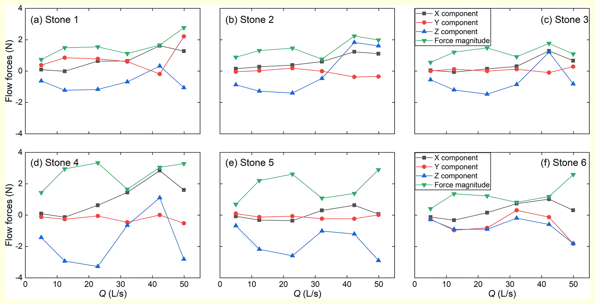
Figure 11Variation of fluid force components and magnitude of resultant flow force acting on step stones with flow rate. Stone 4 is the keystone. Stone numbers are consistent with those in Figs. 9 and 10. The upper limit of the sampling volumes for flow force calculation is higher than the water surface, while the lower limit is set at 3 cm lower than the keystone crest.
3.2.2 Shear stress
As shown in Fig. 10, the magnitude of shear stress along the step-pool model is generally 2 orders of magnitude smaller than that of the dynamic water pressure. The highest values of shear stress occur on the crests of the step stones. The shape and maximum height of the step stones influence the distribution of shear stress significantly. The no. 2 and 3 stones with relatively flat and low crests show higher shear stress at the contact of these two stones but quite low (close to 0) shear stress on the downstream faces. In contrast, the shear stress on the no. 4 (KS) and 5 stones, which have an ellipsoid shape, reaches a maximum near the highest point of each stone. There is also a high-shear-stress zone on the downstream faces of these two step stones with a downstream curvature. The downstream curvatures of the high-shear-stress zones on the step stones match the boundary of the step toe vortices well (Fig. 8). Shear stress also shows higher values where the bed is impinged by the jet as well as on some protruding clusters and grains on the negative slope.
3.2.3 Flow forces on step stones
The variations of the components of flow forces on each step stone reveal the following patterns (Fig. 11). First, the component in the X direction, i.e., the drag force, on all the step stones increases until the flow rate reaches 43.6 L s−1 but decreases when the flow is further increased to 49.9 L s−1. The keystone (stone 4), which was the first stone to move and triggered the step failure in the Zhang et al. (2020) experiment, has the largest drag force at high flows. Second, the component in the Z direction of flow force, i.e., the lift force, generally has a larger magnitude than the drag force on step stones before the flow rate reaches 43.6 L s−1. The lift force on the stones 1–4 changes direction from downward to upward at Q = 43.6 L s−1, when flow velocity significantly increases at the step but the water depth is similar to that at Q = 32.1 L s−1 (Figs. 4 and S9 in the Supplement). When the discharge is further increased to 49.9 L s−1 and water depth shows a clear increase (Figs. 4 and 5), the lift force changes direction to downward again. Third, the Y component on the step stones between the bank stones is about 2–3 orders of magnitude smaller than the components in the other two directions. In contrast, the Y component of flow force has the largest magnitude of any component for the two bank stones at the highest flow. This indicates that the transverse interaction between the step and the flow mainly occurs at the banks. Lastly, the magnitude of the resultant flow force increased when the discharge reached 49.9 L s−1 for the step stones except for stones 2–3, where the flow velocity is the greatest.
Both the drag and lift coefficients generally increase for all the step stones for the discharges from 12.4 to 43.6 L s−1 and decrease slightly for stones 3–6 when the discharge is further increased to 49.9 L s−1 (Fig. S15c–f in the Supplement). However, the magnitude of CL remains significantly larger than CD at most flow rates for all the step stones, resulting in the greater variation of CL that coincides with discharge increase.
4.1 Three-dimensionality of flow characteristics
Using the combined approach, we provided a detailed description of the 3D flow properties at a millimeter resolution around a step-pool unit made of natural gravels for the first time. Based on the results of this study, well-developed three-dimensionality of the flow structures in the pool is revealed: the vortices formed at the step toe are discrete structures along the streamwise direction, as distinct from the recirculation cell near the water surface as an integrated flow structure covering the entire flume width (Figs. 8 and S12 in the Supplement). Natural grains used to build the step-pool unit with randomness and irregularity in size, shape, and orientation result in a 3D topography for the step (Fig. 2a). Our results show that the emergence of vortices at the step toe is related to the lower points in the step crests, while the higher points of step crests generate a jet with enough momentum to hit the bed surface directly. Wilcox et al. (2011) noticed the possible influence of the variability in step architecture on the distribution of hydraulics and turbulence as well as the flow resistance of a step-pool sequence. Our results further reveal that the transverse configuration of a boulder step influences the flow characteristics of the downstream pool in a significant way.
A jet that hits the bed is defined as an impinging jet, while it is defined as a surface flow if it remains at the water surface after plunging (Wu and Rajaratnam, 1998). The general jet regime for the whole step structure was recognized as an impinging jet in the CIFR T2 run (Zhang et al., 2020) based mainly on the water depths measured near the flume walls. However, the 3D flow structures show that the jet does not impinge the pool bottom in some longitudinal sections (Figs. 4 and 5). Our results illustrate the limitation of measurements at the flume walls and highlight the great advantage of the combined approach in presenting fully resolved 3D hydraulic information over complex topography. The 3D flow structures visualized by the combined approach indicate that the flow regime over a step-pool unit is not necessarily binary (i.e., either impinging jet or surface flow) and that the flow regime at Q = 49.9 L s−1 is probably transitional between the impinging jet and surface flow regimes.
Our results also illustrate the segmentation of flow velocity and turbulence in the pool: recirculation cells with low flow velocity but high TKE near the water surface as well as close to the step toe and high-speed flow with low TKE between the recirculation cells. This segmentation remains until the flow reaches the negative slope (Figs. 4 and 5). The intense mid-profile fluid shearing within the hydraulic jump and between the flow recirculation cells at the step toe and the jet plunging over the step face generates high TKE levels in the pool (Fig. 6). In this sense, the 3D simulated results illustrate the context of the non-logarithmic vertical profiles of flow velocity and turbulence below steps measured in the field, which show higher flow velocity and turbulence in the middle of the profile (Wohl and Thompson, 2000; Li et al., 2014).
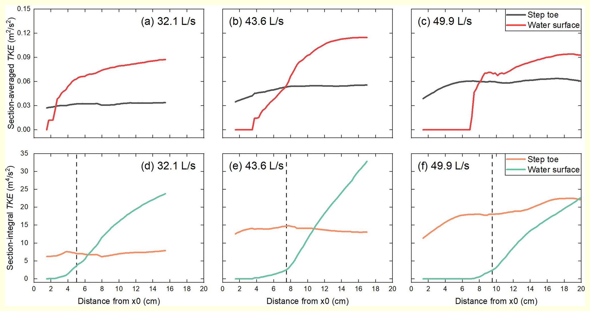
Figure 12Longitudinal distributions of section-averaged and section-integral turbulent kinetic energy (TKE) for the flow recirculation cells at the step toe, near the water surface, and at the largest three discharges. The flow direction is from left to right in all the plots. The general locations of the contraction sections under the three flow rates are marked by dashed lines in (d) to (f).
4.2 Energy dissipation mechanism
Energy dissipation within a step-pool unit has been reported to mainly occur in the pool area (Wohl and Thompson, 2000; Li et al., 2014; Zhang et al., 2020). With the distribution of the flow velocity, kinetic energy, turbulent kinetic energy, and turbulent dissipation presented in detail by the combined approach (Figs. 5–7), we further visualize the energy dissipation mechanisms in the pool. The distributions of both TKE and εT in the pool exhibit high nonuniformity (Fig. 7). It is noteworthy that the energy transformation and dissipation are concentrated in the area upstream of the negative slope. The recirculation cells near both the water surface and the toe of the step show much higher TKE than the high-speed flows in the pool (Fig. 6), suggesting that two energy dissipators, i.e., the two recirculation cells, co-exist upstream of the negative slope. The recirculation cell near the water surface has been recognized as the energy dissipator for a step-pool unit owing to its strongly fluctuating appearance (Church and Zimmermann, 2007; Wyrick and Pasternack, 2008; Wang et al., 2012; Zhang et al., 2018). However, little attention has been paid to the dissipation properties close to the step toe as most measurements would be blocked by the turbulent water surface. The combined approach makes it possible to compare the level of TKE in these two dissipators quantitatively. We calculated the section-integral and section-averaged (section-integral values divided by the areas taken by the two dissipators in the cross-section) TKE for each dissipator before these two dissipators get mixed, as shown in Fig. 12.
Downstream of the contraction section, no difference of order is found in the section-averaged or section-integral TKE between the flow recirculation cells near the water surface and formed at the step toe for the streamwise length examined here. This indicates that these two recirculation cells are comparable contributors for energy dissipation in the pool. It is worth noting that the TKE in the recirculation cell near the water surface decreases when the discharge is increased to 49.9 from 43.6 L s−1, whereas the TKE level in the vortex attached to the step toe sees a further increase. The suppression of TKE near the water surface at 43.6 L s−1 may be related to the higher submergence of the step and transition of jump regimes at higher flow conditions (Pasternack et al., 2006; Wyrick and Pasternack, 2008; Zhang et al., 2020). The increase in TKE close to the step toe is associated with the development of pool scour as the flow increases (Zhang et al., 2020). This contrast suggests that the contribution of the vortices formed at the step toe to the total energy dissipation increases with flow increase and pool development at high discharges.
The step-pool morphology has been reported to show a higher capacity of flow energy dissipation than a vertical drop with the same height (Zhang et al., 2020). The new understanding of the energy dissipation mechanism for step-pool features may provide two explanations for this phenomenon. First, the 3D natural step structure leads to 3D configurations of vortices formed close to the step toe, and the interface between energy dissipators and the high-speed flow is enlarged. As the interfaces are where high TKE occurs (Fig. 6), the energy loss of the flow in the 3D vortices at the step toe may surpass that of the 2D recirculation vortices below a drop. Second, the pool geometry in a step-pool unit is normally more complex than in an artificial pool, and the pool scour is intensified with flow increases until the step structure collapses (Comiti et al., 2005; Church and Zimmermann, 2007; Zhang et al., 2018, 2020). This morphological evolution maintains the co-existence of two energy dissipators for a step-pool unit and enlarges the energy capacity of the vortices at the step toe with increases in flow. In contrast, the fixed rectangular shape of an artificial 2D drop results in significant suppression of the recirculation cell near the water surface and limited space for the recirculation vortex to expand at the step toe, especially under skimming flow conditions (Chanson, 2001).
4.3 Interaction between hydraulics and morphological evolution
The distributions of flow velocity (Figs. 4 and 5), TKE (Figs. 6 and 7), and coherent structure (Fig. 8) in the pool have demonstrated the expansion of the recirculation cells both near the water surface and at the step toe with the development of pool scour and flow increase up to the discharge of 43.6 L s−1. The expansion of the recirculation cell near the water surface presented by the combined approach is generally consistent with the experimental observations (Zhang et al., 2020). The results of this study further illustrate that both the geometric dimensions and TKE of the recirculation cell near the water surface decrease when the discharge is increased to 49.9 from 43.6 L s−1 (Figs. 4–6, and 12). This indicates that the increase in the submergence of the step would suppress the flow recirculation cell of the hydraulic jump at high flows. In contrast, the vortices at the step toe show an increase in geometric dimensions and TKE with this flow increase (Figs. 5, 6, 8, and 12). This difference in response to the discharge increase to 49.9 L s−1 results from the change in jet penetration angle due to the increase in water depth (Fig. 4). The decrease in jet penetration angle at Q = 49.9 L s−1 also leads the pool bottom to move downstream, which creates space for the vortices to expand downstream of the step toe. The expansion of the vortices at the step toe together with the relatively low flow velocity and high turbulence within these vortices may explain the increased deposition of fine sediment at the step toe at Q = 49.9 L s−1 (Zhang et al., 2020). The number and location of vortices attached to the step toe remain almost unchanged during this process. This is related to the stable architecture of the step structure, which determines the distribution of jet angle and momentum at the step crest.
Apart from the pool scour, the development of micro-bedforms in the form of grain clusters, which are mainly located at the pool bottom and on the negative slope (Figs. 9 and 10), is another noteworthy morphological variation of the step-pool feature (Zhang et al., 2020). The high-spatial-resolution outputs of the combined approach allow us to inspect the interaction between the grain clusters and pool hydraulics. The grain clusters at the pool bottom are mainly located where the bed is impinged by the jet rather than in the areas occupied by the recirculation cells connected to the step toe (Figs. 10 and S14 in the Supplement). These grain clusters have very limited disturbance on the surrounding flow field (see details in Sect. S3 in the Supplement). The grain clusters on the negative slope where the jet and recirculation cells lose their identity (Figs. 4–6) do not show any distribution patterns but increase the flow velocity and turbulence above them significantly (Figs. S16 and S17 in the Supplement). These grain clusters also have clearer coherent structures in their wake zones than those located at the pool bottom, and these small-scaled coherent structures expand as the pool scour develops (Fig. 8). In summary, the distribution of micro-bedforms at the pool bottom is affected by the jet, while the micro-bedforms on the negative slope create strong interference in the surrounding hydraulics where the jet merges with the recirculation cells.
4.4 Implications for stability and failure of step-pool features
The distributions of dynamic pressure and shear stress show that the step structure bears the lowest dynamic pressure but highest shear stress in the step-pool unit and that the distributions of water forces on the step stones are significantly affected by the stone sizes and shapes (Figs. 9 and 10). The drag force on the step stones generally increases with flow rate except when flow is increased to 49.9 from 43.6 L s−1 (Fig. 11). The step structure collapsed owing to the movement of the KS soon after the flow discharge was further enhanced from 49.9 L s−1 in the flume experiment (Fig. 2b, Zhang et al., 2020). This implies that triggers for the movement of the KS apart from the increase in drag force (Lenzi, 2002; Weichert, 2005) may also exist. The lift force on the step stones shows a much larger variation range compared to the drag force (Fig. 11), and the magnitude of the lift coefficient is also larger than the drag coefficient generally (Fig. S15). The direction of the lift force may also change during flow increase (Fig. 11a–d). The highly variable lift coefficient and lift force observed in this study might partly be the result of using only the protruding part of each step stone in force analysis (Fig. 3d) but are also consistent with the experimental finding on submerged particles on a rough planar gravel bed in Lamb et al. (2017). The comparison between the drag and lift forces implies that the vertical component of flow force might play an important role in the mobility of step stones. The variation of lift forces will lead to the variation in the forces on the step stones from the contacting coarse grains in bed materials (Zhang et al., 2016) before the step-pool failure. This variation of the reactive forces might result in subtle changes in the internal structures of the bed material grains beneath step stones, e.g., reconfiguration of gaps between coarse particles and distribution of fine sediment in these gaps (Gibson et al., 2011). The internal structure has been found to be closely related to the structural deformation and the final failure of the step (Zhang et al., 2018). Therefore, we infer that the variation of lift force on step stones and surrounding grains might also affect step stability and is worthy of further investigation in future research. We also admit that the data for step-pool failure are very limited in this study, and solid conclusions related to the failure mechanism can only be reached with further inspection of the flow forces at more step-pool failures.
4.5 Limitations of the combined approach
Although the combined approach shows great advantages in obtaining high-resolution information on the 3D flow properties for a step-pool unit, this approach also has limitations that merit consideration in future research.
-
The bed surface is set to be impermeable in the CFD model. This setting results mainly in two inconsistencies with reality. First, the hyporheic flow in a step-pool unit has been neglected. Hyporheic flow beneath the step-pool unit has been reported to exit the bed near the step toe (Hassan et al., 2015), which may affect the vortices formed here to some degree. Second, the upstream sides of step stones beneath the bed surface are also submerged by water owing to the high porosity of bed materials (Zhang et al., 2016, 2018) and hence also experience water pressure. Without considering this pressure in our model, the drag force on the step stones would be heavily biased, i.e., pointing upstream in most cases. Consequently, only parts of step stones above the upstream bed surface were analyzed (Fig. 3d). When further information on the 3D internal structure beneath the bed surface is accessible, hyporheic models (e.g., Dudunake et al., 2021) could be added to the CFD simulation to resolve this limitation.
-
No consideration for air entrainment in recirculation cells associated with the jump regime which was observed during the flume experiment (Zhang et al., 2018, 2020) is taken. Aeration has been reported to affect the flow velocity and turbulence properties downstream of a natural step (Vallé and Pasternack, 2006). Neglecting the air entrainment may be the reason for the mismatch between the simulated results and hydraulic measurements around the jump (Figs. S4–S6 in the Supplement) as a high air concentration would increase the jump volume (Lenzi et al., 2003). However, no measurement of air concentration in the jump was collected in the flume experiment for us to set parameters and validate the aeration module which could be coupled to the CFD model. Also, adding an aeration module might reduce the computational stability but increase computation cost in our case.
-
The topographic models of the bed surfaces contain limited areas upstream of the step owing to the measuring difficulty. This limitation might result in the underestimation of turbulence development upstream of the step-pool model. However, considering that the bed-generated turbulence is greatly suppressed upstream of step structure at high flows (e.g., Fig. 6; Wohl and Thompson, 2000), the errors caused by the limited area are acceptable. A long enough distance from the inlet to a step-pool unit is suggested for future research to better reconstruct the incoming flow turbulence for the step-pool unit.
-
The RNG k−ε turbulence model and first-order momentum advection were applied in the CFD simulation. Such settings ensured computational stability for the flow over the highly complex bed surface of a step-pool unit but led to a loss in numerical accuracy and hence could only provide time-averaged results. As a result, this study can only focus on the spatial distribution rather than the temporal distribution of hydraulic features for a step-pool unit. The performance of a higher-order approach for step-pool features remains an open research question for future research.
-
Only one step-pool unit instead of step-pool sequences was built and tested in the experiments of Zhang et al. (2020) due to lab limitation and the study focus of isolating one step-pool unit. However, step-pool features mainly appear in sequences in nature. The possible differences in hydraulics between one single step-pool unit and step-pool units in sequence remain to be explored in future.
In this study, we developed a combined approach, which utilizes flume experiments and CFD modeling, to resolve the detailed 3D flow characteristics for a step-pool unit made of natural stones. The main findings of this study are as follows.
First, the most prominent feature of hydraulics in the pool is the segmentation of flow velocity upstream of the negative slope, which consists of the recirculation cell near the water surface, streaky vortices formed close to the step toe, and high-speed flow in between. The transverse configuration of a boulder step significantly affects the flow characteristics downstream. Second, the distribution of TKE in the pool is highly nonuniform, with the concentration of flow energy transformation and dissipation upstream of the negative slope in the pool. Both the recirculation cells at the water surface and step toe are the main energy dissipators for a step-pool unit with a well-defined pool configuration. Third, the development of pool scour and flow increase result in an increase in volume and turbulence energy in the recirculation cells in the pool before the recirculation cell at the water surface is suppressed at the highest flow. The interference of the micro-bedforms on the surrounding hydraulics is small where the vortices attached to the step and jets dominate in the pool but is greater on the negative slope. Finally, the step experiences the lowest dynamic pressure but highest shear stress in the step-pool unit. The drag force on the step stones generally increases with discharge; however, it decreases when the discharge reaches the critical value to destabilize the step structure. Compared with the drag force, the lift force on step stones shows a larger magnitude and a much wider variation when flow is increased.
The combined approach, despite its intrinsic limitations (e.g., using an impermeable bed surface in the model), has shown great advantages in capturing fully resolved 3D hydraulic information over merely using flume experiments. The advanced hydraulic information obtained using this approach helps in achieving a comprehensive understanding of the interaction between hydraulics and morphology as well as mechanisms of energy dissipation and stability for step-pool features.
Topographic models of the step-pool unit recognized in the CFD models and key settings of the CFD models can be found at https://doi.org/10.5281/zenodo.5840753 (Zhang, 2022).
The supplement related to this article is available online at: https://doi.org/10.5194/esurf-10-1253-2022-supplement.
CZ conceptualized and designed the research, processed the measurements of flume experiments, performed the numerical simulations, analyzed the data, wrote the paper, prepared the figures, and contributed to funding acquisition. YX significantly contributed to the conceptualization of the work, provided key advice in the numerical simulations, and reviewed several versions of the paper. MAH contributed to the design of the research, reviewed and edited several versions of the paper, and significantly contributed to the interpretation and contextualization of the results. MX greatly contributed to funding acquisition and arrangement of resources, provided advice on research design, and reviewed the paper. PH contributed by performing numerical simulations, verifying the model, analyzing the data, and preparing the figures and paper.
The contact author has declared that none of the authors has any competing interests.
Publisher's note: Copernicus Publications remains neutral with regard to jurisdictional claims in published maps and institutional affiliations.
Yingjun Liu from Tsinghua University is kindly acknowledged for his assistance in processing topographic models of bed surface and establishing the early versions of the CFD models.
This study is supported by the National Natural Science Foundation of China (nos. 51779120, 52009062, 41790434), the Strategic Priority Research Program of the Chinese Academy of Sciences (XDA23090401), and the Open Research Fund Program of the State key Laboratory of Hydroscience and Engineering, Tsinghua University (sklhse-2021-B-03).
This paper was edited by Jens Turowski and reviewed by Keith Richardson and one anonymous referee.
Adrian, R. J.: Twenty years of particle image velocimetry, Exp. Fluids, 39, 159–169, https://doi.org/10.1007/s00348-005-0991-7 2005.
Bayon, A., Valero, D., García-Bartual, R., and López-Jiménez, P. A.: Performance assessment of OpenFOAM and FLOW-3D in the numerical modeling of a low Reynolds number hydraulic jump, Environ. Modell. Softw., 80, 322–335, https://doi.org/10.1016/j.envsoft.2016.02.018, 2016.
Bayon, A., Toro, J. P., Bombardelli, F. A., Matos, J., and López-Jiménez, P. A.: Influence of VOF technique, turbulence model and discretization scheme on the numerical simulation of the non-aerated, skimming flow in stepped spillways, J. Hydro-Environ. Res., 19, 137–149, https://doi.org/10.1016/j.jher.2017.10.002, 2018.
Chanson, H.: Hydraulic design of stepped spillways and downstream energy dissipators, Dam Eng., 11, 205–242, 2001.
Chartrand, S. M., Jellinek, M., Whiting, P. J., and Stamm, J.: Geometric scaling of step-pools in mountain streams: Observations and implications, Geomorphology, 129, 141–151, https://doi.org/10.1016/j.geomorph.2011.01.020, 2011.
Chen, Y., Liu, X., Gulley, J. D., and Mankoff, K. D.: Subglacial conduit roughness: Insights from computational fluid dynamics models, Geophys. Res. Lett., 45, 11–206, https://doi.org/10.1029/2018GL079590, 2018.
Chen, Y., DiBiase, R. A., McCarroll, N., and Liu, X.: Quantifying flow resistance in mountain streams using computational fluid dynamics modeling over structure-from-motion photogrammetry-derived microtopography, Earth Surf. Proc. Land., 44, 1973–1987, https://doi.org/10.1002/esp.4624, 2019.
Chen, Y., Bao, J., Fang, Y., Perkins, W. A., Ren, H., Song, X., Duan, Z., Hou, Z., He, X., and Scheibe, T. D.: Modeling of streamflow in a 30 km long reach spanning 5 years using OpenFOAM 5.x, Geosci. Model Dev., 15, 2917–2947, https://doi.org/10.5194/gmd-15-2917-2022, 2022.
Chiu, C. L., Fan, C. M., and Tsung, S. C. Numerical modeling for periodic oscillation of free overfall in a vertical drop pool, J. Hydraul. Eng., 143, 04016077, https://doi.org/10.1061/(ASCE)HY.1943-7900.0001236, 2017.
Church, M. and Zimmermann, A.: Form and stability of step-pool channels: Research progress, Water Resour. Res., 43, W03415, https://doi.org/10.1029/2006WR005037, 2007.
Cignoni, P., Callieri, M., Corsini, M., Dellepiane, M., Ganovelli, F., and Ranzuglia, G.: Meshlab: an open-source mesh processing tool, in: Eurographics Italian chapter conference, Salerno, Italy, 2–4 July 2008, 129–136, 2008.
Comiti, F., Andreoli, A., and Lenzi, M. A.: Morphological effects of local scouring in step-pool streams, Earth Surf. Proc. Land., 30, 1567–1581, https://doi.org/10.1002/esp.1217, 2005.
Dudunake, T., Tonina, D., Reeder, W. J., and Monsalve, A.: Local and reach-scale hyporheic flow response from boulder – induced geomorphic changes, Water Resour. Res., 56, e2020WR027719, https://doi.org/10.1029/2020WR027719, 2020.
Eltner, A., Kaiser, A., Castillo, C., Rock, G., Neugirg, F., and Abellán, A.: Image-based surface reconstruction in geomorphometry – merits, limits and developments, Earth Surf. Dynam., 4, 359–389, https://doi.org/10.5194/esurf-4-359-2016, 2016.
Flow Science: Flow-3D Version 11.2 User Manual, Flow Science, Inc., Los Alamos, 2016.
Gibson, S., Heath, R., Abraham, D., and Schoellhamer, D.: Visualization and analysis of temporal trends of sand infiltration into a gravel bed, Water Resour. Res., 47, W12601, https://doi.org/10.1029/2011WR010486, 2011.
Golly, A., Turowski, J. M., Badoux, A., and Hovius, N.: Testing models of step formation against observations of channel steps in a steep mountain stream, Earth Surf. Proc. Land., 44, 1390–1406, https://doi.org/10.1002/esp.4582,2019.
Hassan, M. A., Tonina, D., Beckie, R. D., and Kinnear, M.: The effects of discharge and slope on hyporheic flow in step-pool morphologies, Hydrol. Process., 29, 419–433, https://doi.org/10.1002/hyp.10155, 2015.
Hirt, C. W. and Nichols, B. D.: Volume of Fluid (VOF) method for the dynamics of free boundaries, J. Comput. Phys., 39, 201–225, https://doi.org/10.1016/0021-9991(81)90145-5, 1981.
Hirt, C. W. and Sicilian, J. M.: A porosity technique for the definition of obstacles in rectangular cell meshes, International Conference on Numerical Ship Hydrodynamics, 4th. Washington DC, USA, 24–27 September 1985.
Hunt, J. C., Wray, A. A., and Moin, P.: Eddies, streams, and convergence zones in turbulent flows. in: Proceedings of the 1988 summer program, Studying turbulence using numerical simulation databases, II, Standford, CA, 1 December 1988, 193–208, 1988.
Javernick L., Brasington J., and Caruso B.: Modeling the topography of shallow braided rivers using structure-from-motion photogrammetry, Geomorphology, 213, 166–182, https://doi.org/10.1016/j.geomorph.2014.01.006, 2014.
Lai, Y. G., Smith, D. L., Bandrowski, D. J., Xu, Y., Woodley, C. M., and Schnell, K.: Development of a CFD model and procedure for flows through in-stream structures, J. Appl. Water Eng. Res., 1–15, https://doi.org/10.1080/23249676.2021.1964388, 2021.
Lamb, M. P., Brun, F., and Fuller, B. M. Direct measurements of lift and drag on shallowly submerged cobbles in steep streams: Implications for flow resistance and sediment transport, Water Resour. Res., 53, 7607–7629, https://doi.org/10.1002/2017WR020883, 2017.
Lenzi, M. A.: Step-pool evolution in the Rio Cordon, northeastern Italy, Earth Surf. Proc. Land., 26, 991–1008, https://doi.org/10.1002/esp.239, 2001.
Lenzi, M. A.: Stream bed stabilization using boulder check dams that mimic step-pool morphology features in Northern Italy, Geomorphology, 45, 243–260, https://doi.org/10.1016/S0169-555X(01)00157-X, 2002.
Lenzi, M. A., Marion, A., and Comiti, F.: Local scouring at grade-control structures in alluvial mountain rivers, Water Resour. Res., 39, 1176, https://doi.org/10.1029/2002WR001815, 2003.
Li, W., Wang Z., Li, Z., Zhang, C., and Lv, L.: Study on hydraulic characteristics of step-pool system, Adv. Water Sci., 25, 374–382, https://doi.org/10.14042/j.cnki.32.1309.2014.03.012, 2014 (in Chinese with English abstract).
Maas, H. G., Gruen, A., and Papantoniou, D.: Particle tracking velocimetry in three-dimensional flows, Exp. Fluids, 15, 133–146, https://doi.org/10.1007/BF00223406, 1993.
Montgomery, D. R. and Buffington, J. M.: Channel-reach morphology in mountain drainage basins, Geol. Soc. Am. Bul., 109, 596–611, https://doi.org/10.1130/0016-7606(1997)109<0596:CRMIMD>2.3.CO;2, 1997.
Morgan J. A., Brogan D. J., and Nelson P. A.: Application of structure-from-motion photogrammetry in laboratory flumes, Geomorphology, 276, 125–143, https://doi.org/10.1016/j.geomorph.2016.10.021, 2017.
Morovati, K., Homer, C., Tian, F., and Hu, H.: Opening configuration design effects on pooled stepped chutes, J. Hydraul. Eng., 147, 06021011, https://doi.org/10.1061/(ASCE)HY.1943-7900.0001897, 2021.
O'Dowd, A. P. and Chin, A.: Do bio-physical attributes of steps and pools differ in high – gradient mountain streams?, Hydrobiologia, 776, 67–83, https://doi.org/10.1007/s10750-016-2735-5, 2016.
Pasternack, G. B., Ellis, C. R., Leier, K. A., Vallé, B. L., and Marr, J. D.: Convergent hydraulics at horseshoe steps in bedrock rivers, Geomorphology, 82, 126–145, https://doi.org/10.1016/j.geomorph.2005.08.022, 2006.
Recking, A., Leduc, P., Liébault, F., and Church, M.: A field investigation of the influence of sediment supply on step-pool morphology and stability, Geomorphology, 139, 53–66, https://doi.org/10.1016/j.geomorph.2011.09.024, 2012.
Roth, M. S., Jähnel, C., Stamm, J., and Schneider, L. K.: Turbulent eddy identification of a meander and vertical-slot fishways in numerical models applying the IPOS-framework, J. Ecohydraulics, 7, 1–20, https://doi.org/10.1080/24705357.2020.1869916, 2020.
Saletti, M. and Hassan, M. A.: Width variations control the development of grain structuring in steep step-pool dominated streams: insight from flume experiments, Earth Surf. Proc. Land., 45, 1430–1440, https://doi.org/10.1002/esp.4815, 2020.
Smith, D. P., Kortman, S. R., Caudillo, A. M., Kwan-Davis, R. L., Wandke, J. J., Klein, J. W., Gennaro, M. C. S., Bogdan, M. A., and Vannerus, P. A.: Controls on large boulder mobility in an `auto-naturalized' constructed step-pool river: San Clemente Reroute and Dam Removal Project, Carmel River, California, USA, Earth Surf. Proc. Land., 45, 1990–2003, https://doi.org/10.1002/esp.4860, 2020.
Thappeta, S. K., Bhallamudi, S. M., Fiener, P., and Narasimhan, B.: Resistance in Steep Open Channels due to Randomly Distributed Macroroughness Elements at Large Froude Numbers, J. Hydraul. Eng., 22, 04017052, https://doi.org/10.1061/(ASCE)HE.1943-5584.0001587, 2017.
Thappeta, S. K., Bhallamudi, S. M., Chandra, V., Fiener, P., and Baki, A. B. M.: Energy loss in steep open channels with step-pools, Water, 13, 72, https://doi.org/10.3390/w13010072, 2021.
Tmušić, G., Manfreda, S., Aasen, H., James, M. R., Gonçalves, G., Ben-Dor, E., Brook, A., Polinova, M., Arranz, J. J., Mészáros, J., Zhuang, R., Johansen, K., Malbeteau, Y., de Lima, I. P., Davids, C., Herban, S., and McCabe, M. F.: Current practices in UAS-based environmental monitoring, Remote Sens.-Basel, 12, 1001, https://doi.org/10.3390/rs12061001, 2020.
Turowski, J. M., Yager, E. M., Badoux, A., Rickenmann, D., and Molnar, P.: The impact of exceptional events on erosion, bedload transport and channel stability in a step-pool channel, Earth Surf. Proc. Land., 34, 1661–1673, https://doi.org/10.1002/esp.1855, 2009.
Valero, D., Bung, D. B., and Crookston, B. M.: Energy dissipation of a Type III basin under design and adverse conditions for stepped and smooth spillways, J. Hydraul. Eng., 144, 04018036, https://doi.org/10.1061/(ASCE)HY.1943-7900.0001482, 2018.
Vallé, B. L. and Pasternack, G. B.: Air concentrations of submerged and unsubmerged hydraulic jumps in a bedrock step-pool channel, J. Geophys. Res.-Earth, 111, F03016, https://doi.org/10.1029/2004JF000140, 2006.
Waldon, M. G.: Estimation of average stream velocity, J. Hydraul. Eng., 130, 1119–1122, https://doi.org/10.1061/(ASCE)0733-9429(2004)130:11(1119), 2004.
Wang, Z., Melching, C., Duan, X., and Yu, G.: Ecological and hydraulic studies of step-pool systems, J. Hydraul. Eng., 135, 705–717, https://doi.org/10.1061/(ASCE)0733-9429(2009)135:9(705), 2009.
Wang, Z., Qi, L., and Wang, X.: A prototype experiment of debris flow control with energy dissipation structures, Nat. Hazards, 60, 971–989, https://doi.org/10.1007/s11069-011-9878-5, 2012.
Weichert, R. B.: Bed Morphology and Stability in Steep Open Channels, PhD Dissertation, No. 16316, ETH Zurich, Zurich, Switzerland, 247 pp., 2005.
Wilcox, A. C., Wohl, E. E., Comiti, F., and Mao, L.: Hydraulics, morphology, and energy dissipation in an alpine step-pool channel, Water Resour. Res., 47, W07514, https://doi.org/10.1029/2010WR010192, 2011.
Wohl, E. E. and Thompson, D. M.: Velocity characteristics along a small step–pool channel. Earth Surf. Proc. Land., 25, 353–367, https://doi.org/10.1002/(SICI)1096-9837(200004)25:4<353::AID-ESP59>3.0.CO;2-5, 2000.
Wu, S. and Rajaratnam, N.: Impinging jet and surface flow regimes at drop, J. Hydraul. Res., 36, 69–74, https://doi.org/10.1080/00221689809498378, 1998.
Wyrick, J. R. and Pasternack, G. B.: Modeling energy dissipation and hydraulic jump regime responses to channel nonuniformity at river steps, J. Geophys. Res-Earth, 113, F03003, https://doi.org/10.1029/2007JF000873, 2008.
Xu, Y. and Liu, X.: 3D computational modeling of stream flow resistance due to large woody debris, in: Proceedings of the 8th International Conference on Fluvial Hydraulics, St. Louis, USA, 11–14 July 2016, 2346–2353, 2016.
Xu, Y. and Liu, X.: Effects of different in-stream structure representations in computational fluid dynamics models—Taking engineered log jams (ELJ) as an example, Water, 9, 110, https://doi.org/10.3390/w9020110, 2017.
Yakhot, V. and Orszag, S. A.: Renormalization group analysis of turbulence. I. Basic theory, J. Sci. Comput., 1, 3–51, https://doi.org/10.1007/BF01061452, 1986.
Yakhot, V. and Smith, L. M.: The renormalization group, the ε-expansion and derivation of turbulence models, J. Sci. Comput., 7, 35–61, https://doi.org/10.1007/BF01060210, 1992.
Zeng, Y. X., Ismail, H., and Liu, X.: Flow Decomposition Method Based on Computational Fluid Dynamics for Rock Weir Head-Discharge Relationship, J. Irrig. Drain. Eng., 147, 04021030, https://doi.org/10.1061/(ASCE)IR.1943-4774.0001584, 2021.
Zhang, C.: Dataset of “Hybrid modeling on 3D hydraulic features of a step-pool unit” (V1.0) [Data set], Zenodo, https://doi.org/10.5281/zenodo.5840753, 2022.
Zhang, C., Wang, Z., and Li, Z.: A physically-based model of individual step-pool stability in mountain streams, in: Proceedings of the 13th International Symposium on River Sedimentation, 19–22 September 2016, Stuttgart, Germany, 801–809, 2016.
Zhang, C., Xu, M., Hassan, M. A., Chartrand, S. M., and Wang, Z.: Experimental study on the stability and failure of individual step-pool, Geomorphology, 311, 51–62, https://doi.org/10.1016/j.geomorph.2018.03.023, 2018.
Zhang, C., Xu, M., Hassan, M. A., Chartrand, S. M., Wang, Z., and Ma, Z.: Experiment on morphological and hydraulic adjustments of step-pool unit to flow increase, Earth Surf. Proc. Land., 45, 280–294, https://doi.org/10.1002/esp.4722, 2020.
Zhang, C., Sun, A., Hassan, M. A., and Qin, C.: Assessing Through-Water Structure-from-Motion Photogrammetry in Gravel-Bed Rivers under Controlled Conditions, Remote Sens.-Basel, 14, 5351, https://doi.org/10.3390/rs14215351, 2022.
Zimmermann A.: Flow resistance in steep streams: An experimental study, Water Resour. Res., 46, W09536, https://doi.org/10.1029/2009WR007913, 2010
Zimmermann A. E., Salleti M., Zhang C., Hassan M. A.: Step-pool Channel Features, in: Treatise on Geomorphology, 2nd edn., vol. 9, Fluvial Geomorphology, edited by: Shroder, J. (Editor in Chief) and Wohl, E., Elsevier, Amsterdam, Netherlands, https://doi.org/10.1016/B978-0-12-818234-5.00004-3, 2020.