the Creative Commons Attribution 4.0 License.
the Creative Commons Attribution 4.0 License.
 | 08 Mar 2022
An analytical model for beach erosion downdrift of groins: case study of Jeongdongjin Beach, Korea
Changbin Lim
Soonmi Hwang
Jung Lyul Lee
Beach erosion at the unprotected downdrift end of a groin is common with waves approaching the structure obliquely. This phenomenon has often occurred on the downdrift side of natural groins on the east coast of South Korea during high waves in winter months. The resulting planform assumes a distinctive crenulate shape with a maximum indentation point landward of the erosion. An analytical model is employed to study the beach erosion at the downdrift end of a natural rock groin at Jeongdongjin Beach in Korea, using mathematical equations derived from the parabolic model for headland-bay beaches in static equilibrium, to predict the downdrift control point and maximum indentation of the eroded shoreline. These equations are solved using the prevailing wave height, wave angle at breaking and wave direction derived from analyzing NOAA's wave data over 40 years and the longshore sediment transport rate calculated from the wave data. The location of the calculated maximum indentation is also verified using shoreline video monitoring data and compared with the result of a one-line numerical model for shoreline change. The limitation of the proposed analytical model is discussed as is the effect of sediment bypassing the groin.
- Article
(3562 KB) - Full-text XML
- BibTeX
- EndNote


Although seawalls of vertical or sloping (revetments) have been used for many decades as a purported protection in an erosive situation, it is however unfortunate that they have often promoted further erosion, not only to the beach in front of them but also on the downdrift side, where a seaward-concave planform is produced (Kraus and McDougal, 1996). On the other hand, groins of moderate dimension running from the beach into the sea at right angles or at an incline have also produced unwanted beach erosion, despite them being installed to intercept or accumulate sediment on the updrift side. This type of beach erosion at the downdrift end of shore-based coastal structures (e.g., seawalls, revetments and groins), which is known as beach flanking, is common, but it is rarely taught in the classroom or well documented in the literature. It results in a localized eroding beach with a crenulate shape. In the case of groins, whilst the sediment is accreted, their downdrift beach that suffers erosion can only recover after the updrift shoreline has built up to the tip (head) of the structures after sediment bypassing occurs.
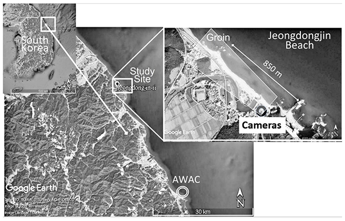
Figure 1Location of Jeongdongjin Beach in Gangwon-do on the east coast of South Korea © Google Earth.

Figure 2Beach erosion at Jeongdongjin Beach, South Korea caused by (a) low waves on 4 December 2015 and (b) high waves on 10 February 2016.
On the east coast of Korea (Fig. 1), low waves from an east–northeasterly direction prevail in summer and high waves from the northeast dominate in winter. This causes seasonal change in shoreline orientation (Kim and Lee, 2015) as well as localized beach erosion up to 30 m on the downdrift side of some natural groins due to high waves in the winter months. For example, severe erosion with a maximum retreat of about 40 m was once observed (Fig. 2b) during February to March in 2016 on the updrift side of Jeongdongjin Beach (37∘41′37′′ N, 129∘02′26′′ E; Fig. 1) in Gangwon-do Province, where oblique high waves in winter encountered a cluster of natural pillar rocks protruding about 80 m into the open sea. Rail-bike (pedal-powered rail cycles) tracks and the inner wall of Hourglass Park were damaged (Fig. 3).
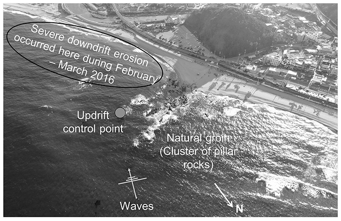
Figure 3Location of pillar rocks seaward of Jeongdongjin Beach, where downdrift erosion had occurred.
Beach erosion on the downdrift side of groins and its negative impact have been well studied theoretically or in prototype (Lehnfelt and Svendsen, 1958; Bakker, 1968, Bakker et al., 1970; Price and Tomlinson, 1970; Magoon and Edge, 1978; Headland et al., 2000; USACE, 2002). To investigate the effect of groins on beach erosion, Badiei et al. (1994) conducted laboratory experiments to reproduce the shoreline planform and topographic changes, while Wang and Kraus (2004) performed tests on erosion without longshore sediment transport (LST). A numerical approach has also been used. For example, Pelnard-Considèere (1956) proposed a one-line model that can simulate the temporal changes in the shoreline associated with groins. The applicability of this model has been verified in various situations by applying the concept of longshore diffusivity (e.g., Le Méhauté and Soldate, 1979; Walton and Chiu, 1979; Larson et al., 1987). Among them, Ozasa and Brampton (1980) developed a beach topography change model that can simulate a crenulate shape due to wave diffraction. Hanson and Kraus (1989) produced the generalized shoreline change model for calculating long-term shoreline changes, while Leont'yev (1997) proposed a short-term shoreline change model. However, most of these have not specifically reported the magnitude of downdrift erosion caused by oblique waves to a groin.
The long-term stability of the shoreline depends on the balance between the LST and sediment characteristics at wave breaking (Longuet-Higgins, 1970a, b; Komar and Inman, 1970; USACE, 1984; Kamphuis, 1991; Bayram et al., 2007). Because a new shoreline planform induced by downdrift erosion may reach a stable condition, it is imperative to assess its equilibrium status using an appropriate model, empirical and/or numerical (Balaji et al., 2017). Among the empirical models available for embayed beaches, which include a logarithmic spiral (Krumbein, 1944; Yasso, 1965), a parabolic bay shape model (PBSE; Hsu and Evans, 1989) and a hyperbolic tangent model (Moreno and Kraus, 1999), only the parabolic model is derived for the static equilibrium planform (SEP). When an SEP is reached, LST is not required to maintain the shoreline stability because waves would break simultaneously along the bay periphery (Hsu et al., 2000). Nowadays, together with the equilibrium beach profile, the concept of the equilibrium beach that incorporates the parabolic model for the shoreline planform has been widely used in the engineering design for beach nourishment projects (González et al., 2010) and as a means for project planning (USACE, 2002). Recently, Lim et al. (2019) have also confirmed the validity of the parabolic model using wave data from the east coast of South Korea, to estimate the impact of engineering structures (e.g., jetties and groins). Moreover, Lim et al. (2021) have also demonstrated the effect of wave diffraction caused by coastal structures, supported by numerical models (e.g., Xbeach and Sbeach) that include waves, currents and topographic changes.
The aims of this paper are threefold: (1) to derive mathematical equations for calculating the position of the maximum indentation in the eroded beach, (2) to demonstrate the applicability of an analytical model derived from the parabolic model and (3) to apply the mathematical equation to downdrift erosion at Jeongdongjin in Korea. These equations are solved using the prevailing wave conditions and the LST in winter months at Jeongdongjin, which are obtained from analyzing NOAA's wave data. In this paper, a brief introduction is first given in Sect. 1, while Sect. 2 describes the analytical model using the parabolic model and the derivation of mathematical equations for the downdrift control point and the maximum indentation on the eroded beach. Analysis of NOAA's wave data over 40 years is presented in Sect. 3.1 which provides averaged wave heights and wave angles at breaking for solving the mathematical equations (Sect. 2.2 and 2.3) and the seasonal LST rate (Sect. 3.2) for the one-line shoreline change model outlined in Sect. 4. The analytical results for the maximum indentation point are then compared with the results of the numerical model and that from the shoreline video monitoring project at Jeongdongjin Beach (Sect. 4). Finally, discussions on the limitation of the proposed analytical model and the effect of sediment bypassing are given in Sect. 5. Concluding remarks are given in Sect. 6.
2.1 Parabolic bay shape model
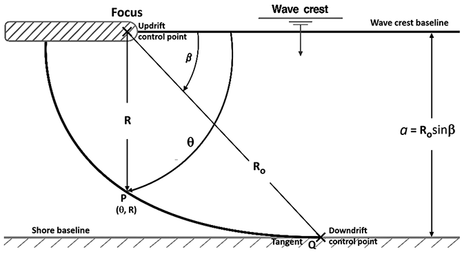
This empirical model is based on the parabolic bay shape equation (PBSE; Hsu and Evans, 1989) that defines the location of a point P(θ,R) on an embayed beach in static equilibrium (SEP) by
As shown in Fig. 4, R denotes the radial distance from the parabolic focus (i.e., updrift control point) to a point (P) on the equilibrium shoreline; a is the distance between the wave crest baseline at the focus, and the tangent passing through the downdrift control point (Q) is parallel to the wave crest baseline; β is the angle between the wave crest baseline and the line joining the focus and point Q; θ is between the wave crest baseline and the radius R. Coefficients C0, C1 and C2 are the values derived from the regression analysis of 27 SEPs in mixed cases of laboratory and prototype data (Hsu and Evans, 1989). At point Q, the boundary condition requires (unity) to ensure a common tangent at θ=β.
When the downdrift straight section of an embayment is long, Eq. (1b) can be approximated as
If waves break at an angle αb around the downdrift control point Q, then αb can be expressed by Eq. (3) from the approximation of Eq. (2). In the absence of β in Eq. (3), θ can be solely determined from wave angle αb at wave breaking or vice versa:
The relationship between θ and αb in Eq. (3) for an SEP can be readily calculated and expressed explicitly using a figure or table. For example, the three key values of αb (=10, 20 and 30∘) correspond to θ of 52.5, 71.2 and 86.5∘, respectively.
2.1.1 Downdrift control point
Consider a simple littoral cell without sediment supply from the updrift side, in which shoreline and depth contour are initially straight and parallel, that is subjected to oblique wave action and the LST is blocked within two groins: one short unit on the left-hand side and another long unit on the right-hand side (Fig. 5). Initially, beach erosion is minor, when the downdrift control point (or transition point A) reaches one-sixth of the length between the groins, without wave diffraction (top panel in Fig. 5). Under a longer duration of wave action, beach erosion on the downdrift side of a short groin increases and the control point A could be extended downward reaching one-third of the length (B) between the groins. A crenulate bay shape is not developed, due to no wave diffraction. As wave action continues, the length of beach erosion expands, with control point C reaching one half of the beach length (lower panel in Fig. 5). In this figure, parameters , and denote the time when the control point reaches one-sixth, one-third and half of the beach length L between the groins, respectively. At , the planform will remain in equilibrium.
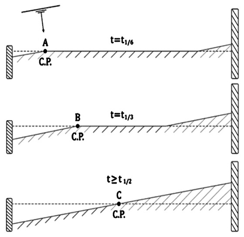
Figure 5Temporal variations in downdrift control point due to oblique waves within a littoral cell.
In the case of a short groin without bay shape formation, the position of the control point xc, measured from the groin on the left-hand side, can be expressed as a function of the elapsed time t and the LST rate Ql (see Sect. 3.2). From the relationship of planar sediment area and beach geometry,
this gives
where the LST rate Ql (unit: [m3]) is given by ), in which αb is the wave angle at breaking, qb has the unit of m2 and η () has the unit of [m]. Equation (4) indicates that the position of the control point is a function of LST rate, wave angle αb at breaking and time (), from which the time elapsed for the control point to reach a distance of xc can be rearranged as
where τ is defined as . When the eroded beach reaches SEP, , where L=850 m is the length of the shoreline between two groins (Fig. 1), and the time elapsed can be given by
Equation (6) implies that the time required to reach equilibrium increases as the LST decreases but as beach length and wave obliquity increase. This approach can also be applied to a single littoral cell system affected by wave diffraction around a moderate or long groin with protruding length yg, which is located at using the parallel shoreline assumption (see definition sketch of parabolic model in Fig. 4) of Hsu and Evans (1989). Hence, the shoreline advance width () of the parallel shoreline is expressed as
where β is assumed to converge to zero, C1 is unity, and C0 and C2 are zero.
2.1.2 Maximum indentation point
In Fig. 6, the cross mark “×” indicates the maximum indentation position on each of the beach erosion shapes at different time steps. Here, the shoreline orientation at the downdrift end is assumed to be the same as the wave breaking angle (αb) for applying the parabolic model based on the downdrift control point (A, B and C, respectively, as in Fig. 6) at each time step. An example is illustrated in Fig. 7.
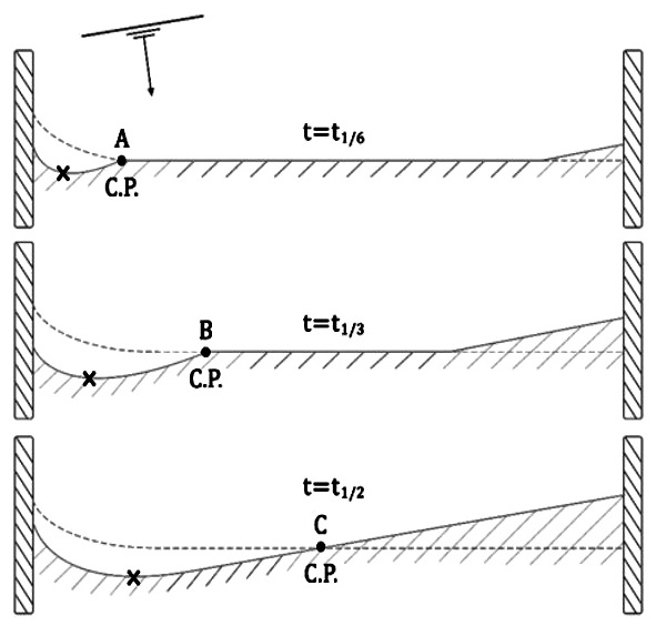
Figure 6Temporal change in the downdrift control point (C. P.) for applying the parabolic model including the effect of wave diffraction due to oblique waves within a littoral cell, also showing maximum indentation (×) at each time step.
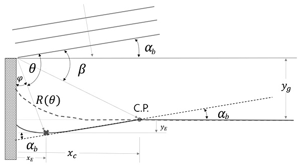
Figure 7Application of the parabolic model based on the estimation of αb and downdrift control point (C. P.) and wave diffraction on the downdrift side of a groin.
The location of the maximum indentation point (xE, yE), shown in Fig. 7, can be determined using the PBSE approximation given by
where angle θ is for locating the maximum indentation given by Eq. (3) from the wave direction αb at breaking. In addition, xE is the distance measured from the groin in the direction of the initial (mean) shoreline, and R(θ) is a time-variant function of xc, which can be obtained by Eq. (9) using the approximation of the parabolic model in Eq. (2):
Applying Eqs. (9) to (8a, b) results in an alternative expression for xE and yE:
where . Consequently, a linear relationship for xE and yE can be established:
Moreover, Eqs. (10a, b) and (11) can be non-dimensionalized using yg, giving
where . Figure 8 shows the locations of and as a function of dimensionless (0 to 4 with increments of 1.0) and different values of αb from 1 to 30∘. This figure indicates that the erosion width yE increases with the increase in several parameters (i.e., the protruding length of the groin yg, qb, t and αb).
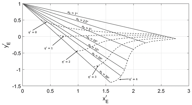
Figure 8Location of and for maximum indentation point, based on the dimensionless variable .
2.2 Longshore sediment transport equation
Komar and Inman (1970) conducted field experiments on longshore energy flux, Pl, and longshore sediment transport (LST) rate, Ql, expressing their relationship as
where ρ, ρs, p and g are the seawater density, sediment density, sediment porosity (typically about 0.3–0.4) and acceleration due to gravity, respectively. Il is the immersed weight of the sediment transport rate, and K is a dimensionless coefficient (e.g., Coastal Engineering Research Center – CERC – coefficient) dependent on seabed property and significant wave height, which can be taken as 0.39 (USACE, 1984) but was taken as 0.77 in Komar and Inman (1970). The alongshore component of the energy flux per unit length of beach Pl is defined by
where subscript “b” denotes the condition at wave breaking, (ECg)b is the wave energy flux at breaking, and αb is the breaking wave angle between the shoreline and wave crest line. Equations (14) and (15) can be combined and expressed as a function of wave height (Hb) and breaking wave direction (αb):
where the unit for Ql is [m3 s−1], has a value of 0.0847 for most types of sand, in which K=0.39, g=9.81 m s−2, spilling wave breaking index κ=0.78, and sediment specific gravity s=2.57 and porosity p=0.35 for most types of sand.
The LST rate in Eq. (16) can be expressed using deep-water wave data shown in Eq. (17), assuming that the isobath of the seabed is parallel to the straight shoreline, resulting in
where Col is a constant and Ho and To are the significant wave height and wave period in deep water, respectively. The wave direction in the deep-water αo is measured between the outward normal to the shoreline and wave orthogonal or from the true north θo, as shown in Fig. 9; thus , with a positive amount of sediment pointing south and a negative pointing north. Furthermore, Col is a factor that reflects the characteristics of the sediment and waves, including specific gravity, porosity, breaking index and wave angle, giving
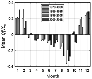
where Col=0.0719 approximately for most types of sand, assuming the effect of αb is negligible. The monthly distribution of is presented in Fig. 12.
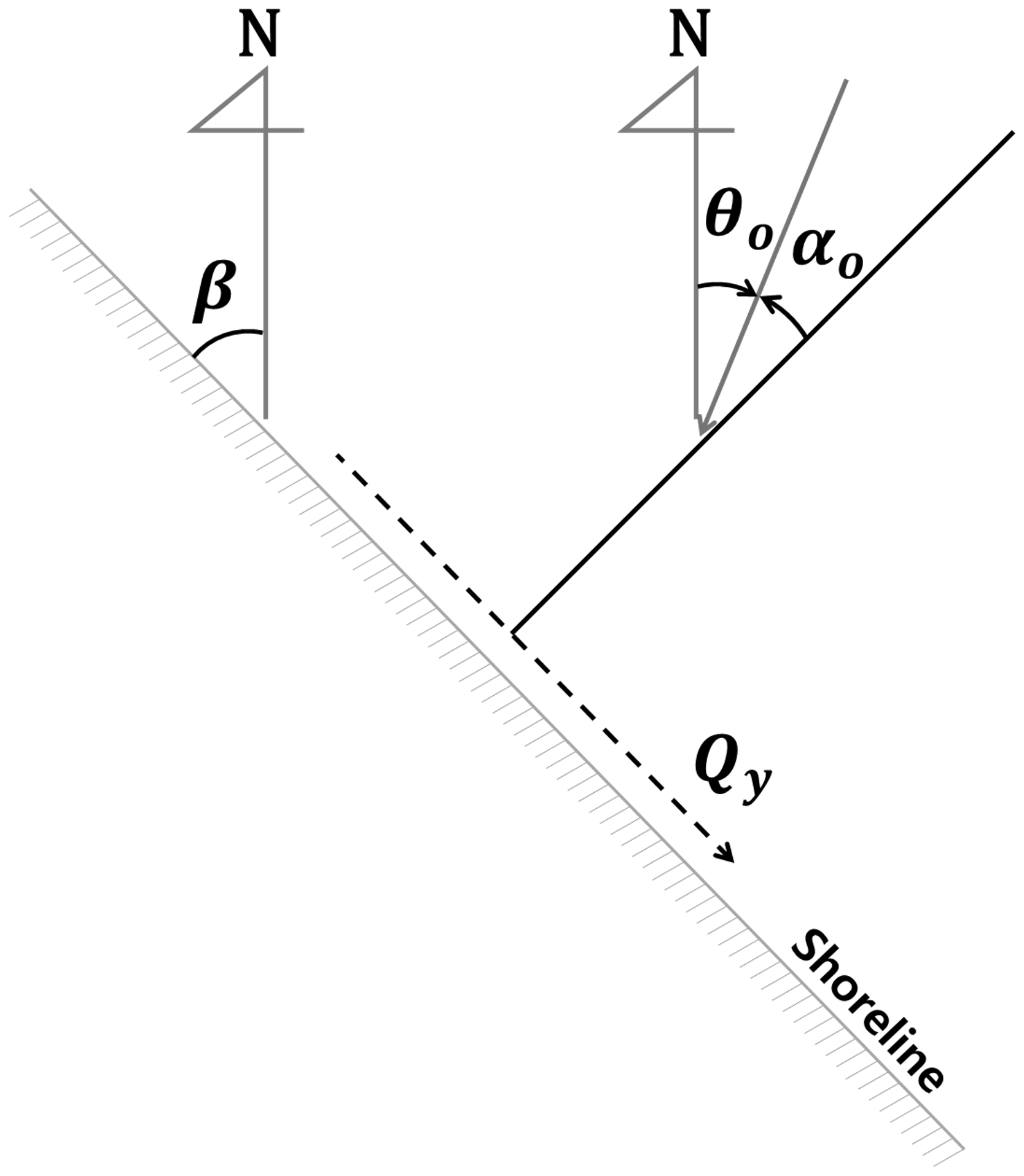
Figure 9Definition sketch showing deep-water wave angle αO and others for calculating LST rate in this study.
The long-term shoreline change is calculated using a one-line model (Pelnard-Considèere, 1956), by considering the difference in the LST along the coast within the active zone between the berm and the depth of closure:
where (x, y) are the Cartesian coordinates with the x axis positive pointing seaward, the y axis pointing alongshore and the origin being at the mean shoreline (MSL); hB and hC are the berm height and closure depth, respectively. Ql is the LST rate calculated by the CERC formula (USACE, 1984), and q represents the cross-shore sediment transport per unit width of the shoreline (Lee and Hsu, 2017). An alternative expression for the LST rate, similar to Eq. (17), is given by
where αm is the wave angle within the diffracted zone (Lim et al., 2021). However, nearshore currents within the diffraction zone are assumed to be in non-existent when SEP is reached for the eroded shoreline planform. In the numerical calculations, the quantity of the LST at each grid is calculated or assigned. For example, Ql=0 is used for the eroding shoreline along the boundary of the groin.
Jeongdongjin Beach (Fig. 1) in Gangwon-do, South Korea, is a littoral cell about 850 m long bounded between two groins – a cluster of pillar rocks behaving like a natural groin in the north end and a land-based artificial structure in the south. The wave data and sediment LST rate required for calculating the spatial and temporal location of the downdrift control point (i.e., xc in Eq. 4) and maximum indentation point (i.e., xE and yE in Eq. 10) can be obtained from analyzing NOAA's wave data.
3.1 NOAA wave data (1979–2018)
The European Center for Medium-Range Weather Forecasts and the National Centers for Environmental Prediction (NCEP) under the National Oceanic and Atmospheric Administration (NOAA) in the United States have provided long-term wave hindcast data since January 1979. Since 2004, NOAA has also operated the Climate Forecast System Reanalysis and Reforecast (CFSRR) activity, which analyzes sea climate using observation data that span more than 60 years. Saha et al. (2010, 2014) have verified the applicability of NOAA data by assimilating and verifying CFSRR observation data.
For the wave conditions in the open sea applicable to Jeongdongjin Beach, NOAA wave data between 1979 and 2018 are available for a nearby location (38.0∘ N, 129.5∘ E). The wave data are analyzed and the results used to calculate the change in the eroding shoreline curve on the downdrift side of the natural rocky groin caused by the oblique high waves in the winter. First, the monthly root-mean-square (rms) wave height () is calculated using Eq. (21):
where N is the total number of wave data. In addition, the mean wave period and direction, and , can also be calculated from the wave data. Figure 10 depicts the monthly variations in the rms wave height, period and direction of the significant waves, averaged over every 10-year interval between1979 and 2018. As shown in this figure, the NE waves in winter (December–February) arrive from 10∘ E approximately, the ENE waves in summer (June–August) approach the study area from 70∘ E, and the local shoreline aligns in a NW–SE direction (about 133∘ E).
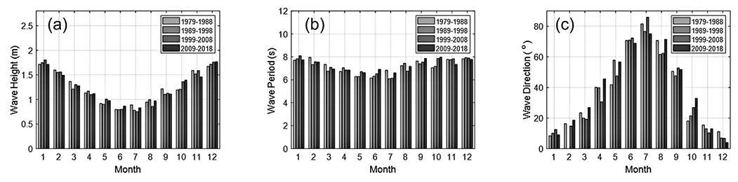
Figure 10Averaged monthly wave conditions for the study area: (a) wave height, (b) wave period and (c) offshore wave direction.
Nearshore wave data were also collected by an acoustic wave and current meter (AWAC) (see Fig. 1 for location) to the south of Jeongdongjin Beach at a depth of 32.4 m. From the data recorded over 3 years (27 September 2013 to 21 November 2016), the distribution of the annual mean wave direction is plotted (Fig. 11). The results reveal the prevailing nearshore wave direction was mostly within −15 to +10∘ from the normal to the local shoreline. However, positive values are only responsible for downdrift erosion of the natural groin at the updrift of Jeongdongjin Beach.
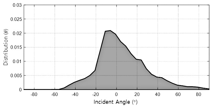
Figure 11Distribution of the mean wave direction collected by an AWAC meter to the south of Jeongdongjin Beach.
By plotting the monthly wave factor for the LST rate in terms of , using NOAA wave data, the results in Fig. 12 reveal a strong seasonally dependent trend in the direction of the LST, highlighting southward transport in winter months (November to February) and northward transport in summer (July to September). Thus, downdrift beach erosion can be expected to reach a maximum around February at the end of winter. However, if the seasonal LST bypasses the beach without being intercepted by the rocky pillars (Fig. 3) at different water levels and wave conditions, only weak to moderate downdrift erosion could result.
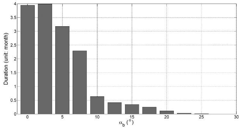
Assuming the seabed contours are straight and parallel, then the wave height and wave angle at the breaker are estimated from satisfying linear wave shoaling and refraction relationship () and spilling wave breaking criteria (hb=1.28Hb) simultaneously (Reeve et al., 2012) from the waves offshore collected in NOAA's wave data. From the results, the monthly average of as a function of the oblique wave direction αb in 2.5∘ intervals is graphed (Fig. 13) for waves in winter months (November–February). The wave angle is evaluated based on 38∘ E as αb=0, and the wave height and angle at breaking are calculated by 38∘ E ± 50∘ in deep water. The values of were large within −7.5 to +12.5∘, which implies that high waves in winter which may cause severe beach erosion could arrive from the sector within 38–2.5∘ E to 38+7.5∘ E.

Figure 13Monthly average of per 2.5∘ interval of oblique wave angle αb, obtained from NOAA wave data during winter months.
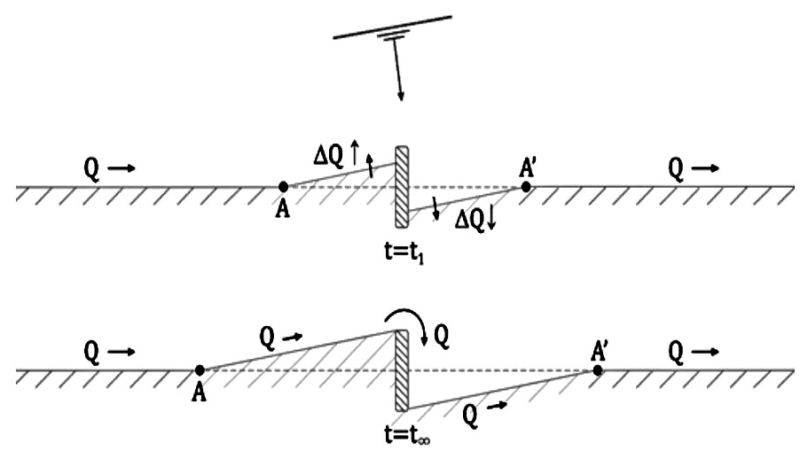
If an amount of LST (ΔQ) to a beach is accreted on the updrift side of a groin on a straight shoreline (Fig. 14), the shoreline retreats on the downdrift side. Once sediment bypasses the tip of the groin, a long-term shoreline equilibrium may be reached on both sides of the groin. However, during this process of bypassing, the location of A and A' may fluctuate, with the former gradually advancing updrift while the latter slowly shift downdrift.
3.2 Shoreline video monitoring program
Shoreline monitoring in South Korea has been conducted since 2003, as part of the national Coastal Erosion Survey Project, aiming to promote efficient coastal maintenance in the country via proactive responses based on scientific data collection and analysis. At Jeongdongjin, the video monitoring program commenced in February 2014, with the installation of four cameras to cover the shoreline of the beach (Fig. 1).
In this study, the variation in shoreline positions was derived from the time-averaged video images by the geometric transformation equation (Lippmann and Holman, 1989), which transforms the image coordinates to ground coordinates. The video images were taken twice a day from 6 to 30 December in 2015, while the routine one per day operation was continued in the following January and February in 2016 (shown in Fig. 17). However, it should be noted that the location of the critical points on these images might not include that of the instantaneous maximum indentation. Therefore, the actual extent of shoreline retreat may be larger than that presented.
In this section, the performance of the analytical model is verified by comparing not only the numerical model but also the shoreline data. Figure 15 compares the temporal variation in the results for analytical and numerical (Lim et al., 2021) results of xE and yE at the maximum indentation for τ (; unit of meters and hours) for three different values of αb (10, 15 and 20∘) at Jeongdongjin Beach with a natural rocky groin about 80 m long. In the numerical results, the value of yE (negative) increases (erosion) with time as αb increases, whilst that of xE decreases (closer to the boundary from the groin). A similar trend can be found in the analytical results. Moreover, the discrepancies between the numerical and analytical results increase as αb increases.
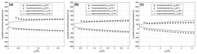
Figure 15Comparison between analytical and numerical results for breaking wave direction αb of (a) 10∘, (b) 15∘ and (c) 20∘ for Jeongdongjin Beach.
Table 1Comparison between the control point locations obtained from NOAA wave data and from Eq. (22).
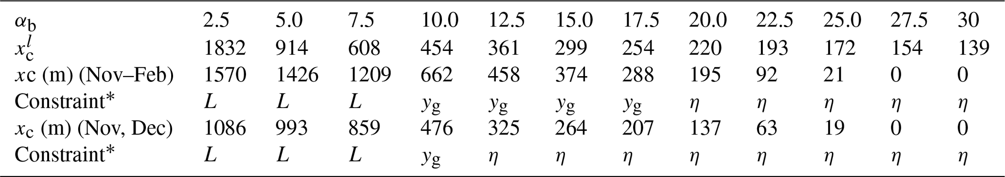
* Parameters in the rows labeled “Constraint*”: L for constraint by beach length, η by longshore drift length () and yg by protruding length of groin.
In addition, the planform of the eroded beach can be simulated using a numerical model. First, the results of the numerical model for a series of duration from 6 h to 4 weeks can be demonstrated, using αb=10∘ (Fig. 13), which is indicated in Fig. 16, using the prototype data for Jeongdongjin Beach (i.e., natural groin with protruding length yg=80 m, beach length L=850 m, winter high waves of 2.11 m and LST coefficient C=0.0847 in Eq. 16). In this figure, the shoreline near the groin advances seaward within the first 6 h, similar to the trend in Fig. 15a, prior to being eroded (landward) thereafter. For αb=10∘, and the maximum erosion length xc=425 m (i.e., not exceeding ), Eq. (16) gives m, which is equivalent to the result of “1 week after” in the numerical model. In addition, the analytical method is also applied for other wave angles at breaking (αb) at 2∘ intervals, and the results are collectively marked as “theoretical results” in Fig. 17.
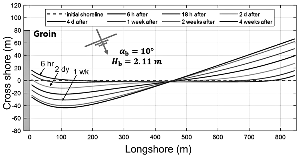
Figure 16Results of the numerical model, showing spatial and temporal variation in the eroding beach planform for αb=10∘.
The results of the analytical method predict the eroding shoreline planform and the maximum indentation point using the parabolic model with monthly averaged wave conditions from NOAA wave data, whereas the results of the video monitoring program reveal the hourly/daily record from the shoreline images corresponding to the instantaneously changing wave conditions. To compare the results coming from these two different sources, the maximum indentation points occurring on the day of video recording are selected. Despite the difference in timescale, Fig. 17 indicates that the results of the analytical prediction are in fair agreement with the video monitoring data. At the duration of 0.6 months (18 d) for waves with αb=10∘ (Fig. 18) obtained from NOAA wave data, the numerical model predicts that the maximum indentation may reach 40 m for wave actions lasting about 2 weeks (Fig. 16), which also agrees reasonably well with the shoreline video monitoring results (Fig. 17).
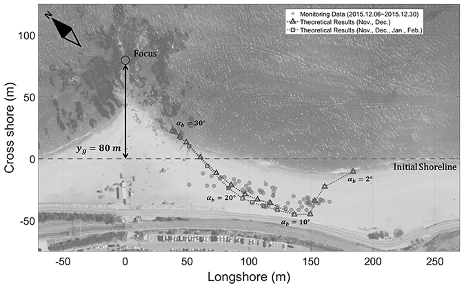
Figure 17Comparison between video monitoring data and analytical solution © National Geographic Information Institute (NGII).
This paper deals with downdrift erosion – a shoreline retreat hotspot on the downdrift side of a natural rocky groin that interrupts the longshore transport during high waves in winter. A prediction for the resultant embayed geometry is developed by deriving mathematical equations from the parabolic bay shape model (Hsu and Evans, 1989). The validity of this analytical model is confirmed for Jeongdongjin Beach on the northeast coast of South Korea by using video monitoring data and one-line numerical models. When applying this method to other beaches, however, consideration/modification must be taken for locating the downdrift control point because Jeongdongjin Beach is a littoral cell with 850 m length (Fig. 1), while the others may not be the same coastal environments. Nevertheless, this robust method can be used as a suitable first approximation and will be useful for practical engineers since the approach can be easily applied if long-term wave data (e.g., NOAA wave data) or shoreline video monitoring results are available.
The method presented in this paper excludes sediment bypassing through the groin on the updrift side as well as the shoreline retreat due to cross-sediment movement. Therefore, the analytical results for the maximum indentation from Eq. (10a, b) with the LST rate might be underestimated. To include sediment bypassing, the alongshore distance of the downdrift control point (at xc in Fig. 7) will be limited with the breaking wave angle αb in relation to the protruding length of the groin (Figs. 1 and 17), considering the following relationship:
where superscript “l” denotes the limiting value. Here, variables xc and , obtained from Eqs. (10a, b) and (23), respectively, are compared in Table 1. If xc obtained for each αb is greater than for a given yg, then xc should be replaced by because bypassing might not occur for αb between 10 and 17.5∘. As shown in Fig. 17, the monitoring data in December 2015 support the analytical solution that uses αb=10∘ for calculating the xc. In Table 1, η () indicates that there is no effect of protruding length yg or beach length L (=850 m) because either the LST rate is small or the wave duration is too short. However, the erosion width may be reduced as bypassing occurs when the protruding length is short. Thus, the limit in xc relative to L is expected to be within one half of the beach length ( m, where L=850 m), which is within the range of beach length covered by the video monitoring equipment.
The present method can be used to estimate the eroding shoreline planform for a beach nourishment project, especially by comparing the position of the maximum indentation. For example, to mitigate the extent of downdrift erosion caused by winter high waves, engineering options may be considered either by (1) artificially nourishing the beach to advance the shoreline (Fig. 19) or (2) placing a short groin to promote sediment accretion within the potentially eroding section (Fig. 20). Figure 19 compares the reduction in potential beach erosion and its maximum depth yE for uniformly nourishing the beach by 10 and 20 m, respectively, which gives yE of −38 and −30 m, respectively, compared with the potential beach erosion without artificial nourishment ( m) under the same wave condition.
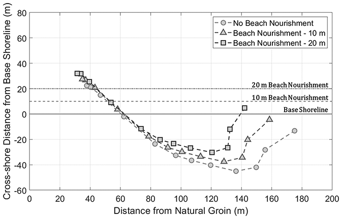
Figure 19Change in maximum erosion width and indentation induced by beach nourishment of two different widths.

Figure 20 illustrates the temporal shoreline change by placing a short groin at point G where it becomes a new downdrift control point for the potential eroded beach curve. Therefore, the dimension of a potentially eroding beach on the downdrift side of the natural groin can be reduced by sediment accretion fronting the short groin. For example, to limit the maximum erosion of yE within 20 m for αb=10∘ during winter high waves, a groin may be installed at 327 m from the groin, for which the location can be estimated by Eq. (10b), giving
in which yg=80 m and φ=47.5∘ for αb=10∘.
Downdrift erosion – a phenomenon of localized erosion at the unprotected downdrift end of seawalls or groins – is common, but it is rarely taught in the classrooms nor well documented in the literature and coastal engineering journals, leaving a challenging problem for the consulting engineers and coastal managers to deal with (e.g., Headland et al., 2000). During the winter months on the east coast of South Korea, oblique high waves have often generated severe erosion at the downdrift stretch of a groin, natural or artificial. For example, beach erosion on the downdrift side of a cluster of natural pillar rocks at Jeongdongjin had occurred continuously for more than 2 consecutive months (February–March) in 2016. Video footage revealed that, during this period, the eroded beach remained in a distinctive crenulate shape with a maximum indentation of about 40 m over some 300 m. Despite the beach gradually having recovered in the following months (May–June) in calm weather, the erosive scenario had caused disastrous effects not only for the beach environment but also the livelihood of the locals.
The purpose of this study is to introduce an analytical model, simple yet useful, that can help predict the size and shape of the eroded beach of downdrift side to benefit local coastal managers in maintaining the beaches. By the input of wave conditions (heights and wave angle at breaking) and updrift control point (wave diffraction point) to the mathematical equations derived from the parabolic model for bay beaches in static equilibrium, the maximum indentation and crenulate bay shape can be predicted. This method is robust and cost effective, compared to the time-consuming and costly physical experiments and the complex numerical models.
This study's wave data are available in the WAVEWATCH III® Hindcast and Reanalysis Archives at the National Weather Service, National Oceanic and Atmospheric Administration (https://polar.ncep.noaa.gov/waves/hindcasts; NOAA, 2022). Other data sets used in this work can be requested by email from the author (art3440@naver.com).
CL and JLL conceived the idea. CL and SH participated in the field data collection. CL and JLL participated in the analysis of the data. CL and JLL participated in visualization of the figures. All authors contributed to the writing of the final draft.
The contact author has declared that neither they nor their co-authors have any competing interests.
Publisher's note: Copernicus Publications remains neutral with regard to jurisdictional claims in published maps and institutional affiliations.
This research was part of the “Practical Technologies for Coastal Erosion Control and Countermeasure” project supported by the Ministry of Oceans and Fisheries, South Korea (grant no. 20180404).
This paper was edited by Orencio Duran Vinent and reviewed by two anonymous referees.
Badiei, P., Kamphuis, J. W. and Hamilton, D. G.: Physical experiments on the effects of groins on shore morphology, in: Proceedings of the Coastal Engineering Conference, 2, 1782–1796, https://doi.org/10.1061/9780784400890.129, 1994.
Bakker, W. T.: The dynamics of a coast with a groin system, in: Proc. 11th Inter. Conf. Coastal Eng. ASCE, 492–517, https://doi.org/10.9753/icce.v11.31, 1968.
Bakker, W. T., Klein Breteler, E. H. J., and Roos, A.: The dynamics of a coast with a groin system, in: Proc. 12th Inter. Conf. Coastal Eng. ASCE, 64, 1001–1020, https://doi.org/10.9753/icce.v12.64, 1970.
Balaji, R., Kumar, S. S., and Misra, A.: Understanding the effects of seawall construction using a combination of analytical modelling and remote sensing techniques: Case study of Fansa, Gujarat, India, J. Ocean Clim. Syst., 8, 153–160, 2017.
Bayram, A., Larson, M., and Hanson, H.: A new formula for the total longshore sediment transport rate, Coast. Eng., 54, 700–710, https://doi.org/10.1016/j.coastaleng.2007.04.001, 2007.
González, M., Medina, R., and Losada, M.: On the design of beach nourishment projects using static equilibrium concepts: Application to the Spanish coast, Coast. Eng., 57, 227–240, https://doi.org/10.1016/j.coastaleng.2009.10.009, 2010.
Hanson, H. and Kraus, N.C.: GENESIS: Generalized Model for Simulating Shoreline Change, Report 1: References manual and users guide, Tech. Report CERC-89-19, US Army Corps of Engineers, Coastal Engineering Research Center, USA, https://doi.org/10.5962/bhl.title.48202, 1989.
Headland, J., Smith, W. G., Kotulak, P., and Alfageme, S.: Coastal protection methods, in: Handbook of Coastal Engineering, chap. 8, edited by: Herbich, J. B., McGraw Hill, NY, 8.1–8.66, ISBN 978-0071344029, 2000.
Hsu, J. R. C. and Evans, C.: Parabolic bay shapes and applications, Proc. Inst. Civ. Eng.s, 87, 557–570, https://doi.org/10.1680/iicep.1989.3778, 1989.
Hsu, J. R. C., Uda, T., and Silvester, R.: Shoreline protection methods – Japanese experience, in: Handbook of Coastal Engineering, edited by: Herbich, J. B., McGraw-Hill, New York, 9.1–9.77, ISBN 0-07-134402-0, 2000.
Kamphuis, J. W.: Alongshore Sediment Transport Rate, J. Waterw. Port Coast. Ocean Eng., 117, 624–641, https://doi.org/10.1061/(asce)0733-950x(1991)117:6(624), 1991.
Kim, D. S. and Lee, G.-R.: Seasonal Changes of Shorelines and Beaches on East Sea Coast, South Korea, J. Korean Geogr. Soc., 50, 147–164, 2015.
Komar, P. D. and Inman. D. L.: Longshore sand transport on beaches, J. Geophys. Res., 75, 5914–5927, https://doi.org/10.1029/jc075i030p05914, 1970.
Kraus, N. C. and McDougal, W. G.: The effects of seawalls on beaches, Part 1: An updated literature review, J. Coast. Res., 12, 691–701, 1996.
Krumbein, W. C.: Shore Processes and Beach Characteristics, in: Technical Memorandum, vol. 3, Beach Erosion Board, US Army Corps of Engineers, p. 47, https://hdl.handle.net/11681/3390 (last access: 4 March 2022), 1944.
Larson, M., Hanson, H., and Kraus, N. C.: Analytical solutions of the 1-line model of shoreline change, Tech. Rep. – US Army Coast. Eng. Res. Cent., 87–15, https://doi.org/10.5962/bhl.title.48288, 1987.
Lee, J. L. and Hsu, J. R. C.: Numerical simulation of dynamic shoreline changes behind a detached breakwater by using an equilibrium formula, in: Proceedings of the International Conference on Offshore Mechanics and Arctic Engineering – OMAE, 7A, V07AT06A036, https://doi.org/10.1115/OMAE2017-62622, 2017.
Lehnfelt, A. and Svendsen, S. V.: Thyboroen channel – difficult coastal protection problem in Denmark, Ingenioeren, 2, 66–74, 1958.
Le Méhauté, B. and Soldate, M.: Mathematical modeling of shoreline evolution, in: Proceedings of the Coastal Engineering Conference, 2 pp., https://doi.org/10.9753/icce.v16.67, 1979.
Leont'yev, I. O.: Short-term shoreline changes due to cross-shore structures: A one-line numerical model, Coast. Eng., 31, 59–75, https://doi.org/10.1016/S0378-3839(96)00052-X, 1997.
Lim, C., Lee, J., and Lee, J. L.: Simulation of bay-shaped shorelines after the construction of large-scale structures by using a parabolic bay shape equation, J. Mar. Sci. Eng., 9, 43, https://doi.org/10.3390/jmse9010043, 2021.
Lim, C. B., Lee, J. L., and Kim, I. H.: Performance test of parabolic equilibrium shoreline formula by using wave data observed in east sea of korea, J. Coast. Res., 91, 101–105, https://doi.org/10.2112/SI91-021.1, 2019.
Lippmann, T. C. and Holman, R. A.: Quantification of sand bar morphology: a video technique based on wave dissipation, J. Geophys. Res., 94, 995–1011, https://doi.org/10.1029/JC094iC01p00995, 1989.
Longuet-Higgins, M. S.: Longshore currents generated by obliquely incident sea waves, 1., J. Geophys. Res., 75, 6778–6789, 1970a.
Longuet-Higgins, M. S.: Longshore currents generated by obliquely incident sea waves, 2., J. Geophys. Res., 75, 6790–6801, 1970b.
Magoon, O. T. and Edge, B. L.: Stabilization of shoreline by use of artificial headlands and enclosed beaches, in: Proc. Coastal Zone'78, ASCE, 14–16 March 1978, v. 2, 1367–1370, 1978.
Moreno, L. J. and Kraus, N. C.: Equilibrium Shape of Headland-Bay Beaches for Engineering Design, in: Proceedings of the Coastal Sediments'99, 21–23 June 1999, 860 pp., 1999.
NOAA – National Oceanic and Atmospheric Administration: WAVEWATCH III® Hindcast and Reanalysis Archives, NOAA [data set], https://polar.ncep.noaa.gov/waves/hindcasts, last access: 3 March 2022.
Ozasa, H. and Brampton, A. H.: Mathematical modelling of beaches backed by seawalls, Coast. Eng., 4, 47–63, https://doi.org/10.1016/0378-3839(80)90005-8, 1980.
Pelnard-Considèere, R.: Essai de theorie de l'evolution des formes de rivage en plages de sable et de galets, Journées de L'hydraulique, 4, 289–298, 1956.
Price, W. A. and Tomlinson, K. W.: The effect of groynes on eroded beaches, in: chap. 67, Proc. 12th Inter. Conf. Coastal Eng., ASCE, 29 January 1970, 1053–1058, 1970.
Reeve, D., Chadwick, A., and Fleming, C.: Coastal Engineering: Processes, Theory and Design Practice, 2nd Edn., Spon Press, Taylors & Francis, London, 514 pp., ISBN 9781138060432, 2012.
Saha, S., Moorthi, S., Pan, H. L., Wu, X., Wang, J., Nadiga, S., Tripp, P., Kistler, R., Woollen, J., Behringer, D., Liu, H., Stokes, D., Grumbine, R., Gayno, G., Wang, J., Hou, Y. T., Chuang, H. Y., Juang, H. M. H., Sela, J., Iredell, M., Treadon, R., Kleist, D., Van Delst, P., Keyser, D., Derber, J., Ek, M., Meng, J., Wei, H., Yang, R., Lord, S., Van Den Dool, H., Kumar, A., Wang, W., Long, C., Chelliah, M., Xue, Y., Huang, B., Schemm, J. K., Ebisuzaki, W., Lin, R., Xie, P., Chen, M., Zhou, S., Higgins, W., Zou, C. Z., Liu, Q., Chen, Y., Han, Y., Cucurull, L., Reynolds, R. W., Rutledge, G. and Goldberg, M.: The NCEP climate forecast system reanalysis, B. Am. Meteorol. Soc., 91, 1015–1058, https://doi.org/10.1175/2010BAMS3001.1, 2010.
Saha, S., Moorthi, S., Wu, X., Wang, J., Nadiga, S., Tripp, P., Behringer, D., Hou, Y. T., Chuang, H. Y., Iredell, M., Ek, M., Meng, J., Yang, R., Mendez, M. P., Van Den Dool, H., Zhang, Q., Wang, W., Chen, M., and Becker, E.: The NCEP climate forecast system version 2, J. Climate, 27, 2185–2208, https://doi.org/10.1175/JCLI-D-12-00823.1, 2014.
USACE – US Army Corps of Engineers: Shore protection manual. Department of the Army, US Corps of Engineers, Washington, DC, 20314, 1984.
USACE: Coastal Engineering Manual, US Army Corps of Engineers, Washington, DC, USAm, http://chl.erdc.usace.army.mil/chl.aspx?p_s&a_articles;104, last access: 30 April 2002.
Walton, T. L. and Chiu, T. Y.: A review of analytical techniques to solve the sand transport equation and some simplified solutions, in: Proceedings of the Coastal Structures'79, ASCE, 14–16 March 1979, 809–837, 1979.
Wang, P. and Kraus, N. C.: Movable-Bed Model Investigation of Groin Notching, J. Coast. Res., 33, 342–368, 2004.
Yasso, W. E.: Plan Geometry of Headland-Bay Beaches, J. Geol., 73, 702–714, https://doi.org/10.1086/627111, 1965.