the Creative Commons Attribution 4.0 License.
the Creative Commons Attribution 4.0 License.
 | 11 Mar 2022
The landslide velocity
Shiva P. Pudasaini
Michael Krautblatter
Proper knowledge of velocity is required in accurately determining the enormous destructive energy carried by a landslide. We present the first, simple and physics-based general analytical landslide velocity model that simultaneously incorporates the internal deformation (nonlinear advection) and externally applied forces, consisting of the net driving force and the viscous resistant. From the physical point of view, the model represents a novel class of nonlinear advective–dissipative system, where classical Voellmy and inviscid Burgers' equations are specifications of this general model. We show that the nonlinear advection and external forcing fundamentally regulate the state of motion and deformation, which substantially enhances our understanding of the velocity of a coherently deforming landslide. Since analytical solutions provide the fastest, most cost-effective, and best rigorous answer to the problem, we construct several new and general exact analytical solutions. These solutions cover the wider spectrum of landslide velocity and directly reduce to the mass point motion. New solutions bridge the existing gap between negligibly deforming and geometrically massively deforming landslides through their internal deformations. This provides a novel, rapid, and consistent method for efficient coupling of different types of mass transports. The mechanism of landslide advection, stretching, and approaching the steady state has been explained. We reveal the fact that shifting, uplifting, and stretching of the velocity field stem from the forcing and nonlinear advection. The intrinsic mechanism of our solution describes the fascinating breaking wave and emergence of landslide folding. This happens collectively as the solution system simultaneously introduces downslope propagation of the domain, velocity uplift, and nonlinear advection. We disclose the fact that the domain translation and stretching solely depend on the net driving force, and along with advection, the viscous drag fully controls the shock wave generation, wave breaking, folding, and also the velocity magnitude. This demonstrates that landslide dynamics are architectured by advection and reigned by the system forcing. The analytically obtained velocities are close to observed values in natural events. These solutions constitute a new foundation of landslide velocity in solving technical problems. This provides practitioners with key information for instantly and accurately estimating the impact force that is very important in delineating hazard zones and for the mitigation of landslide hazards.
- Article
(3758 KB) - Full-text XML
- BibTeX
- EndNote


There are three methods to investigate and solve a scientific problem: laboratory or field data, numerical simulations of governing complex physical–mathematical model equations, or exact analytical solutions of simplified model equations. This is also the case for mass movements including extremely rapid flow-type landslides such as debris avalanches (Pudasaini and Hutter, 2007). The dynamics of a landslide are primarily controlled by the flow velocity. Estimation of the flow velocity is key for assessment of landslide hazards, design of protective structures, mitigation measures, and land use planning (Tai et al., 2001; Pudasaini and Hutter, 2007; Johannesson et al., 2009; Christen et al., 2010; Dowling and Santi, 2014; Cui et al., 2015; Faug, 2015; Kattel et al., 2018). Thus, a proper understanding of landslide velocity is a crucial requirement for an appropriate modeling of landslide impact force because the associated hazard is directly and strongly related to the landslide velocity (Huggel et al., 2005; Evans et al., 2009; Dietrich and Krautblatter, 2019). However, the mechanical controls of the evolving velocity, run-out, and impact energy of the landslide have not yet been understood well.
Due to the complex terrain, infrequent occurrence, and very high time and cost demands of field measurements, the available data on landslide dynamics are insufficient. Proper understanding and interpretation of the data obtained from field measurements are often challenging because of the very limited nature of the material properties and the boundary conditions. Additionally, field data are often only available for single locations and determined as static data after events. Dynamic data are rare (de Haas et al., 2020). So, many of the low-resolution measurements are locally or discretely based on points in time and space (Berger et al., 2011; Schürch et al., 2011; McCoy et al., 2012; Theule et al., 2015; Dietrich and Krautblatter, 2019). Therefore, laboratory or field experiments (Iverson et al., 2011; de Haas and van Woerkom, 2016; Lu et al., 2016; Lanzoni et al., 2017; Li et al., 2017; Pilvar et al., 2019; Baselt et al., 2021) and theoretical modeling (Le and Pitman, 2009; Pudasaini, 2012; Pudasaini and Mergili, 2019) remain the major source of knowledge in landslide and debris flow dynamics. Recently, there has been a rapid increase in comprehensive numerical modeling for mass transports (McDougall and Hungr, 2005; Medina et al., 2008; Cascini et al., 2014; Frank et al., 2015; Iverson and Ouyang, 2015; Cuomo et al., 2016; Mergili et al., 2020a, b; Qiao et al., 2019; Liu et al., 2021). However, to a certain degree, numerical simulations are approximations of the physical–mathematical model equations. Their usefulness is often evaluated empirically (Mergili et al., 2020a, b). In contrast, exact analytical solutions (Faug et al., 2010; Pudasaini, 2011) can provide better insights into the complex flow behaviors, mainly the velocity. Moreover, analytical and exact solutions to nonlinear model equations are necessary to elevate the accuracy of numerical solution methods (Chalfen and Niemiec, 1986; Pudasaini, 2011, 2016; Pudasaini et al., 2018). For this reason, here, we are mainly concerned with presenting exact analytical solutions for the newly developed general landslide velocity equation.
Since Voellmy's pioneering work, several analytical models and their solutions have been presented in the literature for mass movements including extremely rapid flow-type landslide processes, avalanches, and debris flows (Voellmy, 1955; Salm, 1966; Perla et al., 1980; McClung, 1983). However, on the one hand, all of these solutions are effectively simplified to the mass point or center of mass motion. None of the existing analytical velocity models consider advection or internal deformation. On the other hand, the parameters involved in these models only represent restricted physics of the landslide material and motion. Nevertheless, a full analytical model that includes a wide range of essential physics of the mass movements incorporating important process of internal deformation and motion is still lacking. This is required for the more accurate description of landslide motion. Moreover, recently presented simple analytical solutions for mass transports considered debris avalanches (Pudasaini, 2011), two-phase flows (Ghosh Hajra et al., 2017, 2018), landslide mobility (Pudasaini and Miller, 2013; Parez and Aharonov, 2015), fluid flows in debris materials (Pudasaini, 2016), mud flow (Di Cristo et al., 2018), granular front down an incline (Saingier et al., 2016), granular monoclinal wave (Razis et al., 2018), and submarine debris flows (Rui and Yin, 2019). However, neither a more general landslide model as we have derived here nor the solution for such a model exists in the literature.
This paper presents a novel nonlinear advective–dissipative transport equation with a quadratic source term representing the system forcing, containing the physical and mechanical parameters as a function of the state variable (the velocity) and their exact analytical solutions describing the landslide motion. The new landslide velocity model and its analytical solutions are more general and constitute the full description for velocities with a wide range of applied forces and the internal deformation. Importantly, the newly developed landslide velocity model covers both the classical Voellmy and inviscid Burgers' equations as special cases; it unifies and extends them further, but it also describes fundamentally novel and broad physical phenomena.
It is a challenge to construct exact analytical solutions even for the simplified problems in mass transport (Pudasaini, 2011, 2016; Di Cristo et al., 2018; Pudasaini et al., 2018). In contrast to the existing models, such as Voellmy-type and Burgers-type, the great complexity in solving the new landslide velocity model analytically derives from the simultaneous presence of the internal deformation (nonlinear advection, inertia) and the quadratic source representing externally applied forces (in terms of velocity, including physical parameters). However, here, we construct various analytical and exact solutions to the new general landslide velocity model by applying different advanced mathematical techniques, including those presented by Nadjafikhah (2009) and Montecinos (2015). We reveal several major novel dynamical aspects associated with the general landslide velocity model and its solutions. We show that a number of important physical phenomena are captured by the new solutions. This includes landslide propagation and stretching, wave generation and breaking, and landslide folding. We also observe that different methods consistently produce similar analytical solutions. This highlights the intrinsic characteristics of the landslide motion described by our new model. As exact analytical solutions disclose many new and essential physics, the solutions derived in this paper may find applications in environmental, engineering, and industrial mass transport down slopes and channels.
2.1 Mass and momentum balance equations
A geometrically two-dimensional motion down a slope is considered. Let t be time, (x, z) be the coordinates, and (gx, gz) the gravity accelerations along and perpendicular to the slope, respectively. Let h and u be the flow depth and the mean flow velocity along the slope. Similarly, let γ, αs, and μ be the density ratio between the fluid and the particles (), volume fraction of the solid particles (coarse and fine solid particles), and the basal friction coefficient (μ=tan δ), where δ is the basal friction angle, in the mixture material. Furthermore, K is the Earth pressure coefficient as a function of internal and basal friction angles, and CDV is the viscous drag coefficient.
We start with the multi-phase mass flow model (Pudasaini and Mergili, 2019) and include viscous drag (Pudasaini and Fischer, 2020). For simplicity, we assume that the relative velocity between coarse and fine solid particles (us, ufs) and the fluid phase (uf) in the landslide (debris) material is negligible: that is, , and so is the viscous deformation of the fluid. This means, for simplicity, we are considering an effectively single-phase mixture flow. Then, by summing up the mass and momentum balance equations (Pudasaini and Mergili, 2019; Pudasaini and Fischer, 2020), we obtain a single mass and momentum balance equation describing the motion of a landslide as
where emerges from the hydraulic pressure gradient associated with possible interstitial fluids in the landslide. Moreover, the term containing K on the left-hand side and the other terms on the right-hand side in the momentum equation (Eq. 2) represent all the involved forces. The first term in the square brackets on the left-hand side of Eq. (2) describes the advection, while the second term (in the square brackets) describes the extent of the local deformation that stems from the hydraulic pressure gradient of the free surface of the landslide. The first, second, third, and fourth terms on the right-hand side of Eq. (2) are the gravitational acceleration, effective Coulomb friction (which includes lubrication (1−γ), liquefaction (αs)) (because if there is no solid or a substantially low amount of solid, the mass is fully liquefied, e.g., lahar flows), the term associated with buoyancy and the fluid-related hydraulic pressure gradient, and the viscous drag, respectively. Note that the term with 1−γ or γ originates from the buoyancy effect. By setting γ=0 and αs=1, we obtain a dry landslide, grain flow, or an avalanche motion. For this choice, the third term on the right-hand side vanishes. However, we keep γ and αs to also include possible fluid effects in the landslide (mixture).
2.2 The landslide velocity equation
The momentum balance equation (Eq. 2) can be rewritten as
Note that for K=1 (which mostly prevails for extensional flows; Pudasaini and Hutter, 2007), the third term on the right-hand side associated with simplifies drastically because becomes unity. So, the isotropic assumption (i.e., K=1) loses some important information about the solid content and the buoyancy effect in the mixture. Employing the mass balance equation (Eq. 1), the momentum balance equation (Eq. 3) can be rewritten as
The gradient might be approximated, say as hg, and still include its effect as a parameter that may be estimated. Here, we are mainly interested in developing a simple but more general landslide velocity model than the existing ones that can be solved analytically and highlight its essence to enhance our understanding of landslide dynamics.
Now, with the notation (this includes the forces gravity, friction, lubrication, and liquefaction as well as the surface gradient) and β:=CDV (the viscous drag coefficient), Eq. (4) becomes a simple model equation:
where α and β constitute the net driving and the resisting forces in the system. We call Eq. (5) the landslide velocity equation.
2.3 A novel physical–mathematical system
Equation (5) constitutes a novel class of nonlinear advective–dissipative system and involves dynamic interactions between the nonlinear advective (or inertial) term and the external forcing (source) term α−βu2. However, in contrast to the viscous Burgers' equation wherein the dissipation is associated with the (viscous) diffusion, here, dissipation stems from the viscous drag, −βu2. In form, Eq. (5) is similar to the classical shallow-water equation. However, from the mechanics and the material composition, it is much wider as such a model does not exist in the literature. From the physical and mathematical point of view, there are two crucial novel aspects associated with the model (Eq. 5). First, it explains the dynamics of a deforming landslide and thus extends the classical Voellmy model (Voellmy, 1955; Salm, 1966; McClung, 1983; Pudasaini and Hutter, 2007) due to the broad physics carried by the model parameters α and β as well as the dynamics described by the new term . These parameters and the term control the landslide deformation and motion. Second, it extends the classical nonlinear inviscid Burgers' equation by including the nonlinear source term, α−βu2, as a quadratic function of u, taking into account many different forces.
From the structure, Eq. (5) is a fundamental nonlinear partial differential equation, or a nonlinear transport equation with a source, where the source is the external physical forcing. Such an equation explains the nonlinear advection with source term that contains the physics of the underlying problem through the parameters α and β. The form of this equation is very important as it may describe the dynamical state of many extended (compared to the Voellmy and Burgers models) physical and engineering problems appearing in nature, science, and technology, including viscous–fluid flow, traffic flow, shock theory, gas dynamics, landslides, and avalanches (Burgers, 1948; Hopf, 1950; Cole, 1951; Nadjafikhah, 2009; Pudasaini, 2011; Montecinos, 2015).
Exact analytical solutions to simplified cases of nonlinear debris avalanche model equations provide important insight into the full behavior of the system and are necessary to calibrate numerical simulations. Physically meaningful exact solutions explain the true and entire nature of the problem associated with the model equation (Pudasaini, 2011; Faug, 2015) and should thus be developed, analyzed and properly understood prior to numerical simulations. These exact analytical solutions provide important insights into the full flow behavior of the complex system (Pudasaini and Krautblatter, 2021a) and are often needed to calibrate and validate the numerical solutions (Pudasaini, 2016) as a prerequisite before running numerical simulations based on complex numerical schemes. This is very useful to interpret complicated simulations and/or avoid mistakes associated with numerical simulations.
One of the main purposes of this contribution is to obtain exact analytical velocities for the landslide model (Eq. 5). In form, Eq. (5) is simple. So, one may attempt to solve it analytically to explicitly obtain the landslide velocity. However, it poses a great mathematical challenge to derive explicit analytical solutions for the landslide velocity, u. This is mainly due to the new terms appearing in Eq. (5). Below, we construct five different exact analytical solutions to Eq. (5) in explicit form. The solutions are compared to each other. Equation (5) can be considered in two different ways: steady-state and transient motions as well as without and with (internal) deformation that is described by the term .
3.1 Steady-state motion
For a sufficiently long time and sufficiently long slope, the time-independent steady-state motion can be developed. Then, Eq. (5) reduces to a simplified equation for the landslide velocity down the entire slope:
Equivalently, this also represents a mass point velocity along the slope. Classically, Eq. (6) is called the center of mass velocity of a dry avalanche of flow type (Perla et al., 1980) for γ=0, αs=1, K=1, and a negligible free-surface pressure gradient. This will be discussed in detail in Sect. 3.2.
3.1.1 Negligible viscous drag
In situations when the Coulomb friction is dominant and the motion is slow, the viscous drag contribution can be neglected (βu2≈0), e.g., typically the moment after the mass release. Then, the solution to Eq. (6) is given by (solution A):
where u0 is the initial velocity at x0 (or a boundary condition). Solution (Eq. 7) recovers the landslide velocity obtained by considering the simple energy balance for a mass point in which only the gravity and simple dry Coulomb frictional forces are considered (Scheidegger, 1973); both of these forces are included in α. Furthermore, when the slope angle is sufficiently high or close to vertical, Eq. (7) also represents a nearly free-fall landslide or rockfall velocity.
3.1.2 Viscous drag included
In general, depending on the magnitude of the net driving force (that also includes the Coulomb friction), the viscous drag coefficient and the magnitude of the velocity, either α or βu2, or both can play an important role in determining the landslide motion. Then, the more general solution for Eq. (6) than Eq. (7) takes the form (solution B)
where u0 is the initial velocity at x0. We note that as β→0, the solution (Eq. 8) approaches Eq. (7). The velocity given by Eq. (8) can be compared to the Voellmy velocity and be used to calculate the speed of an avalanche (Voellmy, 1955; McClung, 1983). However, the Voellmy model only considers the reduced physical aspects in which α merely includes the gravitational force due to the slope and the dry Coulomb frictional force. This will be discussed in more detail in Sect. 3.2. As in Eq. (7), the solution (Eq. 8) can also represent a nearly free-fall landslide (or rockfall) velocity when the slope angle is sufficiently high, but now it also includes the influence of drag, akin to the sky jump.
The major aspect of viscous drag is to bring the velocity (motion) to a terminal velocity (steady, uniform) for a sufficiently long travel distance. This is achieved by the following relation obtained from Eq. (8):
where stands for the terminal velocity of a deformable mass, or a mass point motion (Voellmy), along the slope that is often used to calculate the maximum velocity of an avalanche (Voellmy, 1955; McClung, 1983; Pudasaini and Hutter, 2007).
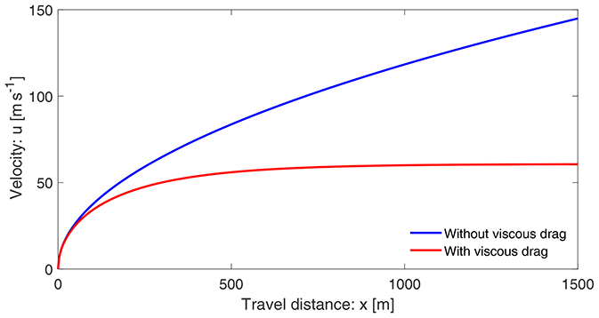
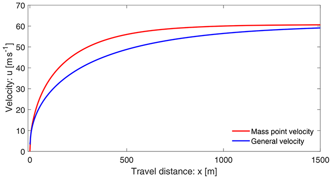
In what follows, unless otherwise stated, we use the plausibly chosen physical parameters for rapid mass movements: slope angle of about 50∘, , αs=0.65, and δ=20∘ (Mergili et al., 2020a, b; Pudasaini and Fischer, 2020). This implies the model parameters α=7.0 and β=0.0019. However, in principle, all of the results presented here are valid for any choice of the parameter set {α, β}. For simplicity, u0=0 is set at x0=0 at the position of the mass release. Figure 1 displays the velocity distributions of a landslide down the slope as a function of the slope position x. The magnitudes of the solutions presented here are mainly for reference purposes. For the orders of magnitude of velocities of natural events, we refer to Sect. 3.2.2. The velocities in Fig. 1 with and without drag already behave completely differently after the mass has moved a certain distance. For a relatively small travel distance, say x≤50 m, these two solutions are quite similar as the viscous drag is not sufficiently effective yet. The difference increases rapidly as the mass slides further down the slope. With the drag, the terminal velocity is attained at a sufficient distance. But, without drag, the velocity increases forever, which is less likely for a mass propagating down a long distance.
3.2 A mass point motion
Assume no or negligible local deformation (e.g., ) or a Lagrangian description; both are equivalent to the mass point motion. In this situation, only the ordinary differentiation with respect to time is involved, and can be replaced by . Then, the model (Eq. 5) reduces to
Perla et al. (1980) also called Eq. (10) the governing equation for the center of mass velocity but for a dry avalanche of flow type. This is a simple nonlinear first-order ordinary differential equation. This equation can be solved to obtain an exact analytical solution for the landslide velocity in terms of a tangent hyperbolic function (solution C):
where u0=u(t0) is the initial velocity at time t=t0. Equation (11) provides the time evolution of the velocity of the coherent (without fragmentation and substantial deformation) sliding mass until the time it fragments and/or moves like an avalanche. After that, we must use the full dynamical mass flow model (Pudasaini, 2012; Pudasaini and Mergili, 2019) or Eqs. (1) and (2). For more detail, see Sect. 6.1. For a sufficiently long time, the viscous force brings the motion to a non-accelerating state (steady, uniform). Then, from Eq. (11) we obtain
where stands for the terminal velocity of the motion of a point mass.
The landslide position
Since , Eq. (11) can be integrated to obtain the landslide position as a function of time:
where x0 corresponds to the position at the initial time t0.
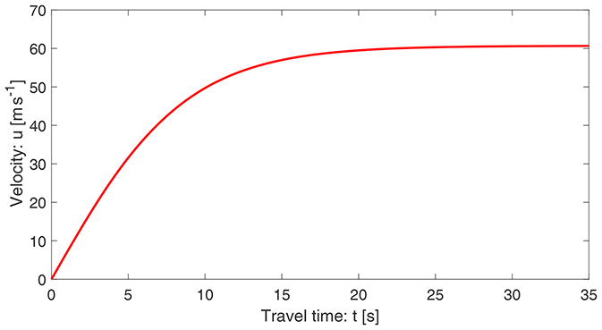
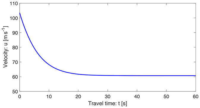
Figure 2 displays the velocity profile of a landslide as a function of time as given by Eq. (11). The terminal velocity is attained at a sufficiently long time (∼15 s). In the structure, the model (Eq. 10) and its solution (11) exist in the literature (Pudasaini and Hutter, 2007) and are classically called Voellmy's mass point model (Voellmy, 1955) or the Voellmy–Salm model (Salm, 1966) that disregards the position dependency of the landslide velocity (Gruber, 1989). But, (1−γ), αs, and the term associated with hg are new contributions not included in the Voellmy model, as well as K=1 therein, while in our consideration α and K can be chosen appropriately. Thus, the Voellmy model corresponds to the substantially reduced form of α, with .
3.2.1 The dynamics controlled by the physical and mechanical parameters
The solutions in Eqs. (8) and (11) are constructed independently: one for the velocity of a deformable mass as a function of travel distance, or the velocity of the center of mass of the landslide down the slope, and the other for the velocity of a mass point motion as a function of time. Unquestionably, they have their own dynamics. However, for a sufficiently long distance and sufficiently long time, or in the space and time limits, these solutions coincide and we obtain a unique relationship:
So, after a sufficiently long distance or a sufficiently long time, the forces associated with α and β always maintain a balance, resulting in the terminal velocity of the system, . Intuitively this is clear because one could simply imagine that a sufficiently long distance could somehow be perceived as a sufficiently long time, and for these limiting (but fundamentally different) situations, there is a single representative velocity that characterizes the dynamics. This has exactly happened and is an advanced understanding. This is shown in Figs. 1 and 2, which implicitly indicates the equivalence between Eqs. (8) and (11). In fact, this can be proven because for the mass point or the center of mass motion,
is satisfied.
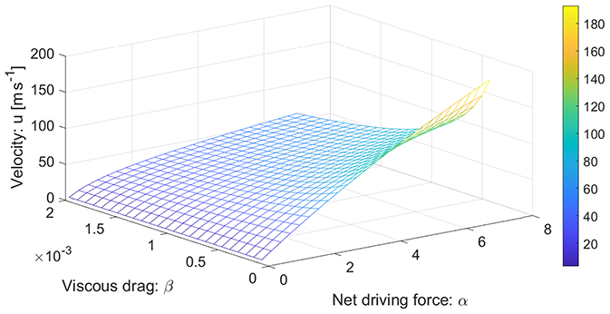
Figure 3The influence of the model parameters α and β on the landslide velocity. The color bar shows velocity distributions in meters per second (m s−1).
In Figs. 1 and 2, both velocities (with drag) have the same limiting values. The flow attains terminal velocity at about x=600 m and t=15 s, but their early behaviors are quite different. In space, the velocity shows a hyper-increase after the incipient motion. However, the time evolution of velocity is slow (almost linear) at first, then fast, and finally attains the steady state, m s−1, which is the common value for both the solutions.
3.2.2 The velocity magnitudes
A landslide can reach its maximum or terminal velocity after a relatively short travel distance or time with a value on the order of 50 m s−1 (Schaerer, 1975; Gubler, 1989; Christen et al., 2002; Havens et al., 2014). The velocity magnitudes presented above are quite reasonable for fast to rapid landslides and debris avalanches (Highland and Bobrowsky, 2008). The front of the 2017 Piz Cengalo–Bondo landslide already moved at more than 25 m s−1 20 s after of the rock avalanche release (Mergili et al., 2020b), and later it moved at about 50 m s−1 (Walter et al., 2020). The 1970 rock–ice avalanche event in Nevado Huascarán reached a mean velocity of 50–85 m s−1 at about 20 s, but the maximum velocity in the initial stage of the movement reached as high as 125 m s−1 (Erismann and Abele, 2001; Evans et al., 2009; Mergili et al., 2018). The 2002 Kolka glacier rock–ice avalanche accelerated with a velocity of about 60–80 m s−1 but also attained a velocity as high as 100 m s−1, mainly after the incipient motion (Huggel et al., 2005; Evans et al., 2009).
3.2.3 Accelerating and decelerating motions
Depending on the magnitudes of the involved forces and whether the initial mass was triggered with a small (including zero) velocity or with high velocity, e.g., by strong seismic shaking or when high potential energy is available and is converted quasi-instantaneously into kinetic energy (the situation prevails when the vertical height drop of the detachment area is huge and the slope angle of the terrain is high), Eq. (11) provides fundamentally different but physically meaningful velocity profiles. Both solutions asymptotically approach , which is the lead magnitude in Eq. (11). For notational convenience, we write , which has the dimension of velocity, and is called the separation number (velocity) as it separates accelerating and decelerating regimes. Furthermore, Sn includes all the involved forces in the system and is the function of the ratio between the mechanically known forces (i) gravity, friction, lubrication, and surface gradient as well as (ii) the viscous drag force coefficient. Thus, Sn fully governs the ultimate state of the landslide motion. For initial velocity less than Sn, i.e., u0<Sn, the landslide velocity increases rapidly just after its release, then ultimately (after a sufficiently long time) asymptotically approaches the steady state, Sn (Fig. 2). This is the accelerating motion. On the other hand, if the initial velocity was higher than Sn, i.e., u0>Sn, the landslide velocity would decrease rapidly just after its release and would then ultimately asymptotically approach Sn. This is the decelerating motion (not shown here).
3.2.4 Velocity described by the space of physical parameters
We now have two possibilities. First, we can describe as a function of time with α and β as parameters. This corresponds to the velocity profile of the particular landslide characterized by the geometrical, physical, and mechanical parameters α and β as time evolves. This is shown in Fig. 2. Second, we can investigate the control of the physical parameters on the landslide motion for a given time. This is achieved by plotting as a function of α and β and considering time as a parameter. Figure 3 shows the influence of α and β on the evolution of the velocity for a landslide motion for a typical time t=35 s. The parameters α and β enhance or control the landslide velocity completely differently. For a set of parameters {α, β}, we can now provide an estimate of the landslide velocity. As mentioned earlier, landslide velocities as high as 125 m s−1 have been reported in the literature, with their mean and common values in the range of 60–80 m s−1 for rapid motions. This way, we can explicitly study the influence of the physical parameters on the dynamics of the velocity field and also determine their range of plausible values. This answers the question of how the two similar-looking but physically differently characterized landslides would move. They may behave completely differently.
3.2.5 A model for viscous drag
There are explicit models for the interfacial drags between the particles and the fluid (Pudasaini, 2020) in the multi-phase mixture flow (Pudasaini and Mergili, 2019). However, there is no clear representation of the viscous drag coefficient for a landslide, which is the drag between the landslide and the environment. Often in applications, the drag coefficient (β=CDV) is prescribed and is later calibrated with numerical simulations to fit the observation or data (Kattel et al., 2016; Mergili et al., 2020a, b). Here, we explore an opportunity to investigate how the characteristic landslide velocity (Eq. 14) offers a possibility to define the drag coefficient. Equation (14) can be written as
where umax represents the maximum possible velocity during the motion as obtained from the (long-time) steady-state behavior of the landslide. Equation (16) provides a clear and novel definition (representation) of the viscous drag in mass movement (flow) as the ratio of the applied forces to the square of the steady-state (or a maximum possible) velocity the system can attain. With the representative mass m, Eq. (16) can be written as
Equivalently, β is the ratio between one-half of the “system force”, (the driving force), and the (maximum) kinetic energy, , of the landslide. With the knowledge of the relevant maximum kinetic energy of the landslide (Körner, 1980), the model (Eq. 17) for the drag can be closed.
3.2.6 Landslide motion down the entire slope
Furthermore, we note that following the classical method by Voellmy (Voellmy, 1955) and extensions by Salm (1966) and McClung (1983), the velocity models in Eqs. (8) and (11) can be used for multiple slope segments to describe the accelerating and decelerating motions as well as the landslide run-out. These are also called the release, track, and run-out segments of the landslide or avalanche (Gubler, 1989). However, for the gentle slope, or the run-out, the frictional force may dominate gravity. In this situation, the sign of α in Eq. (5) changes. Then, all the solutions derived above must be thoroughly revisited with the initial condition for velocity obtained from the lower end of the upstream segment. This way, we can apply the model (Eq. 5) to analytically describe the landslide motion for the entire slope from its release through the track and the run-out, as well as to calculate the total travel distance. These methods can also be applied to the general solutions derived in Sects. 4 and 5.
We mention that, for two-dimensional cycloidal or parabolic tracks, Gauer (2018) presented analytical velocities for the mass block motions with simple dry Coulomb or constant energy dissipation along the track. For such idealized path geometries he found an important relationship: the maximum front velocity, Umax, of major snow avalanches scales with the total drop height of the track, Hsc:, where g is the gravity constant. Within its scope, this simple relationship may be applied to estimate the maximum velocity in Eq. (17).
For shallow motion the velocity may change locally, but the change in the landslide geometry may be parameterized. In such a situation, the force produced by the free-surface pressure gradient can be estimated. A particular situation is the moving slab for which hg=0; otherwise, hg≠0. This justifies the physical significance of Eq. (5).
The Lagrangian description of a landslide motion is easier. However, the Eulerian description provides a better and more detailed picture as it also includes the local deformation due to the velocity gradient. So, here we consider the model equation (Eq. 5). Without reduction, conceptually, this can be viewed as an inviscid, nonhomogeneous, dissipative Burgers' equation with a quadratic source of system forces, and it includes both the time and space dependencies of u. Exact analytical solutions for Eq. (5) can still be constructed, but in more sophisticated forms, and are very demanding mathematically. For notational convenience, we rewrite Eq. (5) as
where g(u)=u and correspond to our model
(Eq. 5). Here, g and f are sufficiently smooth functions of u, the landslide velocity. We construct an exact analytical solution to the
generic model (Eq. 18). For this, first we state the following theorem from Nadjafikhah (2009).
Theorem 4.1: Let f and g be invertible real-valued functions of real variables; f is away from zero everywhere, is invertible, and
. Then, is the solution of Eq. (18), where F is an arbitrary real-valued smooth function of t−ϕ(u).
For our problem (Eq. 5), we have constructed the exact analytical solution (in Sect. 4.1), and it reads as (solution D)
describing the temporal and spatial evolution of the landslide velocity. It is important to note that in Eq. (19), the major role is played by the function ϕ that contains all the forces of the system. Furthermore, the function F includes the time dependency of the solution. The amazing fact with the solution (Eq. 19) is that any smooth function F with its argument [t−ϕ(u)] is a valid solution of the model equation. This means that different landslides may be described by different F functions. Alternatively, a class of landslides might be represented by a particular function F. This is substantial.
4.1 Derivation of the solution to the general model equation
Here, we present the detailed derivation of the analytical solution (Eq. 19) to the landslide velocity equation (Eq. 5). We derive the functions ϕ, ϕ−1, l, and loϕ that are involved in Theorem 4.1. The first function ϕ is given by
With the substitution τ=ϕ(u) (which implies ), we obtain
So, now the second function ϕ−1 can be written in terms of u. However, we must be consistent with the physical dimensions of the involved variables and functions. The quantities u, , , and τ have dimensions of m s−1, s−1, m s−1, and s. Thus, for dimensional consistency, the following mapping introduces a new multiplier λ with the dimension of 1 m s−2. Therefore, we have
With this, the third function l(u) yields
The fourth function l(ϕ(u))=(loϕ)(u) is instantly achieved:
where, as before, the multipliers χ and ξ emerge due to the transformation, and for dimensional consistency, they have the dimensions of 1 (m s−2) and m s−2, respectively. The nice thing about the groupings () and (ξλ) is that they are now dimensionless and equal to unity.
Utilizing these functions in Theorem 4.1, we finally constructed the exact analytical solution (Eq. 19).
4.2 Recovering the mass point motion
The amazing fact is that the newly constructed general analytical solution (Eq. 19) is strong and includes both the mass point solutions for velocity (Eq. 11) and the position (Eq. 13). For this, consider a vacuum solution F(0)≡0, which implies t=ϕ(u). Then, with the functional relation of ϕ(u) in Eq. (19), we obtain
Up to the constant of integration parameters (with u0=0 at t0=0), Eq. (25) is Eq. (11). So, the first assertion is proved. Second, using F(0)≡0 and ϕ(u)=t in Eq. (19) immediately yields
Again, up to the constant of integration parameters (with x0=0 and u0=0 at t0=0), Eq. (26) is Eq. (13). This proves the second assertion.
Moreover, we mention that Eqs. (25) and (26) can also be obtained formally. This proves that the conditions used on F are legitimate. To see this, we differentiate Eq. (19) with respect to t to yield
But, differentiating ϕ in Eq. (19) with respect to t and employing Eq. (10), we obtain , or ϕ=t. Now, by substituting these in Eqs. (27) and (19) we respectively recover Eqs. (25) and (26).
However, we note that F in Eq. (19) is a general function. So, Eq. (19) provides a wide spectrum of analytical solutions for the landslide velocity as a function of time and space much wider than Eqs. (11) and (13).
4.3 Some particular exact solutions
Here, we present some interesting particular exact solutions of Eq. (19) in the limit as β→0. For this purpose, first we consider Eq. (5) with β→0 and introduce the new variables and . Then, Eq. (5) can be written as
We apply Theorem 4.1 to Eq. (28). So, f(u)=1 implies ϕ(u)=u, , and . Following the procedure as for Eq. (19), we obtain the solution to Eq. (28) as . However, the direct application of ϕ(u)=u in Eq. (19) leads to the solution (that is more complex in its form) . Then, in the limit, we must have
This is an important mathematical identity we obtained as a direct consequence of Theorem 4.1 and Eq. (19). Furthermore, the identity (Eq. 29) when applied to Eq. (26) implies
Thus, , which is the travel distance in time when the viscous drag is absent.
Moreover, with the definition of , for the particular choice of F≡0, results in , which is Eq. (7). Furthermore, with the choice of and , we obtain , which for small t can be approximated as u≈αt. But, in the limit as β→0, Eq. (11) brings about u=αt, which is valid for all t values. Thus, Eq. (19) generalizes both solutions in Eqs. (7) and (11) in numerous ways.
4.4 Reduction to the classical Burgers' equation
Interestingly, by directly taking the limit as β→0, from Eq. (19) we obtain
which can be written as
Importantly, for any choice of the function F, Eq. (32) satisfies
which reduces to the classical inviscid Burgers' equation when α→0.
4.5 Some explicit expressions for u in Eq. (19)
For a properly selected function F, Eq. (19) can be solved exactly for u. For example, consider a constant F, F=Λ. Then, an explicit exact solution is obtained as
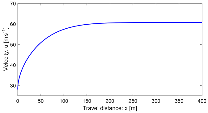
Figure 4 shows the velocity distribution given by Eq. (34) with u≈28 m s−1 at x=0 and Λ=0, which reaches the steady state at about x=150 m; this is faster than the solution given by Eq. (8) in Fig. 1. However, other more general solutions could be found by considering different F functions in Eq. (19).
For example, with , where c is a constant, Eq. (19) can be solved explicitly for u in terms of x and t:
The velocity profile along the slope as given by Eq. (35) is presented in Fig. 5 for t=1 m s−1 and c=1. This solution is quite different to that in Fig. 1 produced by Eq. (8). From the dynamical perspective, the solution (Eq. 35) is better than the mass point solution (Eq. 8). The important observation is that the solution given by Eq. (8) substantially overestimates the legitimate more general solution (Eq. 35) that includes both the local time and space variation of the velocity field. The lower velocity with Eq. (35) corresponds to the energy consumption due to the deformation associated with the velocity gradient in Eq. (5). This will be discussed in more detail in Sect. 4.6 and 4.7.
Furthermore, Fig. 6 presents the time evolution of the velocity field given by Eq. (35) for x=25 m and . This corresponds to the decelerating motion down the slope that starts with a very high velocity and finally asymptotically approaches the steady-state velocity.
4.6 Description of the general velocity
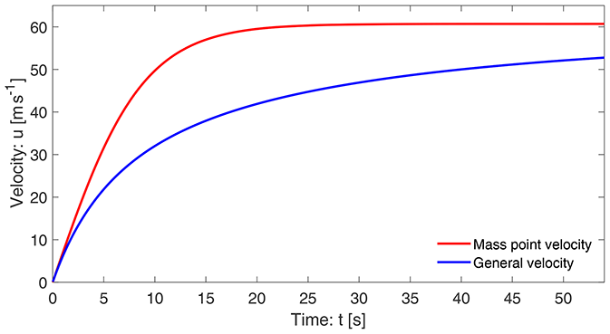
A crucial aspect of a complex analytical solution is its proper interpretation. The general solution (Eq. 19) can be plotted as a function of x and t. For the purpose of comparing the results with those derived previously, we select F as with parameter values Fk=5000, , and . Furthermore, x is a parameter while plotting the velocity as a function of t. In these situations, in order to obtain a physically plausible solution, is selected. To match the origin of the mass point solution, in plotting, the time has been shifted by −2. Figure 7 depicts the two solutions given by Eq. (11) for the mass point motion and the general solution given by Eq. (19) that also includes the internal deformation associated with in Eq. (5). They behave essentially differently right after the mass release. The mass point model substantially overestimates landslide velocity derived by the more realistic general model. However, the reduced dimensional models and solutions considered here may give upper bounds to reality because they do not account for the lateral spreading of the landslide mass. Such problems can only be solved comprehensively by considering the numerical simulations on a full three-dimensional digital terrain model (Mergili et al., 2020a, b; Shugar et al., 2021) and employing the full dynamical mass flow model equations (Pudasaini and Mergili, 2019) without constraining the lateral spreading.
4.7 A fundamentally new understanding
The new general solution (Eq. 19) and its plot in Fig. 7 provide a fundamentally new aspect in our understanding of landslide velocity. The physics behind the substantially, but legitimately, reduced velocity provided by the general velocity (Eq. 19) compared to the mass point velocity (Eq. 11) are revealed here for the first time. The gap between the two solutions increases steadily until a substantially large time (here about t=20 s); then the gap is reduced slowly. This is so because after t=20 s the mass point velocity is close to its steady value (about 60.1 m s−1). In the meantime, after t=20 s, the general velocity continues to increase but slowly, and after a long time, it also tends to approach the steady state. This substantially lower velocity in the general solution is realistic. Its mechanism can be explained. It becomes clear by analyzing the form of the model equation (Eq. 5). For ease of analysis, we assume accelerating flow down the slope. For such a situation, both u and are positive, and thus . The model (Eq. 5) can also be written as
Then, from the perspective of the time evolution of u, the last term on the right-hand side can be interpreted as a negative force additional to the system (Eq. 10) describing the mass point motion. This is responsible for the substantially reduced velocity profile given by Eq. (19) compared to that given by Eq. (11). The lower velocity in Eq. (19) can be perceived as the outcome of the energy consumed in the deformation of the landslide associated with the spatial velocity gradient that can also be inferred by the negative force attached with in Eq. (36). Moreover, in Eq. (5) can be viewed as the inertial term of the system (Bertini et al., 1994). However, after a sufficiently long time the drag is dominant, resulting in the decreased value of . Then, the effect of this negative force is reduced. Consequently, the difference between the mass point solution and the general solution decreases. However, these statements must be further scrutinized.
Below, we have constructed a further exact analytical solution to our velocity equation based on the method of Montecinos (2015). Consider the model (Eq. 5) and assign an initial condition:
This is a nonlinear advective–dissipative system and can be perceived as an inviscid, dissipative, nonhomogeneous Burgers' equation. First, we note that H(x) is a primitive of a function h(x) if . Then, we summarize the Montecinos (2015) solution method in a theorem.
Theorem 5.1: Let be an integrable function. Then, there exists a function ℰ(t,s0(y)) with its primitive ℱ(t,s0(y)) such that the initial value problem,
has the exact solution , where y satisfies .
Following Theorem 5.1, we obtain (in Sect. 5.1) the exact analytical solution (solution E) for Eq. (37):
where is given by
and provides the functional relation for s0(y). In contrast to Eq. (19), the system in Eqs. (39)–(40) is the direct generalization of the mass point solutions given by Eqs. (11) and (13). This is an advantage.
The solution strategy is as follows: use the definition of s0(y) in Eq. (40). Then, solve for y. Go back to the definition of s0(y) and put in s0(y). This s0(y) is now a function of x and t. Finally, put in Eq. (39) to obtain the required general solution for u(x,t). In principle, the system (Eqs. 39 and 40) may be solved explicitly for a given initial condition. One of the main problems in solving Eqs. (39) and (40) lies in inverting Eq. (40) to acquire y(x,t). Moreover, we note that, generally, Eqs. (19) and (39)–(40) may provide different solutions.
5.1 Derivation of the solution to the general model equation
The solution method involves some sophisticated mathematical procedures. However, here we present a compact but quick solution description to our problem. The equivalent ordinary differential equation to the partial differential equation system (Eq. 37) is
which has the solution
Consider a curve x in the x–t plane that satisfies the ordinary differential equation
Solving the system (Eq. 43), we obtain
So, the exact solution to the problem (Eq. 37) is given by
where y satisfies Eq. (44).
5.2 Recovering the mass point motion
It is interesting to observe the structure of the solutions given by Eqs. (39) and (40). For a constant initial condition, e.g., s0(x)=λ0, s0(y)=λ0, Eqs. (39) and (40) are decoupled. Then, Eq. (39) reduces to
For t=0, , which is the initial condition. Furthermore, Eq. (40) takes the form
from which we see that for t=0, , which is the initial position. With this, we observe that Eqs. (46) and (47) are the mass point solutions in Eqs. (11) and (13), respectively.

5.3 A particular solution
For the choice of the initial condition , combining Eqs. (39) and (40) leads to
which, surprisingly, is the same as the initial condition. However, we can now legitimately compare Eq. (48) with the previously obtained solution (Eq. 8), which is the steady-state motion with viscous drag. These two solutions are presented in Fig. 8. The very interesting fact is that Eqs. (8) and (48) turned out to be the same. For a real-valued parameter β and a real variable x, this reveals an important mathematically identity:
This means the very complex function on the left-hand side can be replaced by the much simpler function on the right-hand side. Moreover, taking the limit as β→0 in Eq. (48) and comparing it with Eq. (7), we obtain another functional identity:
These identities have mathematical significance.
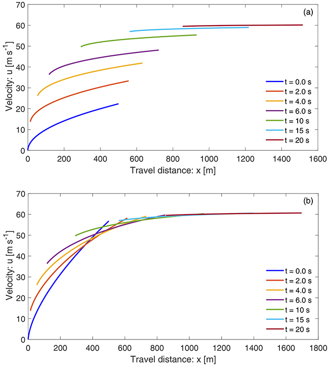
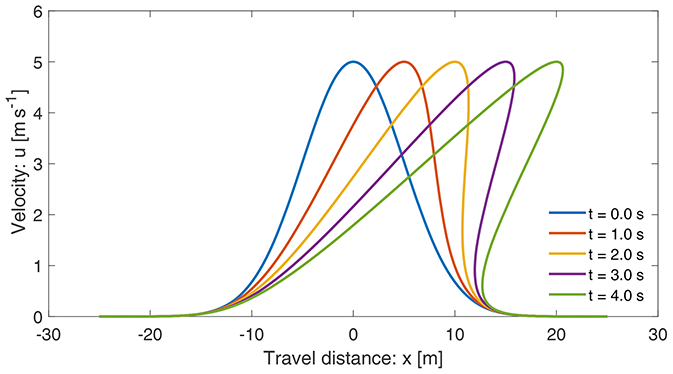
Figure 9Time evolution of velocity profiles of propagating and stretching landslides down a slope and as functions of position including the internal deformations as given by the general solution in Eqs. (39) and (40) of Eq. (5). The profiles evolve based on the initial conditions s0(x)=x0.50 (a, t=0.0 s) and s0(x)=x0.65 (b, t=0.0 s), respectively.
5.4 Time marching general solution
Any initial condition can be applied to the solution system (Eqs. 39 and 40). For the purpose of demonstrating the functionality of this system, here we consider two initial conditions: s0(x)=x0.50 and s0(x)=x0.65. The corresponding results are presented in Fig. 9. This figure clearly shows time marching of the landslide motion that also stretches as it slides down. Such deformation of the landslide stems from the term and the applied forces α−βu2 in our primary model (Eq. 5). We will elaborate on this later. This proves our hypothesis on the importance of the nonlinear advection and external forcing for the deformation and motion of the landslide. The mechanism and dynamics of the advection, stretching, and approaching the steady state can be explained with reference to the general solution. For this, consider panel b with initial condition s0(x)=x0.65. At t=0.0 s, Eq. (40) implies that y=x; then from Eq. (39), , which is the initial condition. Such a velocity field can take place in a relatively early stage of the developed motion of large natural events (Erismann and Abele, 2001; Huggel et al., 2005; Evans et al., 2009; Mergili et al., 2018). This is represented by the t=0.0 s curve. For the next time, say t=2.0 s, the spatial domain of u expands and shifts to the right as defined by the rule (Eq. 40). It has three effects in Eq. (39). First, due to the shift of the spatial domain, the velocity field u is relocated to the right (downstream). Second, because of the increased t value and the spatial term associated with tanh −1, the velocity field is elevated. Third, as the tanh function defines the maximum value of u (about 60.1 m s−1), the velocity field is controlled (somehow appears to be rotated). These dynamics also apply for t>2.0 s. These jointly produce beautiful spatiotemporal patterns in Fig. 9. Since the maximum of the initial velocity was already close to the steady-state value (the right end of the curve), the front of the velocity field is automatically and strongly controlled, limiting its value to 60.1 m s−1. So, although the rear velocity increases rapidly, the front velocity remains almost unchanged. After a sufficiently long time, t≥15 s, the rear velocity also approaches the steady-steady value. Then, the entire landslide moves downslope with virtually constant steady-state velocity, without any substantial stretching. We can similarly describe the dynamics for Fig. 9a. However, these two panels reveal an important fact: the initial condition plays an important role in determining and controlling the landslide dynamics.
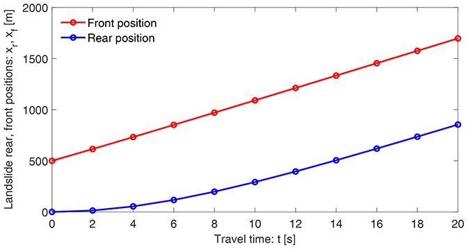
5.5 Landslide stretching
The stretching (or deformation) of the landslide propagating down the slope depends on the evolution of its front (xf) and rear (xr) positions with maximum and minimum speeds, respectively. This is shown in Fig. 10 corresponding to the initial condition s0(x)=x0.65 in Fig. 9. It is observed that the rear position evolves strongly nonlinearly, whereas the front position advances only weakly nonlinearly.
In order to better understand the rate of stretching of the landslide, in Fig. 11 we also plot the difference between the front and rear positions as a function of time. It shows the stretching (rate) of the rapidly deforming landslide. The stretching dynamic is determined by the front and rear positions of the landslide in time, as shown in Fig. 10. In the early stages, the stretching increases rapidly. However, in later times (about t≥15 s) it increases only slowly, and after a sufficiently long time, (the rate of) stretching vanishes as the landslide has already been fully stretched. This can be understood because after a sufficiently long time, the motion is in steady state. Nevertheless, the ways the two solutions reach the steady state are different. The two panels in Fig. 9 also clearly indicate that the stretching (rate) depends on the initial condition.
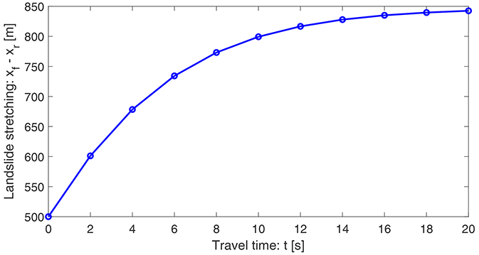
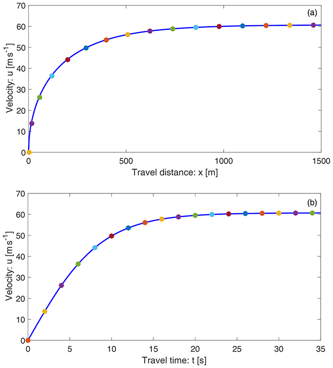
Figure 12Spatial (a) and temporal (b) transportations of the initial velocity (u=0) of the landslide down the slope by the general solution system (Eqs. 39 and 40) as indicated by the star markings for times t=0.0 s, with 2.0 s increments. These solutions exactly fit the space and time evolutions of the velocity fields (curves) for the mass point motions given by Eqs. (8) and (11).
5.6 Describing the dynamics
The dynamics observed in Figs. 9 and 11 can be described with respect to the general model in Eq. (5) or (37) and its solution given by Eqs. (39) and (40). The nice thing about Eq. (39) is that it can be analyzed in three different ways: with respect to the first or second or both terms on the right-hand side. If we disregard the first term involving time, then we explicitly see the effect of the second term that is responsible for the spatial variation of u for each time employed in Eq. (40). This results in the shift of the solution for u to the right, and in the meantime, the solution stretches but without changing the possible maximum value of u (not shown). Stretching continues for higher times; however, for a sufficiently long time, it remains virtually unchanged. On the other hand, if we consider both the first and second terms on the right-hand side of Eq. (39) but use the initial velocity distribution only for a very small x domain, say [0, 1], then we effectively obtain the mass point solutions given in Figs. 1 and 2 corresponding to Eqs. (8) and (11), respectively, for the spatial and time evolutions of u. This is so because now the very small initial domain for x essentially defines the velocity field as if it was for a center of mass motion. Then, as time elapses, the domain shifts to the right and the velocity increases. Now, plotting the velocity field as a function of space and time recovers the solutions in Figs. 1 and 2. In fact, if we collect all the minimum values of u (the left end points) in Fig. 9b and plot them in space and time, we acquire both the results in Figs. 1 and 2. These are effectively the mass point solutions for the spatial and time variation of the velocity field because these results only focus on the left end values of u, akin to the mass point motion. This means Eq. (40) together with Eq. (39) is responsible for the dynamics presented in Figs. 9–11 corresponding to the term and α−βu2 in the general model (Eqs. 5 or 37). So, the dynamics are specially architectured by the advection and controlled by the system forcing α−βu2 through the model parameters α and β. This will be discussed in more detail in Sect. 5.7–5.9. This reveals the fact that the shifting, stretching, and lifting of the velocity field stem from the term in Eq. (37). After a long time, as drag strongly dominates the other system forces, the velocity approaches the steady state, the velocity gradient practically vanishes, and thus the stretching ceases. Then, the landslide just moves down the slope at a constant velocity without any further dynamical complication.
5.7 Rolling out the initial velocity
It is compelling to see how the solution system (Eqs. 39 and 40) rolls out an initially constant velocity across specific curves. For this, consider an initial velocity s0(x)=0 in a small domain, say [0, 3], and take a point in it. Then, generate solutions for different times beginning with t=0.0 s, with 2.0 s increments. As shown in Fig. 12, the space and time evolutions of the velocity fields for a mass point motion given by Eqs. (8) and (11) have been exactly rolled up and covered by the system (Eqs. 39 and 40) by transporting the initial velocity along these curves (indicated by the star symbols). As explained earlier, the mechanism is such that, in time, Eq. (40) shifts the solution point (domain) to the right and Eq. (39) uplifts the velocity exactly lying on the mass point velocity curves designed by Eqs. (8) and (11). So, the system (Eqs. 39 and 40) generalizes the mass point motion in many different ways.
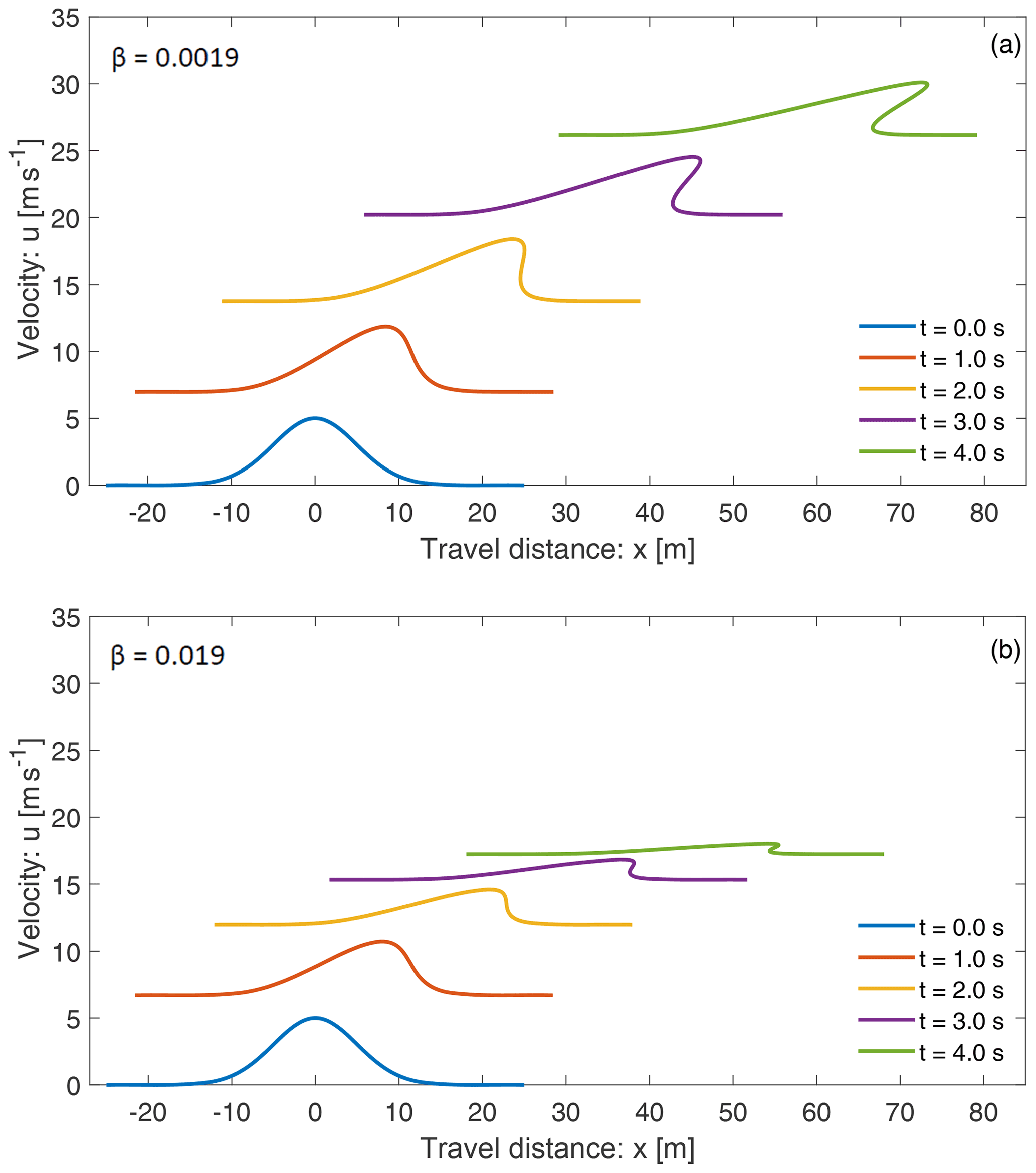
Figure 13The breaking wave and folding as a landslide propagates down a slope. Panel (a) has lower drag, while panel (b) has higher drag, showing that drag strongly controls the wave breaking and folding as well as the magnitude of the landslide velocity.
5.8 Breaking wave and folding
Next, we show how the new model (Eq. 5) and its solution system (Eqs. 39 and 40) can mold the breaking wave in mass transport and describe the folding of a landslide. For this, consider a sufficiently smooth initial velocity distribution given by . Such a distribution can be realized; e.g., as the landslide starts to move, its center might have been moving at the maximum initial velocity due to some localized strength weakening mechanism (examples include liquefaction, frictional strength loss, blasting, seismic shaking), and the strength weakening diminishes quickly away from the center. This later leads to a highly stretchable landslide from the center to the back, while from the center to the front, the landslide contracts strongly. The time evolution of the solution is presented in Fig. 13. Figure 13a is for the usual drag as before (β=0.0019), while Fig. 13b has higher drag (β=0.019). The drag strongly controls the wave breaking and folding, as well as the magnitude of the landslide velocity. Here, we focus on Fig. 13a, but similar analysis also holds for Fig. 13b.
Wave breaking and folding are often-observed important dynamical aspects in mass transport and formation of geological structures. Figure 13 reveals thrilling dynamics. The most fascinating feature is the velocity wave breaking and how this leads to the emergence of folding of the landslide. This can be explained with respect to the mechanism associated with the solution system (Eqs. 39 and 40). As is positive to the left and negative to the right of the maximum initial velocity, the motion to the left of the maximum initial velocity overtakes the velocity to the right of the maximum position. As the position of the maximum velocity accelerates downslope with the fastest speed, after a sufficiently long time, a kink around the front of the velocity wave develops, here after t=2 s. This marks the velocity wave breaking (shock wave formation) and the beginning of the folding. However, the rear stretches continuously. Although mathematically folding may refer to a singularity due to a multi-valued function, here we explain the folding dynamics as a phenomenon that can appear in nature. In time, the folding intensifies, and the folding length increases, but the folding gap decreases. After a long time, the folding gap virtually vanishes and the landslide moves downslope at the steady-state velocity with a perfect fold in the frontal part (not shown), while in the back, it maintains a single large stretched layer. This happened collectively as the system (Eqs. 39 and 40) simultaneously introduced three components of the landslide dynamics: downslope propagation, velocity uplift, and breaking or folding in the frontal part while stretching in the rear. This physically and mathematically proves that nonuniform motion (with its maximum somewhere interior to the landslide) is the basic requirement for the development of the breaking wave and the emergence of landslide folding.
5.9 Recovering Burgers' model
As the external forcing vanishes, i.e., as α→0 and β→0, the landslide velocity equation (Eq. 5) reduces to the classical inviscid Burgers' equation. Then, for α→0 and β→0, one would expect that the general solution (Eqs. 39 and 40) should also reduce to the formation of the shock wave and wave breaking generated by the inviscid Burgers' equation. In fact, as shown in Fig. 14, this has exactly happened. For this, the solution domain remains fixed, and the solutions are not uplifted. This proves that Burgers' equation is a special case of our model (Eq. 5).
5.10 The viscous drag effect
It is important to understand the dynamic control of the viscous drag on the landslide motion. For this, we set α→0 but increased the value of the viscous drag parameter by 1 and 2 orders of magnitude. The results are shown in Fig. 15. In connection to Fig. 14, there are two important observations. First, the translation and stretching of the domain are solely dependent on the net driving force α, and when it is set to zero, the domain remains fixed. Second, the viscous drag parameter β effectively controls the magnitude of the velocity field and the wave breaking. Depending on the magnitude of the viscous drag coefficient, the generation of the shock wave and the wave breaking can be dampened (Fig. 15a) or fully controlled (Fig. 15b). Figure 15b further reveals that with a properly selected viscous drag coefficient, the new model can describe the deposition process of the mass transport and finally brings it to a standstill. In contrast to the classical inviscid Burgers' equation, due to the viscous drag effect, our model (Eq. 5) is dissipative and can be recognized as a dissipative inviscid Burgers' equation. However, here the dissipation is not due to the diffusion but due to the viscous drag.
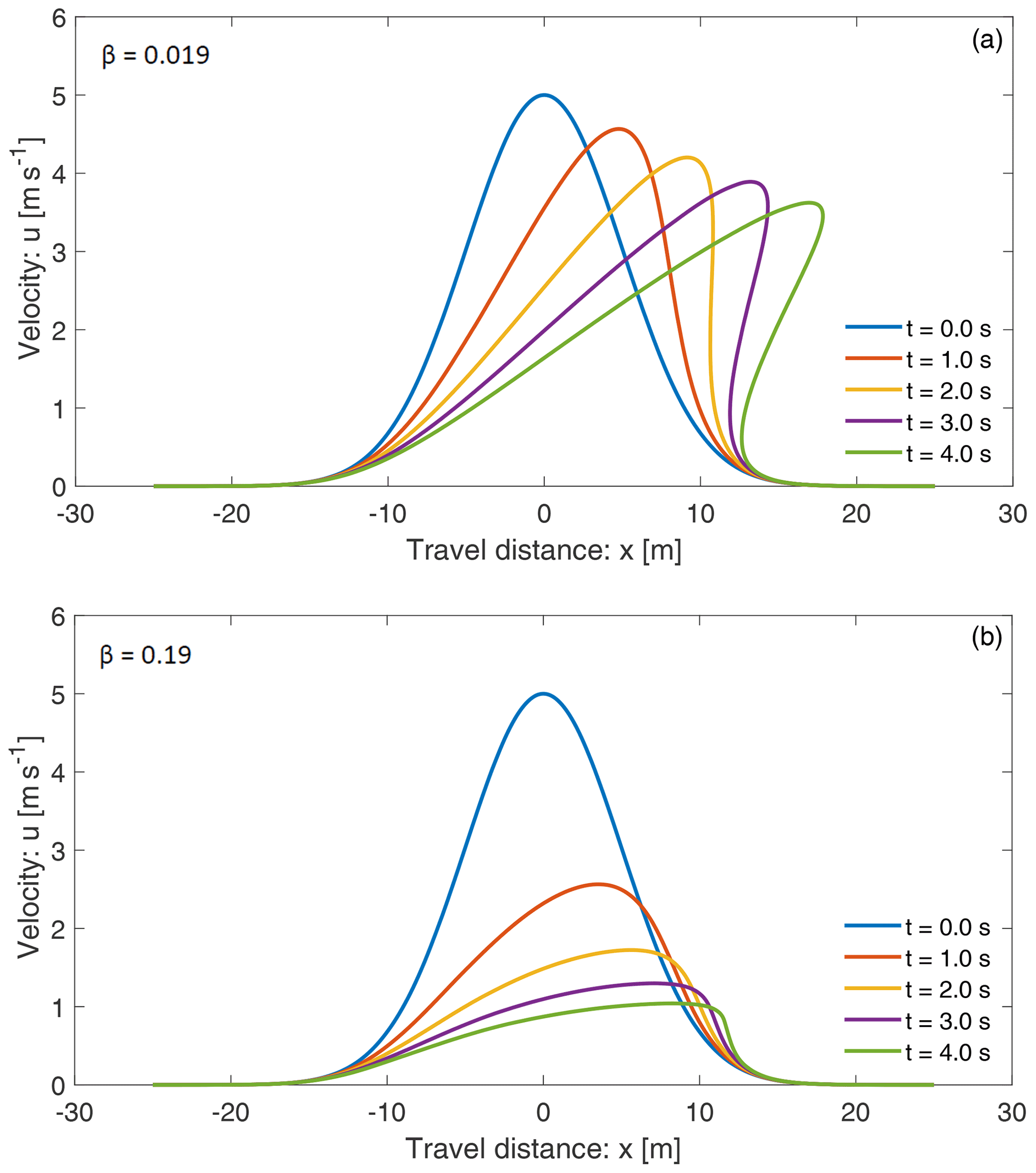
Figure 15The control of the viscous drag on the dynamics of the landslide. The net driving force is set to zero, i.e., α=0. The viscous drag has been amplified by 1 and 2 orders of magnitudes in panels (a) and (b), showing dampened or complete prevention of shock formation and wave breaking, respectively.
Exact analytical solutions of the underlying physical–mathematical models significantly improve our knowledge of the basic mechanism of the problem. On the one hand, such solutions disclose many new and essential physics and may thus find applications in environmental and engineering mass transports down natural slopes or industrial channels. The reduced and problem-specific solutions provide important insights into the full behavior of the complex landslide system, mainly the landslide motion with nonlinear internal deformation together with the external forcing. On the other hand, exact analytical solutions to simplified cases of nonlinear model equations are necessary to calibrate numerical simulations (Chalfen and Niemiec, 1986; Pudasaini, 2011, 2016; Ghosh Hajra et al., 2018). For this reason, this paper is mainly concerned about the development of a new general landslide velocity model and construction of several novel exact analytical solutions for landslide velocity.
Analytical solutions provide the fastest, cheapest, and probably the best solution to a problem as measured from their rigorous nature and representation of the dynamics. Proper knowledge of the landslide velocity is required in accurately determining the dynamics, travel distance, and enormous destructive impact energy carried by the landslide. The velocity of a landslide is associated with its internal deformation (inertia) and the externally applied system forces. The existing influential analytical landslide velocity models do not include many important forces and internal deformation. The classical analytical representation of the landslide velocity appear to be incomplete and restricted from both the physics and the dynamics point of view. No velocity model has been presented yet that simultaneously incorporates inertia and the externally applied system forces that play a crucial role in explaining important aspects of landslide propagation, motion, and deformation.
We have presented the first-ever physics-based, analytically constructed, simple but more general landslide velocity model. There are two main collective model parameters: the net driving force and drag. By rigorous derivations of the exact analytical solutions, we showed that incorporation of the nonlinear advection and external forcing is essential for the physically correct description of the landslide velocity. In this regard, we have presented a novel dynamical model for landslide velocity that precisely explains both the deformation and motion by quantifying the effect of nonlinear advection and the system forces.
Different exact analytical solutions for landslide velocity constructed in this paper independently support each other. These physically meaningful solutions can potentially be applied to calculate the complex nonlinear velocity distribution of the landslide. Our new results reveal that solutions to the more general equation for the landslide motion are widely applicable. The new landslide velocity model and its advanced exact solutions have made it possible to analytically study complex landslide dynamics, including nonlinear propagation, stretching, wave breaking, and folding. Moreover, these results clearly indicate that proper knowledge of the model parameters α and β is crucial in reliable prediction of the landslide dynamics.
6.1 Advantages of the new model and its solutions
The new model may describe the complex dynamics of many extended physical and engineering problems appearing in nature, science, and technology – connecting different types of complex mass movements and deformations. Specifically, the advantage of the new model equation is that the more general landslide velocity can now be obtained explicitly and analytically, which is very useful in solving relevant engineering and applied problems, and it has enormous application potential.
There are three distinct situations in modeling the landslide motion: (i) the spatial variation of the flow geometry and velocity can be negligible for which the entire landslide effectively moves as a mass point without any local deformation. This refers to the classical Voellmy model. (ii) The geometric deformation of the landslide can be parameterized or neglected; however, the spatial variation of the velocity field may play a crucial role in the landslide motion. In this circumstance, the landslide motion can legitimately be explained by the full form of the new landslide velocity equation (Eq. 5). The constructed general solutions in Eqs. (19) and (39)–(40) of this model have revealed many important features of dynamically deforming and advecting landslide motions. (iii) Both the landslide geometry and velocity may substantially change locally. Then, no assumptions on the spatial gradient of the geometry and velocity can be made. For this, only the full set of the basic model equations (Eqs. 1 and 2) can explain the landslide motion. While models and simulation techniques for situations (i) and (iii) are available in the literature, situation (ii) is entirely new both physically and mathematically. It is evident that dynamically situation (ii) plays an important role, first in making the bridge between the two limiting solutions and, second, by providing the most efficient solution. The solutions in Eqs. (19) and (39)–(40) include the local deformation associated with the velocity gradient. However, except for parameterization, Eqs. (19) and (39)–(40) do not explicitly include the geometrical deformation. As long as the spatial change in the landslide geometry is insignificant, we can use Eqs. (19) or (39) and (40) to describe the landslide motion. These solutions also include mass point motions and are valid before fragmentation and/or significant to large geometric deformations. However, when the geometric deformations are significant, we must use Eqs. (1) and (2) and solve them numerically with some high-resolution numerical methods (Tai et al., 2002; Mergili et al., 2017; 2020a, b).
The models in Eq. (19) or Eqs. (39)–(40) and Eqs. (1)–(2) are amicable and can be directly coupled. Such a coupling between the geometrically negligibly or slowly deforming landslide motion described by Eq. (19) or Eqs. (39)–(40) and the full dynamical solution with any large to catastrophic deformations described by Eqs. (1) and (2) is novel. First, this allows us to consistently couple the negligible or slowly deformable landslide with a fast (or rapidly) deformable flow-type landslide (or debris flow). Second, our method provides a very efficient simulation due to the instant exact solution given by Eq. (19) or Eqs. (39) and (40) prior to the large external geometric deformation that is then linked to the full model equations (Eqs. 1 and 2). Computational software such as r.avaflow (Mergili et al., 2017, 2020a, b; Pudasaini and Mergili, 2019) can substantially benefit from such a coupled solution method. Third, importantly, this coupling is valid for single-phase or multi-phase flows because the corresponding model (Eq. 5) is derived by reducing the multi-phase mass flow model (Pudasaini and Mergili, 2019).
Burgers' equation has no external forcing term. The solution domain remains fixed and does not stretch and propagate downslope. So, the initial velocity profile deforms and the wave breaks within the fixed domain. In contrast, our model (Eq. 5) is fundamentally characterized and explained simultaneously by the nonlinear advection and external forcing, α−βu2. The first designs the main dynamic feature of the wave, while the latter induces rapid downslope propagation, stretching of the wave domain, and quantification of the wave form and magnitude. These special features of our model are often-observed phenomena in mass transport and are freshly revealed here.
6.2 Compatibility, reliability, and generality of the solutions
Within their scopes and structures, many of the analytical solutions constructed in Sects. 3–5 are similar. This effectively implies the physical aspects of our general landslide velocity model (Eq. 5) and also the compatibility and reliability of all the solutions. The solutions in Eqs. (19) and (39)–(40) recover all the mass point motions given by Eqs. (11) and (13). From the physical and dynamical point of view, the velocity profiles given by Eqs. (19) and (39)–(40) as solutions of the general model for the landslide velocity (Eq. 5) are much wider and better than those given by Eqs. (11) and (13) as solutions of the mass point model (Eq. 10).
Structurally, the solutions presented in Sect. 3 are only partly new, yet they are physically substantially advanced. However, in Sects. 4 and 5 we have presented entirely novel solutions both physically and structurally. From a physical and mathematically point of view, particularly important is the form of the general velocity model (Eq. 5). First, it extends the classical Voellmy mass point model (Voellmy, 1955) by including (i) much wider physical aspects of landslide types and motions as well as (ii) the landslide dynamics associated with the internal deformation as described by the spatial velocity gradient associated with the advection. Second, the model (Eq. 5) is the direct extension of the inviscid Burgers' equation by including a (quadratic) nonlinear source as a function of the state variable. This source term contains all the applied forces appearing from the physics and mechanics of the landslide motion.
Moreover, as viewed from the general structure of the model (Eq. 5), all the solutions constructed here can be utilized for any physical problems that can be cast and represented in form (Eq. 5), but independent of the definition of the model parameters α and β, as well as the state variable u (Faraoni, 2022).
6.3 Implications
The new model (Eq. 5) and its solutions have broad implications mathematically, physically, and technically. By deriving a general landslide velocity model and its various analytical exact solutions, we made a breakthrough in correctly determining the velocity of a deformable landslide that is controlled by several applied forces as it propagates down the slope. We achieve a novel understanding that the inertia and the forcing terms ultimately regulate the landslide motion and provide a physically more appropriate analytical description of landslide velocity, dynamic impact, and inundation. This addresses the long-standing scientific question of explicit and full analytical representation of the velocity of deformable landslides. Such a description of the state of landslide velocity is innovative.
As the analytically obtained values represent the velocity of natural landslides well, technically, this provides a very important tool for landslide engineers and practitioners in quickly, efficiently, and accurately determining landslide velocity. The general solutions presented here reveal an important fact: accurate information about the mechanical parameters, state of the motion, and initial condition is very important for the proper description of the landslide motion. We have extracted some interesting particular exact solutions from the general solutions. As direct consequences of the new general solutions, some important and nontrivial mathematical identities have been established that replace very complex expressions by straightforward functions.
While existing analytical landslide velocity models cannot deal with the internal deformation and mostly fail to integrate a wide spectrum of externally applied forces, we developed a simple but general analytical model that is capable of including both of these important aspects. In this paper, we (i) derived a general landslide velocity model applicable to different types of landslide motions, (ii) solved it analytically to obtain several exact solutions as a function of space and time for landslide motion, and (iii) highlighted the essence of the new model. The model includes the internal deformation due to nonlinear advection and the external nonlinear forcing consisting of the extensive net driving force and viscous drag. The model describes a dissipative system and involves dynamic interactions between the advection and external forcing that control the landslide deformation and motion. Our model constitutes a unique and new class of nonlinear advective–dissipative system with quadratic external forcing as a function of state variable, containing all system forces. The new equation may describe the dynamical state of many extended physical and engineering problems appearing in nature, science, and technology. There are two crucial novel aspects: first, it extends the classical Voellmy model and additionally explains the dynamics of a locally deforming landslide, providing a better and more detailed picture of the landslide motion. Second, it is a more general formulation but can also be viewed as an extended inviscid, nonhomogeneous, dissipative Burgers' equation by including the nonlinear source term as a quadratic function of the field variable. The source term accommodates the mechanics of an underlying problem through the net driving force and the dissipative viscous drag.
Due to the nonlinear advection and quadratic forcing, the new general landslide velocity model poses a great mathematical challenge to derive explicit analytical solutions. Yet, we constructed several new and general exact analytical solutions in more sophisticated forms. These solutions are strong, recover all the mass point motions in many different ways, and provide a much wider spectrum for the landslide velocity than the classical Voellmy and Burgers' solutions. The major role is played by the nonlinear advection and system forces. The general solutions provide essentially new aspects in our understanding of landslide velocity. We have also presented a new model for the viscous drag as the ratio between one-half of the system force and the relevant kinetic energy.
With the general solution, we revealed that different classes of landslides can be represented by different solutions under the roof of one velocity model. General solutions allowed us to simulate the progression and stretching of the landslide. We disclosed the fact that the shifting and stretching of the velocity field stem from the external forcing and nonlinear advection. After a long time, as drag strongly dominates the system forces, the velocity gradient vanishes, and thus the stretching ceases. Then, the landslide propagates down the slope just at a constant (steady-state) velocity. The general solution system can generate complex breaking waves in advective mass transport and describe the folding process of a landslide. Such phenomena have been presented and described mechanically for the first time. The most fascinating feature is the dynamics of the wave breaking and the emergence of folding. This happens collectively as the solution system simultaneously introduces three important components of the landslide dynamics: downslope propagation and stretching of the domain, velocity uplift, and breaking or folding in the frontal part while stretching in the rear. This physically proves that nonuniform motion is the basic requirement for the development of breaking wave and emergence of the landslide folding. This is a novel understanding. We disclosed the fact that the translation and stretching of the domain, as well as lifting of the velocity field, solely depend on the net driving force. Similarly, the viscous drag fully controls the shock wave generation, wave breaking, and folding, as well as the magnitude of the landslide velocity. Furthermore, the new model can describe the deposition or the halting process of the mass transport. As the external forcing vanishes, the general solution automatically reduces to the classical shock wave generated by the inviscid Burgers' equation. This proves that the inviscid Burgers' equation is a special case of our general model.
The theoretically obtained velocities are close to the often-observed values in natural events including landslides and debris avalanches. This indicates the broad application potential of the new landslide velocity model and its exact analytical solutions in quickly solving engineering and technical problems as well as in accurately estimating the impact force that is very important in delineating hazard zones and for the mitigation of landslide hazards.
The relevant data supporting the findings of this study are available within the paper.
The physical–mathematical models were developed by SPP, who also designed and wrote the paper, interpreted the results, and edited the paper through reviews. MK contributed to the discussions of the results with enhanced descriptions to better fit broader geosciences audiences.
At least one of the (co-)authors is a member of the editorial board of Earth Surface Dynamics. The peer-review process was guided by an independent editor, and the authors also have no other competing interests to declare.
Publisher's note: Copernicus Publications remains neutral with regard to jurisdictional claims in published maps and institutional affiliations.
Shiva P. Pudasaini acknowledges the financial support provided by the Technical University of Munich with the Visiting Professorship Program and the international research project AlpSenseRely – Alpine remote sensing of climate‐induced natural hazards – from the Bayerisches Staatsministerium für Umwelt und Verbraucherschutz, Munich, Bayern. We thank the reviewers and the associate editor Jens Turowski for their constructive comments and suggestions that helped to substantially improve the paper. We are grateful to Martin Mergili and Ivo Baselt for fruitful discussions. This paper is based on arXiv:2103.10939v1 at https://arxiv.org/pdf/2103.10939.pdf (Pudasaini and Krautblatter, 2021b).
This work was supported by the German Research Foundation (DFG) and the Technical University of Munich (TUM) in the framework of the Open Access Publishing Program.
This paper was edited by Jens Turowski and reviewed by two anonymous referees.
Baselt, I., de Oliveira, G. Q., Fischer, J.-T., and Pudasaini, S. P.: Evolution of stony debris flows in laboratory experiments, Geomorphology, 372, 107431, https://doi.org/10.1016/j.geomorph.2020.107431, 2021.
Berger, C., McArdell, B. W., and Schlunegger, F.: Direct measurement of channel erosion by debris flows, Illgraben, Switzerland, J. Geophys. Res.-Earth, 116, F01002, https://doi.org/10.1029/2010JF001722, 2011.
Bertini, L., Cancrini, N., and Jona-Lasinio, G.: The Stochastic Burgers Equation, Commun. Math. Phys., 165, 211–232, 1994.
Burgers, J. M.: A mathematical model illustrating the theory of turbulence, in: Advances in Applied Mechanics, edited by: von Mises, R. and von Karman, T., Academic Press Inc., New York, 171–199, https://doi.org/10.1016/S0065-2156(08)70100-5, 1948.
Cascini, L., Cuomo, S., Pastor, M., Sorbino, G., and Piciullo, L.: SPH run-out modelling of channelized landslides of the flow type, Geomorphology, 214, 502–513, 2014.
Chalfen, M. and Niemiec, A.: Analytical and numerical solution of Saint-Venant equations, J. Hydrol., 86, 1–13, 1986.
Christen, M., Bartelt, P., and Gruber, U.: AVAL-1D: an avalanche dynamics program for the practice, in: Vol. 2, 1st congress “Interpraevent in the Pacific Rim”, Conference proceedings “Protection of habitat against floods, debris flows and avalanches”, 14–18 October 2002, Matsumoto, Japan,, 715–725, https://www.dora.lib4ri.ch/wsl/islandora/object/wsl:17895 (last access: 6 March 2022), 2002.
Christen, M., Kowalski, J., and Bartelt, P.: Ramms: numerical simulation of dense snow avalanches in three-dimensional terrain, Cold Reg. Sci. Technol., 63, 1–14, 2010.
Cole, J. D.: On a quasi-linear parabolic equation occurring in aerodynamics, Quart. Appl. Math., 9, 225–236, 1951.
Cui, P., Zeng, C., and Lei, Y.: Experimental analysis on the impact force of viscous debris flow, Earth Surf. Proc. Land., 40, 1644–1655, 2015.
Cuomo, S., Pastor, M., Capobianco, V., and Cascini, L.: Modelling the space time evolution of bed entrainment for flow-like landslides, Eng. Geol., 212, 10–20, 2016.
de Haas, T. and van Woerkom, T.: Bed scour by debris flows: experimental investigation of effects of debris flow composition, Earth Surf. Proc. Land., 41, 1951–1966, 2016.
de Haas, T., Nijland, W., de Jong, S. M., and McArdell, B. W.: How memory effects, check dams, and channel geometry control erosion and deposition by debris flows, Scient. Rep., 10, 14024, https://doi.org/10.1038/s41598-020-71016-8, 2020.
Di Cristo, C., Iervolino, M., and Vacca, A.: Applicability of Kinematic and Diffusive models for mud-flows: a steady state analysis, J. Hydrol., 559, 585–595, 2018.
Dietrich, A. and Krautblatter, M.: Deciphering controls for debris-flow erosion derived from a liDAR-recorded extreme event and a calibrated numerical model (Rossbichelbach, Germany), Earth Surf. Proc. Land., 44, 1346–1361, 2019.
Dowling, C. A. and Santi, P. M.: Debris flows and their toll on human life: a global analysis of debris-flow fatalities from 1950 to 2011, Nat. Hazards, 71, 203–227, 2014.
Erismann, T. H. and Abele, G.: Dynamics of Rockslides and Rockfalls, Springer, New York, ISBN 978-3-662-04639-5, 2001.
Evans, S. G., Bishop, N. F., Smoll, L. F., Murillo, P. V., Delaney, K. B., and Oliver-Smith, A.: A re-examination of the mechanism and human impact of catastrophic mass flows originating on Nevado Huascaran, Cordillera Blanca, Peru in 1962 and 1970, Eng. Geol., 108, 96–118, 2009.
Faraoni, V.: Helmoltz problem for the Riccati equation from an analogous Friedmann equation, Eur. Phys. J. C, 82, 13, https://doi.org/10.1140/epjc/s10052-021-09966-0, 2022.
Faug, T.: Depth-averaged analytic solutions for free-surface granular flows impacting rigid walls down inclines, Phys. Rev. E, 92, 062310, https://doi.org/10.1103/PhysRevE.92.062310, 2015.
Faug, T., Chanut, B., Beguin, R., Naaim, M., Thibert, E., and Baraudi, D.: A simple analytical model for pressure on obstacles induced by snow avalanches, Ann. Glaciol., 51, 1–8, 2010.
Frank, F., McArdell, B. W., Huggel, C., and Vieli, A.: The importance of entrainment and bulking on debris flow runout modeling: examples from the Swiss Alps, Nat. Hazards Earth Syst. Sci., 15, 2569–2583, https://doi.org/10.5194/nhess-15-2569-2015, 2015.
Gauer, P.: Considerations on scaling behavior in avalanche flow along cycloidal and parabolic tracks, Cold Reg. Sci. Technol., 151, 34–46, 2018.
Ghosh Hajra, S., Kandel, S., and Pudasaini, S. P.: Optimal systems of Lie subalgebras for a two-phase mass flow, Int. J. Non-Lin. Mech., 88, 109–121, 2017.
Ghosh Hajra, S., Kandel, S., and Pudasaini, S. P.: On analytical solutions of a two-phase mass flow model, Nonlin. Anal. Real World Appl., 41, 412–427, 2018.
Gubler, H.: Comparison of three models of avalanche dynamics, Ann. Glaciol., 13, 82–89, 1989.
Havens, S., Marshall, H.-P., Johnson, J. B., and Nicholson, B.: Calculating the velocity of a fast-moving snow avalanche using an infrasound array, Geophys. Res. Lett., 41, 6191–6198, 2014.
Highland, L. M. and Bobrowsky, P.: The landslide handbook – A guide to understanding landslides: Reston, Virginia, US Geological Survey Circular 1325, US Gelogical Survey, p. 129, https://pubs.usgs.gov/circ/1325/ (last access: 6 March 2022), 2008.
Hopf, E.: The partial differential equation , Comm. Pure Appl. Math., 3, 201–230, 1950.
Huggel, C., Zgraggen-Oswald, S., Haeberli, W., Kääb, A., Polkvoj, A., Galushkin, I., and Evans, S. G.: The 2002 rock/ice avalanche at Kolka/Karmadon, Russian Caucasus: assessment of extraordinary avalanche formation and mobility, and application of QuickBird satellite imagery, Nat. Hazards Earth Syst. Sci., 5, 173–187, https://doi.org/10.5194/nhess-5-173-2005, 2005.
Iverson, R. M., Reid, M. E., Logan, M., Lahusen, R. G., Godt, J. W., and Griswold, J. P.: Positive feedback and momentum growth during debris-flow entrainment of wet bed sediment, Nat. Geosci., 4, 116–121, 2011.
Iverson, R. M. and Ouyang, C.: Entrainment of bed material by earth-surface mass flows: review and reformulation of depth-integrated theory, Rev. Geophys., 53, 27–58, 2015.
Johannesson, T., Gauer, P., Issler, D., and Lied, K.: The Design of Avalanche Protection Dams, Recent Practical and Theoretical Developments, edited by: Barbolini, M., Domaas, U., Harbitz, C. B., Johannesson, T., Gauer, P., Issler, D., Lied, K., Faug, T., and Naaim, M., European Commision, Directorate General for Research, ISBN 978-92-79-08885-8, 2009.
Kattel, P., Khattri, K., Pokhrel, P., Kafle, J., Tuladhar, B., and Pudasaini, S.,: Simulating glacial lake outburst floods with a two-phase mass flow model, Ann. Glaciol., 57, 349–358, 2016.
Kattel, P., Kafle, J., Fischer, J.-T., Mergili, M., Tuladhar, B. M., and Pudasaini, S. P.: Interaction of two-phase debris flow with obstacles, Eng. Geol., 242, 197–217, 2018.
Körner, H. J.: The Energy-Line Method in the Mechanics of avalanches, J. Glaciol., 26, 501–505, 1980.
Lanzoni, S., Gregoretti, C., and Stancanelli, L. M.: Coarse-grained debris flow dynamics on erodible beds, J. Geophys. Res.-Earth, 122, 592–614, 2017.
Le, L. and Pitman, E. B.: A model for granular flows over an erodible surface, SIAM J. Appl. Math., 70, 1407–1427, 2009.
Li, P., Hu, K., and Wang, X.: Debris flow entrainment rates in non-uniform channels with convex and concave slopes, J. Hydraul. Res., 56, 1–12, 2017.
Liu, W., Yang, Z., and He, S.: Modeling the landslide-generated debris flow from formation to propagation and run-out by considering the effect of vegetation, Landslides, 18, 43–58, 2021.
Lu, P. Y., Yang, X. G., Xu, F. G., Hou, T. X., and Zhou, J. W.: An analysis of the entrainment effect of dry debris avalanches on loose bed materials, SpringerPlus, 5, 1621, https://doi.org/10.1186/s40064-016-3272-4, 2016.
McClung, D. M.: Derivation of Voellmy's Maximum Speed and Run-Out Estimates from a Centre-of-Mass Model, J. Glaciol., 29, 350–352, 1983.
McCoy, S. W., Kean, J. W., Coe, J. A., Tucker, G. E., Staley, D. M., and Wasklewicz, T. A.: Sediment entrainment by debris flows: In situ measurements from the headwaters of a steep catchment, J. Geophys. Res., 117, F03016, https://doi.org/10.1029/2011JF002278, 2012.
McDougall, S. and Hungr, O.: Dynamic modelling of entrainment in rapid landslides, Can. Geotech. J., 42, 1437–1448, 2005.
Medina, V., Hürlimann, M., and Bateman, A.: Application of FLATModel, a 2D finite volume code, to debris flows in the northeastern part of the Iberian Peninsula, Landslides, 5, 127–142, 2008.
Mergili, M., Fischer, J.-T., Krenn, J., and Pudasaini, S. P.: r.avaflow v1, an advanced open-source computational framework for the propagation and interaction of two-phase mass flows, Geosci. Model Dev., 10, 553–569, https://doi.org/10.5194/gmd-10-553-2017, 2017.
Mergili, M., Emmer, A., Juricova, A., Cochachin, A., Fischer, J.-T., Huggel, C., and Pudasaini, S. P.: How well can we simulate complex hydro-geomorphic process chains? The 2012 multi-lake outburst flood in the Santa Cruz Valley (Cordillera Blanca, Peru), Earth Surf. Proc. Land., 43, 1373–1389, 2018.
Mergili, M., Pudasaini, S. P., Emmer, A., Fischer, J.-T., Cochachin, A., and Frey, H.: Reconstruction of the 1941 GLOF process chain at Lake Palcacocha (Cordillera Blanca, Peru), Hydrol. Earth Syst. Sci., 24, 93–114, https://doi.org/10.5194/hess-24-93-2020, 2020a.
Mergili, M., Jaboyedoff, M., Pullarello, J., and Pudasaini, S. P.: Back calculation of the 2017 Piz Cengalo–Bondo landslide cascade with r.avaflow: what we can do and what we can learn, Nat. Hazards Earth Syst. Sci., 20, 505–520, https://doi.org/10.5194/nhess-20-505-2020, 2020b.
Montecinos, G. I.: Analytic solutions for the Burgers equation with source terms, arXiv preprint: 1503.09079v1, 2015.
Nadjafikhah, M.: Exact solution of generalized inviscid Burgers' equation, arXiv preprint: 0908.3601v1, 2009.
Parez, S. and Aharonov, E.: Long runout landslides: a solution from granular mechanics, Front. Phys., 3, 80, https://doi.org/10.3389/fphy.2015.00080, 2015.
Perla, R., Cheng, T. T., and McClung, D. M.: A two-parameter model for snow-avalanche motion, J. Glaciol., 26, 197–207, 1980.
Pilvar, M., Pouraghniaei, M. J., and Shakibaeinia, A.: Two-dimensional sub-aerial, submerged, and transitional granular slides, Phys. Fluids, 31, 113303, https://doi.org/10.1063/1.5121881, 2019.
Pudasaini, S. P.: Some exact solutions for debris and avalanche flows, Phys. Fluids, 23, 043301, https://doi.org/10.1063/1.3570532, 2011.
Pudasaini, S. P.: A general two-phase debris flow model, J. Geophys. Res., 117, F03010, https://doi.org/10.1029/2011JF002186, 2012.
Pudasaini, S. P.: A novel description of fluid flow in porous and debris materials, Eng. Geol., 202, 62–73, 2016.
Pudasaini, S. P.: A full description of generalized drag in mixture mass flows, Eng. Geol., 265, 105429, https://doi.org/10.1016/j.enggeo.2019.105429, 2020.
Pudasaini, S. P. and Fischer, J.-T.: A mechanical erosion model for two-phase mass flows, Int. J. Multiphase Flow, 132, 103416, https://doi.org/10.1016/j.ijmultiphaseflow.2020.103416, 2020.
Pudasaini, S. P. and Hutter, K.: Avalanche Dynamics: Dynamics of Rapid Flows of Dense Granular Avalanches, Springer, Berlin, New York, ISBN 978-3-540-32687-8, 2007.
Pudasaini, S. P. and Krautblatter, M.: The mechanics of landslide mobility with erosion, Nat. Commun., 12, 6793, https://doi.org/10.1038/s41467-021-26959-5, 2021a.
Pudasaini, S. P. and Krautblatter, M.: The Landslide Velocity, arxiv: preprint, https://arxiv.org/pdf/2103.10939.pdf (last access: 7 March 2022), 2021b.
Pudasaini, S. P. and Mergili, M.: A multi-phase mass flow model, J. Geophys. Res.-Earth, 124, 2920–2942, 2019.
Pudasaini, S. P. and Miller, S. A.: The hypermobility of huge landslides and avalanches, Eng. Geol., 157, 124–132, 2013.
Pudasaini, S. P., Ghosh Hajra, S., Kandel, S., and Khattri, K. B.: Analytical solutions to a nonlinear diffusion-advection equation, Z. Angew. Math. Phys., 69, 150, https://doi.org/10.1007/s00033-018-1042-6, 2018.
Qiao, C., Ou, G., and Pan, H.: Numerical modelling of the long runout character of 2015 Shenzhen landslide with a general two-phase mass flow model, Bull. Eng. Geol. Environ. 78, 3281–3294, 2019.
Razis, D., Kanellopoulos, G., and der Weele, K.: The granular monoclinal wave, J. Fluid Mech., 843, 810–846, 2018.
Rui, Y. and Yin, M.: An Analytical Solution for the Run-Out of Submarine Debris Flows, Mar. Geod., 42, 246–262, 2019.
Saingier, G., Deboeuf, S., and Lagree, P.-Y.: On the front shape of an inertial granular flow down a rough incline, Phys. Fluids, 28, 053302, https://doi.org/10.1063/1.4948401, 2016.
Salm, B.: Contribution to avalanche dynamics, in: IAHS Publ. No. 69, International Symposium on Scientific Aspects of Snow and Ice Avalanches, 1965, Davos, 199–214, 1966.
Schaerer, P. A.: Friction coefficients and speed of flowing avalanches, in: IAHS-AISH Pub. 114, Snow Mechanics: Proceedings of the Grindelwald Symposium, April 1974, Int. Assoc. Sci. Hydro., 425–432, https://nrc-publications.canada.ca/fra/voir/td/?id=1d89f442-5be5-4c1c-bf84-ff3877e07189 (last access: 6 March 2022), 1975.
Scheidegger, A. E.: On the Prediction of the Reach and Velocity of Catastrophic Landslides, Rock Mech., 5, 231–236, 1973.
Schürch, P., Densmore, A. L., Rosser, N. J., and McArdell, B. W.: Dynamic controls on erosion and deposition on debris-flow fans, Geology, 39, 827–830, 2011.
Shugar, D. H., Jacquemart, M., Shean, D., et al.: A massive rock and ice avalanche caused the 2021 disaster at Chamoli, Indian Himalaya, Science, 373, 300–306, 2021.
Tai, Y.-C., Gray, J. M. N. T., Hutter, K., and Noelle, S.: Flow of dense avalanches past obstructions, Ann. Glaciol., 32, 281–284, 2001.
Tai, Y.-C., Noelle, S., Gray, J. M. N. T., and Hutter, K.: Shock-capturing and front-tracking methods for granular avalanches, J. Comput. Phys., 175, 269–301, 2002.
Theule, J. I., Liebault, F., Laigle, D., Loye, A., and Jaboyedoff, M.: Channel scour and fill by debris flows and bedload transport, Geomorphology, 243, 92–105, 2015.
Voellmy, A.: Über die Zerstörungskraft von Lawinen, in: Schweizerische Bauzeitung, Jahrg. 73, Ht. 12., 159–162; Ht. 15, 212–217; Ht. 17, 246–249: Ht. 19, 280–285, On the destructive force of avalanches, Translation No. 2, Alta, Avalanche Study Center, USDA, Forest Service, 1955.
Walter, F., Amann, S., Kos, A., Kenner. R., Phillips, M., de Preux, A., Huss, M., Tognacca, C., Clinton, J., Diehl, T., and Bonanomi, Y.: Direct observations of a three million cubic meter rock‐slope collapse with almost immediate initiation of ensuing debris flows, Geomorphology, 351, 106933, https://doi.org/10.1016/j.geomorph.2019.106933, 2020.
- Abstract
- Introduction
- Basic balance equation for landslide motion
- The landslide velocity: simple solutions
- The landslide velocity: general solution – I
- The landslide velocity: general solution – II
- Discussion
- Summary
- Code availability
- Author contributions
- Competing interests
- Disclaimer
- Acknowledgements
- Financial support
- Review statement
- References