the Creative Commons Attribution 4.0 License.
the Creative Commons Attribution 4.0 License.
 | 14 Mar 2022
Comparative analysis of the Copernicus, TanDEM-X, and UAV-SfM digital elevation models to estimate lavaka (gully) volumes and mobilization rates in the Lake Alaotra region (Madagascar)
Benjamin Campforts
Gerard Govers
Emilien Aldana-Jague
Vao Fenotiana Razanamahandry
Tantely Razafimbelo
Tovonarivo Rafolisy
Liesbet Jacobs
Over the past few decades, developments in remote sensing have resulted in an ever-growing availability of topographic information on a global scale. A recent development is TanDEM-X (TerraSAR-X add-on for digital elevation measurements), an interferometric synthetic aperture radar (SAR) mission of the Deutsche Zentrum für Luft- und Raumfahrt, providing near-global coverage and 12 m resolution digital elevation models (DEMs). Moreover, ongoing developments in uncrewed aerial vehicle (UAV) technology have enabled acquisitions of topographic information at a sub-meter resolution. Although UAV products are generally preferred for volume assessments of geomorphic features, their acquisition remains a time-consuming task and is spatially constrained. However, some applications in geomorphology, such as the estimation of regional or national erosion quantities of specific landforms, require data over large areas. TanDEM-X data can be applied at such scales, but this raises the question of how much accuracy is lost because of the lower spatial resolution. Here, we evaluated the performance of the 12 m TanDEM-X DEM to (i) estimate gully volume, (ii) establish an area–volume relationship, and (iii) determine mobilization rates through comparison with a higher-resolution (0.2 m) UAV structure-from-motion (SfM) DEM and a lower resolution (30 m) Copernicus DEM. We did this for six study areas in the Lake Alaotra region (central Madagascar), where lavaka (gullies) are omnipresent and surface area changes over the period 1949–2010s are available for 699 lavaka. Copernicus-derived lavaka volume estimates were systematically too low, indicating that the Copernicus DEM is too coarse to accurately estimate volumes of geomorphic features at the lavaka scale (100–105 m2). Lavaka volumes obtained from TanDEM-X were similar to UAV-SfM volumes for the largest features, whereas the volumes of smaller features were generally underestimated. To deal with this bias we introduce a breakpoint analysis to eliminate volume reconstructions that suffer from processing errors as evidenced by significant fractions of negative volumes. This elimination allowed the establishment of an area–volume relationship for the TanDEM-X data with fitted coefficients within the 95 % confidence interval of the UAV-SfM relationship. Our calibrated area–volume relationship enabled us to obtain large-scale lavaka mobilization rates ranging between 18 ± 3 and 311 ± 82 for the six different study areas, with an average of 108 ± 26 for the full dataset. These results indicate that current lavaka mobilization rates are 2 orders of magnitude higher than long-term erosion rates. With this study we demonstrate that the global TanDEM-X 12 m DEM can be used to accurately estimate volumes of gully-shaped features at the lavaka scale (100–105 m2), where the proposed breakpoint method can be applied without requiring the availability of a higher-resolution DEM. Furthermore, we use this information to make a first assessment of regional lavaka erosion rates in the central highlands of Madagascar.
Please read the corrigendum first before continuing.
-
Notice on corrigendum
The requested paper has a corresponding corrigendum published. Please read the corrigendum first before downloading the article.
-
Article
(6019 KB)
- Corrigendum
-
Supplement
(5436 KB)
-
The requested paper has a corresponding corrigendum published. Please read the corrigendum first before downloading the article.
- Article
(6019 KB) - Full-text XML
- Corrigendum
-
Supplement
(5436 KB) - BibTeX
- EndNote


Over the past few decades advanced technology has become increasingly available for the assessment of surface topography: structure-from-motion (SfM) algorithms applied to uncrewed aerial vehicle (UAV) imagery now allow centimeter-scale resolution, thereby revolutionizing the way we study Earth surface processes (Passalacqua et al., 2015; Tarolli, 2014; Clapuyt et al., 2016). Obtaining sub-meter-resolution digital elevation models (DEMs) from UAV-SfM still requires substantial fieldwork and is spatially limited due to the nature of the technology (Bangen et al., 2014). On the other hand, TanDEM-X (TerraSAR-X add-on for digital elevation measurements) is a spaceborne product with global coverage at 12 m resolution and, while being less detailed and accurate than these sub-meter-resolution DEMs, is a major step forward in comparison to 30 m resolution DEMs with a global coverage (Mudd, 2020).
This raises the question to which extent TanDEM-X imagery can be used to map three-dimensional morphological features requiring a higher degree of topographical detail over relatively large areas (> 10 km2). One example is the use of remotely sensed data to map the process of gully formation, which is known to significantly contribute to surface erosion (e.g., Poesen et al., 2003; Vanmaercke et al., 2021; Frankl et al., 2021). The mapping and monitoring of gully erosion was conventionally based on time-consuming and spatially limited field surveys (Castillo et al., 2012; Evans and Lindsay, 2010; Guzzetti et al., 2012). More recently, however, (sub-)meter-resolution DEMs have enabled the development of (semi-)automated gully delineation and volume determination methods (Niculiţă et al., 2020; Evans and Lindsay, 2010; Perroy et al., 2010; Eustace et al., 2009; Liu et al., 2016). TanDEM-X has, for example, already been successfully used for automatic gully detection (Vallejo Orti et al., 2019).
It is important to evaluate not only the extent to which TanDEM-X data can be used to estimate gully volumes but also its capacity to establish accurate area–volume relationships. This latter question is relevant since sub-meter-resolution surface imagery from a multitude of sources and moments in time is now globally and freely available through, for example, Google Earth (Fisher et al., 2012). This imagery can be used to identify geomorphic features and estimate their surface area with great detail. Area–volume or length–volume relationships then enable us to obtain estimates of volume changes over time when historical imagery from which areas or lengths can be derived is available. Work on gully and landslide erosion has shown that the establishment of these relationships enables us to estimate sediment mobilization rates (i.e., the average annual volume of hillslope material displaced per unit area) over large spatial and temporal scales (e.g., Malamud et al., 2004; Larsen et al., 2010; Hovius et al., 1997; Guzzetti et al., 2012; Broeckx et al., 2019; Frankl et al., 2013; Kompani-Zare et al., 2011). Furthermore, work on gully headcut retreat rates and associated sediment mobilization has indicated the importance of long measurement periods: large year-to-year variations result in very large (> 100 %) uncertainties over short (< 5 years) measuring periods (Vanmaercke et al., 2016).
Here, we evaluate the performance of TanDEM-X to estimate gully volumes and to establish area–volume relationships through comparison with a higher resolution (0.2 m) UAV-SfM DEM and a lower resolution (30 m) Copernicus DEM. The resolution of a DEM should be viewed in relation to the size of the landform, where sampling theory states that landforms should have dimensions of at least twice the DEM resolution (Theobald, 1989; Frankl et al., 2013). This would mean that a gully should have a theoretical minimum size of 0.16, 576, and 3600 m2 for the UAV-SfM, TanDEM-X, and Copernicus DEM, respectively, to be represented in the DEM. We used the lavaka of the central highlands of Madagascar as a case study. Lavaka are amphitheater-shaped gullies that are on average 60 m long, 30 m wide, and 15 m deep, with small outlets (Cox et al., 2010; Wells and Andriamihaja, 1993). They are omnipresent in the central highlands, leaving the landscape filled with “holes” (“lavaka” in Malagasy). Unlike other gullies, they typically lack surface feeder channels and tend to form on mid-slopes, broadening uphill through headward erosion (Wells et al., 1991; Wells and Andriamihaja, 1993). While Madagascar is often claimed to experience amongst the highest global erosion rates due to the presence of lavaka (Milliman and Farnsworth, 2011; Randrianarijaona, 1983), the amount of sediment that is directly produced by lavaka is currently unknown.
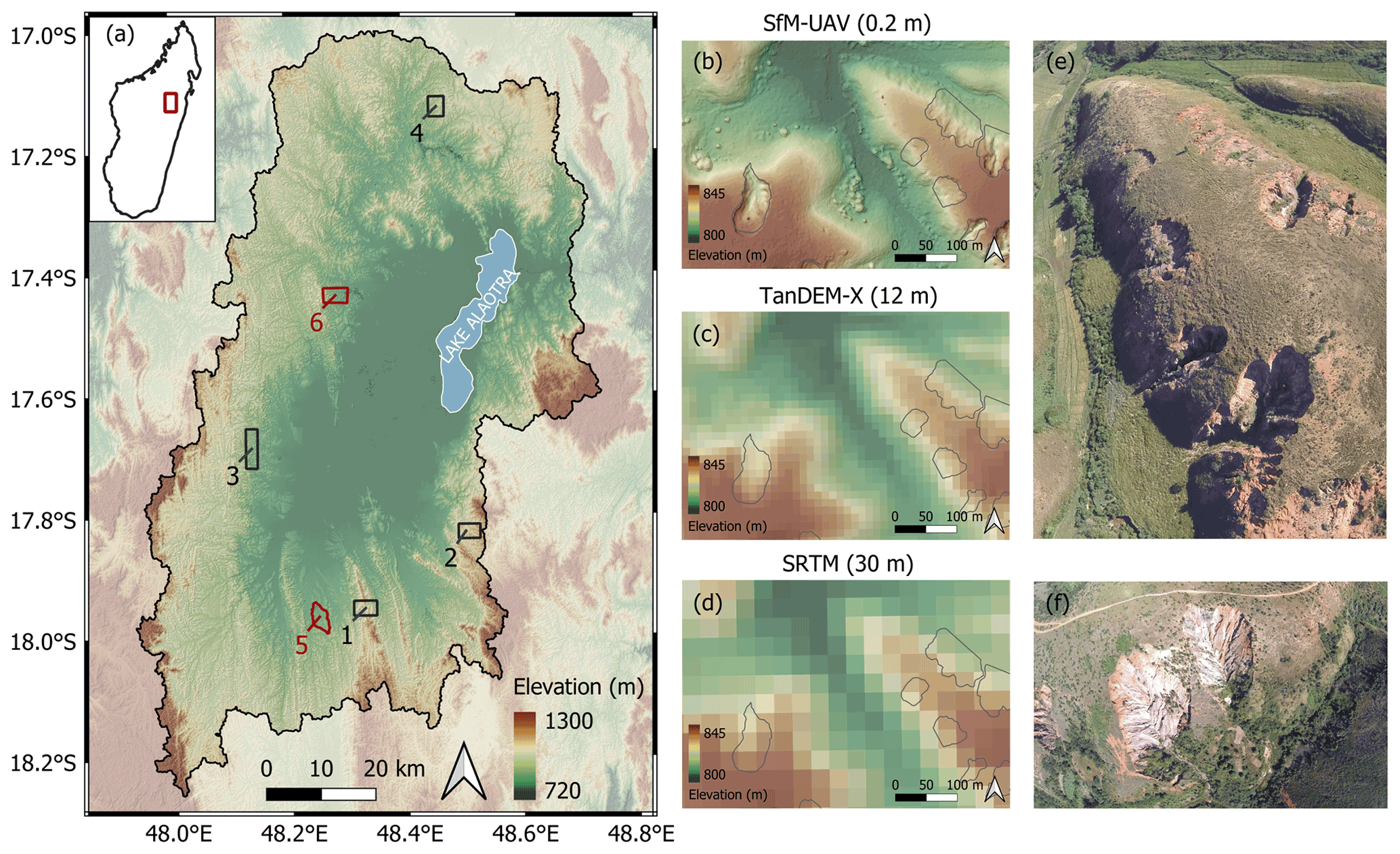
Figure 1Study areas, examples of each digital elevation model (DEM), and lavaka examples. (a) Six study areas of ca. 10 km2 in the Lake Alaotra catchment shown on the TanDEM-X DEM with hillshade. The UAV-SfM DEM is available for study area 5 and 6 (red) (data collected June 2018). (b–d) Examples of the Copernicus (AIRBUS, 2020a), TanDEM-X (Krieger et al., 2007), and UAV-SfM DEM (data collected June 2018) in SA6 located at 17∘58′51.7′′ S, 48∘15′18.6′′ E with hillshade. Grey outlines indicate the digitized lavaka. (e) UAV fisheye picture from 200 m height of the eastern ridge shown in (b–d). (f) UAV fisheye picture (200 m height) from two typical amphitheater-shaped lavaka (pictures taken in June 2018 by Liesa Brosens).
The objectives of our study are therefore to evaluate the performance of TanDEM-X to (i) estimate lavaka volumes, (ii) establish accurate area–volume relationships, and (iii) obtain a first estimate of lavaka mobilization rates. We derived lavaka volumes and mobilization rates for an existing dataset containing 699 digitized lavaka in six study areas in the Lake Alaotra region at three moments in time: 1949, 1969, and the 2010s. In a first step, lavaka volumes were calculated for the 2010s lavaka polygons from the DEM as the difference between a reconstructed pre-erosion surface and the current topography. Following this, a lavaka area–volume relationship was established between the current lavaka areas (2010s) and calculated volumes. Finally, this relationship was applied to the historical dataset with lavaka areas in 1949, 1969, and the 2010s. This enabled us to calculate lavaka volumes at each of these time steps and the consequent derivation of volumetric growth rates and lavaka mobilization rates for each of the six study areas. This procedure was followed for a 0.2 m resolution UAV-SfM DEM, the 12 m resolution TanDEM-X DEM, and the 30 m resolution Copernicus DEM.
2.1 Study area and lavaka dataset
Six study areas (SAs) of ca. 10 km2 were selected in the northeastern part of the central highlands of Madagascar in the area surrounding Lake Alaotra (Fig. 1a). The lake is located in the seismically active NE-SW oriented Alaotra–Ankay graben structure and is surrounded by convex-shaped, deeply weathered (> 10 m), and regolith-covered hillslopes that developed on the Precambrian crystalline basement (Kusky et al., 2010; Riquier and Segalen, 1949; Bourgeat, 1972; Mietton et al., 2018). The climate is characterized by a distinct dry and wet season with the regular occurrence of tropical cyclones. The mature rounded hillslopes are covered with open grasslands and contain one of the highest lavaka densities of the country, with up to 14 lavaka per square kilometer (Cox et al., 2010; Voarintsoa et al., 2012). The lowland areas bordering the lake consist of swamps in the SW and vast rice fields elsewhere, producing the majority of rice for the country (Lammers et al., 2015). For the six selected study areas, digitized lavaka polygons were generated from orthorectified and georeferenced historical aerial images from 1949 and 1969 (2.4 m resolution) and from recent (2011–2018, referred to as the 2010s) satellite imagery (WorldView-2, 0.5 m resolution) (Fig. 1a, Table S1 in the Supplement). All shapefiles have WGS84-UTM 39S (EPSG: 32739) coordinates. The dataset (available at https://doi.org/10.6084/m9.figshare.c.5236322.v1) contains the changes in surface area of 699 lavaka over the period 1949–2010s for SA1–5 and 1969–2010s for SA6. Each study area contains 50 to 173 lavaka, resulting in lavaka densities between 4 and 17 lavaka per square kilometer (Table S1).
2.2 Digital elevation models (DEMs)
Lavaka volumes were determined from three digital elevation models with a range of horizontal resolutions. For two study areas a 0.2 m resolution UAV-SfM DEM was obtained from a field campaign in 2018. For all study areas the 12 and 30 m resolution TanDEM-X and Copernicus DEMs are available. All DEMs were transformed to WGS84-UTM39S (EPSG: 32739) coordinates using a nearest-neighbor resampling method.
2.2.1 UAV-SfM DEM (0.2 m)
For study area 5 and 6 (Fig. 1a in red) a UAV field survey was carried out in June 2018 to obtain a 0.2 m resolution DEM. In order to cover a large area during a limited amount of time with a high spatial resolution, the post-processing kinematic (PPK) georeferencing approach as developed by Zhang et al. (2019) was used. The UAV images were directly georeferenced by using a RTK (real-time kinematic) receiver on the UAV that was connected to a RTK base station.
We used a custom-made quadcopter UAV with DJI N3 flight controller and fisheye action camera (Go Pro Hero 3, 12 megapixels, 4000 pixel × 3000 pixel, with a 2.92 mm F/2.8 123∘ HFOV lens). A compact Tallysman TW2710 multi-Global Navigation Satellite System (GNSS) RTK receiver antenna (Reach RTK kit, Emlid Ltd, 23 cm height) was mounted on an aluminum plate centered above the camera. The RTK receiver was connected to a single-board computer in order to synchronize the GPS time with the geotagging of the images. The RTK base station (Emlid Ltd) provided the positioning correction input. It was mounted on a tripod and located at a fixed position at the center of each study area during the flights. Flights were carried out at 200 m height at a speed of 8 m s−1. Pictures were taken every 3.8 s, resulting in an average ground sampling distance of 0.17 m (Fig. 1e and f).
The raw RTK-GPS data from the receiver were corrected with the data from the base station and post-processed using the RTKLib package (Takasu and Yasuda, 2009). A fix-and-hold method with 20∘ satellite elevation mask was used to correct the positions and geotag the images. The geotagged images were processed with Pix4D software using the default settings, with the vertical and horizontal accuracy set at 0.5 m. For the generation of the DEM, no surface smoothing or filtering was applied. The resulting DEM for both study areas has a resolution of ca. 0.2 m (Fig. 1b).
This method was reported to result in a robust and accurate alternative for georeferencing based on ground control points (GCPs) with a mean absolute error (MAE) of 0.02 m and root-mean-square error (RMSE) of 0.03 m for the vertical accuracy and a precision of 0.04 m (Zhang et al., 2019). Comparable studies over relatively flat areas with an UAV-RTK setup report similar vertical accuracies with RMSE values between 0.03 and 0.07 m (Taddia et al., 2020; Stott et al., 2020). UAV-SfM surveys with GCPs over more complex terrain report higher RMSE values of between 0.10 and 0.45 m (Clapuyt et al., 2016; Cook, 2017). Given the reported high accuracies of optical acquisitions that are georeferenced with RTK-GPS data, this DEM surface can be considered as the reference of the “true” elevation (Grohmann, 2018). In this study we therefore consider the UAV-SfM DEM as the ground-truth reference.
2.2.2 TanDEM-X DEM (12 m)
The TanDEM-X (TerraSAR-X add-on for digital elevation measurements) mission was launched in 2010 by the public–private partnership between the German Aerospace Center (DLR) and EADS Astrium GmbH (Krieger et al., 2007). Its configuration consists of two synthetic aperture radar (SAR) satellites flying in close formation and thereby forming a large X-band single-pass interferometer. The resulting global DEM has a horizontal resolution of 0.4 arcsec (ca. 12 m) and aims at < 2 m relative and < 10 m absolute vertical accuracy (Krieger et al., 2007, 2013; Wessel, 2016). The final TanDEM-X DEM was published in 2016 and consists of data collected between December 2010 and early 2015, where all land surfaces were imaged at least twice and up to 7 or 9 times in difficult terrain (Rizzoli et al., 2017, Fig. 1c). Our study areas were imaged 5 to 9 times, with an average of 7 ± 1, indicating a good coverage. The good performance of the TanDEM-X DEM has been reported, with a final global absolute vertical accuracy of 3.49 m and relative vertical accuracy of 0.99 and 1.37 m on flat (< 20∘) and steep (> 20∘) terrain, respectively (Rizzoli et al., 2017). These results are in line with Wessel et al. (2018) and Purinton and Bookhagen (2017), who reported absolute vertical accuracies of 0.20 ± 1.5 and −1.41 ± 1.97 m, respectively.
2.2.3 Copernicus DEM (30 m)
The 1 arcsec (ca. 30 m) resolution global Copernicus DEM (GLO-30) was released in 2021 by the European Space Agency (ESA) and AIRBUS. The DEM is based on the WorldDEM™, which is in turn based on edited and smoothed radar satellite data acquired during the TanDEM-X mission (AIRBUS, 2020a). The reported global absolute vertical accuracy is 2.17 m with an RMSE of 1.68 m. The relative vertical accuracy is smaller than 2 m for < 20∘ slopes and less than 4 m on > 20∘ slopes (AIRBUS, 2020b). Given its recent release, only limited additional validation has been carried out (Guth and Geoffroy, 2021). A lower absolute vertical accuracy of GLO-30 has been reported for mountainous areas in Europe with RMSE values between 7 and 14 m (Marešová et al., 2021). These estimates should, however, be viewed as maximum estimates as these high-relief terrains are one of the most challenging settings for DEM acquisitions. Upon comparison of different global 1 arcsec DEMs, Purinton and Bookhagen (2021) concluded that the Copernicus DEM provides the highest-quality landscape representation and should be the preferred DEM for topographic analysis in areas that lack higher-resolution DEMs. They furthermore report a high inter-pixel consistency for both the TanDEM-X and Copernicus DEM, indicating low relative vertical errors for these DEMs.
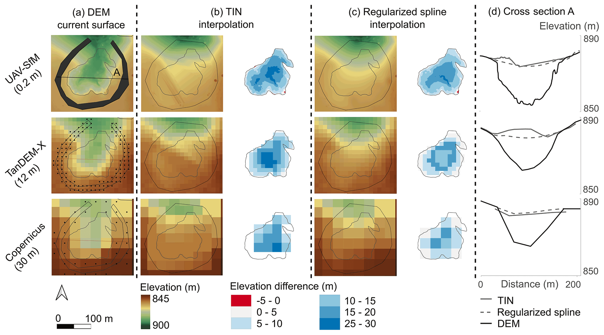
Figure 2Lavaka volume determination workflow. Lavaka volumes were calculated for each individual lavaka following an automated workflow for the three studied DEMs: UAV-SfM (0.20 m, top row, data collected June 2018), TanDEM-X (12 m, middle row, Krieger et al., 2007) and Copernicus (30 m, bottom row, AIRBUS, 2020a). (a) The digitized lavaka outline (grey), manually determined horseshoe-shaped polygon on the unaffected hillslope surrounding the lavaka, and current DEM are the three required inputs for the automated volume procedure. The DEM pixels that are not affected by erosion are clipped from the DEM with the horseshoe-shaped polygon and a single point per pixel is generated. The pre-erosion surface is then reconstructed by interpolating between these points (step 1). Two interpolation methods are shown as an example here: triangulated irregular network (TIN) (b) and regularized spline (c) interpolation. The grey polygon indicates the outer edge of the interpolated area. The elevation difference between the interpolated pre-erosion surface and current DEM surface is then calculated, which is clipped to the lavaka extent (Step 2–3). (d) Cross sections of transect A for the DEM, TIN, and regularized spline interpolation.
2.3 Lavaka volume quantification
Individual lavaka volumes were determined as the difference between the current surface and a reconstructed pre-erosion surface. This was done by developing an automated workflow in PyQGIS written in QGIS version 3.16.10 (code and example dataset available at https://doi.org/10.5281/zenodo.5768418). The automated PyQGIS workflow consists of four steps, which are explained in detail below.
- Input data
-
Three input files are required to run the automated volume procedure: (i) a shapefile containing the digitized lavaka (gully) outlines, (ii) a DEM raster file, and (iii) a shapefile containing the digitized outlines of the region surrounding the lavaka that is not affected by erosion. A manual delineation procedure was followed to obtain this surface unaffected by erosion, where a horseshoe-shaped polygon was drawn around each individual lavaka on the hillslope parts that were unaffected by erosion (Fig. 2a).
- Step 1: interpolate the pre-erosion surface
-
First, the DEM raster layer is clipped with the horseshoe-shaped polygon in order to extract the pixels not affected by gully erosion. All pixels that fall within this polygon are extracted in order to have a minimum width of one pixel. Next, one point per clipped DEM pixel is generated and used as input for the interpolation. Finally, these points are used to interpolate the pre-erosion surface. Five interpolation methods were tested, of which the method with the lowest error was applied to the lavaka dataset (see Sects. 2.4.1 and 3.1). Examples of the interpolated pre-erosion surface are shown in Fig. 2 for triangulated irregular network (TIN; see Fig. 2b) and regularized spline (Fig. 2c) interpolation.
- Step 2: calculate elevation difference
-
The current DEM is subtracted from the interpolated pre-erosion surface. The result is a difference raster, with positive values indicating a current surface that is lower than the reconstructed pre-erosion surface. Negative values indicate that the current topography is higher than the reconstructed topography.
- Step 3: elevation difference clipped to lavaka extent
-
The lavaka extent, which is given by the digitized lavaka polygons from the 0.5 m resolution WorldView-2 imagery from 2011–2018, is clipped from the elevation difference raster. In this way a raster with the elevation difference over the lavaka area is obtained (Fig. 2b and c). If the lavaka is smaller than a single pixel (0.04, 144, and 900 m2 for the UAV-SfM, TanDEM-X, and Copernicus DEM, respectively), the resulting raster is empty and no volume can be calculated.
- Step 4: export results
-
The unique value report of the lavaka elevation difference raster is exported. It contains the unique elevation values, their count, and the dimensions of the raster pixels. These results are used to calculate the volumes of each lavaka.
A manual delineation of the region surrounding the lavaka that is unaffected by erosion was preferred over an automated pre-erosion interpolation (e.g., Evans and Lindsay, 2010) or interpolation based on the lavaka outlines for two reasons. First, digitized lavaka outlines from aerial imagery are often located on DEM pixels that already have lower values. This is especially the case for the coarser-resolution DEMs due to surface smoothing (e.g., Fig. 1c and d). Second, the very dense presence of lavaka often results in a highly dissected topography and a near absence of topography not affected by lavaka erosion, requiring a precise identification of the areas not affected by erosion. For some lavaka, no horseshoe-shaped polygons could be delineated. In other cases, lavaka were grouped in one enveloping polygon when they were located next to each other (Fig. S1 in the Supplement).
The lavaka volume was calculated from the exported values report as the product of the elevation difference with the pixel area. Both positive and negative elevation differences occur, where a positive difference indicates that the current surface is lower than the reconstructed pre-erosion surface. Negative values indicate that the current topography is higher than the reconstructed topography. Given the presence of both positive and negative elevation differences, three types of volumes (V, m3) could be calculated for each lavaka: (i) the positive volume (Vpos) calculated by summing only the positive elevation differences, (ii) the negative volume (Vneg) calculated from the negative elevation differences, and (iii) the total volume (Vtot) as the difference between the positive and negative volume. If not further specified, the term “volume” refers to the positive volume.
The lavaka volumes as obtained from the different DEMs were compared in two ways: (i) pairwise comparison using only the lavaka for which the volume was determined for each DEM enabling a one-to-one comparison, and (ii) using all the data in order to establish the most robust relationships calibrated on a higher number of observations. The number of lavaka for which the volume was determined depends both on the availability of the UAV-SfM DEM (only in SA 5 and 6) and the resolution of the DEM. No volume could be calculated for the smallest features using the 12 and 30 m resolution DEMs.
2.4 Volume uncertainty assessment
Estimated lavaka volumes, determined as the difference between an interpolated pre-erosion surface and the current DEM surface, will entail a number of uncertainties and errors. Given our application, we address two types of uncertainty or error in our volume estimates: (i) the interpolation error and (ii) the relative height error of the DEM.
2.4.1 Interpolation error
The pre-erosion surface of the lavaka is reconstructed by interpolating between the DEM pixels (one point per pixel) that are not affected by gully erosion. While it is impossible to assess the real interpolation error for a lavaka, as the pre-erosion topography is simply unknown, this error can be estimated by interpolating the surface at locations where no lavaka are present and the pre-erosion surface is thus known. This method, which is similar to Bergonse and Reis (2015), not only allows us to estimate the uncertainties in derived lavaka volumes but also allows for the objective selection of the best interpolation method for a given topographic setting.
Five different lavaka polygons with sizes that span the range of our lavaka dataset were selected: 100, 1000, 5000, 10 000, and 20 000 m2. Each polygon was duplicated 10 times, resulting in 50 lavaka polygons. These polygons were placed on unaffected convex-shaped hillslopes on which lavaka typically occur, together with the corresponding horseshoe-shaped polygons. Our automated lavaka volume quantification method (Sect. 2.3) was then applied to this dataset using five different interpolation methods, where the difference between the interpolated surface and the DEM was calculated. This elevation difference gives the interpolation error, as a perfect interpolation would result in a surface identical to the original DEM.
We tested five commonly used interpolation methods for continuous data with their default parameter settings. The first two algorithms are based on a linear method where Delaunay triangles are constructed from the nearest neighbor points, resulting in non-smooth surfaces: (i) linear interpolation (GDAL, 2021) and (ii) TIN interpolation (QGIS, 2020). We also tested three spline interpolation methods that support the creation of curved surfaces in areas without data: (iii) bilinear spline (GRASS, 2021), (iv) bicubic spline (GRASS, 2021), and (v) regularized spline with tension (GRASS, 2003). The bilinear and bicubic spline interpolations are 2D piece-wise non-zero polynomial functions calculated within a limited 2D area, where the Tykhonov regularization parameter affects the smoothing of the surface (smoothing = 0.01). Linear spline is based on the use of 4 inputs to derive the coefficients, whereas bicubic spline uses 16 inputs, typically resulting in more precise outcomes (Brovelli et al., 2004; GRASS, 2021). In the regularized spline with tension algorithm (tension = 40, no smoothing) the tension parameter tunes the character of the resulting surface, from thin plate to membrane, and the smoothing parameter controls the deviation between points and the resulting surface (Mitášová and Mitáš, 1993; GRASS, 2003).
For all three DEMs and five interpolation methods the difference between the interpolated surface and DEM surface was calculated for the 50 lavaka polygons (example in Figs. S2 and S3). Based on the obtained height differences between the interpolated and original DEM surface, several error metrics were calculated (mean, median, RMSE, MAE, and standard deviation, i.e., SD), which were then used to (i) identify the best interpolation method and (ii) estimate the interpolation error. To estimate the interpolation error, it was verified whether the mean interpolation error of a lavaka depends on its area or not. If a significant relationship was absent, the mean ± SD interpolation error was used for all lavaka for that DEM. In the other case, where a relationship between lavaka area and mean lavaka interpolation error is present, we estimated the interpolation error based on the fitted linear relationship between both variables. Uncertainties in the fitted coefficients were taken into account by drawing 104 random Monte Carlo coefficient values from a normal distribution with known fitted mean and SD, where we used Gaussian copula to account for the correlation between both coefficients.
2.4.2 Relative height error
Typically, the performance of a DEM is assessed by considering its absolute vertical accuracy, i.e., the difference in DEM elevation and a high-resolution reference dataset (often lidar or Global Navigation Satellite System (GNSS) data points) (AIRBUS, 2020a; Wessel, 2016). In our application this absolute height error is, however, not the most important DEM error metric. Our volumes are the relative difference between the interpolated and real DEM, which is not influenced by the absolute vertical deviation of the DEM as long as this absolute deviation is the same for all considered pixels. We are instead interested in relative pixel-to-pixel errors, as these are more likely to affect the estimated volumes.
We assume this relative height error to be negligible for our 0.2 m resolution UAV-SfM DEM, given that the reported accuracy and precision values are on the order of a few centimeters (Zhang et al., 2019; Taddia et al., 2020; Stott et al., 2020). For the TanDEM-X and Copernicus DEM we use the height error masks (HEMs) that are provided as auxiliary files. The HEM gives the theoretical random height error for each pixel in the form of the standard deviation that results from the interferometric phase and the combination of different coverages. This error is considered to be a random error and does not include any contributions of systematic errors (Wessel, 2016; Wessel et al., 2018; AIRBUS, 2020a).
For each lavaka we calculated the mean ± SD HEM value, which we then use to estimate the relative DEM uncertainty. A positive correlation between mean HEM and lavaka area is observed, where larger lavaka have higher mean relative height uncertainties (Fig. S4a). By calculating the mean HEM for a lavaka we use the lavaka as the observational unit, as we also did for the interpolation error. By doing so we implicitly assume that all lavaka pixels are perfectly autocorrelated. This is further discussed in Text S1 in the Supplement.
2.4.3 Total uncertainty: Monte Carlo simulations
The total uncertainty for each lavaka volume is estimated by running 104 Monte Carlo simulations in which both the interpolation and relative height error are considered. For the relative height error we draw random values from the normal distribution with a mean of 0 and the SD being equal to the mean HEM of the lavaka. For the interpolation error we follow two different approaches depending on the presence or absence of a significant relationship between the mean interpolation error and lavaka area as detailed above (Sect. 2.4.1). The result of these Monte Carlo simulations are 104 volume estimates for each lavaka from which the mean and its uncertainty (standard deviation) are calculated.
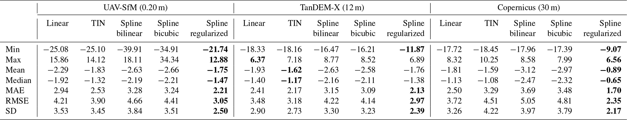
Table 1Interpolation error metrics. Minimum (min), maximum (max), mean, median, mean absolute error (MAE), root-mean-square error (RMSE), and standard deviation (SD) of the elevation differences between the interpolated and DEM surface for the 50 fictive lavaka polygons considering all pixels. The interpolation method yielding the lowest error is indicated in bold for each DEM and error metric.
2.5 Establishing area–volume relationships
Establishing a relationship between lavaka area and volume enables us to estimate lavaka volumes when only surface area information is available. Area–volume (typically landslides) and length–volume (typically gullies) relationships obey the following power law relationship: V=aAb, where the predicted volume V for a given area A depends on the scaling exponent a and intercept b (Larsen et al., 2010; Frankl et al., 2013). A linear relationship is typically fitted on the log-transformed data in order to obtain equally distributed residual errors, resulting in a more robust fit: (e.g., Guzzetti et al., 2009; Crawford, 1991). As lavaka typically have a specific inverse-teardrop shape and both lengthen and widen when they grow (Wells et al., 1991), we use lavaka area instead of length as a size measure. We have therefore established the relationship between lavaka area and volume by fitting a linear least-squares regression through the log-transformed data (base 10 log). The volumetric uncertainties are propagated into the area–volume relationship by fitting the linear relationship for all the 104 volume estimates from the Monte Carlo simulation and by calculating the mean and SD of the fitted a and b coefficients. These uncertainties are plotted as the 95 % confidence intervals and represent the expected variation in the mean estimated volume given a specific area. They do not represent the range in which the next individual volume estimate would fall given a specific area (i.e., the prediction interval). When back-transforming the coefficients of the fitted linear relationship to a power function, a systematic statistical bias enters. This is accounted for by adding a bias-correction factor that depends on the variance σ2 (Ferguson, 1986; Crawford, 1991) as follows: . This correction assumes that the residual errors of the fitted linear relationship are normally distributed with a mean of zero and variance σ2. The normal distribution of the residual errors was tested using a Shapiro–Wilk test (Shapiro and Wilk, 1965).
2.6 Lavaka volume growth and mobilization rates
From the established back-transformed area–volume relationship, lavaka volumes could be calculated using the surface areas of lavaka in 1949, 1969, and the 2010s, enabling the derivation of volumetric growth and mobilization rates. The volumetric growth rate (VGR, m3 yr−1) for each lavaka was calculated as the change in volume (dV, m3) over a given time period (dt, years):
where i indicates the most recent observation moment and j is the oldest observation moment.
Lavaka mobilization rates (LMR, ) give the amount of sediment that has been mobilized over a given period and area. LMR were calculated for each study area and are here expressed in tonnes per hectare per year. To obtain LMR, lavaka volumes were converted to mass using a dry bulk density (ρ) of 1.2 t m−3 (Montgomery, 2007). The sum of the lavaka masses of each study area was then divided by the length of the observation period and the surface area of the study area (A, ha):
where N is the number of lavaka in each study area.
Uncertainties in the calculated VGR and LMR were estimated by taking into account the uncertainties in the fitted a and b coefficients of the applied area–volume relationship. This was done by running 104 Monte Carlo simulations with different a and b values. These values were randomly drawn from the normal distribution of their mean and standard deviation. Gaussian copulas were used to take into account the dependence of both coefficients (Frees and Valdez, 1998). From all 104 runs the mean and standard deviation were calculated. All the calculated volumes, volumetric growth rates and mobilization rates are available at https://doi.org/10.5281/zenodo.5768418.
3.1 Interpolation methods and uncertainty
In order to select the best interpolation method and to quantify the interpolation error, 50 fictive lavaka polygons were placed on intact hillslopes and were interpolated by using five different interpolation methods. The resulting height differences then give the interpolation error (Figs. S2 and S3). When considering the results for the full dataset (all individual pixels, Table 1, Fig. S5) three main observations can be made. First, regularized spline interpolation has the smallest spread (SD, min, and max values) and lowest MAE and RMSE for all DEMs. The mean and median error are also lowest when using regularized spline interpolation for the UAV-SfM (−1.75 and −1.47 m) and Copernicus DEM (−0.89 and −0.65 m). However, for the TanDEM-X DEM, regularized spline interpolation results in slightly higher mean and median errors when compared to TIN interpolation (−1.76 and −1.38 m vs. −1.62 and −1.17 m). Second, the negative mean and median interpolation errors indicate that the interpolated surface is generally lower than the real surface. The interpolated pre-erosion surface is thus on average underestimated by −0.89 to −1.76 m, which will also result in a corresponding underestimation of the volume if this error is not accounted for. Third, all error metrics are highest for the highest-resolution DEM and decrease with decreasing resolution (e.g., RMSE decreases from 3.05 to 2.97 and 2.35 m for the UAV-SfM, TanDEM-X, and Copernicus DEM, respectively). Based on these results we conclude that the regularized spline method yields the best results overall in our landscape setting. We therefore apply this interpolation method to estimate the lavaka volumes.
Next, it was verified whether a significant relationship exists between the mean elevation difference of the 50 fictive lavaka polygons and their area (Fig. S6). Pearson correlation coefficients (ρ) indicate that a significant negative relationship is present for the UAV-SfM (ρ = −0.53, p = 8.14 × 10⁻⁵) and TanDEM-X DEM (ρ = −0.48, p = 1.53 × 10⁻³), which is absent for the Copernicus DEM (ρ = −0.10, p = 0.59). Therefore, the mean (± SD) elevation difference of −0.89 ± 2.17 m is used to incorporate the interpolation error for the Copernicus DEM in the Monte Carlo simulations (Table 1). For the UAV-SfM and TanDEM-X DEM the fitted linear relationship between the mean elevation difference and lavaka area and the corresponding uncertainties in the fitted coefficients are used to estimate the interpolation error in the Monte Carlo simulations (Fig. S6).
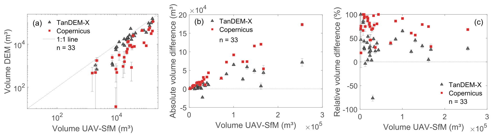
Figure 3Pairwise volume comparison. (a) Direct volume comparison between the lavaka volume obtained from the 0.2 m resolution UAV-SfM DEM and 12 and 30 m resolution TanDEM-X and Copernicus DEMs. The black line indicates the 1:1 line. Values are plotted on a log–log scale. (b) Absolute and (c) relative volume difference with the UAV-SfM DEM. The dotted horizontal line indicates the zero-difference level. Grey error bars are the standard deviations of the mean calculated volumes representing the total uncertainty (interpolation and relative DEM uncertainty).
3.2 Lavaka volumes
A direct pairwise comparison of the lavaka volumes obtained from the 0.2 m resolution UAV-SfM, 12 m resolution TanDEM-X, and 30 m Copernicus DEM indicates that Copernicus generally results in a large volume underestimation (Fig. 3a). TanDEM-X, on the other hand, results in fairly similar volume estimates as obtained by the UAV-SfM DEM, especially for the larger lavaka (> ca. 104 m3, Fig. 3a). While the absolute volume difference between UAV-SfM, TanDEM-X, and Copernicus increases with increasing lavaka volume (Fig. 3b), a different picture emerges when looking at the relative volume differences (Fig. 3c). The relative difference is largest for the smallest lavaka and decreases when lavaka become bigger. Both absolute and relative volume differences are largest for Copernicus, with strong volume underestimations for the smallest lavaka and relative underestimations generally remaining above 50 % for the larger features. For TanDEM-X, large relative differences also occur for the smallest lavaka; however, they decrease to less than 20 % for the largest features (Fig. 3c).
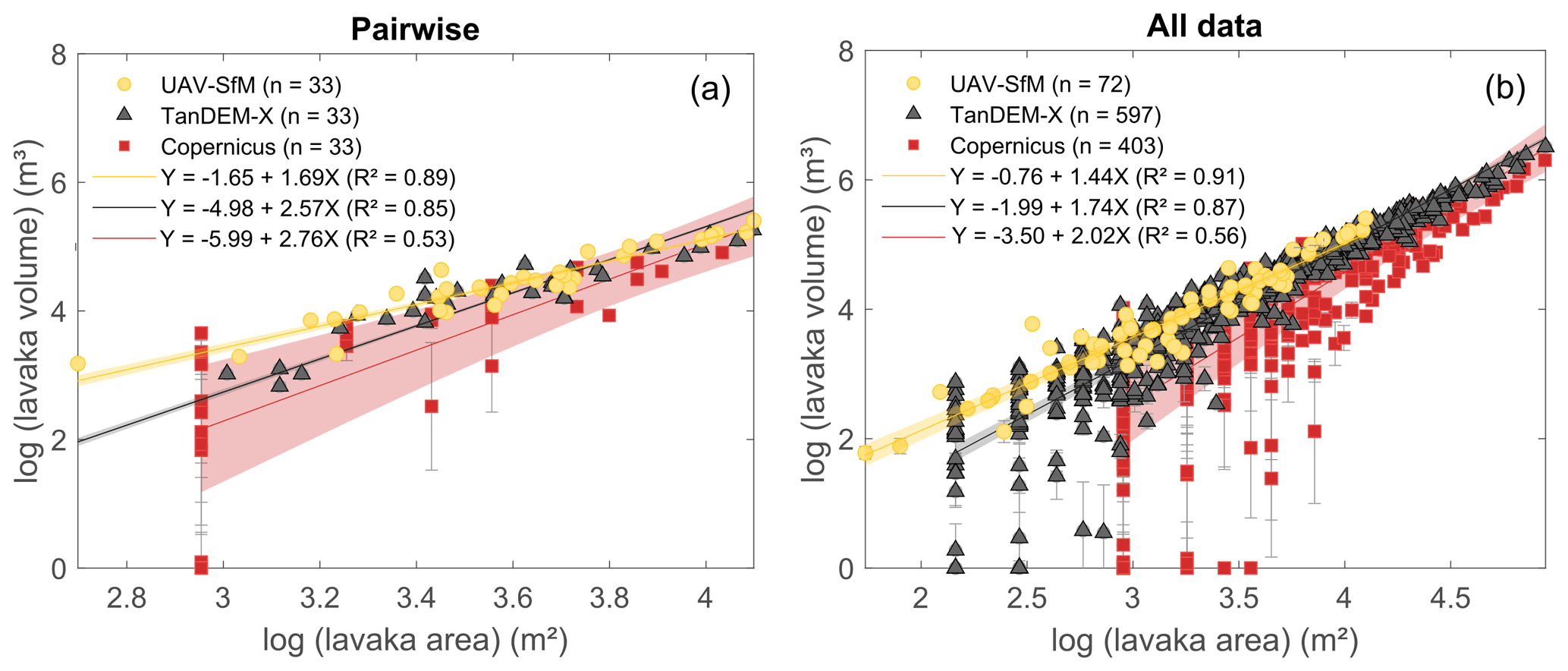
Figure 4Area–volume relationships. Fitted linear area–volume relationships between the log-transformed lavaka areas and volumes for (a) the pairwise dataset and (b) the full datasets containing all lavaka volumes for all three DEMs. Grey error bars are the standard deviations of the mean calculated volumes representing the total uncertainty (interpolation and relative DEM uncertainty). Shaded bands indicate the 95 % confidence intervals of the fitted relationships where the volumetric uncertainties are propagated through Monte Carlo simulations.
3.3 Area–volume relationships
Area–volume relationships were established using the log-transformed data. Both the relationships resulting from the pairwise and full dataset comparison clearly deviate for the different DEMs, where the smallest lavaka volumes are generally underestimated by TanDEM-X and Copernicus (Fig. 4). This results in a lower intercept and corresponding higher scaling exponent for the TanDEM-X and Copernicus relationships, which are significantly different (outside of the 95 % confidence interval) from the UAV-SfM relationship. This difference with the UAV-SfM relationship increases with decreasing DEM resolution and is largest for the Copernicus DEM (Fig. 4a). When considering the full dataset, large volume underestimations for the smallest lavaka are clearly apparent for volumes determined from the TanDEM-X and especially the Copernicus DEM (Fig. 4b). These are caused by negative volumes that were calculated over (a fraction) of the lavaka area. For larger lavaka areas and volumes this discrepancy with the UAV-SfM DEM disappears, suggesting that TanDEM-X and Copernicus are capable of accurately assessing lavaka volumes for features that exceed a given size (based on visual inspection of an area of ca. 103 and 104 m2 for the TanDEM-X and Copernicus DEM, respectively). However, because of the large volume underestimations for the smaller lavaka, the TanDEM-X and Copernicus area–volume relationships strongly deviate from the UAV-SfM relationship when incorporating all of the data, where the fitted coefficients are not within the confidence interval of the fitted UAV-SfM coefficients.
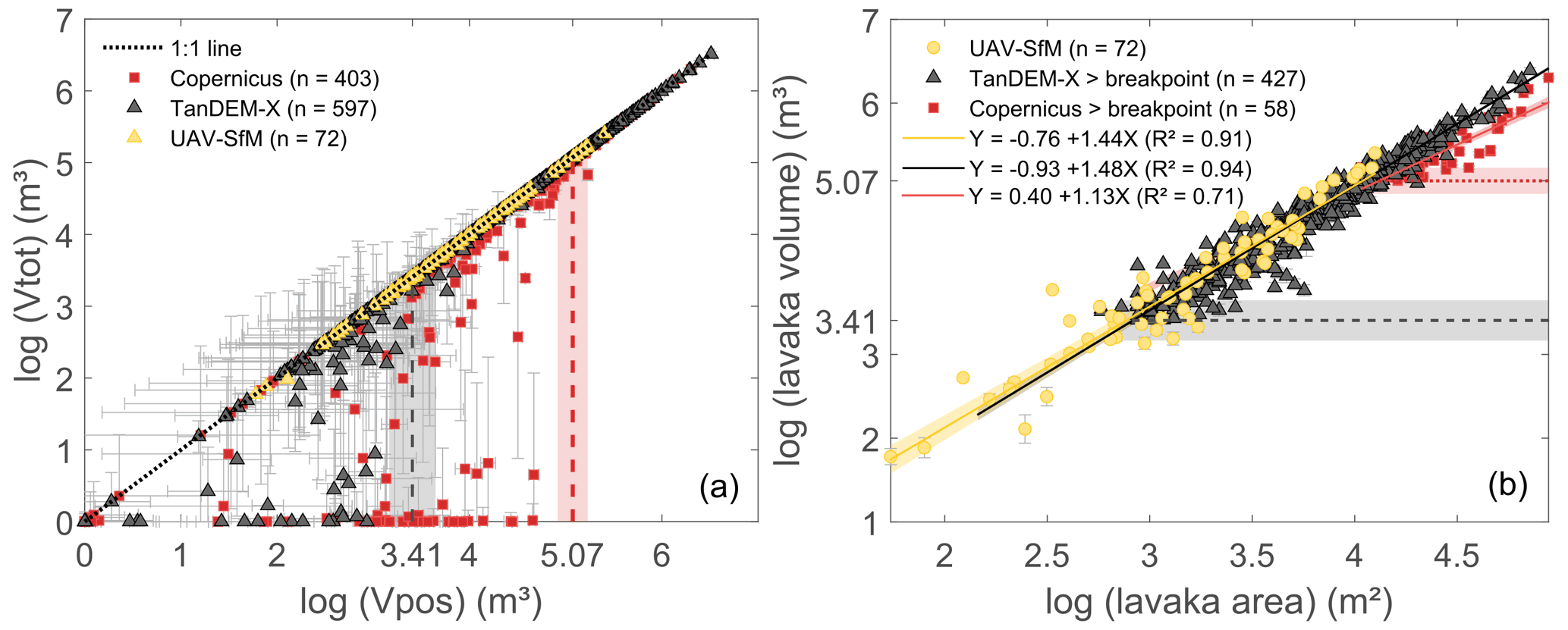
Figure 5Breakpoint analysis and final area–volume relationships. (a) The breakpoint is identified as the point where the RMSE from the 1:1 line of the log-transformed positive (Vpos) and total (Vtot) volumes is smaller than 1 %. The identified breakpoint is located at log (Vpos) = 3.41 ± 0.24 m3 for TanDEM-X and at 5.07 ± 0.16 m3 for Copernicus. (b) Linear area–volume relationships fitted through the log-transformed lavaka area and volume data for the full UAV-SfM dataset and for the TanDEM-X and Copernicus volumes that exceed the identified breakpoints (log (Vpos) > 3.41 ± 0.24 m3 for TanDEM-X and > 5.07 ± 0.16 m3 for Copernicus). Shaded areas indicate the 95 % confidence intervals of the fitted relationships and the standard deviation of the breakpoints. Grey error bars are the standard deviations of the mean calculated volumes representing the total uncertainty (interpolation and relative DEM uncertainty).
While it is clear that both the TanDEM-X DEM and especially the Copernicus DEM are too coarse to accurately predict lavaka volumes for the smallest features, this issue seems to disappear for the larger features. Therefore, we tried to identify the point below which the analysis based on TanDEM-X and Copernicus suffers from errors in volume reconstruction as evidenced by negative volume pixels. This breakpoint was identified as the point where the RMSE from the 1:1 Vpos–Vtot line becomes smaller than 1 %. This breakpoint is for the TanDEM-X DEM located at a positive volume of ca. 2500 ± 1500 m3 and corresponding surface area of ca. 800 ± 250 m2 or 6 ± 2 pixels. For the Copernicus DEM, this point is located at a positive volume of ca. 120 000 ± 45 000 m3, corresponding to a lavaka surface area of 13 000 ± 3500 m2 or 14 ± 5 pixels (Fig. 5a).
In the next step, we established a new area–volume relationship for the TanDEM-X and Copernicus data containing only lavaka volumes larger than their identified breakpoints. Back-transforming the fitted linear log-transformed area–volume relationships results in the following power law lavaka area–volume relationships for the UAV-SfM, TanDEM-X, and Copernicus DEM, where the standard deviation of the back-transformed bias-corrected a and b coefficients are indicated:
For TanDEM-X this results in a close match with the fitted relationship based on the UAV-SfM data, with fitted regression coefficients for TanDEM-X that are within uncertainty of the UAV-SfM coefficients (Fig. 5b and Eqs. 5 and 6). While fitting the relationship only through the data points above the breakpoint results in an area–volume relationship within uncertainty of the ground truth UAV-SfM relationship for the TanDEM-X DEM, this is not the case for the Copernicus DEM. Even when keeping only the data above the identified breakpoint, the fitted area–volume relationship for Copernicus still largely deviates from the UAV-SfM relationship, with a lower scaling coefficient and higher intercept (Fig. 5b, Eqs. 5 and 7). Given the large discrepancy between the UAV-SfM and Copernicus relationship the latter will not be used for further calculations of the volumetric growth and mobilization rates.
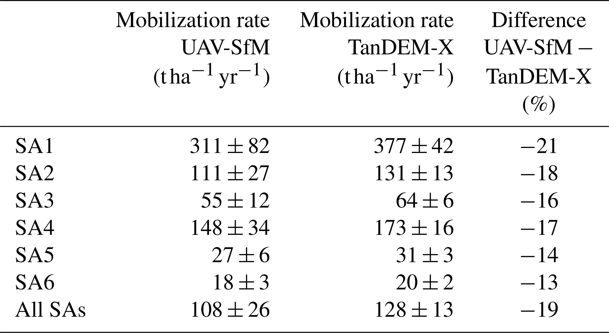
Table 2Lavaka mobilization rates 1949–2010s. Lavaka mobilization rates (in ) obtained by applying the area–volume relationships from the UAV-SfM (Eq. 5) and TanDEM-X (Eq. 6) DEM to the lavaka areas for the longest time period available: 1949–2010s for SA1–5 and 1969–2010s for SA6. Reported values give the median and standard deviation from the 104 Monte Carlo simulations where the uncertainties in the fitted a and b coefficients of the area–volume relationships are accounted for.
3.4 Lavaka volumetric growth and mobilization rates: 1949–2010s
By applying the established area–volume relationships to the historical (1949 for SA1–5 and 1969 for SA6) and current (2010s) lavaka areas (Table S1), volumetric growth rates (VGR in m3 yr−1) could be estimated (Eq. 1). When using the UAV-SfM relationship (Eq. 5), a mean and median growth rate of 1149 ± 275 and 320 ± 56 m3 yr−1 are obtained, respectively. When applying the TanDEM-X relationship (Eq. 6) these values are ca. 15 % higher: 1341 ± 137 and 354 ± 26 m3 yr−1 for the mean and median, respectively. This deviation of 15 % is, however, still within uncertainty of the estimates from the UAV-SfM DEM, which have an uncertainty range of 24 % resulting from the larger uncertainties in the fitted coefficients. This indicates that small variations in the established coefficients can lead to relatively large differences in estimated volumetric growth and mobilization rates.
Volumetric growth rates can be converted to lavaka mobilization rates (LMR, in ) when the bulk density and size of the study areas are taken into account (Eq. 2). Lavaka mobilization rates as derived from the UAV-SfM relationship range between 18 ± 3 and 311 ± 82 in our six study areas (Table 2). LMR values are again estimated to be ca. 13 % to 21 % higher when applying the TanDEM-X relationship (Table 2), resulting in LMR values between 20 ± 2 and 377 ± 42 , which is within uncertainty of the UAV-SfM estimates.
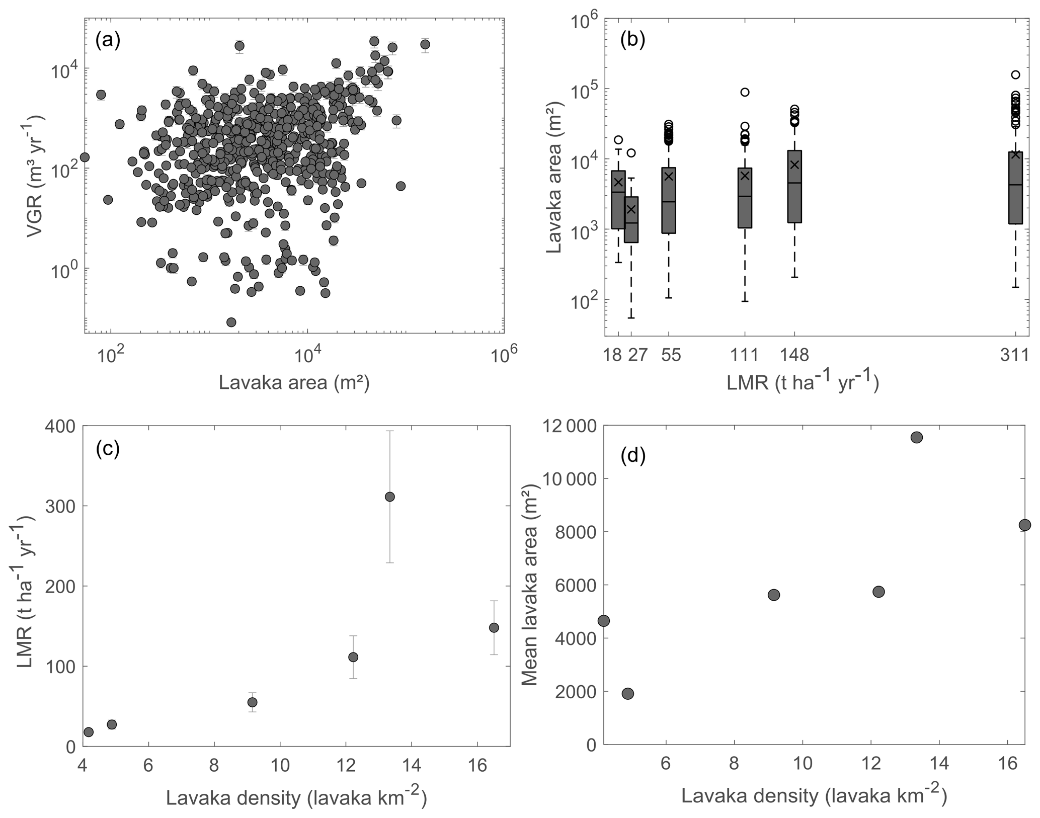
Figure 6Variations in volumetric growth rates and lavaka mobilization rates. (a) Lavaka volumetric growth rates (VGR) are positively related with lavaka area (Spearman correlation coefficient r = 0.27, p = 1 × 10⁻¹⁰). (b) Lavaka mobilization rates (LMR) are higher for study areas with larger lavaka. Mean lavaka areas are indicated by the cross in the boxplot. Higher lavaka mobilization rates are linked to higher lavaka densities (c), which are also positively correlated with lavaka area (d). The variable n indicates the number of observations, and the error bars indicate the standard deviation of the mean LMR as obtained from the Monte Carlo simulations taking into account the uncertainties in the fitted a and b coefficients.
Lavaka mobilization rates seem to be positively correlated with the mean surface area of lavaka in the study area (Fig. 6b). This can be explained by the positive correlation between lavaka area and volumetric growth rate (r = 0.27, p = 1 × 10⁻¹⁰, Fig. 6a): larger lavaka mobilize more material. LMR also increases with increasing lavaka density (Fig. 6c), which is logical but is also partially explained by the positive correlation between lavaka density and mean lavaka surface area (Fig. 6d). The main variations in LMR between our six study areas thus seem to mainly depend on the lavaka density and area distribution. While lavaka presence has been linked to seismic activity (Cox et al., 2010) and is typically associated with slopes ranging between 25 to 30∘ in the Lake Alaotra region (Voarintsoa et al., 2012), differences in surface growth rates could only be poorly linked to other environmental factors: the combined effects of the percentage bare surface area, distance to a stream, and distance to a drainage divide could only explain 18 % of the variation in lavaka growth rates (Brosens et al., 2022).
In order to further evaluate the possible impact of fitting the TanDEM-X relationship to the larger features only (> 800 ± 250 m2), we quantified the share of the total mobilized sediment that is provided by lavaka smaller than 800 ± 250 m2. From the relative cumulative sediment mobilization curves it is apparent that larger lavaka contribute most of the mobilized sediment (Fig. S7). Lavaka that are smaller than the identified threshold contribute 0.2 % of the total mobilized sediment in the study areas with the largest lavaka and up to 2.6 % in the regions with smaller lavaka (Fig. S7). This indicates that the share of smaller lavaka to the total amount of sediment that is mobilized is generally low in our study areas, which therefore reduces the risk of erroneous estimates in cases where these smaller lavaka could not be used to establish the TanDEM-X-based area–volume relationships.
4.1 Interpolation methods and DEM uncertainties
The best interpolation results were obtained when using a regularized spline with tension algorithm (Table 1 and Fig. S5). Bergonse and Reis (2015) concluded that spline interpolation methods result in smaller errors compared to linear methods as they are better adjusted to a gully geomorphic context by allowing curved surfaces in areas with no data, which is not the case for linear interpolation methods. This general conclusion is, however, not necessarily confirmed by our results: while the lowest errors were obtained for the regularized spline with tension algorithm, both other spline algorithms (bilinear and bicubic) performed worse than the linear and TIN interpolation algorithms (Table 1). This might be related to the fact that spline methods are parameterized, where we used the default settings without optimization as an in-depth comparison of different interpolation methods was out of scope for this study.
The UAV-SfM DEM was used as the ground-truth reference in this study. However, like other DEMs, it is constructed from an airborne perspective, where vertical morphologies such as overhanging walls or undercutting or piping features are hidden from the observation point (Frankl et al., 2015). The impact on the estimated volumes should, however, be minimal, as earlier reported volumetric differences are only ca. 2.5 % (Frankl et al., 2015). Volumetric gully measurements from photogrammetric techniques are furthermore reported to suffer from sun- and sight-shadowing, which is especially the case for narrower gullies and might result in inaccuracies in the DEM (Giménez et al., 2009).
The main limitation of the UAV-SfM DEM is the presence of vegetation, making it a digital surface model (DSM) rather than a digital elevation model (DEM). The same is true for the TanDEM-X and Copernicus DEMs, where the relative impact of vegetation on the final elevation will be smaller due to their coarser resolution. The vegetation was not filtered out of any of the data products because most of the land surface in the studied regions is covered with low grassland vegetation. Some trees or bushes are present in the landscape near the hillslope bottoms or inside the stabilizing lavaka (Fig. 1e and f). While the presence of vegetation at the hillslope bottoms might result in a slight overestimation of the interpolated surface, this effect has a minimal impact on the estimated lavaka volumes because at this location lavaka are typically at their narrowest (Wells et al., 1991) (Fig. 1).
A possible caveat when using a fisheye camera for UAV image acquisition is vertical “doming”. However, our flights were carried out with a slightly tilted camera and in a course-aligned way, resulting in oblique images with overlapping areas under a different angle, which is reported to reduce error propagation and doming (James and Robson, 2014). Possible vertical doming could only be verified visually in our case by inspecting the point cloud of flat surfaces in the study area, since no independent GNSS dataset is available. Visual inspection (Fig. S8) and reported vertical deviations less than 0.07 m by Zhang et al. (2019), whose setup was adopted here, confirm that this effect is likely minimal.
4.2 Lavaka volumes and area–volume relationships from varying DEM resolutions
The coarser resolution of the TanDEM-X and Copernicus DEM results in a systematic underestimation of lavaka volumes for all lavaka in the case of Copernicus and for smaller lavaka in the case of TanDEM-X upon direct comparison with the UAV-SfM volumes (Fig. 3a). The first factor that explains this observation is the dependence of the optimal DEM grid resolution on the inherent properties and scale of the geomorphic features under study (Tarolli, 2014; Hengl, 2006; Smith et al., 2019). Theoretically, the minimum size of a landform should be twice the resolution of the DEM, (Theobald, 1989; Frankl et al., 2013), corresponding to 0.16, 576, and 3600 m2 for the UAV-SfM, TanDEM-X, and Copernicus DEM, respectively. Comparing these theoretical minima with the identified breakpoints at 800 ± 250 m2 for the TanDEM-X DEM and 1.3 × 10⁴ ± 3500 m2 for the Copernicus DEM indicates that in practice the aerial DEM resolution has to be 2.4 to 3.8 times the landform size in order to accurately capture it.
While for the TanDEM-X DEM the volumes for features larger than the breakpoint closely match those obtained from the UAV-SfM DEM, this is not the case for the Copernicus DEM (Fig. 5b). This indicates that for the TanDEM-X DEM the largest volumetric errors are contained within the percentage negative volume, as the breakpoint corresponds to the point where the TanDEM-X volumes no longer deviate from the volumes obtained from the UAV-SfM DEM (Fig. 3a). Furthermore, this also resulted in an area–volume relationship for TanDEM-X that is within uncertainty of the UAV-SfM relationship (Fig. 5, Eqs. 5 and 6). A large deviation between the area–volume relationship obtained for the Copernicus DEM and UAV-SfM DEM remained, even when considering only the lavaka located above the breakpoint (Fig. 5b). For the Copernicus DEM the absence of negative volumes in the total volume estimate thus seems to be an insufficient measure to accurately estimate lavaka volumes. This might be related to a second factor that affects estimated volumes, which is the DEM smoothness. The smoothing effect of coarser-resolution DEMs on landscape topographical representation is known to result in a reduced ability to capture more complex topography and geomorphic features (Thompson et al., 2001; Wechsler, 2007; Tarolli, 2014; Hengl, 2006). The underestimation of eroded volumes when coarser-resolution DEMs are used was also reported by Claessens et al. (2005), who found that the highest landslide erosion and deposition volumes were estimated for the highest-resolution DEM and systematically decreased when reducing the DEM resolution. This effect was attributed to the more detailed landscape representation for higher-resolution DEMs.
Our results therefore indicate that for the TanDEM-X DEM our Vpos-Vtot breakpoint method allows us to exclude lavaka that suffer from evident volume reconstruction errors in an objective way. This method can furthermore be applied to regions where no sub-meter-resolution DEMs are available for comparison, as the breakpoint can be determined from the difference between Vtot and Vpos using the coarser-resolution DEM. However, our results also show that the 30 m resolution Copernicus DEM is too coarse and filters out too many topographic details to accurately calculate volumes of erosional features at the lavaka scale (100–105 m2) as large volume underestimations remain even when considering only the largest features (Figs. 3c and 5b).
While coarser-resolution DEMs result in lower volume estimates, volumetric growth and lavaka mobilization rates estimated from the TanDEM-X area–volume relationship are 13 % to 21 % higher than those obtained from the UAV-SfM area–volume relationship (Table 2). From the area–volume graph (Fig. 5b) it can be seen that TanDEM-X slightly underestimates the volumes of lavaka located just above the breakpoint. This “pulls” the linear regression line down for smaller lavaka, resulting in a slightly higher scaling coefficient for the TanDEM-X area–volume relationship (1.48 ± 0.02) when compared to UAV-SfM (1.44 ± 0.04). This results in lavaka volumes that will be slightly underestimated for the smaller features and overestimated for the larger features. As the largest features account for the majority of the mobilization rates (Fig. S7), the volumetric growth and mobilization rates for the TanDEM-X DEM will be overestimated. Further reducing the maximum RMSE below 1 % for the breakpoint determination could resolve this issue but will set the minimum lavaka area higher, further reducing the number of observations.
Gully volumes are typically linked to gully length as most gullies mainly lengthen when they grow (Frankl et al., 2013; Vanmaercke et al., 2021). Lavaka, in contrast, deepen, widen and lengthen when they grow, which is why we link lavaka volume with area instead of length. While this does not allow direct comparison with other relationships obtained for gullies, previous studies reported that length–volume relationships are region-specific (Frankl et al., 2013). Applying the observed relationship outside of the Lake Alaotra region should therefore be done with care and might require validation. While the processes of landslide and lavaka erosion are entirely different, the obtained scaling coefficient a of 1.44 ± 0.04 indicates that for a given area lavaka volumes will be similar to those of deep landslides, which typically have an a between 1.3 and 1.6 (Larsen et al., 2010).
In a typical pattern of development, lavaka start as raw patches that evolve to step-like headscarps, grow into deep inverse teardrop-shaped gullies and finally become longer, broader, gentler, and partly filled concavities when stabilizing (Wells et al., 1991). Upon stabilization lavaka will partially fill in, reducing the volume. Not all lavaka will stabilize at the same size or grow in the same way. This will likely be one of the main factors explaining the remaining 6 % to 9 % of variation in lavaka volume that cannot be explained by the area (R2 = 0.94 and 0.91 for TanDEM-X and UAV-SfM, respectively) (Fig. 5).
4.3 Lavaka mobilization rates put into perspective
Our calculated lavaka mobilization rates from direct lavaka growth observations over the period 1949–2010s (ca. 70 years) range between 18 ± 3 and 311 ± 82 for six ca. 10 km2 study areas in the Lake Alaotra region with an overall average of 108 ± 26 (Table 2). It should, however, be noted that our highest reported LMRs of 311 ± 82 and 148 ± 34 correspond to areas characterized by large lavaka and high lavaka densities (13 and 17 lavaka per square kilometer, Table S1, Fig. 6b). These lavaka densities are higher than the reported average of six lavaka per square kilometer for the southern part of the Lake Alaotra catchment (Voarintsoa et al., 2012). We therefore argue that these highest values should be perceived as maximum rates, where the rates of 18–53 obtained for regions with lower lavaka densities (SA 3, 5, and 6, Table S1) will be more representative for the wider Lake Alaotra region (Table 2).
Only limited local data are available that can be used to compare these estimates. A sedimentation rate of 20 was obtained by Mietton et al. (2006) for the dammed Lake Bevava, which is located in the southeastern part of the Lake Alaotra catchment, over the period 1987–2005. Lake Bevava has a catchment area of 58 km2 with a lavaka density of eight lavaka per square kilometer (Mietton et al., 2006). The reported recent lake sedimentation rate of 20 is less than half of our calculated lavaka mobilization rate of 53 ± 19 for SA3, which has a comparable lavaka density of nine lavaka per square kilometer (Fig. 6c, Tables S1 and 2). While both estimates are of the same order of magnitude, this suggests that a considerable proportion (more than 50 %) of the mobilized sediment will likely be trapped close to the lavaka and not reach the rivers or lake.
Next to these recent short-term sedimentation rates, long-term catchment-wide erosion rates obtained from 10Be measurements have been reported for the central Malagasy highlands. These 10Be erosion rates integrate over a timescale of thousands to hundreds of thousands of years and represent long-term averages. Reported long-term 10Be erosion rates range from 0.16 to 0.54 , with the highest rates for the catchments with higher lavaka densities (max. six lavaka per square kilometer, Cox et al., 2009). Ideally these long-term rates are compared with current sediment yields or sedimentation data (Bartley et al., 2015; Vanacker et al., 2007), as a considerable fraction of the sediment likely never reaches the rivers or lakes. However, the offset of 2 orders of magnitude between long-term 10Be erosion rates and current lavaka mobilization rates and Lake Bevava sedimentation rates suggests that lavaka erosion has increased over recent time periods in the Lake Alaotra region. This was also concluded by Brosens et al. (2022), where a 10-fold increase in floodplain sedimentation rates was observed over the past 1000 years, which was linked to a recent increase in lavaka activity brought about by increasing environmental pressure due to growing human and cattle populations (Joseph et al., 2021).
Globally reported volumetric gully erosion rates range between 0.0002 and 47 430 m3 yr−1, with mean and median values of 359 and 2.2 m3 yr−1 (Vanmaercke et al., 2016). Our mean and median estimated volumetric growth rates of 1149 ± 275 and 320 ± 56 m3 yr−1 are at least 3 times higher than these global averages, indicating that lavaka erosion in the Lake Alaotra catchment is occurring at above-average gully erosion rates. These reported volumetric gully growth rates correspond to global mean and median aerial gully growth rates of 3.1 and 131 m2 yr−1 (Vanmaercke et al., 2016), whereas the mean and median aerial lavaka growth rates for our lavaka dataset are 22 and 11 m2 yr−1 (Brosens et al., 2022). This indicates that while volumetric lavaka growth rates are higher than the global averages, their change in aerial extent is below average. This is caused by the specific morphology of lavaka, which are much deeper than average gullies with estimated mean and median depths for our dataset of 23 and 19 m based on the calculated volumes and areas, whereas this is only 2.1 and 1.3 m for the global dataset (Vanmaercke et al., 2016).
Lavaka volumes were estimated as the difference between the current and interpolated pre-erosion surface for three DEMs with different spatial resolutions: UAV-SfM (0.2 m), TanDEM-X (12 m), and Copernicus (30 m). Volumes estimated from TanDEM-X are similar to those obtained from the UAV-SfM DEM for the larger features. Using the Copernicus DEM results in strong volume underestimations, even for the largest features. This indicates that the Copernicus DEM is not suitable to estimate erosion volumes for geomorphic features at the lavaka scale (100–105 m2), due to a smoothing effect that means that complex topography and smaller geomorphic features cannot be accurately captured by its coarser resolution. TanDEM-X can be used for volume estimations but shows a tendency to underestimate volumes for small lavaka. An area–volume relationship, necessary for large-scale and past volume assessments, can be established using TanDEM-X or UAV-SfM data. However, developing a robust relationship based on the TanDEM-X data requires that observations for which the relative reconstruction error is too large are eliminated from the dataset. In this paper, we proposed and tested a method to identify a cut-off point below which volume estimations are clearly affected by processing errors as evidenced by negative volume estimates. This breakpoint is located at a lavaka volume of ca. 2500 ± 1500 m3, corresponding to an area of ca. 800 ± 250 m2. The proposed objective filtering to eliminate erroneous volumes in the TanDEM-X estimates resulted in deviations in lavaka growth rates and mobilization rates that are ca. 13 % to 21 % higher compared to the respective UAV-SfM estimates but fall within the uncertainty boundaries of the latter. Our results thus indicate that the TanDEM-X DEM can be used to establish accurate area–volume relationships for erosional features at the lavaka scale when applying the breakpoint method. As this method does not depend on direct comparison with higher-resolution DEMs, it can be applied to regions where only TanDEM-X is available. Over the period 1949–2010s, a mean and median lavaka volumetric growth rate of 1149 ± 275 and 320 ± 56 m3 yr−1 and lavaka mobilization rates varying between 18 ± 3 and 311 ± 82 were obtained. While our highest lavaka mobilization rates are likely limited to the most lavaka-dense regions, our lower estimates are consistent with reservoir siltation rates, placing the current average lavaka mobilization rate for the Lake Alaotra region at 20–50 . These rates are furthermore 2 orders of magnitude higher than earlier reported long-term erosion rates, suggesting a recent increase in lavaka erosion intensity in the Lake Alaotra region.
All 12 m TanDEM-X files (DEM and auxiliary files) were provided by DLR under a scientific-use user license. The Copernicus DEM is freely available through ESA's data portal. WorldView-2 imagery was available as a base layer in ArcMap software from Esri. All data from the lavaka dataset can be found at https://doi.org/10.6084/m9.figshare.c.5236322.v1 (Brosens, 2020). The PyQGIS code used to extract the lavaka volumes, an example dataset, and an excel table with all the calculated volumes and VGRs can be found at https://doi.org/10.5281/zenodo.5768418 (Brosens, 2021).
The supplement related to this article is available online at: https://doi.org/10.5194/esurf-10-209-2022-supplement.
GG and SB acquired funding for the project and designed the study together with LJ, BC, TRaz, and TRaf, and the main supervision was provided by LJ. Obtaining the necessary drone permits and flights was successful due to the mutual efforts of LJ, BC, VFR, LB and EAJ. EAJ was the remote pilot of the UAV and co-developed the UAV-PPK-SfM method used in this paper. LB analyzed the data and wrote the manuscript with input from all authors.
The contact author has declared that neither they nor their co-authors have any competing interests.
Publisher's note: Copernicus Publications remains neutral with regard to jurisdictional claims in published maps and institutional affiliations.
This research would not have been possible without the help of our local partners at Laboratoire des RadioIsotopes and the local authorities of the Ambatondrazaka and Amparafaravola district and the authorization from the Aviation Civil de Madagascar to fly the UAV over their territories. Kristof Van Oost's expertise was crucial for obtaining high-quality UAV DEMs. Ny Riavo Voarintsoa, Rónadh Cox, and Steven Bouillon are wholeheartedly thanked for their insights and inspiring discussions on this topic. This research is part of the MaLESA project funded by a KU Leuven Special Research Fund grant (An integrated approach for assessing environmental changes in soil-covered landscapes: the case of Madagascar). We are very grateful for the constructive feedback provided by Benjamin Purinton, Amaury Frankl, and Rónadh Cox, which has drastically improved the methodological rigour and quality of this paper.
This research has been supported by YouReCa, the Fonds Wetenschappelijk Onderzoek (grant nos. 11B6921N, 12Z6518N, V436719N, and V436319N).
This paper was edited by Giulia Sofia and reviewed by Amaury Frankl and Benjamin Purinton.
AIRBUS: Copernicus Digital Elevation Model Product Handbook, Tech. rep., AIRBUS Defence and Space GmbH, https://spacedata.copernicus.eu/documents/20126/0/GEO1988-CopernicusDEM-SPE-002_ProductHandbook_I1.00.pdf (last access: 11 March 2022), 2020a.
AIRBUS: Copernicus Digital Elevation Model Validation Report, Tech. rep., AIRBUS Defence and Space GmbH, https://spacedata.copernicus.eu/documents/20126/0/GEO1988-CopernicusDEM-RP-001_ValidationReport_V1.0.pdf (last access: 11 March 2022), 2020b.
Bangen, S. G., Wheaton, J. M., Bouwes, N., Bouwes, B., and Jordan, C.: A methodological intercomparison of topographic survey techniques for characterizing wadeable streams and rivers, Geomorphology, 206, 343–361, https://doi.org/10.1016/j.geomorph.2013.10.010, 2014.
Bartley, R., Croke, J., Bainbridge, Z. T., Austin, J. M., and Kuhnert, P. M.: Combining contemporary and long-term erosion rates to target erosion hot-spots in the Great Barrier Reef, Australia, Anthropocene, 10, 1–12, https://doi.org/10.1016/j.ancene.2015.08.002, 2015.
Bergonse, R. and Reis, E.: Reconstructing pre-erosion topography using spatial interpolation techniques: A validation-based approach, J. Geogr. Sci., 25, 196–210, https://doi.org/10.1007/s11442-015-1162-2, 2015.
Bourgeat, F.: Sols sur socle ancien a Madagascar. Types de différenciation et interprétation chronologique au cours du quaternaire., Tech. rep., ORSTROM, Paris, 1972.
Broeckx, J., Maertens, M., Isabirye, M., Vanmaercke, M., Namazzi, B., Deckers, J., Tamale, J., Jacobs, L., Thiery, W., Kervyn, M., Vranken, L., and Poesen, J.: Landslide susceptibility and mobilization rates in the Mount Elgon region, Uganda, Landslides, 16, 571–584, https://doi.org/10.1007/s10346-018-1085-y, 2019.
Brosens, L.: Data for: “Is there an environmental crisis in Madagascar's highlands? Insights from lavaka demographics”, figshare Collection [data set], https://doi.org/10.6084/m9.figshare.c.5236322.v1, 2020.
Brosens, L.: LBrosens/LavakaVolumes: LavakaVolumes-v2 (v2.0), Zenodo [code], https://doi.org/10.5281/zenodo.5768418, 2021.
Brosens, L., Broothaerts, N., Campforts, B., Jacobs, L., Razanamahandry, V. F., Van Moerbeke, Q., Bouillon, S., Razafimbelo, T., Rafolisy, T., and Govers, G.: Under pressure: Rapid lavaka erosion and floodplain sedimentation in central Madagascar, Sci. Total Environ., 806, 150483, https://doi.org/10.1016/j.scitotenv.2021.150483, 2022.
Brovelli, M. A., Cannata, M., and Longoni, U. M.: LIDAR Data Filtering and DTM Interpolation Within GRASS, T. GIS, 8, 155–174, https://doi.org/10.1111/j.1467-9671.2004.00173.x, 2004.
Castillo, C., Pérez, R., James, M. R., Quinton, J. N., Taguas, E. V., and Gómez, J. A.: Comparing the Accuracy of Several Field Methods for Measuring Gully Erosion, Soil Sci. Soc. Am. J., 76, 1319–1332, https://doi.org/10.2136/sssaj2011.0390, 2012.
Claessens, L., Heuvelink, G. B. M., Schoorl, J. M., and Veldkamp, A.: DEM resolution effects on shallow landslide hazard and soil redistribution modelling, Earth Surf. Proc. Land., 30, 461–477, https://doi.org/10.1002/esp.1155, 2005.
Clapuyt, F., Vanacker, V., and Van Oost, K.: Reproducibility of UAV-based earth topography reconstructions based on Structure-from-Motion algorithms, Geomorphology, 260, 4–15, https://doi.org/10.1016/j.geomorph.2015.05.011, 2016.
Cook, K. L.: An evaluation of the effectiveness of low-cost UAVs and structure from motion for geomorphic change detection, Geomorphology, 278, 195–208, https://doi.org/10.1016/j.geomorph.2016.11.009, 2017.
Cox, R., Bierman, P., Jungers, M. C., and Rakotondrazafy, A. F. M.: Erosion Rates and Sediment Sources in Madagascar Inferred from 10Be Analysis of Lavaka, Slope, and River Sediment, J. Geol., 117, 363–376, https://doi.org/10.1086/598945, 2009.
Cox, R., Zentner, D. B., Rakotondrazafy, A. F. M., and Rasoazanamparany, C. F.: Shakedown in Madagascar: Occurrence of lavakas (erosional gullies) associated with seismic activity, Geology, 38, 179–182, https://doi.org/10.1130/G30670.1, 2010.
Crawford, C. G.: Estimation of suspended-sediment rating curves and mean suspended-sediment loads, J. Hydrol., 129, 331–348, https://doi.org/10.1016/0022-1694(91)90057-O, 1991.
Eustace, A., Pringle, M., and Witte, C.: Innovations in Remote Sensing and Photogrammetry, Lecture Notes in Geoinformation and Cartography, Springer Berlin Heidelberg, Berlin, Heidelberg, https://doi.org/10.1007/978-3-540-93962-7, 2009.
Evans, M. and Lindsay, J.: High resolution quantification of gully erosion in upland peatlands at the landscape scale, Earth Surf. Proc. Land., 35, 876–886, https://doi.org/10.1002/esp.1918, 2010.
Ferguson, R. I.: River Loads Underestimated by Rating Curves, Water Resour. Res., 22, 74–76, https://doi.org/10.1029/WR022i001p00074, 1986.
Fisher, G. B., Amos, C. B., Bookhagen, B., Burbank, D. W., and Godard, V.: Channel widths, landslides, faults, and beyond: The new world order of high-spatial resolution Google Earth imagery in the study of earth surface processes, in: Google Earth and Virtual Visualizations in Geoscience Education and Research, vol. 492, edited by: Whitmeyer, S. J. and Manduca, C. A., Geological Society of America, 1–22, https://doi.org/10.1130/2012.2492(01), 2012.
Frankl, A., Poesen, J., Scholiers, N., Jacob, M., Haile, M., Deckers, J., and Nyssen, J.: Factors controlling the morphology and volume (V)-length (L) relations of permanent gullies in the northern Ethiopian Highlands, Earth Surf. Proc. Land., 38, 1672–1684, https://doi.org/10.1002/esp.3405, 2013.
Frankl, A., Stal, C., Abraha, A., Nyssen, J., Rieke-Zapp, D., De Wulf, A., and Poesen, J.: Detailed recording of gully morphology in 3D through image-based modelling, Catena, 127, 92–101, https://doi.org/10.1016/j.catena.2014.12.016, 2015.
Frankl, A., Nyssen, J., Vanmaercke, M., and Poesen, J.: Gully prevention and control: Techniques, failures and effectiveness, Earth Surf. Proc. Land., 46, 220–238, https://doi.org/10.1002/esp.5033, 2021.
Frees, E. W. and Valdez, E. A.: Understanding Relationships Using Copulas, North American Actuarial Journal, 2, 1–25, https://doi.org/10.1080/10920277.1998.10595667, 1998.
GDAL: GDAL grid documentation, https://gdal.org/programs/gdal_grid.html, last access: 7 April 2021.
Giménez, R., Marzolff, I., Campo, M. A., Seeger, M., Ries, J. B., Casalí, J., and Álvarez-Mozos, J.: Accuracy of high-resolution photogrammetric measurements of gullies with contrasting morphology, Earth Surf. Proc. Land., 34, 1915–1926, https://doi.org/10.1002/esp.1868, 2009.
GRASS: v.surf.rst, https://grass.osgeo.org/grass78/manuals/v.surf.rst.html (last access: 7 April 2021), 2003.
GRASS: v.surf.bspline, https://grass.osgeo.org/grass80/manuals/v.surf.bspline.html, last access: 7 April 2021.
Grohmann, C. H.: Evaluation of TanDEM-X DEMs on selected Brazilian sites: Comparison with SRTM, ASTER GDEM and ALOS AW3D30, Remote Sens. Environ., 212, 121–133, https://doi.org/10.1016/j.rse.2018.04.043, 2018.
Guth, P. L. and Geoffroy, T. M.: LiDAR point cloud and ICESat-2 evaluation of 1 second global digital elevation models: Copernicus wins, T. GIS, 25, 2245–2261, https://doi.org/10.1111/tgis.12825, 2021.
Guzzetti, F., Ardizzone, F., Cardinali, M., Rossi, M., and Valigi, D.: Landslide volumes and landslide mobilization rates in Umbria, central Italy, Earth Planet. Sc. Lett., 279, 222–229, https://doi.org/10.1016/j.epsl.2009.01.005, 2009.
Guzzetti, F., Mondini, A. C., Cardinali, M., Fiorucci, F., Santangelo, M., and Chang, K.-T.: Landslide inventory maps: New tools for an old problem, Earth-Sci. Rev., 112, 42–66, https://doi.org/10.1016/j.earscirev.2012.02.001, 2012.
Hengl, T.: Finding the right pixel size, Comput. Geosci., 32, 1283–1298, https://doi.org/10.1016/j.cageo.2005.11.008, 2006.
Hovius, N., Stark, C. P., and Allen, P. A.: Sediment flux from a mountain belt derived by landslide mapping, Geology, 25, 231, https://doi.org/10.1130/0091-7613(1997)025<0231:SFFAMB>2.3.CO;2, 1997.
James, M. R. and Robson, S.: Mitigating systematic error in topographic models derived from UAV and ground-based image networks, Earth Surf. Proc. Land., 39, 1413–1420, https://doi.org/10.1002/esp.3609, 2014.
Joseph, G. S., Rakotoarivelo, A. R., and Seymour, C. L.: How expansive were Malagasy Central Highland forests, ericoids, woodlands and grasslands? A multidisciplinary approach to a conservation conundrum, Biol. Conserv., 261, 109282, https://doi.org/10.1016/j.biocon.2021.109282, 2021.
Kompani-Zare, M., Soufi, M., Hamzehzarghani, H., and Dehghani, M.: The effect of some watershed, soil characteristics and morphometric factors on the relationship between the gully volume and length in Fars Province, Iran, Catena, 86, 150–159, https://doi.org/10.1016/j.catena.2011.03.008, 2011.
Krieger, G., Moreira, A., Fiedler, H., Hajnsek, I., Werner, M., Younis, M., and Zink, M.: TanDEM-X: A Satellite Formation for High-Resolution SAR Interferometry, IEEE T. Geosci. Remote, 45, 3317–3341, https://doi.org/10.1109/TGRS.2007.900693, 2007.
Krieger, G., Zink, M., Bachmann, M., Bräutigam, B., Schulze, D., Martone, M., Rizzoli, P., Steinbrecher, U., Walter Antony, J., De Zan, F., Hajnsek, I., Papathanassiou, K., Kugler, F., Rodriguez Cassola, M., Younis, M., Baumgartner, S., López-Dekker, P., Prats, P., and Moreira, A.: TanDEM-X: A radar interferometer with two formation-flying satellites, Acta Astronaut., 89, 83–98, https://doi.org/10.1016/j.actaastro.2013.03.008, 2013.
Kusky, T. M., Toraman, E., Raharimahefa, T., and Rasoazanamparany, C.: Active tectonics of the Alaotra–Ankay Graben System, Madagascar: Possible extension of Somalian–African diffusive plate boundary?, Gondwana Res., 18, 274–294, https://doi.org/10.1016/j.gr.2010.02.003, 2010.
Lammers, P. L., Richter, T., Waeber, P. O., and Mantilla-Contreras, J.: Lake Alaotra wetlands: how long can Madagascar's most important rice and fish production region withstand the anthropogenic pressure?, Madagascar Conserv. Dev., 10, 116–127, https://doi.org/10.4314/mcd.v10i3.4, 2015.
Larsen, I. J., Montgomery, D. R., and Korup, O.: Landslide erosion controlled by hillslope material, Nat. Geosci., 3, 247–251, https://doi.org/10.1038/ngeo776, 2010.
Liu, K., Ding, H., Tang, G., Na, J., Huang, X., Xue, Z., Yang, X., and Li, F.: Detection of Catchment-Scale Gully-Affected Areas Using Unmanned Aerial Vehicle (UAV) on the Chinese Loess Plateau, ISPRS Int. Geo-Inf., 5, 238, https://doi.org/10.3390/ijgi5120238, 2016.
Malamud, B. D., Turcotte, D. L., Guzzetti, F., and Reichenbach, P.: Landslide inventories and their statistical properties, Earth Surf. Proc. Land., 29, 687–711, https://doi.org/10.1002/esp.1064, 2004.
Marešová, J., Gdulová, K., Pracná, P., Moravec, D., Gábor, L., Prošek, J., Barták, V., and Moudrý, V.: Applicability of Data Acquisition Characteristics to the Identification of Local Artefacts in Global Digital Elevation Models: Comparison of the Copernicus and TanDEM-X DEMs, Remote Sens.-Basel, 13, 3931, https://doi.org/10.3390/rs13193931, 2021.
Mietton, M., Leprun, J.-C., Andrianaivoarivony, R., Dubar, M., Beiner, M., Erismann, J., Bonnier, F., Grisorio, E., Rafanomezana, J.-P., and Grandjean, P.: Ancienneté et vitesse d'érosion des lavaka à Madagascar, Tech. rep., in: Erosion et gestion conservatoire de l'eau et de la fertilité des sols: actes des journées scientifiques du réseau Erosion et GCES de l'AUF, edited by: Georges, R. S. S., De Noni, G., and Roose, E., https://www.documentation.ird.fr/hor/fdi:010037411 (last access: 11 March 2022), 2006.
Mietton, M., Gunnell, Y., Nicoud, G., Ferry, L., Razafimahefa, R., and Grandjean, P.: 'Lake' Alaotra, Madagascar: A late Quaternary wetland regulated by the tectonic regime, Catena, 165, 22–41, https://doi.org/10.1016/j.catena.2018.01.021, 2018.
Milliman, J. D. and Farnsworth, K. L.: River Discharge to the Coastal Ocean, Cambridge University Press, Cambridge, https://doi.org/10.1017/CBO9780511781247, 2011.
Mitášová, H. and Mitáš, L.: Interpolation by regularized spline with tension: I. Theory and implementation, Math. Geol., 25, 641–655, https://doi.org/10.1007/BF00893171, 1993.
Montgomery, D. R.: Soil erosion and agricultural sustainability, P. Natl. Acad. Sci. USA, 104, 13268–13272, https://doi.org/10.1073/pnas.0611508104, 2007.
Mudd, S. M.: Topographic data from satellites, in: Developments in Earth Surface Processes, vol. 23, edited by: Tarolli, P. and Mudd, S. M., Elsevier B. V., 91–128, https://doi.org/10.1016/B978-0-444-64177-9.00004-7, 2020.
Niculiţă, M., Mărgărint, M. C., and Tarolli, P.: Using UAV and LiDAR data for gully geomorphic changes monitoring, in: Developments in Earth Surface Processes, vol. 23, pp. 271–315, Elsevier, https://doi.org/10.1016/B978-0-444-64177-9.00010-2, 2020.
Passalacqua, P., Belmont, P., Staley, D. M., Simley, J. D., Arrowsmith, J. R., Bode, C. A., Crosby, C., DeLong, S. B., Glenn, N. F., Kelly, S. A., Lague, D., Sangireddy, H., Schaffrath, K., Tarboton, D. G., Wasklewicz, T., and Wheaton, J. M.: Analyzing high resolution topography for advancing the understanding of mass and energy transfer through landscapes: A review, Earth-Sci. Rev., 148, 174–193, https://doi.org/10.1016/j.earscirev.2015.05.012, 2015.
Perroy, R. L., Bookhagen, B., Asner, G. P., and Chadwick, O. A.: Comparison of gully erosion estimates using airborne and ground-based LiDAR on Santa Cruz Island, California, Geomorphology, 118, 288–300, https://doi.org/10.1016/j.geomorph.2010.01.009, 2010.
Poesen, J., Nachtergaele, J., Verstraeten, G., and Valentin, C.: Gully erosion and environmental change: importance and research needs, Catena, 50, 91–133, https://doi.org/10.1016/S0341-8162(02)00143-1, 2003.
Purinton, B. and Bookhagen, B.: Validation of digital elevation models (DEMs) and comparison of geomorphic metrics on the southern Central Andean Plateau, Earth Surf. Dynam., 5, 211–237, https://doi.org/10.5194/esurf-5-211-2017, 2017.
Purinton, B. and Bookhagen, B.: Beyond Vertical Point Accuracy: Assessing Inter-pixel Consistency in 30 m Global DEMs for the Arid Central Andes, Front. Earth Sci., 9, 1–24, https://doi.org/10.3389/feart.2021.758606, 2021.
QGIS: TIN interpolation, https://docs.qgis.org/3.10/en/docs/user_manual/processing_algs/qgis/interpolation.html#tin-interpolation (last access: 7 April 2021), 2020.
Randrianarijaona, P.: The Erosion of Madagascar, Ambio, 12, 308–311, 1983.
Riquier, J. and Segalen, P.: Notice sur la Pedologique du Lac Alaotra, Tech. rep., Mémoires de l'Institut Scientifique de Madagascar, Série D: Sciences de la Terre (MDG), https://www.documentation.ird.fr/hor/fdi:12926 (last access: 11 March 2022), 1949.
Rizzoli, P., Martone, M., Gonzalez, C., Wecklich, C., Borla Tridon, D., Bräutigam, B., Bachmann, M., Schulze, D., Fritz, T., Huber, M., Wessel, B., Krieger, G., Zink, M., and Moreira, A.: Generation and performance assessment of the global TanDEM-X digital elevation model, ISPRS J. Photogramm., 132, 119–139, https://doi.org/10.1016/j.isprsjprs.2017.08.008, 2017.
Shapiro, S. S. and Wilk, M. B.: An Analysis of Variance Test for Normality (Complete Samples), Tech. Rep. 3, https://www.jstor.org/stable/2333709 (last access: 11 March 2022), 1965.
Smith, T., Rheinwalt, A., and Bookhagen, B.: Determining the optimal grid resolution for topographic analysis on an airborne lidar dataset, Earth Surf. Dynam., 7, 475–489, https://doi.org/10.5194/esurf-7-475-2019, 2019.
Stott, E., Williams, R. D., and Hoey, T. B.: Ground Control Point Distribution for Accurate Kilometre-Scale Topographic Mapping Using an RTK-GNSS Unmanned Aerial Vehicle and SfM Photogrammetry, Drones, 4, 55, https://doi.org/10.3390/drones4030055, 2020.
Taddia, Y., Stecchi, F., and Pellegrinelli, A.: Coastal Mapping Using DJI Phantom 4 RTK in Post-Processing Kinematic Mode, Drones, 4, 9, https://doi.org/10.3390/drones4020009, 2020.
Takasu, T. and Yasuda, A.: Development of the low-cost RTK-GPS receiver with an open source program package RTKLIB, in: International Symposium on GPS/GNSS, 4–6 November 2009, Jeju, Korea, http://gpspp.sakura.ne.jp/paper2005/isgps_2009_rtklib_revA.pdf (last access: 11 March 2022), 2009.
Tarolli, P.: High-resolution topography for understanding Earth surface processes: Opportunities and challenges, Geomorphology, 216, 295–312, https://doi.org/10.1016/j.geomorph.2014.03.008, 2014.
Theobald, D. M.: Accuracy and bias issues in surface representation, in: The Accuracy Of Spatial Databases, 1st edn., edited by: Goodchild, M. F. and Gopal, S., CRC Press, London, 77–82, https://doi.org/10.1201/b12612-20, 1989.
Thompson, J. A., Bell, J. C., and Butler, C. A.: Digital elevation model resolution: effects on terrain attribute calculation and quantitative soil-landscape modeling, Geoderma, 100, 67–89, https://doi.org/10.1016/S0016-7061(00)00081-1, 2001.
Vallejo Orti, M., Negussie, K., Corral-Pazos-de Provens, E., Höfle, B., and Bubenzer, O.: Comparison of Three Algorithms for the Evaluation of TanDEM-X Data for Gully Detection in Krumhuk Farm (Namibia), Remote Sens.-Basel, 11, 1327, https://doi.org/10.3390/rs11111327, 2019.
Vanacker, V., von Blanckenburg, F., Govers, G., Molina, A., Poesen, J., Deckers, J., and Kubik, P.: Restoring dense vegetation can slow mountain erosion to near natural benchmark levels, Geology, 35, 303, https://doi.org/10.1130/G23109A.1, 2007.
Vanmaercke, M., Poesen, J., Van Mele, B., Demuzere, M., Bruynseels, A., Golosov, V., Bezerra, J. F. R., Bolysov, S., Dvinskih, A., Frankl, A., Fuseina, Y., Guerra, A. J. T., Haregeweyn, N., Ionita, I., Makanzu Imwangana, F., Moeyersons, J., Moshe, I., Nazari Samani, A., Niacsu, L., Nyssen, J., Otsuki, Y., Radoane, M., Rysin, I., Ryzhov, Y. V., and Yermolaev, O.: How fast do gully headcuts retreat?, Earth-Sci. Rev., 154, 336–355, https://doi.org/10.1016/j.earscirev.2016.01.009, 2016.
Vanmaercke, M., Panagos, P., Vanwalleghem, T., Hayas, A., Foerster, S., Borrelli, P., Rossi, M., Torri, D., Casali, J., Borselli, L., Vigiak, O., Maerker, M., Haregeweyn, N., De Geeter, S., Zgłobicki, W., Bielders, C., Cerdà, A., Conoscenti, C., de Figueiredo, T., Evans, B., Golosov, V., Ionita, I., Karydas, C., Kertész, A., Krása, J., Le Bouteiller, C., Radoane, M., Ristić, R., Rousseva, S., Stankoviansky, M., Stolte, J., Stolz, C., Bartley, R., Wilkinson, S., Jarihani, B., and Poesen, J.: Measuring, modelling and managing gully erosion at large scales: A state of the art, Earth-Sci. Rev., 218, 103637, https://doi.org/10.1016/j.earscirev.2021.103637, 2021.
Voarintsoa, N. R. G., Cox, R., Razanatseheno, M. O. M., and Rakotondrazafy, A. F. M.: Relation between bedrock geology, topography and lavaka distribution in Madagascar, S. Afr. J. Geol., 115, 225–250, https://doi.org/10.2113/gssajg.115.225, 2012.
Wechsler, S. P.: Uncertainties associated with digital elevation models for hydrologic applications: a review, Hydrol. Earth Syst. Sci., 11, 1481–1500, https://doi.org/10.5194/hess-11-1481-2007, 2007.
Wells, N. A. and Andriamihaja, B.: The initiation and growth of gullies in Madagascar: are humans to blame?, Geomorphology, 8, 1–46, https://doi.org/10.1016/0169-555X(93)90002-J, 1993.
Wells, N. A., Andriamihaja, B., and Rakotovololona, H. F. S.: Patterns of development of lavaka, Madagascar's unusual gullies, Earth Surf. Proc. Land., 16, 189–206, https://doi.org/10.1002/esp.3290160302, 1991.
Wessel, B.: TanDEM-X Ground Segment DEM Products Specification Document, Tech. rep., EOC – Earth Observation Center, https://elib.dlr.de/108014/ (last access: 11 March 2022), 2016.
Wessel, B., Huber, M., Wohlfart, C., Marschalk, U., Kosmann, D., and Roth, A.: Accuracy assessment of the global TanDEM-X Digital Elevation Model with GPS data, ISPRS J. Photogramm., 139, 171–182, https://doi.org/10.1016/j.isprsjprs.2018.02.017, 2018.
Zhang, H., Aldana-Jague, E., Clapuyt, F., Wilken, F., Vanacker, V., and Van Oost, K.: Evaluating the potential of post-processing kinematic (PPK) georeferencing for UAV-based structure- from-motion (SfM) photogrammetry and surface change detection, Earth Surf. Dynam., 7, 807–827, https://doi.org/10.5194/esurf-7-807-2019, 2019.
The requested paper has a corresponding corrigendum published. Please read the corrigendum first before downloading the article.
- Article
(6019 KB) - Full-text XML
- Corrigendum
-
Supplement
(5436 KB) - BibTeX
- EndNote