the Creative Commons Attribution 4.0 License.
the Creative Commons Attribution 4.0 License.
 | 04 Apr 2022
A geomorphic-process-based cellular automata model of colluvial wedge morphology and stratigraphy
Christopher B. DuRoss
Sylvia R. Nicovich
Ryan D. Gold
The development of colluvial wedges at the base of fault scarps following normal-faulting earthquakes serves as a sedimentary record of paleoearthquakes and is thus crucial in assessing seismic hazard. Although there is a large body of observations of colluvial wedge development, connecting this knowledge to the physics of sediment transport can open new frontiers in our understanding. To explore theoretical colluvial wedge evolution, we develop a cellular automata model driven by the production and disturbance (e.g., bioturbative reworking) of mobile regolith and fault-scarp collapse. We consider both 90 and 60∘ dipping faults and allow the colluvial wedges to develop over 2000 model years. By tracking sediment transport time, velocity, and provenance, we classify cells into analogs for the debris and wash sedimentary facies commonly described in paleoseismic studies. High values of mobile regolith production and disturbance rates produce relatively larger and more wash-facies-dominated wedges, whereas lower values produced relatively smaller, debris-facies-dominated wedges. Higher lateral collapse rates lead to more debris facies relative to wash facies. Many of the modeled colluvial wedges fully developed within 2000 model years after the earthquake, with many being much faster when process rates are high. Finally, for scenarios with the same amount of vertical displacement, differently sized colluvial wedges developed depending on the rates of geomorphic processes and fault dip. A change in these variables, say by environmental change such as precipitation rates, could theoretically result in different colluvial wedge facies assemblages for the same characteristic earthquake rupture scenario. Finally, the stochastic nature of collapse events, when coupled with high disturbance, illustrates that multiple phases of colluvial deposition are theoretically possible for a single earthquake event.
- Article
(8505 KB) - Full-text XML
-
Supplement
(27079 KB) - BibTeX
- EndNote


Characterizing the seismic hazard posed by major faults partly relies on understanding the history of prehistorical surface-rupturing earthquakes. To obtain this history, we must constrain the timing of past earthquakes. Various dating methods, such as luminescence and 14C dating, are commonly used to determine the age of stratigraphic and pedogenic units that predate and postdate an earthquake. The success of these dating methods often depends on how they are applied to sediments within a fault zone, particularly regarding stratigraphic location. One such post-earthquake deposit, the fault-scarp-derived colluvial wedge (Malde, 1971; Swan et al., 1980; Schwartz and Coppersmith, 1984; McCalpin, 2009), is deposited immediately to thousands of years following fault rupture (e.g., Wallace, 1977). Colluvial wedges are typically found at the base of fault scarps (Fig. 1) and are commonly used for reconstructing the history of earthquake events. As such, the paleoseismic analysis and interpretation of colluvial wedges directly feed into seismic hazard assessments that in turn affect lives and livelihoods.
While there is a substantial body of literature on the classification and interpretation of colluvial wedges (see McCalpin, 2009; Chapter 3), there appears to be limited work connecting colluvial wedge development to process geomorphology, i.e., the mechanics of quantitative sediment transport, despite the importance of this deposit for societal well-being. Specifically, we lack an ability to quantitatively predict the form and facies of colluvial wedges under varying environmental conditions, such as climate or lithology. A robust method to predict colluvial wedge form and facies can develop knowledge toward understanding broader questions such as the following. (1) Under what environmental conditions are a post-earthquake colluvial wedges preserved (or not)? (2) Are there conditions in which a fault-scarp-generating earthquake does not produce a wedge? (3) How do these environmental conditions influence wedge morphology and internal stratigraphy? (4) Are there geomorphic conditions that produce stratigraphy that can be misinterpreted as more than one earthquake event? (5) What sort of time delay is expected between earthquake event and wedge formation? Here we propose a theoretical model of colluvial wedge formation and stratigraphy that can provide the basis for quantitatively exploring these questions and improving our understanding of seismic hazards.
1.1 Scope and philosophy
The purpose of this investigation is to develop and evaluate a reduced-complexity numerical model that can reproduce and explain (sensu lato Bokulich, 2013) major generalized colluvial wedge features such as wedge form over time and the typical distribution of sedimentary facies. Rather than attempting to simulate a specific colluvial wedge or field site, the numerical model proposed here is intended to explore model dynamics and conformity to field-based expectations and ultimately contribute to answering the questions posed in the previous section. A secondary goal is to provide theoretical information on the development of colluvial wedges under varying conditions of mobile regolith (e.g., the inorganic fraction of soil) production, mobile regolith disturbance, and fault-scarp lateral collapse. Broadly, we are testing whether established geomorphic transport laws (e.g., Dietrich et al., 2003) generate synthetic colluvial wedges that agree with the contemporary understanding of colluvial wedge formation, specifically the colluvial wedge conceptual model (Nelson, 1992; McCalpin, 2009). If such laws cannot reproduce specific wedge features, additional geomorphic processes may need to be considered as explored in the Discussion. Finally, on establishing agreement with the conceptual model, we offer testable predictions on the roles of our analyzed geomorphic processes in colluvial wedge form and facies.

Figure 1Fig. 1. Illustration of the surface expression of a colluvial-wedge-forming environment. (a, b) ∼ 2–3 m high surface rupture associated with the 1983 M6.9 Borah Peak, Idaho, earthquake. Photographs show initial debris facies (DF) colluvium deposited along the base of the fault scarp and exposed fault free face (FF). The rod in (a) is 2.8 m high; the photographs were taken near Doublespring Pass road in 1983 and are available at https://library.usgs.gov/photo/#/?terms=Borah%20Peak (last access: 10 October 2021). (c, d) Similar fault scarps near Doublespring Pass road photographed in 2015. The person in (d) is ∼1.5 m tall. Photographs (c, d) taken in May 2015 by Christopher DuRoss.
This work, as with many geomorphic models, is based on the modeling philosophy of using only the minimum level of physics (via established geomorphic transport laws; e.g., Dietrich et al., 2003) needed to reproduce a given class of geomorphic features (e.g., Bokulich, 2013). As such, site-specific processes sometimes observed at field sites are not included in the model to maximize model generality. For example, we do not include more than one fault strand, back-tilting or rotation of the hanging wall (thus no fissure-fill deposits), more than a single faulting event, or sediment transport into and out of the model's 2-D plane. Furthermore, we have excluded non-colluvial geomorphic processes such as fluvial, lacustrine, or aeolian deposition. We also omit pedogenic processes such as the accumulation and translocation of organic matter, fine sediment, and pedogenic carbonate because these vary widely across climate zones. The effects of these processes or how to quantitatively implement them in a model are not entirely clear and require further research. However, as explored in the Discussion, the model presented here has significant utility for developing hypotheses and/or explanations of the sediment transport physics behind the colluvial wedge literature and, in turn, our understanding of fault zone stratigraphy and earthquake hazard assessments.
1.2 Colluvial wedge morphostratigraphy
Earthquake-related colluvial wedges typically consist of unconsolidated sediment deposited along the base of fault scarps with centimeter- to meter-scale vertical relief formed during surface-faulting earthquakes (Fig. 1; McCalpin, 2009). Although colluvial wedges can form in any tectonic setting where a fault scarp is created (e.g., Nelson et al., 2014; Scharer et al., 2017), they are most commonly observed along normal-fault ruptures due to the creation of accommodation space and heightened preservation potential (e.g., Schwartz and Coppersmith, 1984; Machette et al., 1992; Galli et al., 2015; DuRoss et al., 2018; Zellman et al., 2020). The term colluvial wedge is attributed to the wedge-like shape observed in profile and to the colluvial and gravitational processes that transport sediment (Schwartz and Coppersmith, 1984; McCalpin, 2009; Fig. 2). Colluvial wedges reflect clastic sedimentation and pedogenic processes seconds to millennia following earthquake rupture and, depending on the parent material, typically consist of poorly sorted sediment and organic matter.

Figure 2Schematic of the colluvial wedge conceptual model describing morphology and stratigraphy. The lower debris facies represent sediment deposited by initial collapse of the fault scarp, whereas the upper debris facies, wash facies, and overlying colluvium represent deposition over longer timescales. Terminology adapted from Nelson (1992) and McCalpin (2009).
Observation of modern and ancient fault scarps allowed for the creation of a sedimentological facies and conceptual model for the formation of colluvial wedges (Nelson, 1992; see review by McCalpin, 2009). The conceptual model envisions two general stages of deposition following a major earthquake that creates a fault scarp (Figs. 1, 2). The first stage is the deposition of often poorly sorted material that occurs during or immediately after the earthquake when the exposed fault scarp destabilizes and collapses into a pile of irregularly bedded sediment and/or centimeter- to meter-scale coherent blocks at the base. The resulting deposit is given the classification debris facies by Nelson (1992) and McCalpin (2009), which is further subdivided into categories such as the upper debris facies and lower debris facies. Following deposition of the initial debris facies, various sediment transport and mobile regolith formation processes operate on the deposited sediment and exposed fault scarp, such as rain splash, bioturbation, and further gravitationally driven motion such as diffusive and granular flow (Wallace, 1977; Nash, 1980; Arrowsmith et al., 1994). These processes can modify the debris facies and/or induce further collapse on the exposed fault scarp – also referred to as the “free face” by Wallace (1977) – and occur on the order of months to hundreds of years after the earthquake. Generally, the lower debris facies include poorly sorted sediment, whereas the upper debris facies can demonstrate better sorting depending on sediment transport processes or the geometry of the lower-debris-facies pile. Finally, given enough time, the exposed fault scarp is sufficiently eroded or buried such that no further debris facies deposition can occur. Instead, the debris facies are buried by subsequent deposition, which results in better sorted, finer-grained, and often stratified overlying wash facies. Wash and debris facies may develop soil profiles following sufficient passage of time and associated surface stability.
1.3 Challenges in modeling colluvial wedges
On fault scarps, the motions of sediment can be significantly larger than the averaging length scales needed to justify the use of continuity-based formulations (Furbish et al., 2018), such as diffusion-type equations often used to model fault-scarp evolution (e.g., Colman and Watson, 1983). For example, a clast detached from the top of the scarp may fall and roll the entire distance of the colluvial wedge, far in excess of local diffusive motion (e.g., BenDror and Goren, 2018; Doane et al., 2019; Roth et al., 2020). Similarly, a disturbance brought on by fauna such as burrowing mammals may induce a granular collapse or mass failure, leading to an ensemble movement of sediment not predicted by diffusion equations (Nash, 1984; Nash and Beaujon, 2006; Kogan and Bendick, 2011; Ferdowski et al., 2018). Finally, the processes occurring in this system act on timescales that span orders of magnitude, fractions of a second for a gravitational collapse, and up to years or more for disturbance processes such as bioturbation and mobile regolith production. Such a wide span of timescales poses a modeling challenge difficult to address with continuity-based formulations (Furbish and Doane, 2021).
A potential solution to the problem of non-diffusive conditions is the use of continuous-time cellular automata modeling (Murray and Paola, 1994; Tucker et al., 2016). This type of model is a computer simulation based around the idea of a grid consisting of individual cells. Each cell can have a unique state and can transition into other cell states based on user-set rates and rules. The “continuous-time” modifier indicates that all cell transitions are handled in a probabilistic manner and all cell transitions are computed to occur in an order set by the relative rates of transition processes. While cell state transitions occur between one or two cells at a time, a process with high transition probability may occur many times before a process with a low transition probability occurs. This allows us to create models that include processes with vastly different timescales such as gravitational fall versus mobile regolith weathering and production. Note that this treatment eliminates the use of a “time step” and associated limitations common in continuum-style models.
Cellular automata models can be useful for simulating the movement of sediment, which often acts as a function of quantifiable sediment transport processes and the local topography (e.g., braided rivers: Murray and Paola, 1994; mobile regolith erosion: D'Ambrosio et al., 2001; also review by Ghosh et al., 2017). In the case of sediment transport, previous researchers have created cellular automata models based around cell states such as air, stationary sediment, mobile sediment, and intact bedrock. Cells can transition between each based on weathering and sediment transport rates leading to the accurate recreation of various landscape features not captured by continuum-style diffusion (Tucker et al., 2018, 2020). With cellular automata modeling, one can directly track the individual diverse motions of sediment with a level of detail not possible with continuum- or diffusion-style formulations. Likewise, whereas diffusion can approximate scarp erosion over millennia, it cannot predict internal and/or subsurface wedge morphostratigraphy. Here, we apply cellular automata modeling to colluvial wedges created by normal faults. Note that we did not explore the effects of multiple earthquake events or changes in recurrence interval on colluvial wedge formation because this topic deserves dedicated and separate study based on the foundations presented here.
2.1 Continuous-time stochastic cellular automata modeling
To model the formation of a colluvial wedge, we develop a continuous-time stochastic cellular automata model using the sediment transport physics from the Grain Hill model (Fig. 3) developed by Tucker et al. (2018), which is built from the CellLabCTS cellular automata framework (Tucker et al., 2016), itself a part of the Landlab modeling toolkit for the programming language Python 3.4 (Hobley et al., 2016; Barnhart et al., 2020). Within Grain Hill, each cell type is programmed to interact with other cell types to recreate various sediment transport processes including gravitational collapse, momentum dissipation through elastic and frictional collision, mobile regolith production via weathering, and disturbance by mobile regolith mixing processes. Grain Hill can produce realistic sediment behavior such that one can model processes ranging from emptying of a grain silo up to generating characteristic forms of hillslope profiles (see Tucker et al., 2016, 2018, 2020, for a full analysis of the physics and sensitivity of Grain Hill). The utility of this modeling framework allows for the modeling of specific geomorphic features such as colluvial wedges.
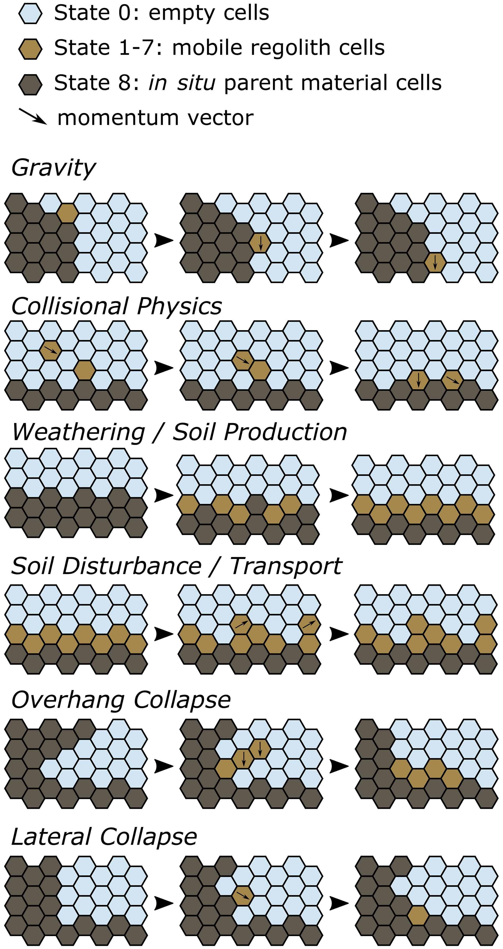
Figure 3Illustration of a “cellular automata” type of model used to simulate colluvial wedge formation. The figure shows geomorphic processes included in the model for air, mobile regolith, and in situ parent material cells (following Tucker et al., 2016, 2018, 2020). Definitions for “mobile regolith” and “in situ parent material” are given in Sect. 2.1.
Within Grain Hill, we generate a grid with hexagonal cells. Each cell within the model grid can consist of one of nine states. State 0 is empty air, states 1–6 represent “mobile regolith”, with momentum in one of six directions, state 7 represents mobile regolith at rest, and state 8 is “in situ material” or cells that represent uneroded parent material. Each mobile regolith cell is assumed to represent small aggregates of sedimentary material or individual clasts that can be mobilized by gravity, such as dry raveling, and/or mobile-regolith-disturbing processes, such as bioturbation. The in situ material cells are abstractions used to represent parent material that is stationary unless a mobile regolith production process or a collapse process converts it into mobile material. The in situ material cells are not distinguished by lithology, such as between crystalline bedrock or consolidated sedimentary material (e.g., alluvium), instead assuming that differences between lithologies can be represented by differences in geomorphic process rates.
For our goal of a generalized model, we chose to focus on geomorphic processes that appear to be consistent across the majority of colluvial wedges, i.e., colluvial processes, while avoiding site-specific processes such as fluvial deposition. We find that the minimum processes needed to produce colluvial wedges are mobile regolith production (rate given as W0 with units of yr−1), sometimes referred to as soil production in the geomorphology literature (e.g., Heimsath et al., 1997), mobile regolith disturbance (rate given as D with units of yr−1), roughly equivalent to “soil diffusivity” (as frequently described in process geomorphology; Culling, 1963; Furbish et al., 2009; Tucker et al., 2016), and gravitational collapse (rate set by gravity g converted to cellular automata transitions with units of yr−1 per Tucker et al., 2018). The former two processes are well-established geomorphic transport laws in process geomorphology (Dietrich et al., 2003; Tucker et al., 2016). The latter process, gravitational collapse, is treated in a straightforward manner as described below. With this philosophy, we use the cell states, cell interactions (mobile regolith production and disturbance), and gravitational collapse from Grain Hill. Furthermore, we extend the Grain Hill gravitational collapse process to include lateral collapse, whereby an in situ parent material cell can transition into a moving mobile regolith cell if it is laterally next to an air cell (lateral collapse rate – LCR – set as a fraction of gravity g converted to cellular automata transitions). Further discussion of non-included processes, such as pedogenesis, is in the Discussion.
The model's initial conditions start (Fig. 4) with a plane of in situ material (cell state 8) with a 5.71∘ initial slope (10 % gradient) overlain by air cells (state 0). The cell size is set to 2.5 cm to attempt a balance between the resolution of the model run, computational time, grain size of coarse alluvial fan material common to normal fault zones, and the approximate size of ped-like aggregates of mobile regolith. This cell size allows for adequate resolution to model disturbance process acting throughout the thickness of the mobile regolith. Alternate cell sizes (0.025–10 cm; Supplement) yield changes in the spatial resolution of the results but similar patterns of overall colluvial wedge morphology, transport, and velocity. We create a small one-cell-thick layer of mobile regolith on the pre-rupture ground surface to simulate a pre-existing surface soil layer. While a thicker mobile regolith layer may be more realistic for some field sites, a soil or mobile regolith layer's pre-earthquake thickness is tied to the timescale of surface stability and thus earthquake recurrence interval. As noted above, the effects of recurrence interval on colluvial wedge evolution deserve focused study and are thus not explored here. Next, we introduce a single faulting event that produces a 2 m high fault scarp (Fig. 4), consistent with historical earthquake surface ruptures (e.g., Crone et al., 1987a, b; Caskey et al., 1996). This approximate scarp size is consistent with M∼7 normal-faulting earthquakes (Wells and Coppersmith, 1994) as well as estimates of per-event displacement observed along multi-segment normal faults such as the Wasatch fault (2.0 m average displacement observed at 20 paleoseismic sites; DuRoss et al., 2016; Bennett et al., 2018). Although normal-faulting events can be larger, this scarp height allows us to capture detail in the resulting depositional features while keeping computational demands reasonable.
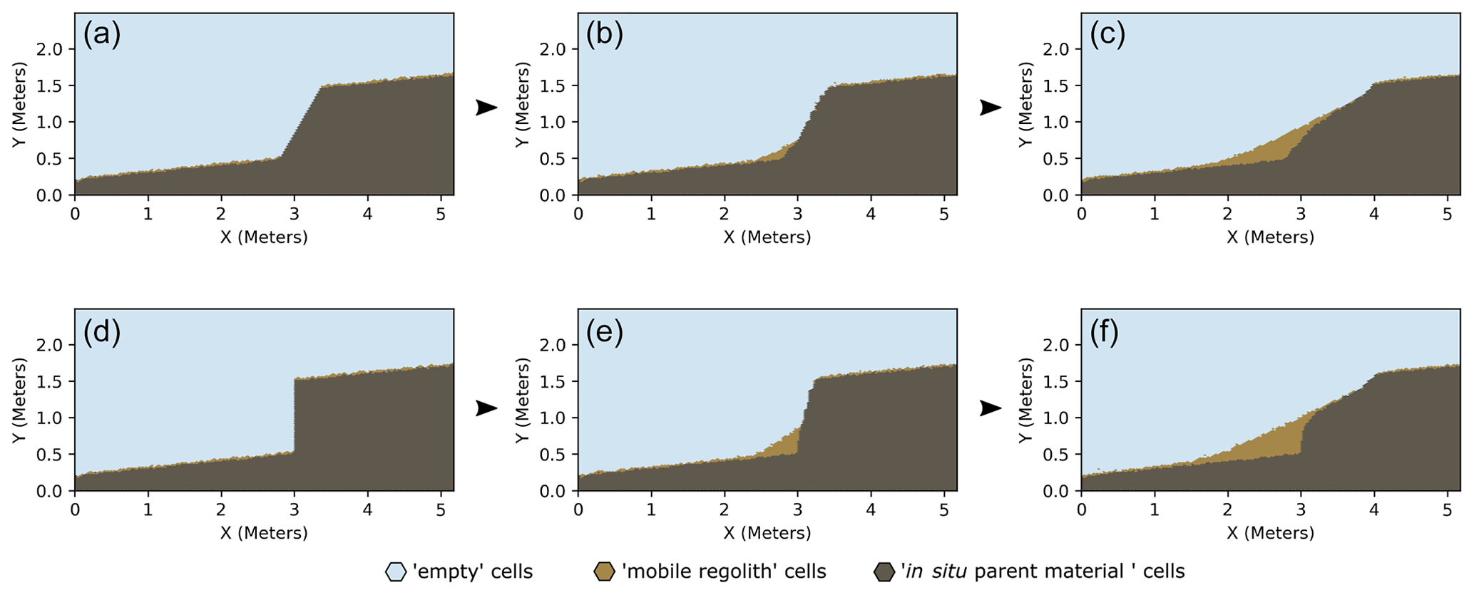
Figure 4Example of the evolution of the colluvial wedge cellular automata models for a 60∘ dipping fault (a, b, c) and for a vertical fault (d, e, f). In both models, there is an initial collapse whereby the fault face produces a layer of rapidly deposited mobile regolith cells that create a small wedge with a slope approximate to the angle of repose (30∘). The collapse phase is followed by a period of gradual deposition of mobile regolith cells that create an overall elongate wedge.
Following the initialization, we model 2000 years to capture the timescales of wedge formation (Wallace, 1977; McCalpin, 2009). Here, we model a single colluvial wedge to explore spatiotemporal trends in wedge formation and to avoid unnecessary complications related to repeated ruptures through older colluvial deposits. Note that the concept of a steady-state form is not applicable here as colluvial wedges are fundamentally transient features. Thus, a fixed model run time is needed and the resulting deposits must be analyzed with this in mind. We simulate both a vertical (90∘) fault and a 60∘ dipping fault to capture two end-member colluvial wedge morphologies. The 60∘ end-member is consistent with Anderson's theory of faulting from tectonics (Anderson, 1877) and seismic observations (e.g., Jackson and White, 1989), whereas the 90∘ fault is based on the near-surface refraction of normal faults to steeper dips as commonly observed in paleoseismic exposures (e.g., Machette et al., 1992).
For the unconstrained parameters in mobile regolith production, mobile regolith disturbance, and gravitational collapse, we vary the rate of input parameters over 4 orders of magnitude and observe the resulting colluvial wedge form. We picked these magnitudes from the observed range in mobile regolith diffusivity across the globe (i.e., Richardson et al., 2019) and convert this range into mobile regolith disturbance rate following equations in Tucker et al. (2018). To obtain a range for mobile regolith production rate, we note that the soil Péclet number, a measure of the relative magnitude of mobile regolith disturbance versus production, appears to fall into a range of 0.1–1 in global compilations, meaning that the orders of magnitude are roughly comparable (Gray et al., 2020). As such, we test the parameter space over a similar range as the mobile regolith disturbance rate. For the gravitational collapse, we let the mobile regolith cells overhanging air cells to collapse at a rate of free fall following Tucker et al. (2016). For our lateral collapse process, we explored 14 orders of magnitude over which the rate had a visible effect on the modeled colluvial wedge form. From this large parameter space, we picked 4 orders of magnitude (10−3, 10−5, 10−9, and 10−11 g, where g is the rate of gravity in cellular transitions per time following Tucker, 2016).
2.2 Facies definitions and transport metrics based on cell tracking
Comparing the numerical model with real-world observations of colluvial wedge sediment is challenging as the mobile regolith cells do not record information such as sedimentary texture (i.e., grain size, grain shape, sorting, or clast orientation) that is typically used to distinguish between various sedimentary facies. An alternative is to classify the types and durations of movements that occur in mobile regolith cells in the model and relate these as analogies to real-world facies. For example, clasts within the debris facies of a colluvial wedge (Nelson, 1992) likely experience greater transport in the vertical direction than in a horizontal direction, and transport likely occurs over a relatively short time. Conversely, sediment within the wash facies may be associated with greater overall horizonal transport than sediment in the debris facies and may occur over prolonged time periods.
To explore spatial patterns of cell movement, we conceive of a transport index (TI) to identify the movements and relative provenance of mobile regolith cells:
where Δy is the total vertical distance a mobile regolith cell has traveled and Δx represents the total horizontal distance, both following the scarp-forming earthquake. We chose this value as an index to evaluate mobile regolith cell motions because it informs the viewer of the mobile regolith cell's overall path. Note that the cellular automata model used here has an inherent angle of repose of 30∘ due to the hexagon shape of the cells (Tucker et al., 2016). Note that cells moving purely on an angle-of-repose slope have a transport index of (due to trigonometric right triangle relationships). As such, cells with a transport index greater than rad have likely spent more time in gravitational free fall than cells with values equal to or less than rad. The are being more likely to have traveled down an angle-of-repose slope.
Travel distance alone does not provide a complete picture of a mobile regolith cell's transport history. To further evaluate the transport histories of mobile regolith cells, we measure the total time spent in transport and the average transport velocity and give an example in Fig. 7. The total transport time measures the total time a mobile regolith cell has been in a moving state, which includes both gravitational free fall and the episodic motions due to mobile regolith disturbance and the resulting mobile regolith creep. The average transport velocity is the linear distance (calculated as ) divided by the total transport time (Fig. 8).
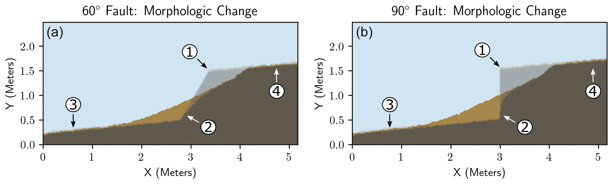
Figure 5Example of the change in fault-scarp morphology and colluvial wedge development in both the (a) 60∘ dipping fault and (b) 90∘ dipping fault. The transparent zone shows the initial fault scarp. See Figs. 3 and 4 for the legend. (1) The upper free face of the scarp erodes headward by both lateral collapse and by erosion from mobile regolith production as well as mobile regolith disturbance processes. A small knickpoint-like ledge may be visible if the scarp has not fully diffused. (2) A small trace of the fault free face is buried by the colluvial wedge, whereas the fault trace higher above has been eroded. The colluvial wedge volume is larger for the 90∘ dipping fault due to the increased accommodation space. (3) The mobile regolith on the hanging wall is partly buried by the colluvial wedge, whereas the still-exposed areas continue to develop over time. (4) The mobile-regolith-forming processes on the upthrown footwall continue and produce sediment that migrates downhill and is deposited onto the colluvial wedge.
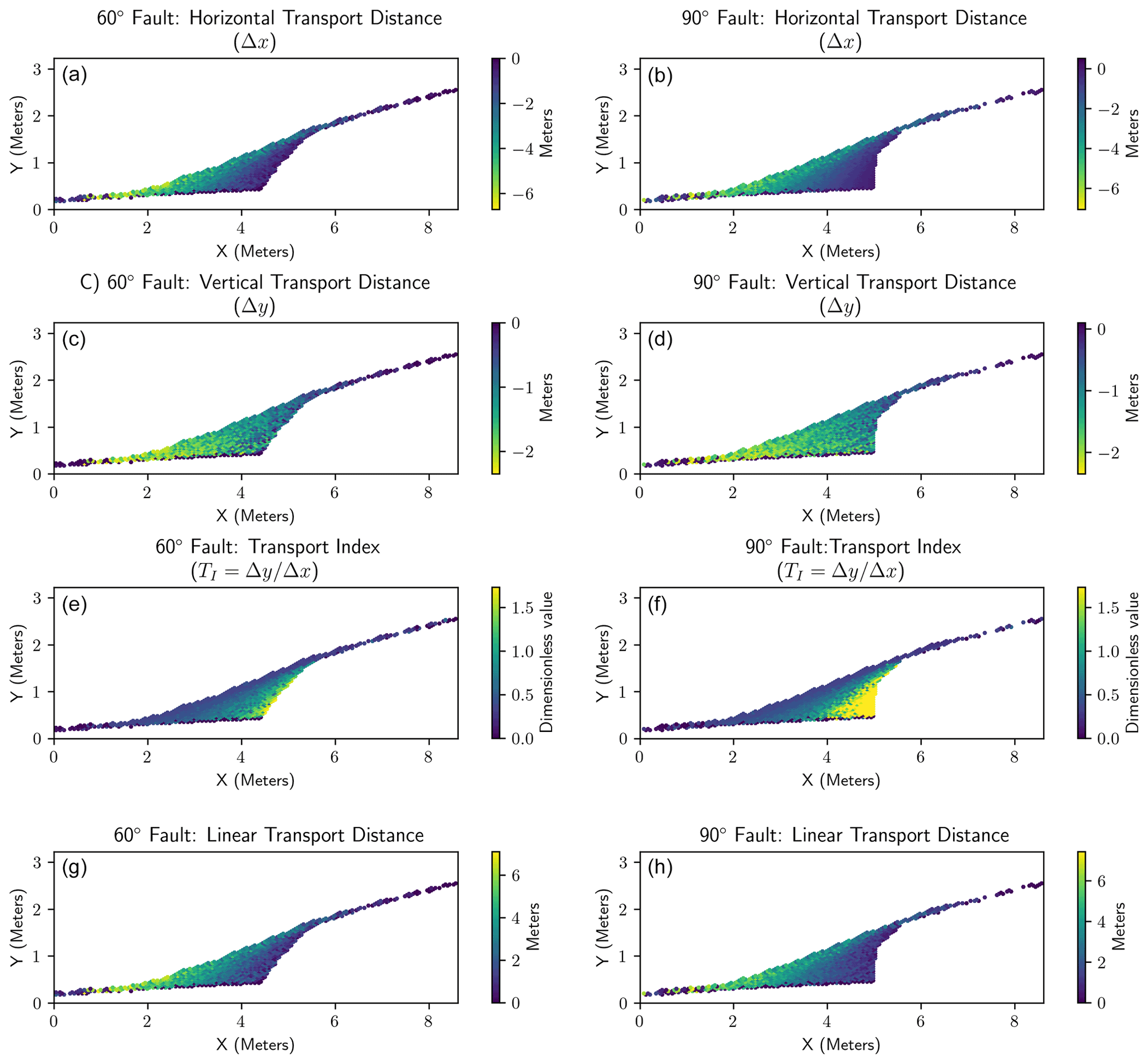
Figure 6Representative illustration of the horizontal and vertical displacements of the mobile regolith cells from the sensitivity analysis. See the Supplement for plots from the full parameter space. (a, b) Total horizontal displacement defined as the change in x position of a cell from the earthquake event until the end of the model run for the 60∘ fault (a) and the vertical fault (b). (c, d) Equivalent plots for the total change in the vertical y position. (e, f) Plots of the ratio (the transport index) between the total vertical movement and total horizontal movement. (g, h) Plots of the linear distance from the mobile regolith cell's original position at the start of the model run (linear distance: ).
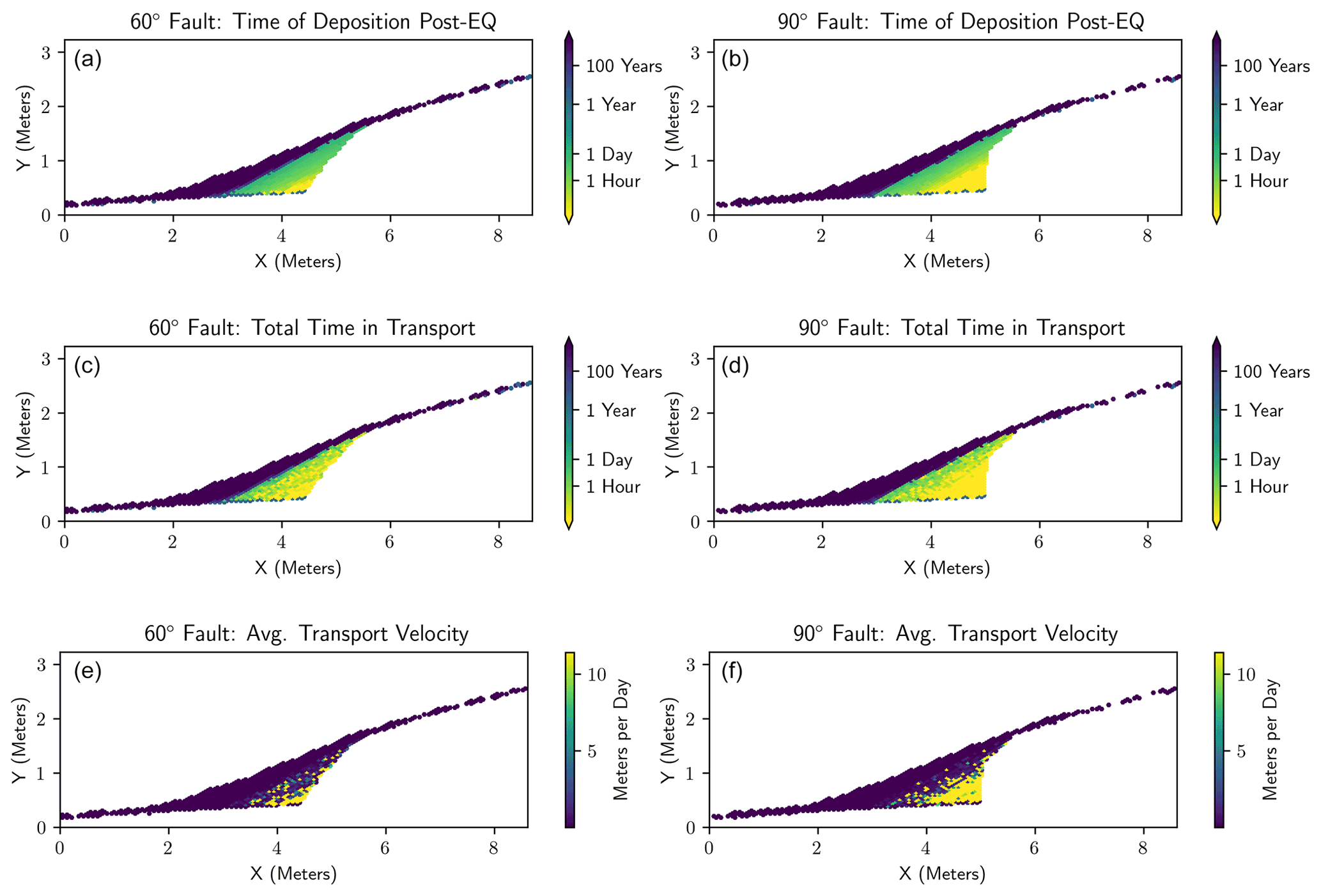
Figure 7Illustration of the timescales and rates of mobile regolith cell transport. See the Supplement for plots from the full parameter space. (a, b) Plots of the time of deposition following the scarp-forming earthquake. (c, d) The total time a mobile regolith cell spends in transport before coming to rest and burial. For both the 60∘ (a) and 90∘ faults (b), the colluvial wedge appears to have mostly developed within 1–10 model years. Some model runs with high relative collapse rates can produce a rapid initial deposit within hours to days. This rapid initial deposit is buried relatively slowly over hundreds of years until the modeled colluvial wedge reaches its maximum volume. (e, f) The average velocity of transport, calculated as the linear distance (a, b) divided by the total transport time (c, d). The higher average velocity indicates that the cell has traveled a significant distance in a relatively short period of time (e.g., gravitational free fall) compared to those that travel similar or shorter distances over a longer period of time (e.g., mobile regolith creep). Note the higher number of high-velocity cells in the 90∘ versus the 60∘ fault.
Next, we produce scatterplots of the various tracked metrics described above and plot them for each model run. In some cases, the mobile regolith cells appear to form groupings based on their transport histories. We interpret these self-organized groupings as analogs for various colluvial wedge sedimentary facies. Using the average transport velocity as a cutoff, we classify cells with an average transport velocity greater than 10 m d−1 as “lower debris”, cells with greater than 1 m yr−1 but less than 10 m d−1 as “upper debris”, and cells with less than 1 m yr−1 as analogs for lower debris facies, upper debris facies, and wash facies. The upper threshold for lower debris facies is the approximate average velocity of a hex cell state that travels almost entirely by gravitational free fall, with a smaller component of movement due to impacts and/or rebound from other free-falling cells, and thus more likely to be debris. The lower threshold of 1 m yr−1 is meant to exclude hex cell states largely traveling by raveling down the wedge slope. These values allow us to broadly encompass and classify the groupings observed in the scatterplots. Future work could focus on a mechanistic explanation for the observed groupings. Finally, we evaluate the effects of the geomorphic variables (mobile regolith production rate, mobile regolith disturbance rate, and lateral collapse rate) on the colluvial wedge morphology and distribution of sedimentary facies.
2.3 Sensitivity analysis and parameter space exploration
We test the sensitivity of select parameters on the colluvial wedge morphology using the transport index, total transport time, and average velocity as metrics. Since the number of parameters is large, the full parameter space requires excessive computational time, with many possible outcomes falling outside the realm of realistic geologic behavior. Instead we choose to focus on the dip of the fault, mobile regolith disturbance rate, mobile regolith production rate, and lateral collapse rate, as these appear to be key parameters controlling the colluvial wedge depositional environment. Parameters we keep constant are the height of the scarp (2 m), the size of the hex cells (2.5 cm), the time of a model run (2 kyr), and the initial slope of the faulted surface (5.7∘ 10 % slope). We also fix the Grain Hill friction factor to an assumed value of 0.25 per Tucker (2018) to include some elastic and/or momentum effects from inter-cobble collision, noting that this does not appear to have a major impact on the model results. An exploration of the fixed parameters would provide a useful perspective on the preservation potential of variously sized earthquake ruptures across different depositional environments. We leave these for future research as the goal here is to obtain a general understanding of how colluvial sediment transport variables influence colluvial wedge stratigraphy. The results of the parameter space exploration and sensitivity analysis are given in the Supplement.
3.1 Modeled colluvial wedge morphology
Running the model across the parameter space produces a triangular deposit of mobile regolith cells located at the base of the modeled scarp (Figs. 4, 5; see the Supplement for full parameter space). During the initial stages of the run, the fault face collapses and produces a small wedge of mobile regolith cells rapidly deposited within about a meter distance of the scarp. This rapid depositional phase is followed by a period of gradual deposition of mobile regolith cells, which eventually fill the available space between the top of the now-eroded scarp and the lower surface (Figs. 4, 5). The overall wedge for the 60∘ dipping fault is lower in total number of cells than the 90∘ fault scarp. The overall lengths of the modeled colluvial wedges are similar and both scarps show similar levels of headward erosion in later time steps of the models.
The overall displacement of individual cells is shown in Fig. 6. Both 60 and 90∘ fault models show a greater amount of total horizontal movement for mobile regolith cells in the distal parts of the wedge versus the fault-proximal zone. The total vertical movement is similar, with the distal parts of the wedge having mobile regolith cells with longer travel distances. The transport index, being a ratio of the vertical movement to the horizontal movement of a mobile regolith cell, shows a notable contrast between the 60∘ and vertical faults, with the vertical fault model showing a much larger zone of high (>1.5) transport index values. In contrast, the 60∘ fault model has a small zone of high transport index values mostly immediately adjacent to the fault. In both models, the zone of high transport index values is overlain by layers of mobile regolith cells with progressively lower transport index values that grade toward the surface of the wedge. After the colluvial wedge has filled the available accommodation space between the lower surface and the top of the fault scarp, there is an uppermost surficial layer of mobile regolith cells with consistent transport index values. The overall linear distance of transport (Fig. 7a, b) is consistent with the above observations.
A representative example of the temporal aspects of the path of individual cells is given in Fig. 7. In both 60∘ and 90∘ fault models, there is a large wedge shape of mobile regolith cells with short (<1 year) transport times overlain by a layer of cells with longer transport times (> 1–100 years). The relative pattern of the transport times appears fairly consistent throughout the parameter space, although the details vary based on the geomorphic process rates. The patterns of the average transport velocities generally consist of a wedge-shaped thin deposit of higher-velocity cells overlain by a thicker layer of lower-velocity cells. Sometimes, a layer of low-velocity cells is present within the overall high-velocity zone. The pattern of the average transport velocities across the parameter space can vary as the size of the higher-velocity zone appears to increase with an increase in lateral collapse rate and mobile regolith production rate. Finally, we plot interpreted sedimentary facies on the model results using the classification criteria in the Methods section (Figs. 8, 9, 10). Generally, the 60∘ dipping fault creates a relatively small zone of debris facies overlain by wash facies of varying thickness. In contrast, the 90∘ fault is much more likely to create a relatively larger zone of debris facies.

Figure 8Scatterplots of the various transport histories of mobile regolith cells (total transport time, transport index (, and average transport velocity). (a–d) Transport time versus transport index for various lateral collapse rates (LCRs). (e–h) Transport time versus linear distance for various lateral collapse rates. (i–l) Average transport velocity versus transport index. The scatterplots appear to show natural groupings of cells with similar transport histories. The color indicates our interpreted groupings of cells into analogs for the various sedimentary facies in the colluvial wedge model. These groupings are arbitrarily divided by the transport velocity with values greater than 105 m d−1 being “lower debris” analog facies and cells with values lower than 1 m d−1 being “wash” facies analogs. Cells between these values are classified as “upper-debris-facies” analogs.
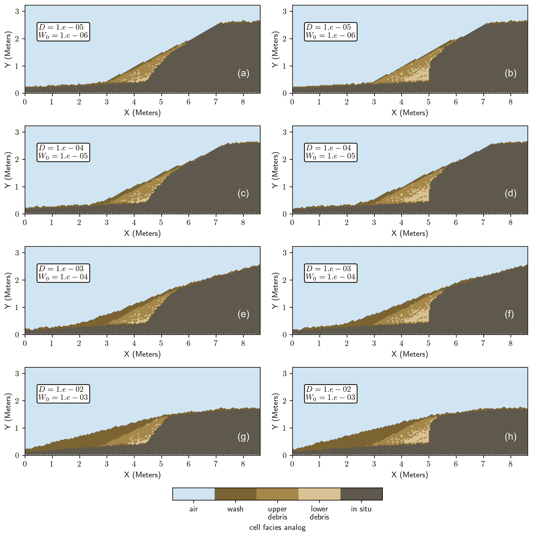
Figure 9Example illustration of modeled colluvial wedges and facies analogs for 60 and 90∘ faults per varied geomorphic process rates with a fixed lateral collapse rate of 10−5 g (see Fig. 3: D: disturbance rate, W0: mobile regolith production rate). Order of magnitude changes in the geomorphic process rates result in different wedge forms and stratigraphy.
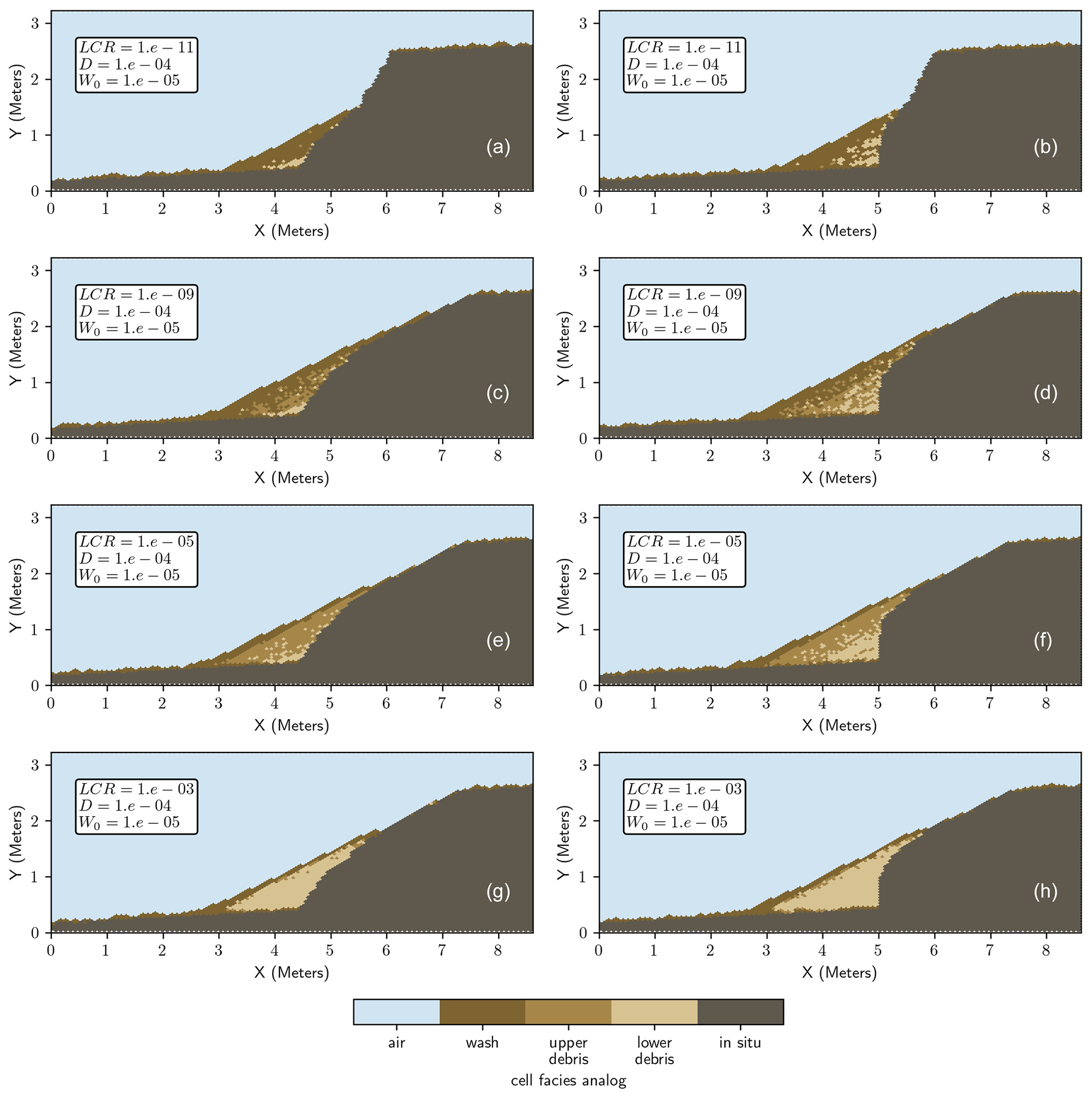
Figure 10Example illustration of a modeled colluvial wedge with sediment facies analogs for 60∘ and vertical fault planes as a function of lateral collapse rate (LCR). The lateral collapse rate is taken as a fraction of gravity, e.g., LCR 1e-05 is a rate of 10−5 times gravity entered into the lateral collapse function (Fig. 3). Higher collapse rates generally promote larger colluvial wedges and larger volumes of debris facies versus wash facies for a given geomorphic process rates (D, W0).
3.2 Colluvial wedge sensitivity to mobile regolith disturbance rate, mobile regolith production rate, and lateral collapse rate
Each of the three modeled geomorphic processes – mobile regolith disturbance, mobile regolith production, and lateral collapse – affect the morphology and stratigraphy of the resulting modeled colluvial wedge. First, the total area (number of mobile regolith cells) of the wedge represented by the model appears to be sensitive to all three parameters (Figs. 11, 12). Both mobile regolith production rate and lateral collapse rate broadly share a positive relationship with colluvial wedge area for any collapse rate. Higher collapse rates broadly create larger wedges, but this effect appears to be limited by the number of collapsible in situ parent material cells. The 90∘ fault appears to always create a larger colluvial wedge relative to the 60∘ fault, likely due to greater accommodation space.
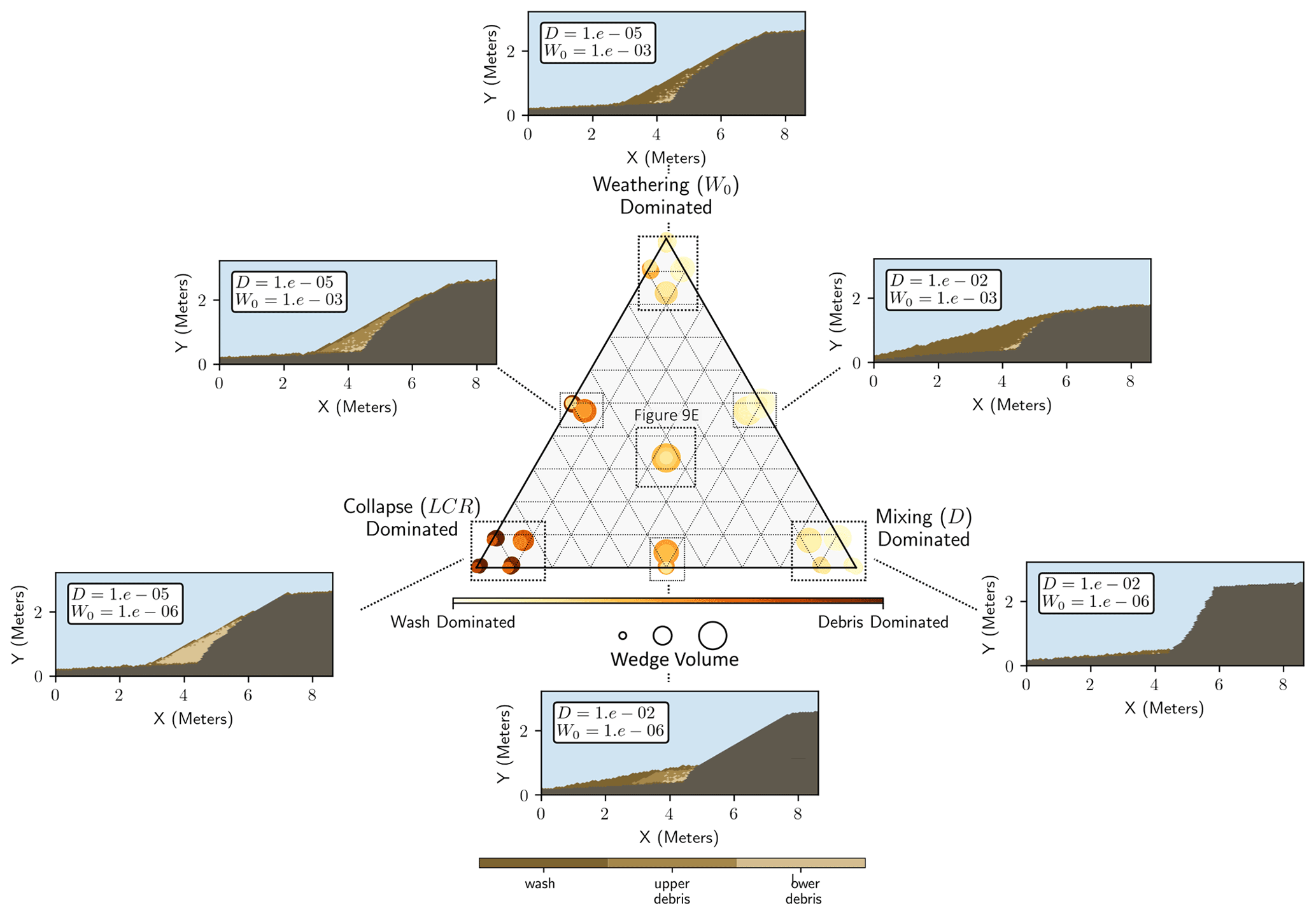
Figure 11Summary ternary diagram of the effects of geomorphic processes on colluvial wedge morphostratigraphy for the 60∘ fault model. Ternary axes are plotted as , where X is the axis variable (LCR, W0D). The color and size of points are scaled by relative quantity of facies and colluvial wedge size. The inset model runs show representative examples of wedges resulting from plotted parameter values.
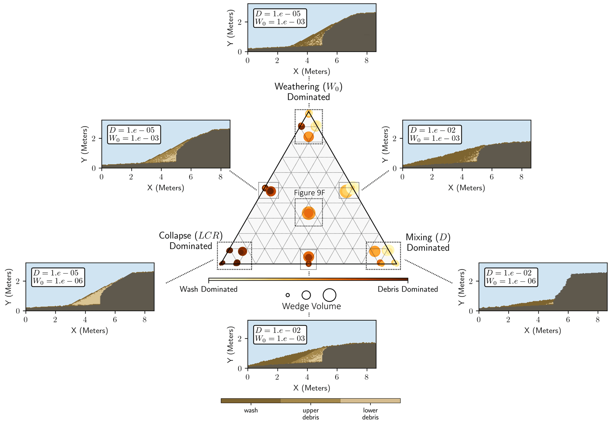
Figure 12Summary ternary diagram of the effects of geomorphic processes on colluvial wedge morphostratigraphy for the 90∘ fault model following Fig. 11. Note the greater quantity of debris facies relative to the 60∘ fault scenarios (Fig. 11).
The mobile regolith disturbance rate (D; Figs. 11, 12), the process whereby mobile regolith cells can be randomly moved by bioturbation (Fig. 3), for example, has a more nuanced affect: in model runs wherein the sediment supply is high due to raised mobile regolith production (W0) or lateral collapse (LCR), an increase in mobile regolith disturbance will increase the total size of the colluvial wedge and expose in situ parent material to further mobilization. In sediment-limited conditions such as lower mobile regolith production rate (W0), higher mobile regolith disturbance rates can decrease colluvial wedge volume by mobilizing sediment away from the fault scarp. This effect but can be seen in Figs. 11 and 12 for disturbance-dominated wedges. Relatively high mobile regolith disturbance rates can eventually remove the entire wedge deposit if there is no mobile regolith production to replenish it, and in some cases, the high mobile regolith disturbance rate works in tandem with high mobile regolith production to erode much of the fault scarp instead of lateral collapse (see extended results in the Supplement).
The ratio of the total area of the upper debris and lower debris facies (herein total debris facies) to the quantity of the wash facies is sensitive to geomorphic variables (Figs. 11 and 12). First, the 90∘ fault often creates a higher ratio of debris to wash facies than in the 60∘ fault, likely due to the greater number of collapsible cells in the 90∘ fault case. Likewise, higher lateral collapse rates appear to increase the amount of debris relative to wash facies. Next, an increase in the mobile regolith disturbance rate and/or the production rate appear to increase the quantity of wash facies relative to the total debris facies. This occurs due to the mobile regolith disturbance process reworking the post-collapse debris-like mobile regolith cells. In model runs with high mobile regolith disturbance relative to lateral collapse rates (Figs. 11, 12), the total debris facies can be almost entirely reworked, thus producing cell transport histories meeting our wash facies criteria. Finally, although subtle, the mobile regolith production rate decreases the relative amount of debris by producing large relative amounts of mobile regolith that then travel down the scarp into the colluvial wedge.
Our primary goal in this study is to evaluate model results to infer the theoretical effects of geomorphic process rates on colluvial wedge stratigraphy. However, the model here does have limited – but useful – explanatory power (sensu Bokulich, 2011) in that it provides a connection between field-based knowledge of conceptual colluvial wedge formation and the physics-based principles of sediment transport from process geomorphology. First, we must evaluate the realism of the model with respect to observations of colluvial wedge formation, both modern and observed in paleoseismic trenching of fault zones. Next, we must confirm if our choice of classification of mobile regolith cells into sedimentological facies designations is accurate and if they produce patterns that match our conceptual model of colluvial wedge formation. After this, we will describe the implications for colluvial wedge formation and interpretations. Note that here, sediment refers to real-world colluvial wedge material and mobile regolith refers to the modeled cells. While technically we are discussing the transport histories of mobile regolith cell states, we will refer to them as mobile regolith cells for colloquiality even though the cells themselves are stationary.
4.1 Model realism
The most basic validation one can make is that the model resembles colluvial wedges observed along historic and prehistoric fault scarps, those revealed in paleoseismic exposures, and the idealized form in the colluvial wedge conceptual model. The profile of the developed scarp is similar in appearance to modern examples of colluvial wedge formation, such as observed following the 1983 Borah Peak rupture (Crone et al., 1987; McCalpin et al., 1993; Arrowsmith and Rhodes, 1994; e.g., Fig. 2 versus Fig. 4, Figs. S1–S8). The full parameter space we explore produces fault scarps that range from essentially no wedge development up to almost complete erosion of the fault scarp, although we focus on runs most resembling real colluvial wedges (Figs. 9 and 10). The modeled wedges here bridge much of the gap between the classic wedge-shaped forms of the colluvial wedges (Wallace, 1977; Nelson, 1992; McCalpin, 2009, their Fig. 4.11) and forms that resemble a continuous mobile regolith layer with active transport (e.g., Bennett et al., 2018; DuRoss et al., 2018; Gray et al., 2019). We argue that the agreement between the model and previous theory and observations is evidence that the model is providing a reasonable analog of colluvial wedge development. Although the resemblance to real or idealized colluvial wedges does not prove that the underlying model mechanics are correct, the use of established geomorphic transport laws to reproduce the idealized forms described in the colluvial wedge conceptual model (Nelson, 1992; McCalpin, 2009) provides a mechanistic explanation for colluvial wedge formation and morphology.
Next, we must assess if the transport of mobile regolith cells conforms to field observations and previous theory. First, as noted in the results, the transport histories of mobile regolith cells form groupings that are not explicitly coded into the model (Fig. 8). These groupings arise because of the sediment transport physics from established geomorphic transport laws and/or the interactions of the cells as the model run progresses (Fig. 8). Because these groupings appear distinct, we classify them into analogs for the apparently similar sedimentary facies defined in the colluvial wedge literature by Nelson (1992). Note that Nelson's (1992) facies are based largely on arid-region colluvial wedges, and variance in facies across climate zones appears likely. An analysis of our sedimentary facies interpretations is provided in Sect. 4.3 below. The grouping of mobile regolith cells we classify into lower debris facies (Fig. 8) appear to be derived from relatively proximal sources (higher TI values, lower linear distance values), such as material from the fault scarp, and have overall short transport times. We suggest this would match the poorly sorted sediment of real-world lower debris facies.
The grouping of cells we classify into the upper debris facies show similarly proximal provenance but longer overall transport times (Fig. 8). This upper debris facies involves material from collapse and headward erosion of the scarp as well as reworking of the previously deposited lower debris facies. It should be noted that both upper debris and lower debris facies do not always occur subsequently and that interbedded layers of either, sometimes even including wash-like layers, can occur as a function of the relative geomorphic process rates (Figs. 9, 10). The similarity between the facies in the model and sedimentary facies provides a mechanistic explanation for the complex stratigraphy observed in actual colluvial wedges (Figs. 2, 9, 10).
Finally, the grouping we classify into wash facies is represented by distal provenance, long transport times, and low average velocity of transport (Fig. 8). Presumably, the effects of the transport histories represented by the wash facies analog cells would result in the better-sorted and finer-grained sediment observed in real colluvial wedges wash facies. The match-up between our modeled facies and real-world facies suggests agreement between the model and interpretations of colluvial wedge development through sedimentary analysis (Nelson, 1992; McCalpin et al., 1993; McCalpin, 2009).
The timescales of modeled versus actual colluvial wedge development must also be considered when assessing model realism. First, many of the model runs with higher collapse rates produce lower and upper debris facies cells rapidly, with some developing in approximately ≤ 10 years (Fig. 10g, h). At the highest collapse rates, the fault scarp fails immediately after the formation of the fault scarp, consistent with observations of modern wedges (Fig. 1; Wallace, 1977; McCalpin, 1993). This initial collapse phase is followed by a longer period of deposition (up until the end of the model run of 2000 years) and is associated with longer-term processes such as reworking of debris facies and production of the rest of the wash facies (Fig. 7c, d). These timescales appear to broadly match expectations of wedge development (Forman et al., 1988, 1991; McCalpin, 2009). When collapse rates are lower, or at least of comparable magnitude to mobile regolith disturbance rates, more complex stratigraphy can be produced with layers of cells matching upper or lower debris facies criteria. Some model runs appear to show layering from individual collapse events interspersed with reworked mobile regolith cells (Fig. 10b, d). Such a system appears to create stratigraphy that may resemble multiple small earthquakes rather than one large event. This result may imply that the stochastic nature of collapse means that, theoretically, a single earthquake event could produce apparently multi-earthquake stratigraphy if geomorphic process rates allow, at least within the domain of our model conditions.
From these observations, we argue that this model can reasonably reproduce colluvial wedge morphologies and gross sedimentary facies over realistic time frames. Furthermore, the model we describe here offers a way to connect colluvial wedge theory to the first-principles physics of sediment transport. We conclude that the model can be used to hypothesize how changes in geomorphic variables affect colluvial wedge development with some limited mechanistic explanatory power for the idealized colluvial wedge conceptual model.
4.2 Sensitivity to geomorphic parameters
Our results suggest that, theoretically, geomorphic variables (i.e., mobile regolith production rate, mobile regolith disturbance rate, and lateral – free-face – collapse rate) directly impact colluvial wedge form and sedimentology. The most significant theoretical result from this study is that facies distributions may not necessarily occur in a sequential order. Interbedding of layers with different transport histories is possible, particularly when collapse rates are low (Figs. 9, 10). Other researchers (e.g., Gray et al., 2019) have noted site-specific field relations that suggest greater complexity behavior in real colluvial wedges than is currently represented in the colluvial wedge conceptual model. A possible consequence of complex behavior is that a single faulting event could theoretically produce multiple facies sequences that resemble discrete faulting events, despite only a single event occurring. Whether this happens in real-world situations remains to be tested, but the possibility may complicate paleoseismic hazard assessments. However, this may be avoided by soil profile and geochronological interpretations (e.g., Berry, 1990).
Other theoretical effects of geomorphic parameters match interpretations present in the literature. For example, the debris facies in the model can form either due to the lack of internal cohesion of the parent material (high rates of lateral collapse) or due to mobile-regolith-forming processes acting on the exposed free face, similar to interpretations by Wallace (1977). Such mobile-regolith-forming or regolith-disturbing processes could involve burrowing mammals, root growth, shrink–swell, and freeze–thaw cycles among many others (Gray et al., 2020). Another example is the field-observed effect of microclimate on scarp degradation whereby aspect-controlled water contents affect the degradation rate (e.g., Pierce and Colman, 1986; Pelletier et al., 2006). In the model, such variance in degradation rate can be reproduced by varying the relative geomorphic parameters, noting that the specific recreation of a field site is beyond the scope of the model.
Additionally, depending on the rates of geomorphic processes, the colluvial wedge could theoretically undergo substantial reworking that in turn affects information on earthquake timing such as that recorded by geochronology. For example, model runs with high relative mobile regolith disturbance rates appear to substantially rework the initially deposited debris facies, converting some fraction of it into wash facies over time. When mobile regolith disturbance rates sufficiently exceed mobile regolith production and lateral collapse rates, the entire wedge can be converted into the wash facies classification given enough time. One could reasonably surmise that geochronometers such as 14C and OSL (optically stimulated luminescence) would produce younger ages via incorporation of more recent carbon and sunlight exposure. The extent to which this happens in nature is debatable. Generally, mobile regolith disturbance processes are linked with mobile regolith production processes (Wilkinson et al., 2009; Roering et al., 2010) such that the relative magnitude of both disturbance and production appears to be relatively constant across climate zones (Gray et al., 2020). However, one could imagine a fault scarp in highly cohesive material (low collapse rates) in an arid climate with low mobile regolith production rates, but with high disturbance rates with burrowing desert fauna. Such a case may be testable with a meta-analysis of geochronology from paleoseismic studies.
As the rates of mobile regolith production and mobile regolith disturbance play a large role in colluvial wedge form, we should acknowledge when such values are expected to be high versus low. There is evidence that wetter climates with higher mean annual precipitation can have higher mobile regolith disturbance rates than drier climates assuming that mobile regolith disturbance is coincident with mobile regolith transport rates (see data in Richardson et al., 2019: their Fig. 2). Similarly, higher mobile regolith disturbance rates may be associated with locations of higher mobile regolith production rates because the processes that disturb mobile regolith are often the same or closely related to the processes that create mobile regolith (Gray et al., 2020). Based on the model results, the wash-dominated colluvial wedges created with higher mobile regolith disturbance and production rates may be associated with wetter climates including microclimates (Pierce and Colman, 1986; Pelletier et al., 2006). Conversely, our model runs that produce debris-dominated colluvial wedges are often associated with lower values of mobile regolith production or disturbance. A reasonable hypothesis following these observations is that climate may impact the sedimentology of a colluvial wedge for a given lithology. Consequently, an earthquake may produce a different colluvial wedge in a wetter climate versus a drier climate for the same given amount of displacement with all other variables held constant.
Finally, it is not just geomorphic variables that control colluvial wedge form. It is important to note that the tectonically controlled angle of the fault scarp appears to increase the sensitivity of the relationships between the geomorphic variables and the colluvial wedge morphostratigraphy (Figs. 10, 11). For example, the 90∘ fault contains a large propensity for collapse, whereas the gentler slopes of the 60∘ fault do not. Mobile regolith cells in the 60∘ fault tend to episodically tumble downslope via gravity, the overall rate of which depends on the presence of other mobile regolith cells on the fault scarp. If there is a significant number of mobile regolith cells on the slope, this can slow down the overall transport of a cell state. This impedes the rapid deposition of debris facies and causes the 60∘ fault to more likely consist of wash and lower-debris-facies cells (Figs. 9, 10), whereas the 90∘ fault hosts both wash, upper debris, and lower debris facies. As a final note, the steeper 90∘ fault generally creates taller and thicker colluvial wedges, likely due to the greater accommodation space created by the tall scarp, which suggests that estimates of fault displacement based on wedge thickness alone (e.g., Ostenaa, 1984; Klinger et al., 2003; McCalpin, 2009; Bennett et al., 2018; DuRoss et al., 2014, 2018) could be complicated by near-surface fault geometry.
4.3 Comparisons between the model facies and actual sedimentary facies
To make comparisons between the model and real colluvial wedge stratigraphy, we needed to first classify which mobile regolith cells are analogous to the various sedimentary facies in colluvial wedges. In this study, we chose classification criteria based on average transport velocity to divide mobile regolith cells into those resembling upper debris, lower debris, and wash facies. Although other subdivisions are possible with our model, such as those in the colluvial wedge conceptual model (e.g., Nelson, 1992), we did not pursue those to limit the influence of subjective criteria in our interpretations and to stay close to the general concepts of colluvial wedge development. The classification criteria we chose are based on the self-organized groupings of cell transport histories from the model runs (Fig. 8 and the Supplement). Admittedly, the sharp cutoffs in velocity value for each facies do not capture the apparently diffuse boundary between groupings seen in the scatterplots (Fig. 8). A potentially better method may be to use a statistical tool such as a mixing model, but it is beyond the scope of this study to explore this point further. However, we argue that the facies designations are reasonable boundaries for the self-organized groupings and allow us to use the model as a general analog for colluvial wedge morphostratigraphy
The modeled upper and lower debris facies largely resemble those described by the standard colluvial wedge facies model (Nelson, 1992). The modeled debris facies create a wedge-shaped zone that increases in thickness with proximity to the fault (Figs. 8, 9, S33–S40) similarly to natural debris facies. This initial deposit of colluvium helps preserve the original dip of the fault plane (exposed fault free face), which is steepest adjacent to the debris facies but becomes progressively more eroded and gently dipping where buried by wash facies sediment. As the cells in the model are uniform and there is not a clear way to model grain sorting, our separation between upper and lower debris facies in the model is largely based on transport characteristics. There are, however, similarities between the formation of the upper and lower debris facies in the model and hypothesized forming mechanisms reported by field-based studies (Wallace, 1977, Pierce and Colman, 1987, Nelson, 1992, McCalpin, 2009), namely that both lateral collapse of the free face and collapse due to mobile regolith production or disturbance (Fig. 12) can occur by the same processes. An example may be bioturbation i terms of both mixing soil and also inducing collapse via burrowing into the fault free face. Finally, there is agreement with the maximum timescales of the model's formation of the debris facies (<100 to <1000 years) and observations of modern to historical fault scarps (Wallace, 1977, McCalpin, 2009).
The modeled wash facies also have features that simulate their natural analog. First, the shape of the wash facies spans from very thin layers overlying the debris facies up to large elongate layers that reach their maximum thickness near the toe of the debris facies (Figs. 8, 9, S33–S40). In contrast to the modeled debris facies, the modeled wash facies tend to be constantly reworked and have lower average transport velocities and longer transport times. In many model runs, a persistent layer of active sediment transport exists near the surface of the wash facies similar to observed field relations (McCalpin, 2009; Gray et al., 2019). This persistent reworking by mobile regolith disturbance is analogous to the current model of wash facies development by bioturbation and sheet-wash processes (Nelson, 1992).
4.4 Implications and conclusions for colluvial wedge formation and interpretations
The methods and results presented here offer three implications for the state of knowledge on colluvial wedge development. The first is that the model can connect the observations of a wide variety of natural colluvial wedge morphology to a physics-based model that appears to accurately reproduce a large variety of colluvial wedge development. This means that despite the wide range in geomorphic mobile regolith production and disturbance processes at play in colluvial wedge environments, our general theory for their development (Wallace, 1977, Nelson, 1992, McCalpin, 2009) seems to be largely accurate. Although this is not a formal test of the colluvial wedge conceptual model (Wallace, 1977; Schwartz and Coppersmith, 1984; McCalpin, 2009), it provides support for the idea that observations of modern wedge development can be extrapolated into a theory of colluvial wedge development over geomorphic timescales using geomorphic transport laws (Nelson, 1992; Dietrich et al., 2003). A corollary of this implication is that the effects of just a handful of abstracted geomorphic processes (here, mobile regolith production rate, mobile regolith disturbance rate, and lateral collapse rate) can explain a wide variety of colluvial wedge forms. Although these parameters yield realistic wedges, testing how wedge morphostratigraphy responds to more complicated factors such as steep and/or variable surface topography, complex (e.g., distributed and antithetic) faulting, and repeated surface ruptures through time would further build confidence in relating physics-based models to natural colluvial wedge observations.
The second implication of this study is that the effects of fault plane angle, mobile regolith production, mobile regolith disturbance, and free-face collapse are important to consider when interpreting a sequence of colluvial wedge formation (Figs. 11, 12). The angle of the fault plane appears to play a large role, with the more steeply dipping fault planes leading to faster wedge development (Fig. 7), a larger proportion of debris facies (Figs. 8, 9, 12), and larger (thicker and more laterally extensive) wedge deposits (Figs. 8, 9, 10). As a result, in the case of repeated fault rupture, colluvial wedges along steeply dipping faults may be more likely to be identified and correctly interpreted as evidence of fault rupture than those along lower angle faults, which could be more difficult to differentiate given their reduced volumes. The higher rates of lateral collapse, say for unconsolidated parent material, correlate with the rapid development of debris facies (Fig. 12). However, high rates of mobile regolith production and disturbance on parent material with low collapse rates can also generate debris facies, although likely in a slower fashion.
Next, the model results provide a physics-based explanation and nuance for the findings of Wallace (1977), who documented fault scarps in field exposures across the American West. Wallace (1977) hypothesized that colluvial wedge formation occurs with a debris-dominated phase until the fault-scarp free face is buried, after which a more gradual period of lower-energy deposition continues until the eventual burying and topographic diffusive-like smoothing of the whole scarp. Our physics-based modeling confirms Wallace's colluvial wedge model, but only when lateral collapse rates are high relative to mobile regolith production and disturbance processes. When lateral collapse rates are comparable or relatively low, Wallace's (1977) hypothesized phases are less distinct, with collapse events occurring stochastically interspersed with periods of disturbance and reworking of wedge material. These interspersed periods of collapse and reworking largely appear to theoretically cause wedge facies stratigraphy to be less distinct than when collapse rates are high. The dependence of wedge facies stratigraphy on process rates provides an explanation for why some colluvial wedge exposures can show classic wedge-shaped forms (e.g., Jackson, 1991; DuRoss et al., 2018), whereas other exposures show less distinct but clearly colluvial wedge deposits (e.g., Bennett et al., 2018). Although not explored here, the topographic evolution of a fault scarp should also have this dependence on process rates, although the effect on fault-scarp diffusion dating methods is not yet clear.
Finally, the combined effects of the rates of mobile regolith production and disturbance can theoretically create interbedding in colluvial wedges. Multiple episodes of collapse and reworking can theoretically occur for a single earthquake event, although it seems that this would become less likely through time as the free face is progressively eroded and thus the source of collapse failure diminishes. Additionally, earthquake events with similar magnitude and displacement can have different colluvial wedges if the mobile regolith production and disturbance rates are different, say from a difference in climate or environment. This idea could be explored with models paired with meta-analysis of colluvial wedge shapes, sizes, and strata formed in different climates from the published literature. We hypothesize that geomorphic process rates control the extent of reworking, which may in turn affect the results of geochronology. Finally, as mentioned in the Introduction, the model presented here offers a potential new means to explore further questions on colluvial wedge development over timescales longer than the modern record.
The source code for the cellular automata Grain Hill model used in this study is publicly available in the open-source Zenodo repository (https://doi.org/10.5281/zenodo.1306961, Tucker, 2018).
The supplement related to this article is available online at: https://doi.org/10.5194/esurf-10-329-2022-supplement.
HJG designed, coded, and generated modeling results. HJG, CBD, SRN, and RDG analyzed results and wrote the paper.
The contact author has declared that neither they nor their co-authors have any competing interests.
Any use of trade, product, or firm names is for descriptive purposes only and does not imply endorsement by the US Government.
Publisher's note: Copernicus Publications remains neutral with regard to jurisdictional claims in published maps and institutional affiliations.
Thank you to Nadine Reitman, Katherine Barnhart, Philippe Steer, and Matan Ben-Asher for constructive comments that improved this paper.
This work was partially supported by the US Geological Survey Earthquake Hazards Program and the US Geological Survey National Cooperative Geologic Mapping Program.
This paper was edited by Greg Hancock and reviewed by Philippe Steer and Matan Ben-Asher.
Anderson, E.: The dynamics of faulting and dyke formation with applications to Britain, Oliver and Boyd, Edinburgh, 2nd edn., 1877.
Arrowsmith, J. and Rhodes, D.: Original forms and initial modifications of the Galway Lake Road scarp formed along the Emerson fault during the 28 June 1992 Landers, California, earthquake, B. Seismol. Soc. Am., 84, 511–527, 1994.
Arrowsmith, J., Rhodes, D., and Pollard, D.: Morphologic dating of scarps formed by repeated slip events along the San Andreas Fault, Carrizo Plain, California, J. Geophys. Res.-Sol. Ea., 103, 10141–10160, 1998.
Barnhart, K. R., Hutton, E. W. H., Tucker, G. E., Gasparini, N. M., Istanbulluoglu, E., Hobley, D. E. J., Lyons, N. J., Mouchene, M., Nudurupati, S. S., Adams, J. M., and Bandaragoda, C.: Short communication: Landlab v2.0: a software package for Earth surface dynamics, Earth Surf. Dynam., 8, 379–397, https://doi.org/10.5194/esurf-8-379-2020, 2020.
BenDror, E. and Goren, L.: Controls over sediment flux along soil-mantled hillslopes: Insights from granular dynamics simulations, J. Geophys. Res.-Sol. Ea., 123, 924–944, 2018.
Bennett, S., DuRoss, C., Gold, R., Briggs, R., Personius, S., Reitman, N., DeVore, J., Hiscock, A., Mahan, S., and Gray, H.: Paleoseismic results from the Alpine site, Wasatch fault zone: Timing and displacement data for six Holocene earthquakes at the Salt Lake City-Provo segment boundary, B. Seismol. Soc. Am, 108, 3202–3224, https://doi.org/10.1785/0120160358, 2018.
Berry, M.: Soil catena development on fault scarps of different ages, eastern escarpment of the Sierra Nevada, California, Geomorphology, 3, 333–350, 1990.
Bokulich, A.: How scientific models can explain, Synthese, 180, 33–45, 2011.
Bokulich, A.: Explanatory Models Versus Predictive Models: Reduced Complexity Modeling in Geomorphology, in: EPSA11 Perspectives and Foundational Problems in Philosophy of Science, edited by: Karakostas, V., Dieks, D., The European Philosophy of Science Association Proceedings, vol. 2, Springer, Cham, https://doi.org/10.1007/978-3-319-01306-0_10, 2013.
Caskey, S., Wesnousky, S., Zhang, P., and Slemmons, D.: Surface faulting of the 1954 Fairview Peak (Ms = 7:2) and Dixie Valley (Ms = 6:8) earthquakes, central Nevada, B. Seismol. Soc. Am., 86, 286–291, 1996.
Colman, S. and Watson, K.: Ages estimated from a diffusion equation model for scarp degradation, Science, 221, 263–265, 1983.
Crone, A., Machette, M., Bonilla, M., Lienkaemper, J., Pierce, K., Scott, W., and Bucknam, R.: Surface faulting accompanying the Borah Peak earthquake and segmentation of the Lost River fault, central Idaho, B. Seismol. Soc. Am., 77, 739–770, 1987a.
Crone, A., Machette, M., Bonilla, M., Lienkaemper, J., Pierce, K., Scott, W., and Bucknam, R.: Surface faulting accompanying the Borah Peak earthquake and segmentation of the Lost River fault, central Idaho, B. Seismol. Soc. Am., 77, 739–770, 1987b.
Culling, W. E.: Soil creep and the development of hillside slopes, J. Geol., 71, 127-161, 1963.
D'Ambrosio, D., Di Gregorio, S., Gabriele, S., and Gaudio, R.: A cellular automata model for mobile regolith erosion by water, Phys. Chem. Earth Pt. B., 26, 33–39, 2001.
Dietrich, W. E., Bellugi, D. G., Sklar, L. S., Stock, J. D., Heimsath, A. M., and Roering, J. J.: Geomorphic transport laws for predicting landscape form and dynamics, Geophysical Monograph-American Geophysical Union, 135, 103–132, 2003.
Doane, T., Roth, D., Roering, J., and Furbish, D.: Compression and decay of hillslope topographic variance in Fourier wavenumber domain, J. Geophys. Res.-Earth, 124, 60–79, 2019.
DuRoss, C., M.D. Hylland, G., Crone, A., Personius, S., Gold, R., and Mahan, S.: Holocene and latest Pleistocene paleoseismology of the Salt Lake City segment of the Wasatch fault zone, Utah, at the Penrose Drive trench site, in: Evaluating Surface Faulting Chronologies of Graben-Bounding Faults in Salt Lake Valley, Utah – New Paleoseismic Data from the Salt Lake City Segment of the Wasatch Fault Zone and the West Valley Fault Zone, Utah Geol. Surv. Spec. Stud, 24, 1–35, 2014.
DuRoss, C., Personius, S., Crone, A., Olig, S., Hylland, M., Lund, W., and Schwartz, D.: Fault segmentation: New concepts from the Wasatch fault zone, J. Geophys. Res, 121, 1131–1157, https://doi.org/10.1002/2015JB012519, 2016.
DuRoss, C., Bennett, S., Briggs, R., Personius, S., Gold, R., Reitman, N., and Mahan, S.: Combining Conflicting Bayesian Models to Develop Paleoseismic Records: An Example from the Wasatch Fault Zone, Utah, B. Seismol. Soc. Am., 108, 3180–3201, 2018.
Ferdowsi, B., Ortiz, C., and Jerolmack, D.: Glassy dynamics of landscape evolution, P. Natl. Acad. Sci. USA, 115, 4827–4832, 2018.
Forman, S., Nelson, A., and McCalpin, J.: Thermoluminescence dating of fault-scarp-derived colluvium: Deciphering the timing of paleoearthquakes on the Weber Segment of the Wasatch fault zone, north central Utah, J. Geophys. Res.-Sol. Ea., 96, 595–605, 1991.
Forman, S., Jackson, M., McCalpin, J., and Maat, P.: The potential of using thermoluminescence to year buried soils developed on colluvial and fluvial sediments from Utah and Colorado, USA, Preliminary results, Quaternary Sci. Rev., 7, 287–293, 1988.
Furbish, D. J. and Doane, T. H.: Rarefied particle motions on hillslopes – Part 4: Philosophy, Earth Surf. Dynam., 9, 629–664, https://doi.org/10.5194/esurf-9-629-2021, 2021.
Furbish, D. J., Schumer, R., and Keen-Zebert, A.: The rarefied (non-continuum) conditions of tracer particle transport in soils, with implications for assessing the intensity and depth dependence of mixing from geochronology, Earth Surf. Dynam., 6, 1169–1202, https://doi.org/10.5194/esurf-6-1169-2018, 2018.
Galli, P., Giaccio, B., Peronace, E., and Messina, P.: Holocene Paleoearthquakes and Early–Late Pleistocene Slip Rate on the Sulmona Fault Central Apeninnes, Italy, B. Seismol. Soc. Am., 105, 1–13, 2015.
Ghosh, P., Mukhopadhyay, A., Chanda, A., Mondal, P., Akhand, A., Mukherjee, S., and Hazra, S.: Application of Cellular automata and Markov-chain model in geospatial environmental modelling-A review, Remote Sensing Applications: Society and Environment, 5, 64–77, 2017.
Gray, B., Bloszies, C., Mcdonald, E., Page, W., and Baldwin, J.: Rethinking the colluvial wedge: a revised model for colluvial event stratigraphy in sloped environments, Geological Society of America Abstracts with Programs, 51, 4, https://doi.org/10.1130/abs/2019CD-329353, 2019.
Gray, H., Keen-Zebert, A., Furbish, D., Tucker, G., and Mahan, S.: Depth-dependent mobile regolith mixing persists across climate zones, P. Natl. Acad. Sci. USA, 117, 8750–8756, 2020.
Hanks, T., Bucknam, R., Lajoie, K., and Wallace, R.: Modification of wave-cut and faulting-controlled landforms, J. Geophys. Res.-Sol. Ea., 89, 5771–5790, 1984.
Heimsath, A. M., Dietrich, W. E., Nishiizumi, K., and Finkel, R. C.: The soil production function and landscape equilibrium, Nature, 388, 358-361, 1997.
Hobley, D. E. J., Adams, J. M., Nudurupati, S. S., Hutton, E. W. H., Gasparini, N. M., Istanbulluoglu, E., and Tucker, G. E.: Creative computing with Landlab: an open-source toolkit for building, coupling, and exploring two-dimensional numerical models of Earth-surface dynamics, Earth Surf. Dynam., 5, 21–46, https://doi.org/10.5194/esurf-5-21-2017, 2017.
Jackson, M.: The number and timing of Holocene paleoseismic events on the Nephi and Levan segments, Wasatch fault zone, Utah Spec. Stud. Utah Geol. Miner. Surv., 78, 1–23, 1991.
Jackson, J. and White, N.: Normal faulting in the upper continental crust: Observations from regions of active extension, J. Struct. Geol., 11, 15–36, https://doi.org/10.1016/0191-8141(89)90033-3, 1989.
Klinger, Y., Sieh, K., Altunel, E., Akoglu, A., Barka, A., Dawson, T., and Rockwell, T.: Paleoseismic evidence of characteristic slip on the western segment of the North Anatolian fault, Turkey, B. Seismol. Soc. Am., 93, 2317–2332, 2003.
Kogan, L. and Bendick, R.: A mass failure model for the initial degradation of fault scarps, with application to the 1959 scarps at Hebgen Lake, Montana, B. Seismol. Soc. Am., 101, 68–78, 2011.
Machette, M., Personius, S., and Nelson, A.: Paleoseismology of the Wasatch fault zone: A summary of recent investigations, interpretations, and conclusions, in: Assessment of Regional Earthquake Hazards and Risk Along the Wasatch Front, Utah, U.S. Geol. Surv. Prof. Paper 1500, edited by: Gori, P. and Hays, W., A1–A59, U.S. Gov. Print. Off, Washington, D. C., https://doi.org/10.3133/pp1500AJ, 1992.
Malde, H., Pitt, A., and Eaton, J.: Geologic investigation of faulting near the National Reactor Testing Station, Idaho, US Geological Survey Open-File Report, 167 pp., 2, https://doi.org/10.3133/ofr71338, 1971.
McCalpin, J. (Ed.): Paleoseismology, Academic press, 2nd edition View series: International Geophysics, ISBN 9780123735768, 2009.
McCalpin, J., Zuchiewicz, W., and Jones, L.: Sedimentology of fault-scarp-derived colluvium from the 1983 Borah Peak rupture, central Idaho, J. Sediment. Res., 63, 120–130, 1993.
Murray, A. and Paola, C.: A cellular model of braided rivers, Nature, 371, 54–57, 1994.
Nash, D.: Morphologic dating of degraded normal fault scarps, J. Geol., 88, 353–360, 1980.
Nash, D.: FAULT: A FORTRAN program for modelling the degradation of active normal fault scarps, Comput. Geosci., 7, 249–266, 1981.
Nash, D.: Morphologic dating of fluvial terrace scarps and fault scarps near West Yellowstone, Montana, Geol. Soc. Am. Bull., 95, 1413–1424, 1984.
Nash, D. and Beaujon, J.: Modelling degradation of terrace scarps in Grand Teton National Park, USA, Geomorphology, 75, 400–407, 2006.
Nelson, A.: Lithofacies analysis of colluvial sediments; an aid in interpreting the Recent history of Quaternary normal faults in the Basin and Range Province, Western United States, J. Sediment. Res., 62, 607–621, 1992.
Nelson, A., Personius, S., Sherrod, B., Kelsey, H., Johnson, S., Bradley, L., and Wells, R.: Diverse rupture modes for surface deforming upper plate earthquakes in the southern Puget Lowland of Washington State, Geosphere, 10, 769–796, 2014.
Ostenaa, D.: Relationships affecting estimates of surface fault displacements based on scarp-derived colluvial deposits, Geol, Soc. Am. Abstr. Progr, 16, 327, 1984.
Pelletier, J., DeLong, S., Al-Suwaidi, A., Cline, M., Lewis, Y., Psillas, J., and Yanites, B.: Evolution of the Bonneville shoreline scarp in west-central Utah: Comparison of scarp-analysis methods and implications for the diffusion model of hillslope evolution, Geomorphology, 74, 257–270, 2006.
Pierce, K. and Colman, S.: Effect of height and orientation (microclimate) on geomorphic degradation rates and processes, late-glacial terrace scarps in central Idaho, Geol. Soc. Am. Bull., 97, 869–885, 1986.
Richardson, P., Perron, J., and Schurr, N.: Influences of climate and life on hillslope sediment transport, Geology, 47, 423–426, 2019.
Roering, J., Marshall, J., Booth, A., Mort, M., and Jin, Q.: Evidence for biotic controls on topography and mobile regolith production, Earth Planet. Sci. Lett., 298, 183–190, 2010.
Roth, D., Doane, T., Roering, J., Furbish, D., and Zettler-Mann, A.: Particle motion on burned and vegetated hillslopes, P. Natl. Acad. Sci. USA, 117, 25335–25343, 2020.
Scharer, K., Weldon, R., Biasi, G., Streig, A., and Fumal, T.: Ground-rupturing earthquakes on the northern Big Bend of the San Andreas fault, California, 800 AD to present, J. Geophys. Res.-Sol. Ea., 122, 2193–2218, 2017.
Schwartz, D. and Coppersmith, K.: Fault behavior and characteristic earthquakes: Examples from the Wasatch and San Andreas fault zones, J. Geophys. Res.-Sol. Ea., 89, 5681–5698, 1984.
Swan III, F., Schwartz, D., and Cluff, L.: Recurrence of moderate to large magnitude earthquakes produced by surface faulting on the Wasatch fault zone, Utah, B. Seismol. Soc. Am., 70, 1431–1462, 1980.
Tucker, G. E.: GrainHill version 1.0, https://doi.org/10.5281/zenodo.1306961 (last access: 6 February 2020), 2018.
Tucker, G. E., Hobley, D. E. J., Hutton, E., Gasparini, N. M., Istanbulluoglu, E., Adams, J. M., and Nudurupati, S. S.: CellLab-CTS 2015: continuous-time stochastic cellular automaton modeling using Landlab, Geosci. Model Dev., 9, 823–839, https://doi.org/10.5194/gmd-9-823-2016, 2016.
Tucker, G. E., McCoy, S. W., and Hobley, D. E. J.: A lattice grain model of hillslope evolution, Earth Surf. Dynam., 6, 563–582, https://doi.org/10.5194/esurf-6-563-2018, 2018.
Tucker, G., Hobley, D., McCoy, S., and Struble, W.: Modelling the shape and evolution of normal-fault facets, J. Geophys. Res.-Earth, 125, 1–20, https://doi.org/10.1029/2019JF005305, 2020.
Wallace, R.: Profiles and ages of young fault scarps, north-central Nevada, Geol. Soc. Am. Bull., 88, 1267–1281, 1977.
Wells, D. and Coppersmith, K.: New empirical relationships among magnitude, rupture length, rupture width, rupture area, and surface displacement, B. Seismol. Soc. Am, 84, 974–1002, 1994.
Wilkinson, M., Richards, P., and Humphreys, G.: Breaking ground: pedological, geological, and ecological implications of mobile regolith bioturbation, Earth Sci. Rev., 97, 257–272.
Zellman, M., DuRoss, C., Thackray, G., Personius, S., Reitman, N., Mahan, S., and Brossy, C.: Holocene Rupture History of the Central Teton Fault at Leigh Lake, Grand Teton National Park, Wyoming, B. Seismol. Soc. Am., 110, 67–82, 2020.
fault scarps∼1–3 m in height, where sediments can pile up and create deposits we call
colluvial wedges. Geologists will look at colluvial wedges and use them to understand how often big earthquakes occur. Here we made a computer simulation to find out if the way we think colluvial wedges form works with physics. We found that it does in theory, but there are conditions in which it may be more complicated than we expected.
fault scarps∼1–3 m in height, where...