the Creative Commons Attribution 4.0 License.
the Creative Commons Attribution 4.0 License.
 | 29 Jul 2022
Controls on earthflow formation in the Teanaway River basin, central Washington State, USA
Sarah A. Schanz
A. Peyton Colee
Earthflows create landscape heterogeneity, increase local erosion rates, and heighten sediment loads in streams. These slow moving and fine-grained mass movements make up much of the Holocene erosion in the Teanaway River basin, central Cascade Range, Washington State, yet controls on earthflow activity and the resulting topographic impacts are unquantified. We mapped earthflows based on morphologic characteristics and relatively dated earthflow activity using a flow directional surface roughness metric called MADstd. The relative MADstd activity is supported by six radiocarbon ages, three lake sedimentation ages, and 16 cross-cutting relationships, indicating that MADstd is a useful tool to identify and relatively date earthflow activity, especially in heavily vegetated regions. Nearly all of the mapped earthflows are in the Teanaway and lower Roslyn formations, which comprise just 32.7 % of the study area. Earthflow aspect follows bedding planes in these units, demonstrating a strong lithologic control on earthflow location. Based on absolute ages and MADstd distributions, a quarter of the earthflows in the Teanaway Basin were active in the last few hundred years; the timing coincides with deforestation and increased land use in the Teanaway. Major tributaries initiate in earthflows and valley width is altered by earthflows that create wide valleys upstream and narrow constrictions within the earthflow zone. Although direct sediment delivery from earthflows brings fine sediment to the channel, stream power is sufficient to readily transport fines downstream. Based on our findings, over the Holocene – and particularly in the last few hundred years – lithologic-controlled earthflow erosion in the Teanaway basin has altered valley bottom connectivity and increased delivery of fine sediments to tributary channels.
- Article
(9171 KB) - Full-text XML
-
Supplement
(828 KB) - BibTeX
- EndNote


Mass movement, including earthflows, transports debris from hillslopes to valley bottoms and can be crucial in creating and maintaining landscape heterogeneity and habitat (Beeson et al., 2018; May et al., 2013). Large wood (LW) transported by mass wasting into the channel results in channel roughness, altered flow hydraulics and sediment transport pathways (Abbe and Montgomery, 1996), and habitat complexity (Burnett et al., 2007). Deep-seated landslides affect valley widths by creating anomalously wide valleys upstream and narrower valleys downstream compared with non-landslide terrain; despite variation in valley width, connectivity between these channels in landslide-prone topography is often higher than in nonlandslide-prone topography (Beeson et al., 2018; May et al., 2013). In addition to large-scale morphologic changes, landslides can also impact stream health. Landslide-transported silt clogs the pores between stream cobbles and limits oxygen flow to redds (NFTWA, 1996), and landslides in narrow tributaries may dam the stream and temporarily kill off a small population (Waples et al., 2008). In landslide-dominated landscapes, understanding the history of landsliding is crucial to reconstructing the development of valley bottom topography.
In particular, earthflows can have a long-lasting effect on topography, sediment supply, and habitat. Earthflows are fine-grained soil mass movements that move meters or less per year and persist for decades to centuries (Hungr et al., 2014). They tend to occur in clay-bearing rocks or weathered volcanic rocks with translational movement, and are commonly reactivated in response to increased precipitation or other disturbances that decrease shear resistance (Baum et al., 2003). Earthflow movement correlates with climate and regolith production; over long timescales (101–104 years), earthflow movement is limited by the pace of regolith production as transport typically outpaces weathering rates (Mackey and Roering, 2011). On an annual to decadal scale, precipitation variability correlates with earthflow speed, in which earthflows are observed to speed up – following a lag of several weeks – after seasonal and annual precipitation increases (Coe, 2012; Handwerger et al., 2013). Droughts may prime earthflows by creating deep desiccation cracks that act as water conduits during ensuing wet conditions (McSaveney and Griffiths, 1987). Although long-term droughts cause deceleration of deep (>15 m) earthflows, shallow (<15 m deep) earthflows exhibit variable response, as they may be more sensitive to individual storms and short-term groundwater conditions (Bennett et al., 2016). Similar to deep seated landslides, earthflows can cause upstream channel aggradation and valley widening; Nereson and Finnegan (2018) note an order of magnitude increase in valley width upstream of the Oak Ridge, California, earthflow.
Owing to their persistence, earthflows can be major sources of sediment to channels, and therefore a significant disturbance to habitat and landscape evolution. For example, although earthflows in the Eel River basin, California, USA, cover only 6 % of the basin, they account for half of the regional denudation rate with approximately 19 000 t km−1 yr−1 of sediment produced (Mackey and Roering, 2011). Additionally, in-stream sediment production from earthflows is unsteady because annual to decadal precipitation conditions cause intermittent movement over the decades to centuries that the earthflow is active (Guerriero et al., 2017; Mackey and Roering, 2011). Earthflows can temporarily transition to debris flows, resulting in rapid transport of weathered material and debris to the channel (Malet et al., 2005). Differential erosion by earthflows results in valley-scale topographic patterns: lithologic controls on earthflow location in the Eel River basin, California, USA, concentrates erosion in the melange units, and lowers that landscape relative to isolated resistant sandstone outcrops (Mackey and Roering, 2011).
Here, we examine the cause and timing of Holocene earthflows in the Teanaway Basin of the central Cascade Range of Washington State, located in the northwest corner of continental USA. Geologic mapping of the region and recent lidar reveals extensive landsliding in the form of earthflows (Quantum Spatial, 2015, 2018; Tabor et al., 1982), but the cause and timing of these earthflows is unknown. We develop a relative dating curve for earthflows and apply it to the Teanaway basin to determine when the earthflows were active and discuss how earthflow activity affected valley width, sediment supply, and habitat during the Holocene.
The Teanaway River is located in central Washington State, northwest USA, 4 miles (6.5 km) east of Cle Elum, WA (Fig. 1). This single-thread river has three main tributaries, known as the West Fork, the Middle Fork, and the North Fork, which all flow into the main Teanaway River about 10 miles (16 km) upstream of its confluence with the Yakima River. The region receives between 980 and 1230 mm of precipitation annually and is typically snow-covered during the winter (US Geological Survey, 2012) with large fires occurring every 300–350 years (Agee, 1994, 1996), though high-intensity burns are limited to less than 1 km2 (Wright and Agee, 2004). Mapped faults do not offset Quaternary alluvium and exhumation and Holocene denudation rates are low, at 0.05 and 0.08–0.17 mm yr−1 respectively (Moon et al., 2011; Reiners et al., 2003). The branches of the Teanaway River were splash dammed from 1892 to 1916 (Cle Elum Tribune, 1891; Kittitas County Centennial Committee, 1989) and the Pinus ponderosa forests were logged from the 1890s through the 1940s. As a result of anthropogenic logging practices, forests in the study area are less than 100 years old, and stream channels in the Middle and West Forks have incised up to 2 m through bedrock (Schanz et al., 2019).
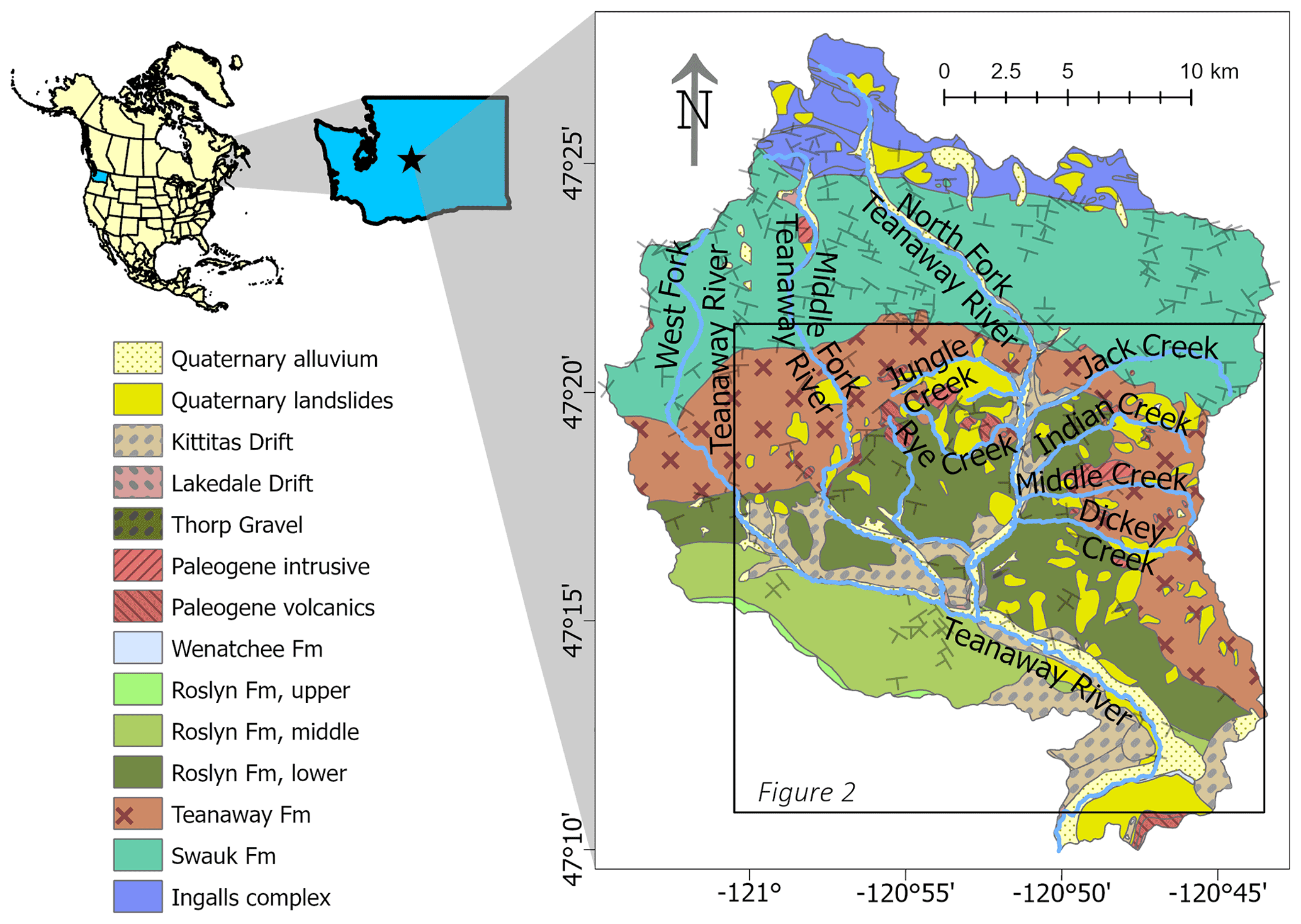
Figure 1Geologic map of the Teanaway watershed (Tabor et al., 1982) including strike and dip directions of geologic units. Upper left inset shows location of Washington State in North America, and the location of the study area (star) within Washington State. Box shows the location of Fig. 2.
The majority of rock units in the study area were deposited during the Eocene (Fig. 1). The lower Eocene Swauk Formation, composed of dark sandstone with small amounts of siltstone and conglomerate, unconformably overlies the Jurassic Ingalls Complex and is ∼4800 m thick (Tabor et al., 1984). The Swauk Formation is folded with dip directions generally to the south (Tabor et al., 1982). The middle Eocene Teanaway Formation unconformably lies on the steeply tilted Swauk Formation. The Teanaway Formation ranges from 10 to 2500 m thick and is composed of basaltic and andesitic lava flows interbedded with tuff, breccia, and feldspathic sedimentary rocks (Tabor et al., 1984). Because of its resistance to weathering, this formation forms most of the taller and more rugged peaks in the Teanaway area. Rhyolite flows from this formation have interbedded with the conformable upper Eocene Roslyn Formation and outcrop through the study area as dikes (Tabor et al., 1984). The youngest surficial rock unit, the Roslyn Formation, covers most of the lower-elevation study area. The unweathered white and weathered yellow immature sandstones were deposited conformably on the Teanaway Formation in the late Eocene (Tabor et al., 1984). The Roslyn and Teanaway formations lie relatively flat or gently tilted to the southwest compared with the Swauk Formation, and are very susceptible to erosion and sliding owing to the interbedded tuffs, paleosols, clays, and silts (NFTWA, 1996; Tabor et al., 1982).
Overlying the Eocene units are glacial and mass wasting deposits. Glacial terraces originate from the Thorp and Kittitas glaciations at 600 and 120 kyr respectively (Porter, 1976). During drift deposition, glaciers from the Cle Elum catchment to the west overtopped the dividing ridge and entered the West Fork and lower Middle and North Fork Teanaway valleys. Thorp and Kittitas moraines, composed of poorly sorted gravels and cobbles, are present at the eastern edge of the study area near the outlet of the mainstem Teanaway into the Yakima River and on the ridges surrounding the West Fork Teanaway (Porter, 1976). The Thorp drift sediments are heavily eroded and therefore less visible than the Kittitas drift sediment, which has been modified by mass wasting (Porter, 1976).
Geologic mapping has identified several Quaternary mass wasting deposits in the Roslyn and Teanaway formations (Fig. 1) and subsequent reports have focused on shallow landslides near stream banks (NFTWA, 1996). Landslides are as old as late Pliocene and are concentrated near rhyolite tuffs and a weathered surface in the Teanaway Formation, which form planes of weakness (NFTWA, 1996). Although closed depressions and ponds are visible in the lidar and suggest some recent activity, landslides are not easily distinguished in aerial photography or in the field. Lidar in 2015 and 2018 (Quantum Spatial, 2015, 2018) revealed the extent of these slides, but no studies since have quantified landslide volumes, constrained the timing or mechanism of sliding, or discussed the impact of the deep-seated landslides and earthflows on the landscape.
Our analysis focuses on the entirety of the Teanaway basin, though the majority of the earthflows are found within tributaries to the North Fork Teanaway River. To identify the temporal and spatial distribution of earthflows, we use geomorphic mapping in conjunction with a directional roughness metric to identify and relatively date earthflow activity in the Teanaway basin. Other studies (e.g., Bennett et al., 2016; Mackey and Roering, 2011) use tree and object tracking to measure earthflow velocity; we attempted to do this but found the dense vegetation and high tree growth rates prevented us from accurately matching objects between image pairs. Thus, we rely on surface roughness to give relative earthflow activity. We test the relationship between directional roughness and time since earthflow activity using a numerical model, and further constrain the relative ages using radiocarbon and sedimentation ages, which both give maximum estimates of earthflow activity.

3.1 Earthflow mapping and maximum earthflow ages
We first created a detailed earthflow map for the study region. All visually identifiable landslides within the Teanaway basin were digitized in ArcGIS from 1 m resolution lidar (Quantum Spatial, 2015, 2018) on a scale of 1:5000. Earthflows were classified from this dataset based on: hourglass shape with a wide head scarp and toe compared with a narrow transport zone, narrow width and long length of slide zone, visible levees or shear zones at the edges, and flow-like morphologies (Baum et al., 2003; Nereson and Finnegan, 2018). We mapped the edges of earthflows as the edge of shear zones next to undisturbed hillslopes, and used scarps and toe deposits to delineate the top and bottom of earthflows from surrounding hillslopes. These morphologic clues degrade over time and it becomes harder to distinguish earthflows from other mass movements. Therefore, we focus our analysis on Holocene earthflow activity when it is still possible to distinguish the characteristic earthflow morphologies.
We dated select earthflows using buried charcoal found within the earthflow toe deposits. Long residence times of buried charcoal in landslides can result in radiocarbon ages > 8000 years older than landslide activity (Struble et al., 2020); considering that earthflows can also have episodic activity, which further complicates the relationship between timing of earthflow activity and radiocarbon age, we use our charcoal ages to loosely constrain maximum earthflow activity. Maximum earthflow activity refers to a maximum estimate of how long since an individual earthflow first became active. Sampled earthflows were selected based on potential for a fresh exposure via road or stream erosion and to capture a range of activity, which we estimated by the prominence of levees and shear zones in the bare earth lidar. In the field, we removed 10–50 cm of material from the toes of earthflows exposed by stream cuts or roadcuts to find 2–5 g of charcoal (Fig. S1 in the Supplement). We collected radiocarbon samples from seven different earthflows (Table 1); one sample (8-4-20-2) did not yield enough carbon material to date. The samples were sent to the Center for Applied Isotope Studies (CAIS) lab at the University of Georgia and were dated using Accelerated Mass Spectrometry (AMS); dates were calibrated to calendar years using Intcal20 (Reimer et al., 2020).
In three cases where earthflows dammed the valley and formed lakes, we estimated the onset of valley blockage, and thus an estimate for when earthflow activity began, by using the sedimentation age of the lake. We reconstructed a pre-earthflow valley bottom using the techniques in Struble et al. (2020). We estimated the valley bottom elevation under the lakes using the average valley slope of surrounding un-dammed valleys. This valley floor estimate is interpolated in the geographic information system (GIS) with the lake perimeter elevation to form an estimated lake bottom topography. The bottom topography is subtracted from the lidar surface elevation to estimate the sedimentation volume post-earthflow. We used nearby mid-Holocene 10Be denudation rates of 0.08 and 0.17 mm yr−1 (Moon et al., 2011) from neighboring basins with similar mean annual precipitation and glaciation. We multiplied the denudation rates by upstream contributing area for each lake to give a volumetric estimate of sediment delivery per year. The lake sedimentation volume is divided by this rate to estimate the years necessary to fill each lake. We repeat this process with the upper and lower denudation bounds to give a range of plausible sedimentation ages, which approximate when the earthflow dammed the creek. Earthflow activity may continue after lake formation; thus, these sedimentation ages do not necessarily represent the most recent earthflow activity.
3.2 Estimating earthflow activity using flow directional surface roughness
To relatively date earthflow activity, we created a surface roughness age calibration model similar to that used to date rotational slides in Washington State (LaHusen et al., 2016; Booth et al., 2017). Active earthflows have a unidirectional flow morphology that gradually diffuses to less directional roughness as activity ceases, in contrast to rotational slides which start with uneven roughness in all directions. To account for the unique flow morphology of earthflows, we used a flow directional median absolute differences (MAD) index (Trevisani and Rocca, 2015). MAD is a bivariate geostatistical index that analyzes residual elevations between paired locations in a digital elevation model (DEM) (Trevisani and Cavalli, 2016). MAD results in a roughness index for each direction (N–S, E–W, NE–SW, and NW–SE) across each raster cell in the study area. Using surface flow directions derived from the DEM surface, these directional roughnesses are filtered to correspond to the flow direction; e.g., if the surface flow direction is N–S, then only the N–S roughness is used (Trevisani and Cavalli, 2016). A high MAD value represents topographic roughness in the direction of flow, whereas a low MAD represents relatively smooth regions.
MAD is calculated using the residual roughness to filter out large-scale topographic variations; we first smoothed the 1 m DEM over a 3×3 window followed by a 5×5 window (Trevisani and Cavalli, 2016) and subtracted the smoothed DEM from the original DEM to obtain a raster of residual roughness elements (Figs. S2 and S3). The MAD index (https://github.com/cageo/Trevisani-2015, last access: 16 June 2021) was run with this residual raster and calculated the directional roughness over an 8 m radius window. We chose this window so that we examine a similar spatial scale to the 15×15 window used by LaHusen et al. (2016). We calculated flow direction across the smoothed DEM and created a raster with the MAD values in the direction of flow for each cell. Finally, we used Zonal Statistics to calculate the standard deviation of the directional roughness (MADstd) for each earthflow; from our diffusion model simulations (see below), MADstd had the highest correlation with age (R2=0.98).
The MADstd relative dating method rests on the assumption that earthflow MADstd will decrease with time since last earthflow activity owing to soil diffusion. In order to test this assumption, we simulated landscape diffusion on a recent earthflow and calculated MADstd through time; if our assumption is correct, MADstd should decrease with simulation time. We extracted elevations from an earthflow along Jungle Creek, where we obtained radiocarbon sample 8-1-20-1 (Fig. 2, Table 1). We chose this earthflow because it has clear flow lines and blocks the majority of the stream valley with an outlet eroded through. This suggests the earthflow has been active recently to block the valley. We applied two-dimensional diffusion to the earthflow surface, based on Eq. (1):
where dz is the change in elevation, dt is the timestep, and dx is the spatial resolution. The diffusion rate, K, is estimated as 0.002 m2 yr−1 based on regions in a similar climate (Martin, 2000), although we varied the diffusion rate as low as 0.0002 m2/yr for landscapes experiencing creep (Martin, 2000). We also ran the diffusion model with and without stream erosion. Stream erosion is represented by Eq. (2):
where A is the upstream contributing drainage area, S is slope, and Ksp, m, and n are empirical coefficients related to drainage basin geometry, rock erodibility, channel hydraulics, and climate (Braun and Willett, 2013). The values of m and n are set at 0.5 and 1 respectively, based on common values for mountain streams (Braun and Willett, 2013), and Ksp is estimated at from empirical relationships between average denudation (Moon et al., 2011), A, and S along Jungle Creek. We ran the diffusion model for 10 kyr and calculated MAD every 2 kyr.
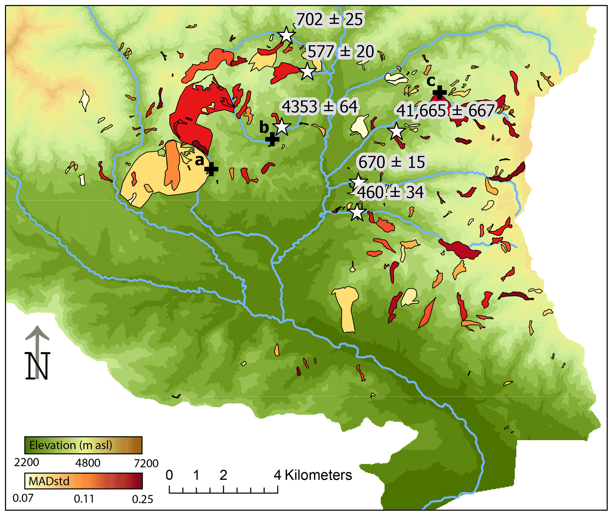
Figure 2Earthflows mapped in the study area; earthflows are colored by their MADstd value. Radiocarbon locations and dates, in calibrated yr BP, are shown with white stars. Black crosses indicate locations of earthflow-dammed lakes where sedimentation ages are derived: (a) unnamed creek; (b) Rye Creek; and (c) Indian Creek. Extent of region is shown in Fig. 1. Background elevation data from Quantum Spatial (2015, 2018).
3.3 Valley width
To examine the influence of landslides on habitat, we measured valley width along the tributaries of the North Fork Teanaway. Valley width typically increases with increasing drainage area in a power law relationship of form:
where Wv is valley width, a and b are empirical parameters, and A is upstream drainage area. In the Washington and Oregon Coast Ranges within similar sedimentary rocks to the Roslyn Formation but in a wetter climate, a is 67 and b is 0.34 (Schanz and Montgomery, 2016) for a landscape lacking deep-seated landslides or earthflows. Similar values for b are found across the tectonically quiescent Appalachian Plateau, USA (Clubb et al., 2022).
In order to isolate the effect of earthflows on valley width, we focus on tributary valleys of the North Fork. The mainstem and three forks of the Teanaway all have wide valleys that are unaffected by earthflows. In contrast, the tributary valleys of the North Fork are altered by earthflows. We extracted valley width from Jungle, Rye, Dickey, Middle, Indian, Jack, and an unnamed creek (Fig. 1) by defining the valley floor as being less than 5 % slope. We used an automated process in ArcGIS to extract a valley centerline, create transects every 100 m, and measure valley width as the width of the transect line within the 5 % valley slope.
We present the results of earthflow mapping and dating below. In order to verify the relative dating method, we first present earthflow mapping, valley width, and maximum age estimate results. We then use those results and the diffusion simulations to test how well the MADstd relative dating works. Finally, we conclude with a basin-wide perspective on the timing of earthflows based on MADstd values.
4.1 Earthflow mapping
We mapped 187 earthflows in the lower Teanaway basin (Fig. 2). Earthflows range in size from 1076 m2 to earthflow complexes 4×10⁶ m2 with median sizes of 28 547 m2. Mapped earthflows are mostly all north of the mainstem and Middle Fork of the Teanaway River, with the exception of eight small earthflows south of the Main Fork. The southern edge of the earthflow area appears to be bound by the extent of Pleistocene glaciation (Fig. 1); perhaps glaciation removed pre-existing earthflows, or the muted topography from glacial erosion is less prone to mass movement. To the north, the earthflow domain is bound by the start of the Swauk Formation, which has little to no mappable landslides in it.
Earthflows spatially cluster in the Teanaway and lower Roslyn formations. Just over half (51 %) of mapped earthflows are in the Teanaway Formation, which is composed of basalt and rhyolite interbedded flows and conformably grades upwards into the lower Roslyn Formation, in which 42 % of earthflows are found. The remaining 7 % are split between the Swauk and middle Roslyn Formations.
We extracted slope and aspect for each earthflow. The slope distribution, measured based on the smoothed 1 m lidar, was similar between earthflows and intact hillslopes of the Lower and Middle Roslyn Formations with modal slopes of 10 to 15∘. The average earthflow aspect shows strong preference for the southwest quadrant, with 45 % of earthflows (Fig. 3). The northwest and southeast quadrants were similarly populated with 20 % and 21 %, respectively, whereas the remaining earthflows are found in the northeast quadrant.

Figure 3Average earthflow aspect, binned by 10 degrees. Contours indicate number of earthflows in each bin.
4.2 Valley width
Valley width generally increases with drainage area for the seven tributaries we examined, although the increase is not consistent (Fig. 4). Jungle Creek has its narrowest width, equivalent to the channel width, halfway up the valley where a high MADstd earthflow pinches the valley. The valley width immediately upstream is 100 m wide, comparable with the widest part of the valley at the mouth of Jungle Creek. Similarly, Rye Creek's valley is pinched to the channel width at 2 km upstream (drainage area = 7.5×10⁶ m2) and widens immediately upstream to the widest values noted along the tributary. Similar trends of narrowed valleys with wider sections immediately upstream are seen in the other tributaries, although the trends are less strong. Rye, Middle, Indian, and the unnamed creek are confined by earthflows in the upper 1–2 km; these earthflows form the valley walls and bottom and constrain the valley width to the active channel width.
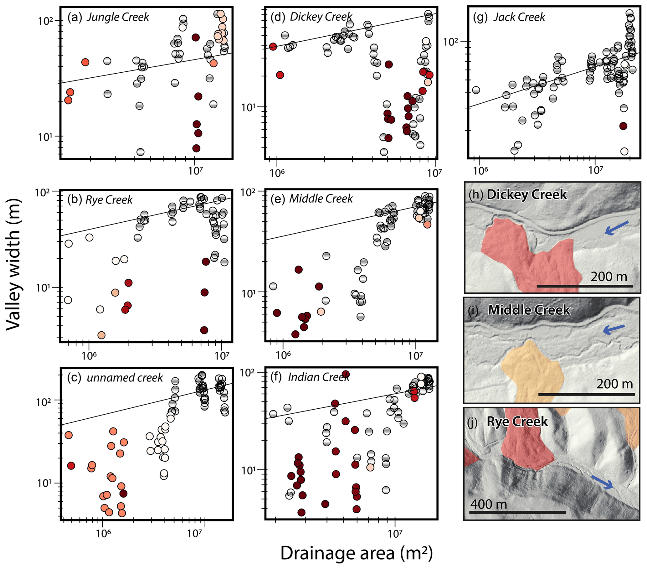
Figure 4Valley width of the North Fork tributaries compared with upstream contributing drainage area (a–g). Black lines show a power law relationship with exponent 0.3 (Schanz and Montgomery, 2016; Clubb et al., 2022). Tributaries are arranged counterclockwise from the northwest (see Fig. 1 for locations). Colored circles indicate valley width measurements where one valley wall is an earthflow; colors reflect MADstd relative to earthflows within that tributary in which red are high MADstd and light pink are low MADstd. Panels (h)–(j) show examples of earthflows interacting with valley bottoms; earthflow color corresponds to MADstd value using the same color scheme as panels (a)–(g). Blue arrows show the direction of the water flow.
4.3 Maximum earthflow ages
Age results from radiocarbon dating range from 370 to 36 750 carbon-14 years before present, or 460±34 to 41 665±237 calibrated years before present (yr BP) (Table 1, Fig. 5). Samples were taken from the toe of earthflows, representing charcoal that was originally deposited in regolith and then transported through earthflow movement. Thus, the age given by radiocarbon dating is a measure of (1) the inherited age of the charcoal, (2) regolith development, (3) earthflow transport, and (4) deposition at the earthflow toe. We cannot use our ages to directly date the last earthflow activity, but it does provide a maximum estimate of earthflow age.
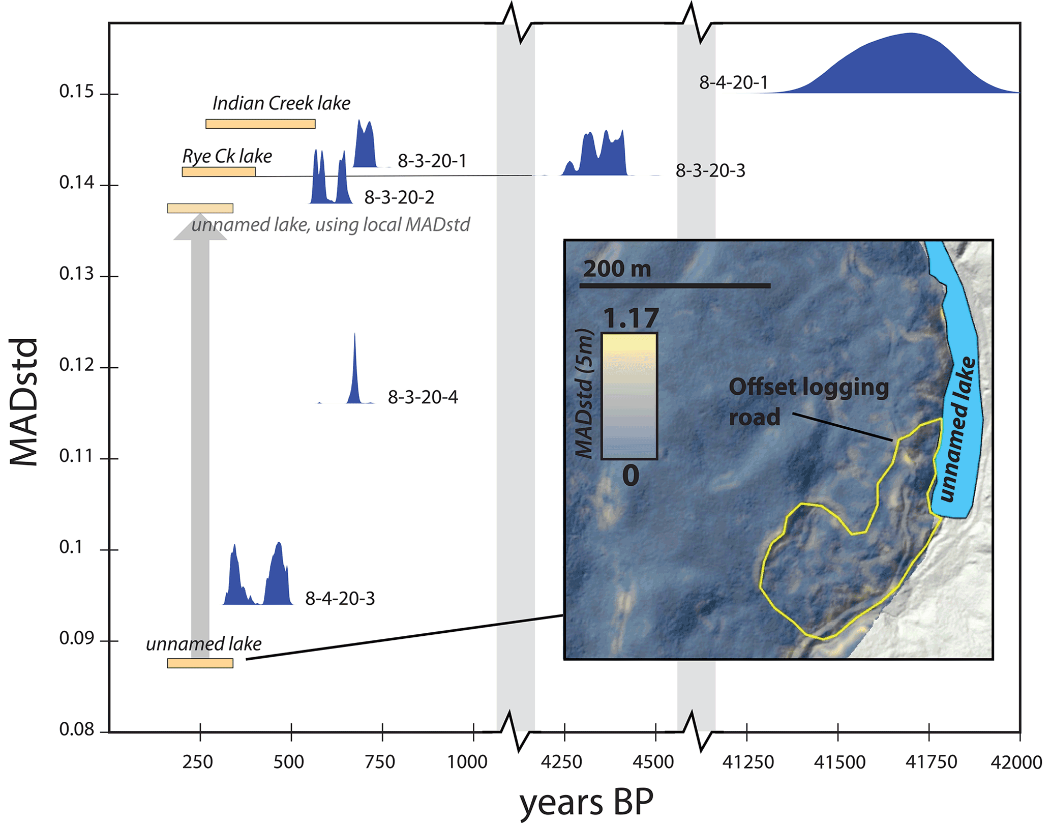
Figure 5Comparison of maximum age estimates and MADstd values. Range of maximum earthflow ages from lake sedimentation are shown as orange bars and radiocarbon ages are shown with blue probability distribution functions. Inset shows the MADstd values calculated with a 5 m moving window for the earthflow complex creating the unnamed lake. Note the relatively low MADstd in blue despite dense Pinus ponderosa forest covering the earthflow surface. Yellow outline shows a possible re-activation of part of the complex, which raises the MADstd associated with lake formation from 0.087 to 0.137.
Based on a range of denudation rates of 0.08 to 0.17 mm yr−1, the lake formed along Indian Creek (Fig. 2) took approximately 267 to 567 years to fill to the current level (Fig. 5), indicating that the earthflow has been constricting Indian Creek for at least that long. The lake along Rye Creek, formed just upstream of earthflow carbon site 8-3-20-3, took between 204 and 433 years to fill with sediment to the modern level, and the lake along the unnamed creek took approximately 159 to 337 years to fill.
The ages we derived from sedimentation rates and lake volume do not directly date earthflow activity, although the relationship is more complex than the radiocarbon ages. The lake itself formed when the earthflow initially dammed the valley, and so represents a maximum age – or a near maximum age if earthflow velocity was slower and did not immediately dam the channel. However, all lakes are currently filled with sediment and an outlet stream has eroded through the damming earthflow, which indicates that the sedimentation age is a minimum estimate of the lake's age. Based on the observation that the outlet stream is still forming a knickpoint in the earthflow and has not yet incised through the lake fill, we believe that the sedimentation age is close to the age of the lake and thus these ages more closely estimate the maximum earthflow age.
We were able to get a radiocarbon age and a sedimentation age for one earthflow: the Rye Creek earthflow was dated with charcoal to 4353 yr BP but has a sedimentation age of 204 to 433 years. These ages indicate upwards of 4000 years of residence time for charcoal in the earthflow, similar to values found for rotational landslides in the Oregon Coast Range (Struble et al., 2020), and a maximum estimate of earthflow activity to approximately 204 to 433 years ago. The other earthflows creating lakes are similarly young, with maximum ages in the last 500 years; radiocarbon ages support relatively recent earthflow activity with maximum age estimates of less than 1000 years for four of the six dated earthflows.
4.4 Verification of MADstd relative dating
Simulated diffusion verified our assumption that MADstd decreases with time since earthflow activity. The Jungle Creek earthflow shows a strong linear relationship between MADstd and earthflow age (Fig. 6) with an R2 fit of >0.98 for all four hillslope diffusion values tested. When simulations were run with stream erosion, resulting MADstd values were very similar, with less than 5 % difference in values and a median difference of 0.2 %. Therefore, whether stream erosion is considered or not is negligible to the MADstd value. The linear decrease in MADstd values with time supports our initial theory that as earthflows stop moving, the directional roughness becomes more similar across the earthflow surface. Soil diffusion creates a more multi-directional surface with lower variation in flow directional roughness. When earthflows are active, orthogonal flow off the flow features and scarps creates a highly variable MAD and thus a high MADstd.
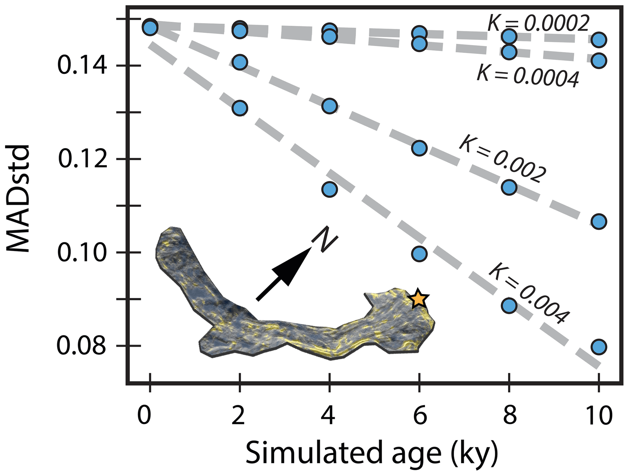
Figure 6MADstd values for simulated diffusion across the Jungle Creek earthflow. Inset image shows the Jungle Creek slide with modern (simulation time = 0) MAD values where yellow are high directional MAD and blue are low. Star shows location of sample 8-3-20-1. For all diffusion values, linear regressions give an R2 of >0.98.
Although our simulations give equations relating to age and MADstd, we do not apply this equation to the study area because the relationship is highly dependent on the soil diffusion value and on earthflow velocity, which would affect the relative strength of diffusive versus advective processes. We do not know the site-specific diffusion rate, and even slight differences between K=0.0002 and 0.0004 give widely different age estimates (Fig. 6). We also do not know how the diffusion rate changed over the late Quaternary in our study area. However, we can assume that the diffusion rate and associated variations are similar across our study area, where climatic and biotic forcings are relatively uniform and earthflow source lithology is either lower Roslyn or Teanaway formation. Thus, we should be able to use MADstd to relatively date earthflow activity.
When we apply the MADstd metric to mapped earthflows (Fig. 2), topographic relationships support the relative dating technique (Fig. 7). In our study area, there are 22 instances of earthflows clearly overlapping with another, in which morphologic clues can be used to relatively date them. Of these, 16 had MADstd values consistent with the cross-cutting relationship where the on-lapping earthflow had higher MADstd values than the underlying earthflow. In cases where the MADstd gave incorrect relative ages, five were on earthflow complexes. MADstd appears to not work as well across large earthflow complexes where there is more heterogeneity in activity and less defined flow lines and scarps. If we disregard earthflow complexes, then only one of the 17 cross-cutting relationships is not consistent with the relative MADstd values.

Figure 7(a) Cross-cutting relationships compared with MADstd relative age relationships and (b–d) examples of cross-cutting relationships underlain by a lidar hillshade (Quantum Spatial, 2015, 2018). (b) Two examples where the higher MADstd earthflow topographically truncates two lower MADstd earthflows. (c) An example where the MADstd relative dating does not work, in which the cross-cutting earthflow has a lower MADstd than the earthflow complex it sits within. (d) An example where the toe of a lower MADstd earthflow onlaps a higher MADstd earthflow, indicating a mismatch between MADstd and topography. Numbers indicate the MADstd value for each earthflow, which is also reflected by the earthflow color, using the same color scheme as Fig. 2.
Valley bottom impingement also supports the MADstd relative ages. Active earthflows are more likely to block tributary valleys in contrast to older, less active earthflows whose deposits can be eroded by the stream to re-form a wide valley. Earthflows that completely block valleys, or narrow valleys to the channel width, have higher MADstd values than earthflows that only partially block valleys (Fig. 4h–j). Earthflows with low MADstd values are near the regression line for non-landslide terrain, suggesting that their toes might have been eroded to the valley walls (Fig. 4). One outlier to this is the 4–6 km along Rye Creek and the unnamed creek (Fig. 4b and c) with a low MADstd but strong effect on valley width. Both of these earthflows are large earthflow complexes (3–4 km2) and the MADstd value of the entire complex may not represent the locally active portions that affect the two creeks.
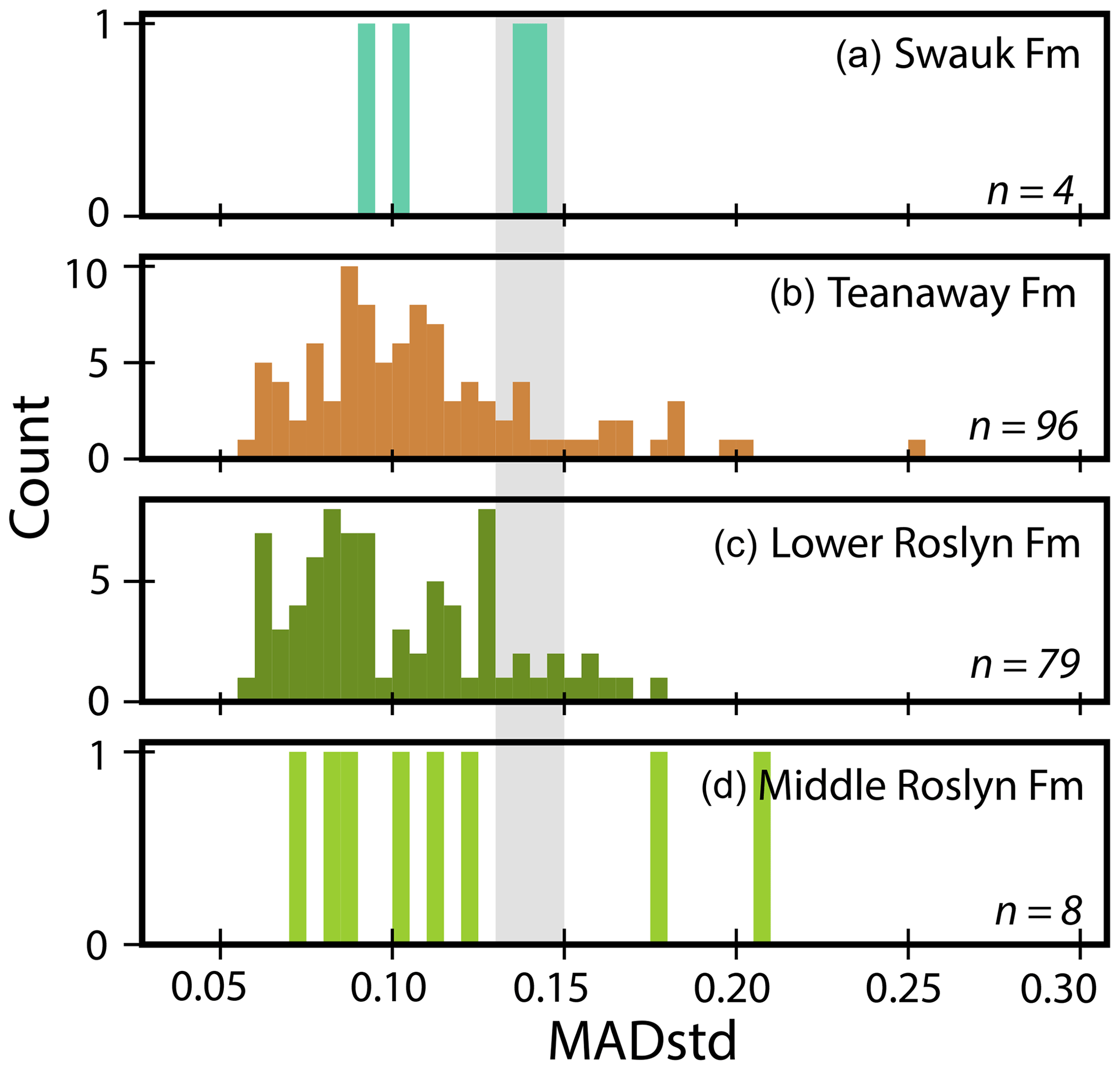
Figure 8Distribution of MADstd values by lithology, binned by 0.05. Gray bars show the MADstd range 0.13 to 0.15 that is associated with recently active earthflows.
Although MADstd appears to work to relatively date earthflows across the study area, comparing lake sedimentation ages and MADstd indicates that earthflows active at a similar time may display a range of MADstd values. Lakes along Rye and Indian Creek have sedimentation ages of 204 to 433 and 267 to 567 years, respectively, with MADstd values of associated valley-blocking earthflows of 0.141 and 0.146 (Fig. 5). Given the error in sedimentation ages, we consider these lakes to have formed at approximately the same time, thus indicating that MADstd values can range by at least 0.005 for earthflows with similar activity history.
The sedimentation age for the lake along the unnamed creek is an outlier, with the youngest range of sedimentation ages (159 to 337 years) yet the lowest MADstd of 0.087, which represents the least active earthflow of the three lakes studied. The 0.087 value comes from a large earthflow complex that borders the western and southern edge of the lake. When MADstd is calculated using a moving window of 5 m, variations in MADstd across the earthflow complex become clear (Fig. 5, inset). In particular, a higher MADstd region can be identified at the base of the lake, where a sharper headscarp and an offset logging road indicate reactivation of this part of the earthflow complex. The MADstd of the reactivated portion is 0.137, much higher than the 0.087 value for the earthflow complex as a whole. When the new value is used, we see that the three lakes cluster in a range of MADstd values of 0.137 to 0.146 with an age of approximately 250–500 years. Therefore, we conclude that earthflows active in the last few hundred years may have a range of MADstd of 0.137 to 0.146. When relatively dating earthflow activity, we should use MADstd differences of >0.01 to differentiate separate periods of earthflow activity.
4.5 Relative earthflow activity
Now that constraints on MADstd usage are determined, we analyze patterns in relative earthflow age by underlying lithology. Soil diffusion is the primary control on the relationship between MADstd and earthflow activity (Fig. 6); diffusion is set by climate (Sweeney et al., 2015) and lithology (Johnstone and Hilley, 2015), which determine the rate of soil movement as well as soil thickness. The study area experiences similar climate, and so we can compare earthflows within each lithologic unit with contrast relative earthflow activity.
Only five and eight earthflows are sourced in the Swauk or Middle Roslyn formations, respectively, and MADstd values range from 0.07 to 0.21 (Fig. 8). The majority of earthflows (n=96) are underlain by the volcanic Teanaway Formation. MADstd values are clustered around 0.10, with a small frequency peak near 0.17. Unlike the mostly unimodal distribution in the Teanaway Formation, earthflows in the lower Roslyn Formation have a bimodal MADstd distribution with peaks at 0.08 and 0.13.
Absolute ages suggest that earthflows active in the last few hundred years might have MADstd values of 0.13 to 0.15, approximately (Fig. 5), and that differences of >0.01 MADstd are necessary to distinguish between relative earthflow ages. Based on this, the earthflows underlain by the Teanaway Formation are mostly inactive but do contain some earthflows that have been active in the last few hundred years; 24 (25 %) earthflows have MADstd of >0.13. For earthflows underlain by the Roslyn Formation, a similar percentage were likely active in the last few hundred years, with 20 (25 %) earthflows with a MADstd of >0.13.
That the MADstd values for the lower Roslyn Formation are bimodal indicates that the prevalence of active earthflows with MADstd of >0.13 is unlikely to be due to a preservation bias, nor to constant earthflow activity. Instead, the sharp break between active earthflows and the cluster of older earthflows around 0.08 MADstd suggests a history of: initial earthflow activity, followed by a cessation in which soil diffusion acted across earthflows, then re-activation or new earthflow formation of 25 % of the earthflows in the study area.
5.1 Drivers of earthflow motion
Our aspect analysis showed a strong preference for earthflows to be oriented toward the southwest quadrangle (Fig. 3), and we hypothesize that this might reflect a bedding plane control of earthflow location. The Roslyn and Teanaway Formations are gently dipping to the southwest (Fig. 1) with dip angles ranging from 10 to 30∘ (Tabor et al., 1982), comparable with the modal and median earthflow slopes. There is some variability in the bedding orientation as the Teanaway and Roslyn formations curve to the west, but only 8.5 % of earthflows by area are located in this southeast-dipping region. Southeast aspects account for 21 % of mapped earthflows; this mismatch implies that not all earthflows are directly aligned to underlying bedding planes. Possibly, southerly aspects could be preferential owing to vegetation and evaporation conditions that affects hillslope stabilization. However, the hillslopes in our study area are uniformly Pinus ponderosa-dominated forest. The preponderance of SW facing earthflows thus indicates that most earthflows are lithologically controlled. Since the Roslyn and Teanaway are conformable, the bedding plane orientation also reflects the mid-Eocene landscape surface, and therefore the orientation of paleosols within the two units. Previous work has noted that paleosols and volcanic flows interspersed in the Teanaway and Roslyn formations form planes of weakness for landslides (NFTWA, 1996). That our observed slopes and aspects match the bedding orientation supports this finding and indicates that the bedding provides a first-hand control of the orientation of earthflows in the Teanaway basin.
Further support for a lithologic control is the prevalence of earthflows in the Teanaway and lower Roslyn Formations, with 94 % of mapped earthflows in these two units, which make up 32.7 % of the study area. The southern edge of mapped earthflows does align with the extent of Pleistocene glaciations, which overtopped the western drainage boundary and flowed in through the West Fork Teanaway. Although earthflows likely postdate the 120 kyr glaciation, the muted topography resulting from glacial erosion may be less prone to earthflows. The glacial extent overlaps both the middle and lower Roslyn Formation (Fig. 2), and earthflows in the lower Roslyn Formation stop at the low relief topography left by glacial erosion. Thus, glacial erosion, in addition to underlying lithology, appears to control the extent of earthflow activity. At the southern edges of the study area, glacial erosion is minimal and topographic relief increases. However, only eight small earthflows were mapped in this region, which is underlain by the middle and upper Roslyn Formations. Although conformable, the middle and upper Roslyn Formation members lack rhyolite interbeds and are finer grained in comparison with the lower member (Tabor et al., 1984). Likely, the interbedded rhyolite allows planes of weakness to form (NFTWA, 1996) that promote earthflow formation.
Our absolute and relative ages indicate that approximately 25 % (n=46) of the mapped earthflows were active within the last few hundred years; however, we do not have strong age control for the remaining 141 earthflows. Earthflow activity often correlates with climate (Bennett et al., 2016), with wetter periods driving earthflow motion (Baum et al., 2003) and drier periods creating desiccation cracks that prime the landscape for deep water infiltration (McSaveney and Griffiths, 1987). The last few hundred years in the Teanaway basin were climatically characterized by the Little Ice Age, which caused about 1 ∘C cooler conditions (Graumlich and Brubaker, 1986). This temperature change is unlikely to significantly alter weathering rates and regolith production (Marshall et al., 2015; Schanz et al., 2019), and precipitation rates remained low. However, human modification since 1890 may have contributed to earthflow activity. Starting ca. 1890, large-scale deforestation and road building began (Kittitas County Centennial Committee, 1989), which would decrease evapotranspiration and root strength, leading to greater water infiltration and weaker soil cohesion; conditions that promote earthflow movement. Similar patterns are seen in the Waipaoa River basin, New Zealand, where deforestation in the last 200 years has resulted in mass movements and increased sediment loads (Cerovski-Darriau and Roering, 2016).
5.2 Landscape disturbance
Earthflows in the Teanaway basin alter valley bottom topography and hillslope erosion rates, which affects habitat zones and Holocene denudation rates. In the Teanaway forks and mainstem, no earthflows encroach on the valley bottoms, but all of the North Fork tributaries examined in Fig. 4 initiate on an earthflow or earthflow complex, with the exception of Jack and Dickey creeks. Only a relatively small number (10 of 187) of mapped earthflows in the North Fork tributaries are in direct contact with streams; these earthflows range in size from a large earthflow complex of 4 km2 to smaller flows of 14 000 m2 and show mostly recent (<200 years) activity.
Increased sediment flux from earthflows appears to be mostly fine sediment; grain size surveys indicate high amounts of fine sediment and moderate coarse sediment loads in the North Fork tributaries with no significant difference between tributaries draining Teanaway and lower Roslyn formations, despite a rock strength difference between the basalt and friable sandstone (NFTWA, 1996). In a similar sandstone formation, Fratkin et al. (2020) found significant variation in surface and subsurface grain size when compared with adjacent tributaries draining basalt; most bedload in their study area was delivered by debris flows and landslides. However, earthflows tend to incorporate highly weathered material and regolith; in the Eel River, 90 % of earthflow colluvium is smaller than 76 mm (Mackey and Roering, 2011). Field observations in the Teanaway at earthflow toes and exposed surfaces were of sand and silt size fractions, with a few small gravels (Fig. S1), even at radiocarbon site 8-4-20-2, which had insufficient carbon to produce an age but is from an earthflow sourced entirely from the Teanaway Formation basalt. Thus, the abundant fine sediment and lack of significant grain size difference between tributaries in the Teanaway and lower Roslyn formation may reflect large sediment contributions from earthflows, which preferentially transport weathered regolith.
These effects on sediment flux and valley width are likely to disturb in-stream habitat. Heightened fine sediment delivery can clog pore spaces in spawning gravels; however, channel slopes in the Teanaway basin are high and sufficient to quickly transport sands and finer material downstream (NFTWA, 1996; Schanz et al., 2019). Floodplain habitat is reduced where earthflows narrow the valley (Fig. 4), although valley widths are abnormally large just upstream of earthflows in Jungle, Rye, and Dickey creeks. Valley width is a key landscape characteristic for salmon habitat (Burnett et al., 2007) and wider valleys are often associated with heterogeneous channel features (Montgomery and Buffington, 1997) and flood refuge habitat (May et al., 2013). That Teanaway earthflows can create heterogeneity in valley widths implies that they exert a direct influence on riparian habitat.
5.3 MADstd as a relative dating tool
Our lake sedimentation ages showed very little relationship between MADstd and earthflow activity for recent earthflows; however, this finding is consistent with those of other studies of landslide surface roughness. Comparing three surface roughness metrics on landslides spanning ∼200 years of activity, Goetz et al. (2014) found no relationship between surface roughness and age. Booth et al. (2017) suggest that surface roughness might be more appropriately used to distinguish landslide ages on a scale of thousands of years. Thus, the limitations of MADstd are similar to those of other surface roughness metrics in that we cannot distinguish relative earthflow activity of <200 years.
Yet, MADstd is able to identify flow features and differentiate between forest terrain, which gives it an advantage over some other roughness metrics. The original flow directional MAD metric picks up flow features such as scarps, debris flows, and channels that are missed by isotropic roughness metrics (Trevisani and Cavalli, 2016). In the case of earthflows, high and low flow directional MAD values are associated with the strong lineations; as flow follows the crests and hollows, the >1 m lineations also direct flow orthogonal to crests (Fig. 6, inset). By taking the standard deviation, we can highlight the parallel and orthogonal flow that is characteristic of >1 m scale lineations; however, it is important to note that this method would not work if the elevation model resolution is greater than the lineation scale. Compared with other metrics applied to landslides, the MADstd includes a flow directional roughness and detrends the data, both of which have been found to improve landslide identification accuracy (Berti et al., 2013; McKean and Roering, 2004). Previously used surface roughness metrics often have trouble capturing the top of earthflows and differentiating between rough, forested terrain and landslide roughness (Berti et al., 2013). When the MADstd is calculated over a moving 5 m radius window, rather than over a single earthflow, forested hillslopes are clearly delineated from earthflows. The roughness elements from trees are isotropic and give MADstd values near zero (Fig. 5, inset). The scarp, flowlines, and toe produce strong lineations in the landscape that light up in the MADstd plots, owing to the parallel and orthogonal flow over the 1 m DEM. Even smaller earthflows, of approximately 3600 m2, are identified with the 5 m moving window MADstd. This advantage over previous, isotropic methods of calculating surface roughness and identifying landslides indicates that MADstd is an appropriate method for use in identifying and mapping earthflows, although we caution that the DEM resolution size must be less than the scale of earthflow lineations.
Further, the decay of MADstd with age shows potential, particularly if it can be used as an absolute age when combined with other dating methods. As time since earthflow activity increases, MADstd decreases in a strongly correlated (R2>0.98) linear relationship. Any error in the linear relationship remains similar despite the time frame considered. In contrast, other surface roughness metrics such as standard deviation of slope have an exponential relationship with landslide age. When calibrated to absolute dating, exponential relationships can result in errors up to ±1 kyr for landslides that are 10 kyr old (LaHusen et al., 2016). Although we were unable to convert the MADstd relationship to an absolute age relationship for the Teanaway, the MADstd roughness metric has potential as a more precise method of dating older mass movements (∼10 kyr or greater).
To examine controls on earthflow activity and resulting topographic disturbance in the Teanaway basin, we mapped and dated earthflows using 1 m lidar and a new relative dating method that relies on flow directional surface roughness. The MADstd metric appears well-suited to identifying and relatively dating earthflows, as it picks up linear roughness elements such as lateral shear zones and levees, and is able to ignore the influence of dense vegetation on the elevation model. This is particularly useful for densely vegetated areas, where other roughness metrics have difficulty and where application of object tracking is problematic. In addition to MADstd relative ages, we used radiocarbon and sedimentation ages to provide a few constraining absolute ages; these ages indicate that 25 % of earthflows in the Teanaway basin were active in the last few hundred years. Nearly all earthflows (94 %) occur in the Teanaway and lower Roslyn Formations, which contain interbedded basalt and rhyolite flows along with paleosols and coarse sandstone. Slide aspect and slope roughly follow the orientation of the paleosol and volcanic flow dip angles, suggesting a strong lithologic control on earthflow location and orientation. Most tributaries in the Teanaway initiate on earthflow complexes, and experience valley width changes due to earthflow damming and associated upstream widening. Despite some variability in source lithology, the selective transport of regolith and weathered material by earthflows results in delivery of fine sediments. Although this fine sediment poses a potential hazard for instream habitat, stream power is sufficient to transport it downstream; therefore, the largest habitat disturbance provided by the earthflows is heterogeneity in valley width.
The diffusion simulation code and input files can be accessed at: https://doi.org/10.5281/zenodo.6871538 (Schanz, 2022). Landslide information and dates are available at: https://doi.org/10.5281/zenodo.5885660 (Schanz and Colee, 2021).
The supplement related to this article is available online at: https://doi.org/10.5194/esurf-10-761-2022-supplement.
SAS conceptualized the study, SAS and APC contributed equally to study design and methodology. APC and SAS acquired funding for the study. SAS wrote the paper with contributions from APC.
The contact author has declared that neither of the authors has any competing interests.
Publisher's note: Copernicus Publications remains neutral with regard to jurisdictional claims in published maps and institutional affiliations.
We thank Matt Cooney for GIS help, and Jamie and Catharine Colee for help in the field. Field work was conducted on the traditional territory of the Yakama and Wenatchi People. Suggestions from Oliver Francis and two anonymous referees greatly improved the manuscript.
This research has been supported by the Patricia J Buster grant from the Colorado College Geology Department.
This paper was edited by Lina Polvi Sjöberg and reviewed by Oliver Francis and two anonymous referees.
Abbe, T. B. and Montgomery, D. R.: Large woody debris jams, channel hydraulics and habitat formation in large rivers, Regul. River., 12, 201–221, https://doi.org/10.1002/(SICI)1099-1646(199603)12:2/3<201::AID-RRR390>3.0.CO;2-A, 1996.
Agee, J. K.: Fire and weather disturbances in terrestrial ecosystems of the eastern Cascades, US Department of Agriculture, Pacific Northwest Research Station, https://www.fs.fed.us/pnw/pubs/pnw_gtr320.pdf (last access: 6 July 2018), 1994.
Agee, J. K.: Fire Ecology of Pacific Northwest Forests, Island Press, 513 pp., ISBN 978-1-61091-378-2, 1996.
Baum, R., Savage, W., and Wasowski, J.: Mechanics of earth flows, in: Proc. Int. Conf. FLOWS, Sorrento, Italy, 2003.
Beeson, H. W., Flitcroft, R. L., Fonstad, M. A., and Roering, J. J.: Deep-Seated Landslides Drive Variability in Valley Width and Increase Connectivity of Salmon Habitat in the Oregon Coast Range, J. Am. Water Resour. Assoc., 54, 1325–1340, https://doi.org/10.1111/1752-1688.12693, 2018.
Bennett, G. L., Roering, J. J., Mackey, B. H., Handwerger, A. L., Schmidt, D. A., and Guillod, B. P.: Historic drought puts the brakes on earthflows in Northern California, Geophys. Res. Lett., 43, 5725–5731, https://doi.org/10.1002/2016GL068378, 2016.
Berti, M., Corsini, A., and Daehne, A.: Comparative analysis of surface roughness algorithms for the identification of active landslides, Geomorphology, 182, 1–18, https://doi.org/10.1016/j.geomorph.2012.10.022, 2013.
Booth, A. M., LaHusen, S. R., Duvall, A. R., and Montgomery, D. R.: Holocene history of deep-seated landsliding in the North Fork Stillaguamish River valley from surface roughness analysis, radiocarbon dating, and numerical landscape evolution modeling, J. Geophys. Res.-Earch, 122, 456–472, https://doi.org/10.1002/2016JF003934, 2017.
Braun, J. and Willett, S. D.: A very efficient O(n), implicit and parallel method to solve the stream power equation governing fluvial incision and landscape evolution, Geomorphology, 180–181, 170–179, https://doi.org/10.1016/j.geomorph.2012.10.008, 2013.
Burnett, K. M., Reeves, G. H., Miller, D. J., Clarke, S., Vance-Borland, K., and Christiansen, K.: Distribution of Salmon-Habitat Potential Relative to Landscape Characteristics and Implications for Conservation, Ecol. Appl., 17, 66–80, https://doi.org/10.1890/1051-0761(2007)017[0066:DOSPRT]2.0.CO;2, 2007.
Cerovski-Darriau, C. and Roering, J. J.: Influence of anthropogenic land-use change on hillslope erosion in the Waipaoa River Basin, New Zealand, Earth Surf. Proc. Land., 41, 2167–2176, https://doi.org/10.1002/esp.3969, 2016.
Cle Elum Tribune: Cle Elum Tribune, 20 March 1891, p. 4, Washington State, USA, 1891.
Clubb, F. J., Weir, E. F., and Mudd, S. M.: Continuous measurements of valley floor width in mountainous landscapes, Earth Surf. Dynam., 10, 437–456, https://doi.org/10.5194/esurf-10-437-2022, 2022.
Coe, J. A.: Regional moisture balance control of landslide motion: Implications for landslide forecasting in a changing climate, Geology, 40, 323–326, https://doi.org/10.1130/G32897.1, 2012.
Fratkin, M. M., Segura, C., and Bywater-Reyes, S.: The influence of lithology on channel geometry and bed sediment organization in mountainous hillslope-coupled streams, Earth Surf. Proc. Land., 45, 2365–2379, https://doi.org/10.1002/esp.4885, 2020.
Goetz, J. N., Bell, R., and Brenning, A.: Could surface roughness be a poor proxy for landslide age? Results from the Swabian Alb, Germany, Earth Surf. Proc. Land., 39, 1697–1704, https://doi.org/10.1002/esp.3630, 2014.
Graumlich, L. J. and Brubaker, L. B.: Reconstruction of annual temperature (1590–1979) for Longmire, Washington, derived from tree rings, Quaternary Res., 25, 223–234, 1986.
Guerriero, L., Bertello, L., Cardozo, N., Berti, M., Grelle, G., and Revellino, P.: Unsteady sediment discharge in earth flows: A case study from the Mount Pizzuto earth flow, southern Italy, Geomorphology, 295, 260–284, https://doi.org/10.1016/j.geomorph.2017.07.011, 2017.
Handwerger, A. L., Roering, J. J., and Schmidt, D. A.: Controls on the seasonal deformation of slow-moving landslides, Earth Planet. Sc. Lett., 377–378, 239–247, https://doi.org/10.1016/j.epsl.2013.06.047, 2013.
Hungr, O., Leroueil, S., and Picarelli, L.: The Varnes classification of landslide types, an update, Landslides, 11, 167–194, https://doi.org/10.1007/s10346-013-0436-y, 2014.
Johnstone, S. A. and Hilley, G. E.: Lithologic control on the form of soil-mantled hillslopes, Geology, 43, 83–86, https://doi.org/10.1130/G36052.1, 2015.
Kittitas County Centennial Committee: A history of Kittitas County, Washington, Taylor Publishing Company, Dallas, Texas, 693 pp., 1989.
LaHusen, S. R., Duvall, A. R., Booth, A. M., and Montgomery, D. R.: Surface roughness dating of long-runout landslides near Oso, Washington (USA), reveals persistent postglacial hillslope instability, Geology, 44, 111–114, https://doi.org/10.1130/G37267.1, 2016.
Mackey, B. H. and Roering, J. J.: Sediment yield, spatial characteristics, and the long-term evolution of active earthflows determined from airborne LiDAR and historical aerial photographs, Eel River, California, GSA Bull., 123, 1560–1576, https://doi.org/10.1130/B30306.1, 2011.
Malet, J.-P., Laigle, D., Remaître, A., and Maquaire, O.: Triggering conditions and mobility of debris flows associated to complex earthflows, Geomorphology, 66, 215–235, https://doi.org/10.1016/j.geomorph.2004.09.014, 2005.
Marshall, J. A., Roering, J. J., Bartlein, P. J., Gavin, D. G., Granger, D. E., Rempel, A. W., Praskievicz, S. J., and Hales, T. C.: Frost for the trees: Did climate increase erosion in unglaciated landscapes during the late Pleistocene?, Sci. Adv., 1, e1500715, https://doi.org/10.1126/sciadv.1500715, 2015.
Martin, Y.: Modelling hillslope evolution: linear and nonlinear transport relations, Geomorphology, 34, 1–21, https://doi.org/10.1016/S0169-555X(99)00127-0, 2000.
May, C., Roering, J., Eaton, L. S., and Burnett, K. M.: Controls on valley width in mountainous landscapes: The role of landsliding and implications for salmonid habitat, Geology, 41, 503–506, https://doi.org/10.1130/G33979.1, 2013.
McKean, J. and Roering, J.: Objective landslide detection and surface morphology mapping using high-resolution airborne laser altimetry, Geomorphology, 57, 331–351, https://doi.org/10.1016/S0169-555X(03)00164-8, 2004.
McSaveney, M. J. and Griffiths, G. A.: Drought, rain, and movement of a recurrent earthflow complex in New Zealand, Geology, 15, 643–646, https://doi.org/10.1130/0091-7613(1987)15<643:DRAMOA>2.0.CO;2, 1987.
Montgomery, D. R. and Buffington, J. M.: Channel-reach morphology in mountain drainage basins, Geol. Soc. Am. Bull., 109, 596–611, 1997.
Moon, S., Page Chamberlain, C., Blisniuk, K., Levine, N., Rood, D. H., and Hilley, G. E.: Climatic control of denudation in the deglaciated landscape of the Washington Cascades, Nat. Geosci., 4, 469–473, https://doi.org/10.1038/ngeo1159, 2011.
Nereson, A. L. and Finnegan, N. J.: Drivers of earthflow motion revealed by an 80 yr record of displacement from Oak Ridge earthflow, Diablo Range, California, USA, GSA Bull., 131, 389–402, https://doi.org/10.1130/B32020.1, 2018.
NFTWA: North Fork Teanaway Watershed Analysis: Resource Assessment Report, Prepared by: Boise Cascade Corporation; Cascade Environmental Services, Inc., edited by: Raines, M., Welch, K. F., and Wheeler, F., EDAW, Inc., Boise, ID, https://fortress.wa.gov/dnr/protectionsa/ApprovedWatershedAnalyses (last access: 9 July 2018), 1996.
Porter, S. C.: Pleistocene glaciation in the southern part of the North Cascade Range, Washington, Geol. Soc. Am. Bull., 87, 61–75, https://doi.org/10.1130/0016-7606(1976)87<61:PGITSP>2.0.CO;2, 1976.
Quantum Spatial: Teanaway streams topobathymetric LiDAR, https://lidarportal.dnr.wa.gov/ (last access: 16 May 2018), 2015.
Quantum Spatial: Yakima Wildfire Lidar Survey, https://lidarportal.dnr.wa.gov/ (last access: 24 May 2021), 2018.
Reimer, P. J., Austin, W. E. N., Bard, E., Bayliss, A., Blackwell, P. G., Ramsey, C. B., Butzin, M., Cheng, H., Edwards, R. L., Friedrich, M., Grootes, P. M., Guilderson, T. P., Hajdas, I., Heaton, T. J., Hogg, A. G., Hughen, K. A., Kromer, B., Manning, S. W., Muscheler, R., Palmer, J. G., Pearson, C., van der Plicht, J., Reimer, R. W., Richards, D. A., Scott, E. M., Southon, J. R., Turney, C. S. M., Wacker, L., Adolphi, F., Büntgen, U., Capano, M., Fahrni, S. M., Fogtmann-Schulz, A., Friedrich, R., Köhler, P., Kudsk, S., Miyake, F., Olsen, J., Reinig, F., Sakamoto, M., Sookdeo, A., and Talamo, S.: The IntCal20 Northern Hemisphere Radiocarbon Age Calibration Curve (0–55 cal kBP), Radiocarbon, 62, 725–757, https://doi.org/10.1017/RDC.2020.41, 2020.
Reiners, P. W., Ehlers, T. A., Mitchell, S. G., and Montgomery, D. R.: Coupled spatial variations in precipitation and long-term erosion rates across the Washington Cascades, Nature, 426, 645–647, https://doi.org/10.1038/nature02111, 2003.
Schanz, S.: schanzs/JungleCk_diffusion: Jungle Creek diffusion (v1.0), Zenodo [code and data], https://doi.org/10.5281/zenodo.6871538, 2022.
Schanz, S. A. and Colee, A. P.: Landslide location, surface roughness, and age for the Teanaway basin, USA, Zenodo [data set], https://doi.org/10.5281/zenodo.5885660, 2021.
Schanz, S. A. and Montgomery, D. R.: Lithologic controls on valley width and strath terrace formation, Geomorphology, 258, 58–68, https://doi.org/10.1016/j.geomorph.2016.01.015, 2016.
Schanz, S. A., Montgomery, D. R., and Collins, B. D.: Anthropogenic strath terrace formation caused by reduced sediment retention, P. Natl. Acad. Sci. USA, 116, 8734–8739, https://doi.org/10.1073/pnas.1814627116, 2019.
Struble, W. T., Roering, J. J., Black, B. A., Burns, W. J., Calhoun, N., and Wetherell, L.: Dendrochronological dating of landslides in western Oregon: Searching for signals of the Cascadia A.D. 1700 earthquake, GSA Bull., 132, 1775–1791, https://doi.org/10.1130/B35269.1, 2020.
Sweeney, K. E., Roering, J. J., and Ellis, C.: Experimental evidence for hillslope control of landscape scale, Science, 349, 51–53, https://doi.org/10.1126/science.aab0017, 2015.
Tabor, R. W., Waitt Jr., R. B., Frizzell Jr., V. A., Swanson, D. A., Byerly, G. R., and Bentley, R. D.: Geologic map of the Wenatchee quadrangle, central Washington, US Geological Survey, Menlo Park, CA, http://pubs.usgs.gov/ds/137/ (last access: 20 July 2018), 1982.
Tabor, R. W., Frizzel Jr., V. A., Vance, J. A., and Naeser, C. W.: Ages and stratigraphy of lower and middle Tertiary sedimentary and volcanic rocks of the central Cascades, Washington: Application to the tectonic history of the Straight Creek fault, GSA Bull., 95, 26–44, https://doi.org/10.1130/0016-7606(1984)95<26:AASOLA>2.0.CO;2, 1984.
Trevisani, S. and Cavalli, M.: Topography-based flow-directional roughness: potential and challenges, Earth Surf. Dynam., 4, 343–358, https://doi.org/10.5194/esurf-4-343-2016, 2016.
Trevisani, S. and Rocca, M.: MAD: robust image texture analysis for applications in high resolution geomorphometry, Comput. Geosci., 81, 78–92, https://doi.org/10.1016/j.cageo.2015.04.003, 2015.
US Geological Survey: The StreamStats program for Washington, http://water.usgs.gov/osw/streamstats/Washington.html (last access: 5 January 2018), 2012.
Waples, R. S., Pess, G. R., and Beechie, T.: Evolutionary history of Pacific salmon in dynamic environments, Evol. Appl., 1, 189–206, https://doi.org/10.1111/j.1752-4571.2008.00023.x, 2008.
Wright, C. S. and Agee, J. K.: Fire and Vegetation History in the Eastern Cascade Mountains, Washington, Ecol. Appl., 14, 443–459, https://doi.org/10.1890/02-5349, 2004.