A comparison of 1D and 2D bedload transport functions under high excess shear stress conditions in laterally constrained gravel-bed rivers: a laboratory study

Channel processes under high-magnitude flow events are of central interest to river science and management as they may produce large volumes of sediment transport and geomorphic work. However, bedload transport processes under these conditions are poorly understood due to data collection limitations and the prevalence of physical models that restrict feedbacks surrounding morphologic adjustment. The extension of mechanistic bedload transport equations to gravel-bed rivers has emphasised the importance of variance in both entraining (shear stress) and resisting (grain size) forces, especially at low excess shear stresses. Using a fixed-bank laboratory model, we tested the hypothesis that bedload transport in rivers collapses to a more simple function (i.e. with mean shear stress and median grain size) under high excess shear stress conditions. Bedload transport was well explained by the mean shear stress (1D approach) calculated using the depth–slope product. Numerically modelling shear stress to account for the variance in shear stress (2D) did not substantially improve the correlation. Critical dimensionless shear stress values were back-calculated and were higher for the 2D approach compared to the 1D. This result suggests that 2D critical values account for the relatively greater influence of high shear stresses, whereas the 1D approach assumes that the mean shear stress is sufficient to mobilise the median grain size. While the 2D approach may have a stronger conceptual basis, the 1D approach performs unreasonably well under high excess shear stress conditions. Further work is required to substantiate these findings in laterally adjustable channels.

1 Introduction

The adjustment of rivers to the imposed valley gradient, sediment supply, and discharge is of central interest to geomorphology and has implications for understanding and managing natural hazards and ecological habitats. In alluvial channels, the adjustment is facilitated by the movement of sediment arising via the interaction between the flow and deformable boundary (Bridge and Jarvis, 1982; Dietrich and Smith, 1983; Church, 2010; Church and Ferguson, 2015). Despite there being no strict correlation between the magnitudes of perturbation and geomorphic effect (Lisenby et al., 2018), larger-than-average flows (i.e. floods) are typically associated with channel adjustment and relatively large volumes of geomorphic work (Wolman and Miller, 1960). Extreme events may exert disproportionate control over the channel planform (Eaton and Lapointe, 2001). The study of sediment transport processes under these relatively high discharge events is central to understanding river behaviour.

Researchers have dedicated considerable effort to deriving mechanistic bedload transport functions – typically empirically calibrated – that relate the rate of movement to a force balance between the flow and individual particles. Other approaches exist: for example, non-threshold approaches that do not utilise a critical shear stress (Recking, 2013a). One of the most simple and widely used threshold relations is the Meyer-Peter and Müller (1948) equation that estimates bedload transport as a function of mean excess bed shear stress ($\overline{\mathit{\tau }}-{\mathit{\tau }}_{\mathrm{c}}$, where τ_c is critical shear stress) for a given grain diameter, typically the median (i.e. τ_c50 for the D₅₀ grain). The extension of 1D bedload transport functions to gravel-bed rivers, typically characterised by a wide range of grain sizes, necessitated several modifications that accounted for the differential mobility of grain sizes, hiding, and exposure (Parker and Klingeman, 1982; Parker, 1990; Recking, 2013b; Wilcock and Crowe, 2003). Further research emphasised that at conditions in which $\overline{\mathit{\tau }}\approx {\mathit{\tau }}_{\mathrm{c}\mathrm{50}}$, bedload transport is affected by the spatial variance in shear stress (Paola and Seal, 1995; Paola, 1996; Nicholas, 2000; Ferguson, 2003; Bertoldi et al., 2009; Francalanci et al., 2012; Recking et al., 2016). More recently, Monsalve et al. (2020) proposed a 2D bedload transport function that integrates across the distribution of shear stresses and can predict transport at lower flow conditions in which $\overline{\mathit{\tau }}<{\mathit{\tau }}_{\mathrm{c}\mathrm{50}}$. In concert, these advances demonstrate a consistent trend: with decreasing excess shear stress more information regarding grain size and shear stress (i.e. resisting and driving forces) is required to predict bedload transport.

Considerably less is known about rivers under high relative shear stress conditions $\overline{\mathit{\tau }}\gg {\mathit{\tau }}_{\mathrm{c}\mathrm{50}}$, in which most channel change occurs. This is primarily due to practical limitations. Dangers associated with floods and erosion mean that researchers may collect data before and after an event, but not during. Laboratory experiments (flumes) typically do not incorporate key degrees of freedom for morphologic adjustment that are available to alluvial channels and thus do not model the full range of feedbacks between bedload transport and the deformable boundary. Subsequently, the notion that bedload transport in rivers collapses to a more simple function (i.e. with mean shear stress and median grain size) under high excess shear stress conditions is yet to be conclusively demonstrated. If verified, it would serve as a highly convenient assumption in understanding landscape evolution and river management. Smaller-scale laboratory experiments provide an opportunity to test this hypothesis as they model larger-scale bed and ideally bank adjustments.

We test the relative performance of 1D and 2D bedload transport functions under high relative shear stress conditions in a Froude-scaled physical model. The experiments have a widely graded sediment mixture and develop alternate bars under pseudo-recirculating conditions at a range of widths and discharges. We record total bedload volumes and bathymetry, and we perform 2D hydraulic modelling to apply several transport functions akin to Meyer-Peter and Müller (1948) (i.e. based on median grain size) that capture different levels of information regarding shear stress. The results highlight the effectiveness of simple threshold-based bedload transport functions under high relative shear stress conditions in laterally constrained channels, as well as differences between 1D and 2D conceptualisations of excess shear stress and bedload transport.

2 Methodology

Experiments were performed in the Adjustable-Boundary Experimental System (A-BES) at the University of British Columbia (Fig. 1), some of which have been reported by Adams and Zampiron (2020). The A-BES comprises a 1.5 m wide by 12.2 m long tilting stream table; the experiments were run as generic Froude-scaled models based on 2003 field measurements from Fishtrap Creek in British Columbia, Canada. The channel had a gradient S of 0.02 m m⁻¹, average bankfull width of 10 m, formative discharge of approximately 7500 L s⁻¹, and bulk D₅₀ of 55 mm. With a length scale ratio of 1:25, the A-BES was scaled to within around 30 % of the prototype, with an initial width of 0.30 m, formative discharge Q of approximately 1.5 L s⁻¹, and D₅₀ of 1.6 mm (D₈₄=3.2 mm, D₉₀=3.9 mm; GSD2 in MacKenzie and Eaton, 2017). The sediment mixture comprised natural clasts with a density of around 2500 kg m⁻³.

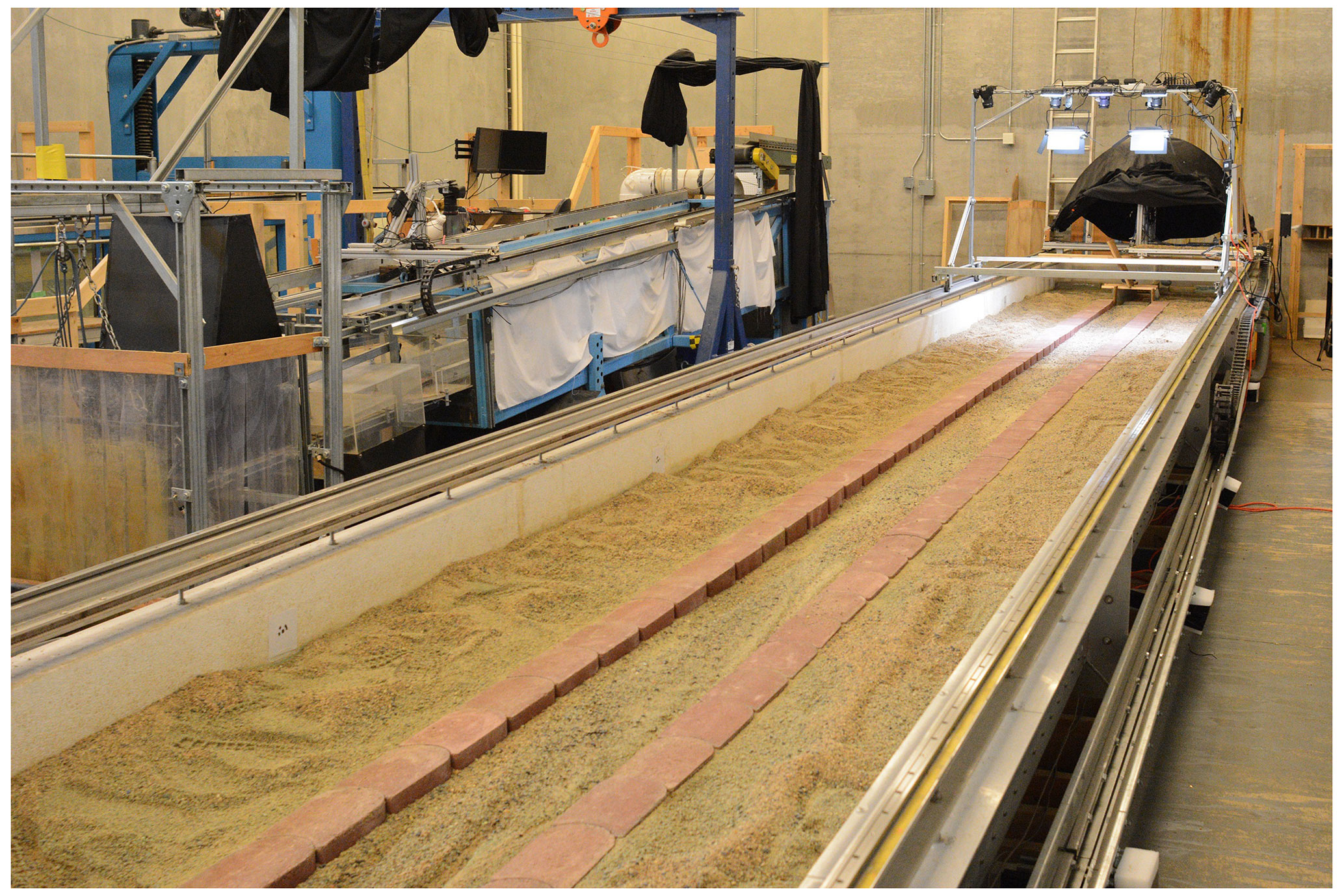
Figure 1 Adjustable-Boundary Experimental System (A-BES) at the University of British Columbia, featuring camera rig (top right) and bank control system at a width of 30 cm.

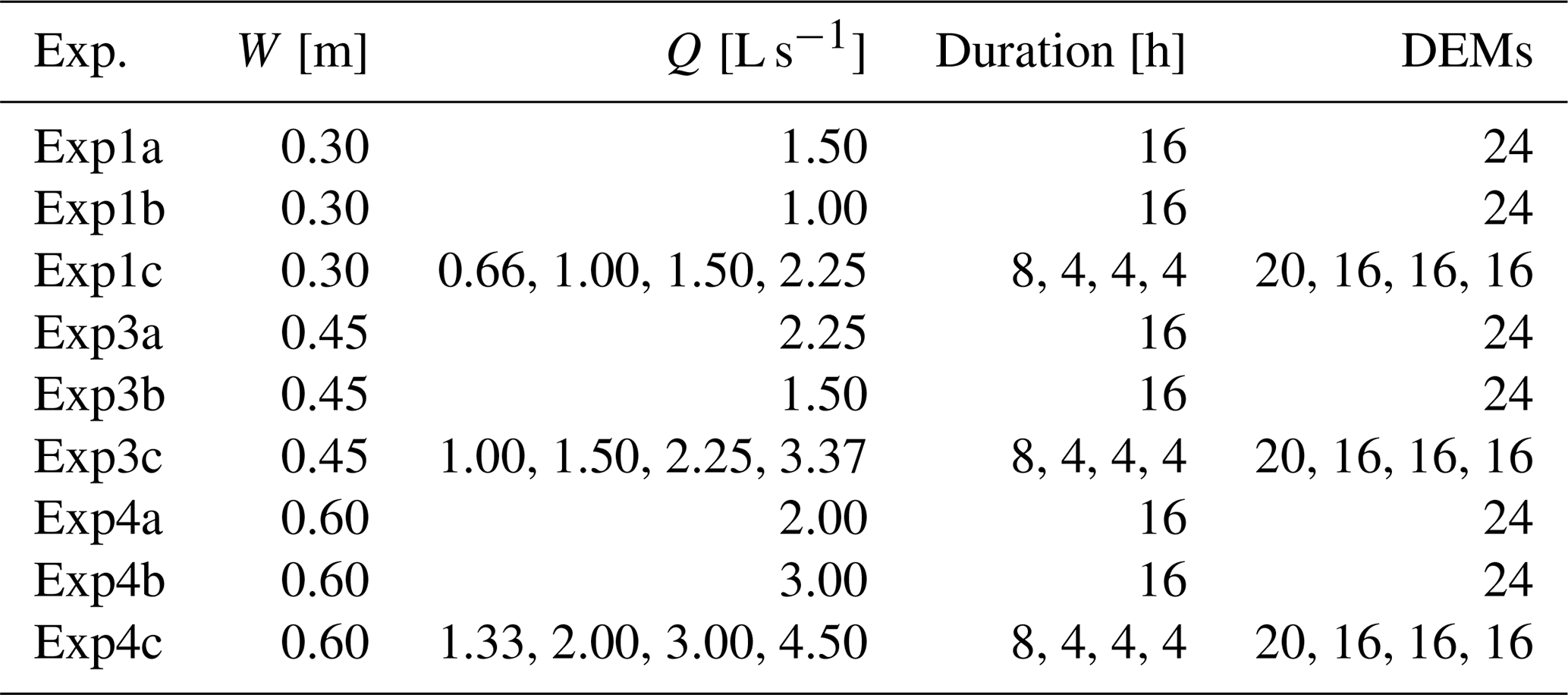
The experiments utilised interlocking landscaping bricks to constrict the channel to various widths W between approximately 0.30 and 0.60 m. In addition to the various channel widths, four different unit discharges ($q=Q/W$) were used across the experiments (i.e. discharge was scaled by width) that increased by a factor of 1.5 (Table 1). Two constant-discharge runs used the middle two discharges, and one multi-discharge run consisted of the four discharge phases in increasing order. A full list of experiments is provided in Table 2.

Table 1 Summary of unit discharges q ($Q/W$) used in each phase (P) of experimental runs a–c.

Table 2 Summary of experiments conducted in the A-BES. The DEM count excludes screeded bed. Experiment 1 is published in Adams and Zampiron (2020).

At the beginning of each experiment the bulk mixture was mixed by hand to minimise lateral and downstream sorting, and then the in-channel area was screeded to the height of weirs at the upstream and downstream end using a tool that rolled along the brick surface. The flow was run at a low rate with little to no movement of sediment until the bed was fully saturated, and it was then rapidly increased to the target flow.

Three different types of data were collected throughout each experiment; surface photos, stream gauge measurements, and sediment output. A rolling camera rig positioned atop the A-BES consisted of five Canon EOS Rebel T6i DSLRs with EF-S 18–55 mm lenses (set at 30 mm) positioned at varying oblique angles in the cross-stream direction to maximise coverage of the bed, as well as five LED lights. Photos were taken in RAW format at 0.2 m downstream intervals, providing a stereographic overlap of over two-thirds. A total of 10 water stage gauges comprised of a measuring tape on flat boards were located along the inner edge of the bricks every 1 m. To minimise edge effects, gauges were not placed within 0.60 m of either the inlet or the outlet. The gauges were read at an almost horizontal angle, which, in conjunction with the dyed blue water, minimised systematic bias towards higher readings due to surface tension effects.

The data collection procedure was designed to maximise measurement accuracy as much as reasonably possible. Given that stream gauge data would later be paired with topographic data, the timing of gauge readings needed to closely coincide with surface photography. Every time photos were taken the bed was drained, as the surface water would distort the photos. These constraints necessitated a procedure in which manual stream gauge readings (to the nearest 1 mm) were taken 30–40 s before the bed was rapidly drained, which is around the minimum time it would take to obtain the readings. The bed was then photographed and gradually re-saturated before resuming the experiment, which took approximately 10 min.

Each discharge phase was divided into a series of segments between which the data were collected. The procedure occurred in 5, 10, 15, 30, 60, and 120 min segments with four repeats of each (i.e. 4×5 min, 4×10 min, and so on), which was designed to reflect the relatively rapid rate of morphologic change at the beginning of each phase. For example, in wider channels, alternate bars developed within an hour, and there was relatively little morphologic change in the following hours (Adams and Zampiron, 2020; Adams, 2021).

Throughout the experiments, sediment falling over the downstream weir was collected in a mesh bucket, drained of excess water, weighed damp to the nearest 0.2 kg, placed on the conveyor belt at the upstream end, and gradually recirculated at the same rate it was output, as opposed to a “slug” (i.e. all at once) injection. Based on a range of samples collected across the experiments, we determined the weight proportion of water to be approximately 5.8 % and applied this correction factor to obtain approximate dry weights. There was no initial feed of sediment, although this no-feed period was only 5 min. The experiments are best described as pseudo-recirculating as sediment was measured and recirculated at the end of the 5 and 10 min segments and, for longer segments (i.e. 30, 60, 120 min), every 15 min.

2.1 Data processing

Using the images, point clouds were produced using structure-from-motion photogrammetry in Agisoft MetaShape Professional 1.6.2 at the highest resolution, yielding an average point spacing of around 0.25 mm. A total of 12 spatially referenced control points and additional unreferenced ones were distributed throughout the A-BES, which placed photogrammetric reconstructions within a local coordinate system and aided in the photo-alignment process. Using inverse distance weighting, the point clouds were converted to digital elevation models (DEMs) at 1 mm horizontal resolution.

Despite the use of control points, the DEMs contained a slight arch effect in the downstream direction whereby the middle of the model was bowed upwards, which was an artefact of the photogrammetric reconstruction (see doming: James and Robson, 2014). This effect was first quantified by applying a quadratic function (on average: p<0.001, r²=0.999, RMSE =0.0017 mm) along the length of the bricks, which represent an approximately linear reference elevation (brick elevations vary randomly by ±2 mm). The arch was then removed by determining correction values along the length of the DEM using the residuals, which were then applied across the width of the model. The final least-squares linear fit along the brick surface was homoscedastic with an average root mean square error (RMSE) of 0.0018 mm (around the maximum height difference between adjacent bricks), indicating that the DEM was successfully corrected.

For each DEM, 10 wetted cross-sections were reconstructed using the water surface elevation data, which were then used to estimate reach-averaged hydraulics. For more detailed spatial analysis, the flow conditions of water depth and shear stress were reconstructed using a 2D numerical flow model (Nays2DH) to the final DEM of each discharge phase. The selection of the final DEM was arbitrary as any DEM over the steady-state portion of the experiment could have been selected. Nays2DH is a two-dimensional, depth-averaged, unsteady flow model that solves the Saint-Venant equations of free surface flow with finite differencing based on a general curvilinear coordinate system (further details can be found in Nelson et al., 2016). Notably, local shear stress is calculated using the bed friction coefficient and depth-averaged flow velocity components. Key input boundary conditions are the channel DEM, an initial estimate of reach-averaged Manning's n, cell resolution, and the water discharge. We selected an n value of 0.045 based on the channel conditions, a cell resolution equivalent to 5 mm, and a flow duration of 200 s, which was sufficient to establish convergence. After an initial model run, we back-calculated a spatially variable value using the flow resistance law presented by Ferguson (2007) that accounts for the influence of relative roughness,

$$\begin{array}{}\text{(1)}& (\mathrm{8}/f{)}^{\mathrm{1}/\mathrm{2}}={\displaystyle \frac{a_{\mathrm{1}}{a}_{\mathrm{2}}(d/k)}{(a_{\mathrm{1}}^{\mathrm{2}}+a_{\mathrm{2}}^{\mathrm{2}}(d/k{)}^{\mathrm{5}/\mathrm{3}}{)}^{\mathrm{1}/\mathrm{2}}}},\end{array}$$

where f is the Darcy–Weisbach friction factor, a₁ and a₂ are empirically derived coefficients, d is local flow depth, and the representative roughness length k=D₈₄. The spatially variable roughness value was used as an input to run the solver again.

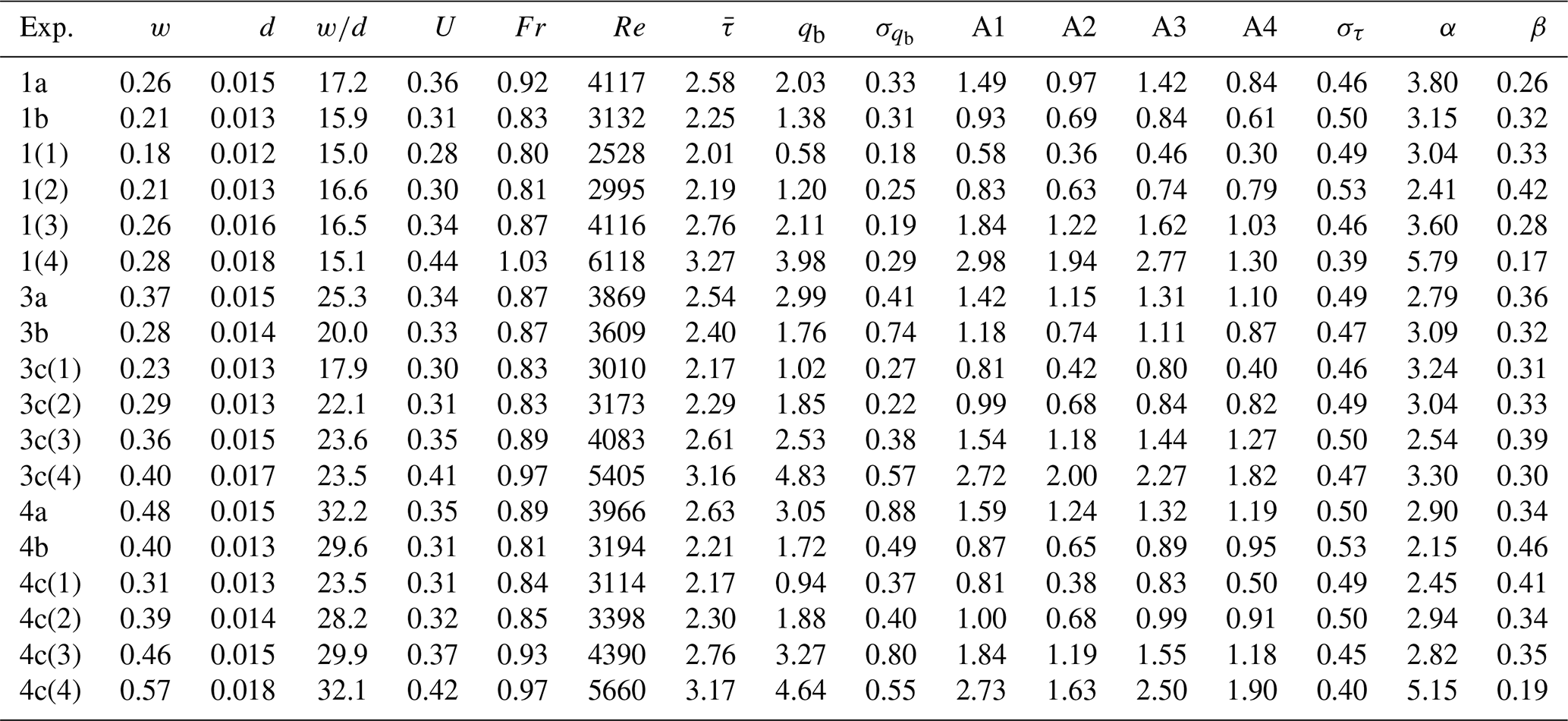
To minimise rounding errors associated with the relatively shallow depths in our experiments, the DEM size and discharge were adjusted to the prototype scale (i.e. using a length scale ratio of 25). The estimated water depths, shear stresses, and velocities from Nays2DH were then back-transformed to the model scale (Table 3). We removed cells with relatively shallow flows defined arbitrarily as depths less than 2D₈₄ (6.4 mm) as they contributed a large peak in the frequency distribution of flow depths and likely account for a small proportion of bedload activity. Across the flow models, grid cells with flows less than this threshold accounted for 20 %–63 % of the channel area where d>0 but only 1 %–21 % of the total cross-sectional flow area (mean 11 %). This is consistent with visual observations of dispersive and stagnant flow at the channel margins. We defined areas of the bed with flows above the 2D₈₄ threshold as “wetted”. The mean-normalised (i.e. local value divided by reach average) frequency distributions of flow depths and shear stresses were fitted with gamma and Gaussian distributions (coefficients in Table 3), for which the goodness of fit was assessed using both Kolmogorov–Smirnov and Anderson–Darling tests.

Table 3 Summary of reach-averaged hydraulics (from the 2D flow model) and sediment transport (from measurements). Parameters are as follows. w: wetted width [m], d: flow depth [m], U: velocity [m s⁻¹], Fr: Froude number, Re: Reynolds number ($Ud/v$, where v is the kinematic viscosity), $\overline{\mathit{\tau }}$: mean shear stress [Pa], q_b: unit bedload transport [kg m⁻¹ min⁻¹]. ${\mathit{\sigma }}_{q_{\mathrm{b}}}$ is the standard deviation of unit bedload transport, σ_τ is the standard deviation of shear stress, and α and β parameters describe the fitted gamma distribution of shear stress. The parameters A1, A2, B1, and B2 refer to the four approaches outlined in Table 4.

The results of the flow model were quantitatively validated by comparing measured reach-averaged hydraulic depths ($h=A_{\mathrm{c}}/w$, where A_c is flow cross-sectional area and w is wetted width) to modelled ones (Fig. 2). Most estimates fell within 10 %–15 % of the line of equality, although the flow model estimated a narrower range (approximately 12–18 mm) of mean hydraulic depths across the experiments compared to the stream gauge measurements (11–21 mm). Stream gauges are easily biased towards deep or shallow flows due to there being only 10 fixed points, thus explaining the wider range of the estimates. The stream gauges only serve as an approximation to validate the flow model. Based on the measurement precision of the stream gauge readings (1 mm), random errors of 6 %–11 % could be expected for mean hydraulic depths.

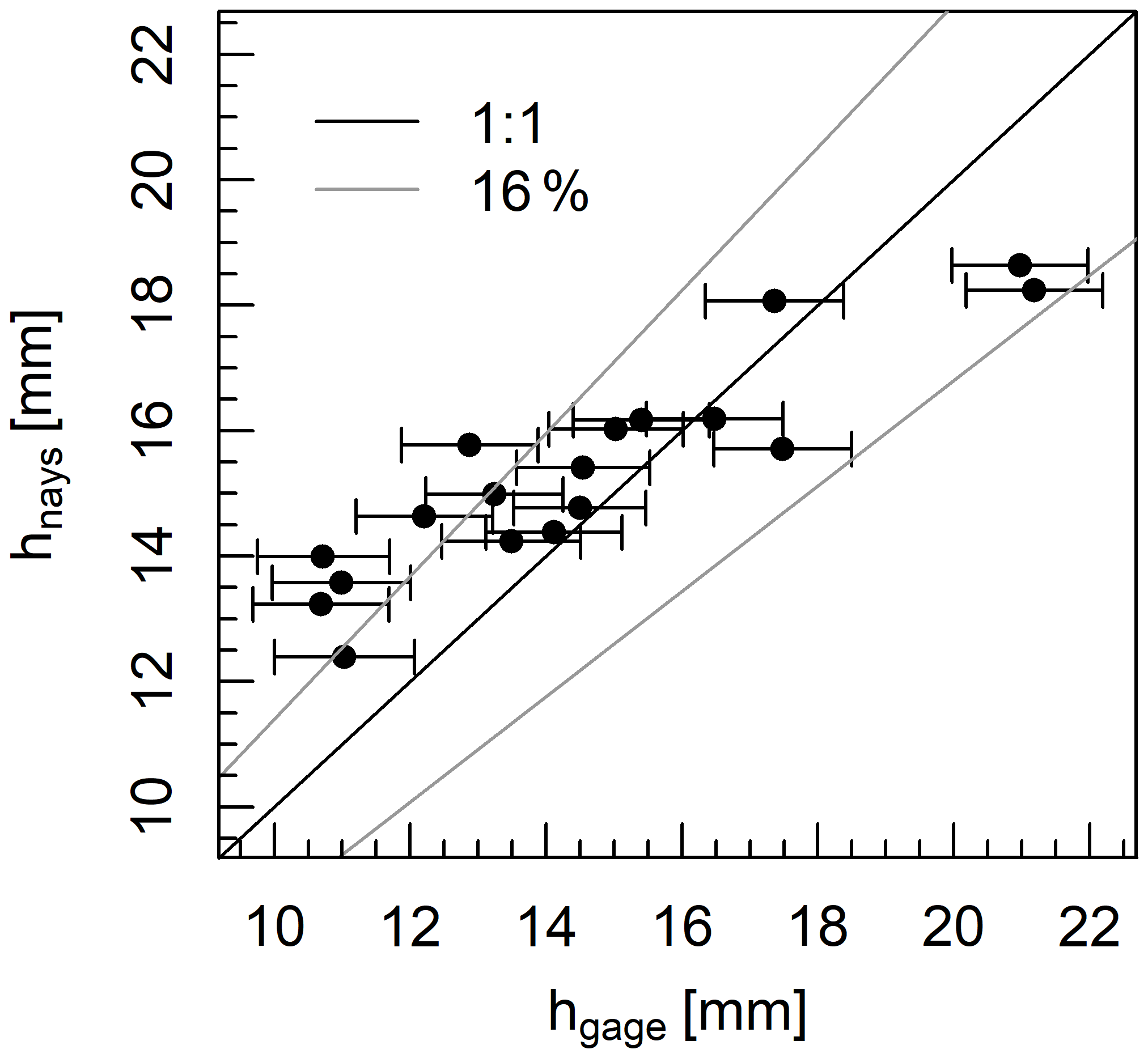
Figure 2 Measured versus modelled mean hydraulic depth h (i.e. reach-averaged) at the end of each experimental phase, featuring 16 % bounds. Error bars are based on the measurement precision of the stream gauges.

2.2 Determining a representative sediment transport rate

The channels were formed under constant-discharge conditions for 4–16 h, beginning from either a screeded bed or a morphology developed at a lower discharge. Each experimental phase comprised an initial adjustment period during which morphology, hydraulics, and sediment transport were nonstationary. This adjustment period, which varied from minutes to an hour, was followed by a steady-state period during which these characteristics fluctuated around a mean value (see Adams, 2020, and Adams and Zampiron, 2020). Under recirculating conditions, the stationarity of bedload transport represents a condition in which there is no net aggradation or degradation over time. In Fig. 3 we present two typical examples of sediment transport fluctuations under constant conditions for 16 h. In both examples, there is a brief adjustment period with less sediment transport, followed by fluctuations around a mean value. These fluctuations were explained by processes such as bar reshaping and sediment waves (e.g. Dhont and Ancey, 2018), which are outside the scope of this study.

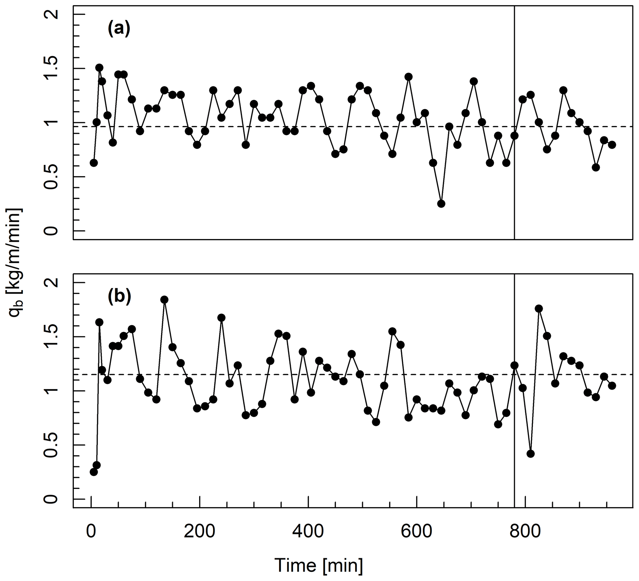
Figure 3 Width-averaged bedload transport over time in two experiments with different widths but similar reach-averaged shear stress: (a) experiment 1b (W=0.30 m, $\overline{\mathit{\tau }}=\mathrm{2.34}$ Pa) and (b) experiment 4b (W=0.60 m, $\overline{\mathit{\tau }}=\mathrm{2.28}$ Pa). The beginning of the time window over which bedload transport is averaged is indicated by the solid vertical line, and mean transport over this period is indicated by a horizontal dashed line.

We determined a representative sediment transport rate for each experimental phase by averaging output over the final 3 h period (Table 3), thus removing the initial adjustment period. There was little difference between averaging over the final hour versus the final 3 h, with almost all average sediment output values being ±12.5 %. There were three instances in which these two averaging windows yielded values differing by 15 %–25 % due to high-magnitude fluctuations around an otherwise stationary bedload transport rate. In addition, we calculated the standard deviation of sediment output over the final 3 h period.

2.3 1D and 2D excess shear stress

We examined the correlation between the observed representative sediment transport rate and two formulations of excess shear stress based on the Meyer-Peter and Müller (1948) equation,

$$\begin{array}{}\text{(2)}& q_{\mathrm{b}}=k(\overline{\mathit{\tau }}-{\mathit{\tau }}_{\mathrm{c}}{)}^{\mathrm{1.6}},\end{array}$$

where q_b is width-averaged bedload transport, k accounts for flow resistance and the relative density of sediment, and the exponent 1.6 is based on Wong and Parker (2006). The value of k is highly variable across empirical datasets, whereas the exponent is relatively consistent (Gomez and Church, 1989). The critical shear stress value for the D₅₀ (τ_c50) is estimated by ${\mathit{\tau }}_{\mathrm{c}}^{*}g({\mathit{\rho }}_{\mathrm{s}}-\mathit{\rho })D$, where ${\mathit{\tau }}_{\mathrm{c}}^{*}$ is the dimensionless critical shear stress, g is gravity, ρ is the density of water, and ρ_s is the density of sediment

We aimed to investigate the concepts underlying 1D and 2D bedload transport equations rather than to refine them. Subsequently, we ignored the parameter k that typically varies across channels and simplified Eq. (2) to express the correlation between observed sediment transport and mean excess shear stress (raised to the exponent).

$$\begin{array}{}\text{(3)}& q_{\mathrm{b}}\propto {\left(\overline{\mathit{\tau }}-{\mathit{\tau }}_{\mathrm{c}\mathrm{50}}\right)}^{\mathrm{1.6}}\end{array}$$

This equation was modified to integrate across the distribution of local shear stresses,

$$\begin{array}{}\text{(4)}& q_{\mathrm{b}}\propto \int ({\mathit{\tau }}_{\left(x\right)}-{\mathit{\tau }}_{\mathrm{c}\mathrm{50}}{)}^{\mathrm{1.6}}\mathrm{d}x/A,\end{array}$$

where τ_(x) is local bed shear stress and A is the total bed area. Equations (3) and (4) are 1D and 2D approaches to correlating observed transport capacity with excess shear stress. We applied both equations using shear stress values calculated in two ways: (1) the depth–slope product (τ=ρgdS) based on numerically modelled flow depths and (2) numerically modelled shear stresses, thus yielding four different approaches (Table 4). Each of these approaches is summarised in Appendix A. We intentionally did not account for sinuosity or sidewall effects in the depth–slope product approach. In the case of the 1D depth–slope approach, depth was calculated using the mean depth and mean channel gradient, whereas in the 2D depth–slope we varied depth but the gradient remained constant. For each approach, we back-calculated the optimal value of ${\mathit{\tau }}_{\mathrm{c}}^{*}$ by systematically varying it and finding the strongest correlation (least-squares linear fit) between q_b and excess shear stress (i.e. $[\overline{\mathit{\tau }}-{\mathit{\tau }}_{\mathrm{c}\mathrm{50}}{]}^{\mathrm{1.6}}$ or $\mathrm{\Sigma }{\left[{\mathit{\tau }}_x-{\mathit{\tau }}_{\mathrm{c}\mathrm{50}}\right]}^{\mathrm{1.6}}/A$), indexed by root mean square error (RMSE), which is shown in Fig. 4. We report optimised values of ${\mathit{\tau }}_{\mathrm{c}}^{*}$ and least-squares goodness-of-fit statistics in Table 4 and also include values obtained using the exponent 1.5 in each equation.

Table 4 Optimised values of ${\mathit{\tau }}_{\mathrm{c}}^{*}$ and goodness-of-fit statistics for correlations between excess shear stress and observed bedload transport using four different approaches. Values obtaining using the exponent 1.5 are presented in parentheses, and $\overline{\mathit{\tau }}/{\mathit{\tau }}_{\mathrm{c}\mathrm{50}}$ represents the range of relative shear stress values across the experiments.

Figure 4 The correlation between q_b and excess shear stress (indexed by RMSE) with varying critical dimensionless shear stress for each approach. A back-calculated critical dimensionless value is indicated where RMSE is lowest (Table 4).

3 Results

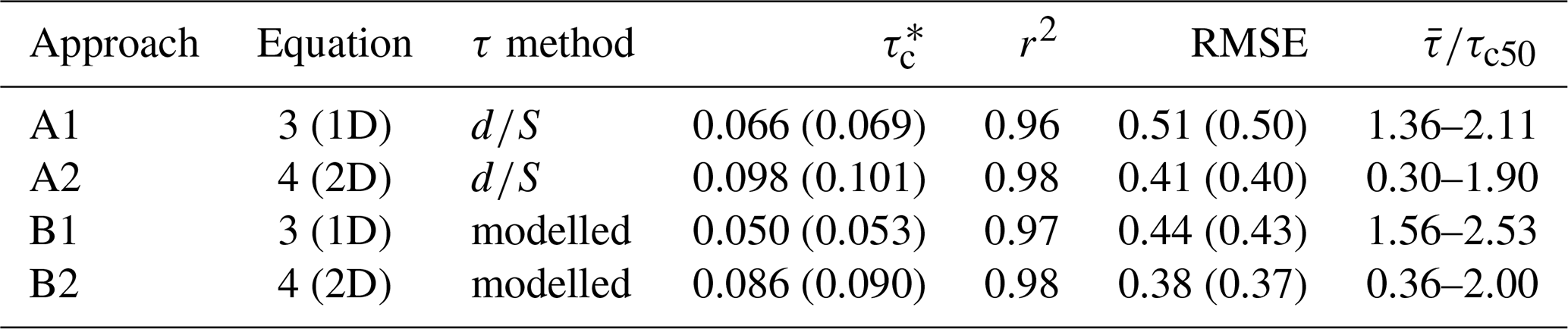
Under the imposed channel widths (0.30–0.60 m) and unit discharges (2.22–7.50 L m⁻¹ s⁻¹) all channels developed an alternate bar morphology with pools, bars, and riffles (see Fig. 5 for an example). Especially at low unit discharges, wetted areas (d>2D₈₄) on average occupied only a portion of the total available width: between 52 % and 95 %. When unit discharge was calculated using the wetted width, it was closely correlated with mean shear stress based on least-squares linear regression (Fig. 6a), indicating a coupled adjustment between active width and shear stress.

Figure 5 Channel area at the conclusion of experiment 3b (W=0.45 m, $\overline{\mathit{\tau }}=\mathrm{2.41}$ Pa) displaying the following characteristics (a–c): (a) elevation, (b) flow depth, and (c) shear stress from the flow model. Cells where d<2D₈₄ are not shown. A transect along the path of the highest bed shear stress is displayed as a black line.

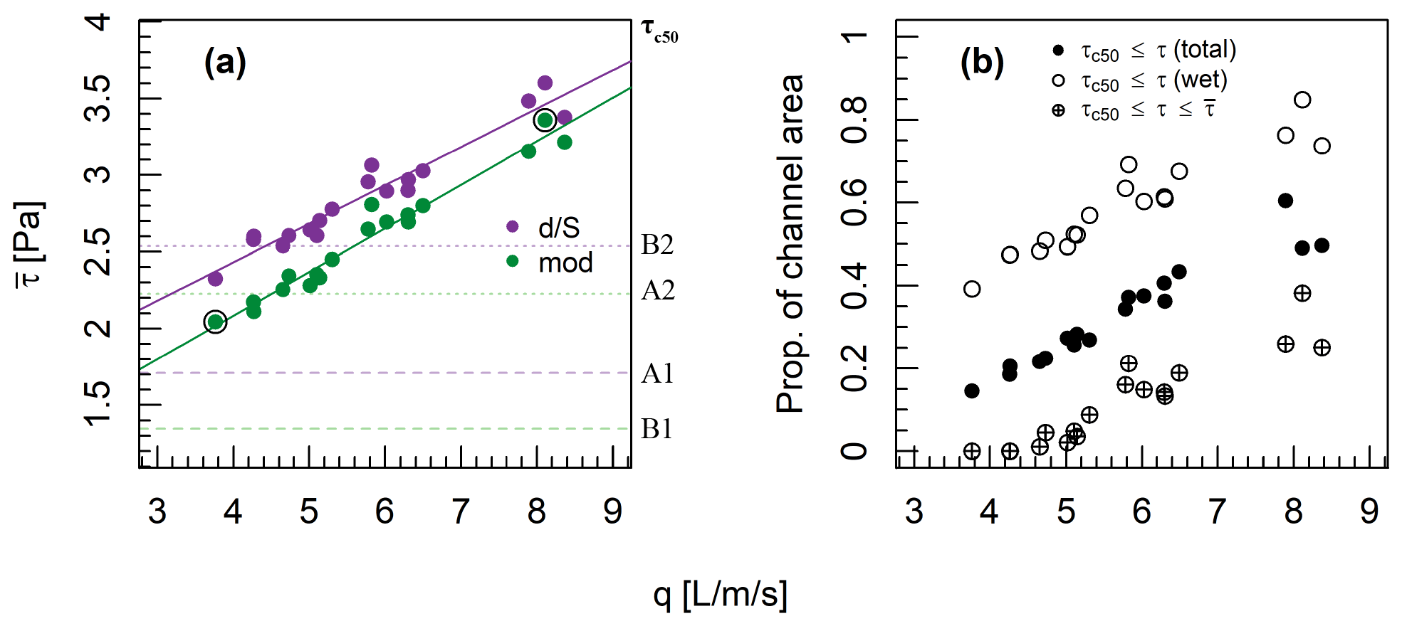
Figure 6 (a) Relationship between unit discharge q (calculated using wetted width) and mean shear stress $\overline{\mathit{\tau }}$ using depth–slope product (RMSE =0.097, r²=0.93, p<0.001) and modelled shear stresses (RMSE =0.073, r²=0.96, p<0.001). Horizontal lines indicate fitted values of τ_c50, and circled points indicate channels with the highest and lowest shear stress used in Fig. 7b. (b) Relationship between unit discharge and the proportion of the wetted channel area (d>2D₈₄) where τ>τ_c50 using modelled shear stresses (i.e. approach B2), as well as the proportion of channel area where ${\mathit{\tau }}_{\mathrm{c}\mathrm{50}}<\mathit{\tau }\le \overline{\mathit{\tau }}$.

The depth–slope method of calculating mean shear stress estimated higher values compared to the numerical model (7 %–23 %) and also higher values of critical dimensionless shear stress in the corresponding transport functions (${\mathit{\tau }}_{\mathrm{c}}^{*}=\mathrm{0.066}$ and 0.050, respectively; Table 4). Both methods yielded similar estimates of excess shear stress ($\overline{\mathit{\tau }}/{\mathit{\tau }}_{\mathrm{c}\mathrm{50}}=\mathrm{1.36}$–2.11 and 1.56–2.53, respectively). The strong correlation between the two estimates of shear stress supports the assumption that at the reach scale $\overline{\mathit{\tau }}\approx \mathit{\rho }gdS$.

Estimated values of ${\mathit{\tau }}_{\mathrm{c}}^{*}$ using the 2D approaches were consistently higher than the values obtained using the 1D approaches, but they were slightly less sensitive to how shear stress was calculated (${\mathit{\tau }}_{\mathrm{c}}^{*}\approx \mathrm{0.095}$ for both methods). Based on the 2D approach, the proportion of the wetted bed area experiencing excess shear stress was linearly related to unit discharge and ranged between 37 % and 84 % (Fig. 6b). In several experiments 2D estimates of τ_c50 were higher than $\overline{\mathit{\tau }}$.

Local shear stresses at or below the mean were estimated to exceed τ_c50 only at unit discharges exceeding approximately 5 L m⁻¹ s⁻¹ (Fig. 6). This range of shear stresses (i.e. ${\mathit{\tau }}_{\mathrm{c}\mathrm{50}}<\mathit{\tau }<\overline{\mathit{\tau }}$) accounted for up to 37 % of the total bed area at the highest flows. These results indicate considerable shear stress concentration and the relative insignificance of moderate shear stresses in bedload transport. We further visualise shear stress distributions and estimated critical values using examples in Fig. 7b.

Figure 7 (a) Cumulative frequency distributions of mean-normalised modelled flow depth and shear stress at the end of each experimental phase, in which the upper end of the kernel density distribution has been truncated to approximately the 99th percentile to remove outliers. Note the absence of shallow depths (d<2D₈₄). The average gamma distribution fit for the normalised shear stress distribution is included ($\mathit{\alpha }=\mathrm{3.30},\mathit{\beta }=\mathrm{0.30}$), as is the average Gaussian fitted distribution (σ=0.47). (b) Cumulative frequency distribution of non-normalised modelled shear stresses in experimental phases with the highest (Exp1c(4)) and lowest (Exp1c(1)) mean shear stress (circled points in Fig. 6). Estimates of τ_c50 using 1D and 2D approaches (B1 and B2, respectively) are indicated by dashed lines, and the horizontal line is the median shear stress, which closely corresponds to the mean.

Frequency distributions of mean-normalised flow depth and shear stress (over each 5×5 mm grid cell) followed both Gaussian and gamma distributions (Fig. 7a), confirmed by both Kolmogorov–Smirnov and Anderson-Darling tests (p<0.1). These distributions were qualitatively similar based on their cumulative distributions following the removal of shallow depths, which contributed a second mode of flow depths corresponding to dispersive flow or stagnant water at the channel margins. In the case of the shear stress distributions, the shape parameter α was linearly related to unit discharge based on least-squares regression (RMSE =0.69, r²=0.39, p<0.01), and the scale parameter β was negatively correlated (RMSE =0.58, r²=0.32, p<0.01). The parameters of the gamma distribution indicate that with increasing unit discharge the distribution of shear stress became more concentrated and less positively skewed.

Despite following similar frequency distributions, modelled local flow depth and shear stress were not strongly coupled spatially (Fig. 8). These two parameters were roughly correlated but with considerable scatter, whereby for a given grid cell mean-normalised shear stress was commonly more than a factor of 2 greater or less than normalised flow depth (i.e. high shear stress and deep flows are close but not at exactly the same locations). The spatial decoupling of flow depth and shear stress is also evident in Fig. 5, especially where areas of high shear stress are estimated to occur immediately downstream of pools where flow is deepest.

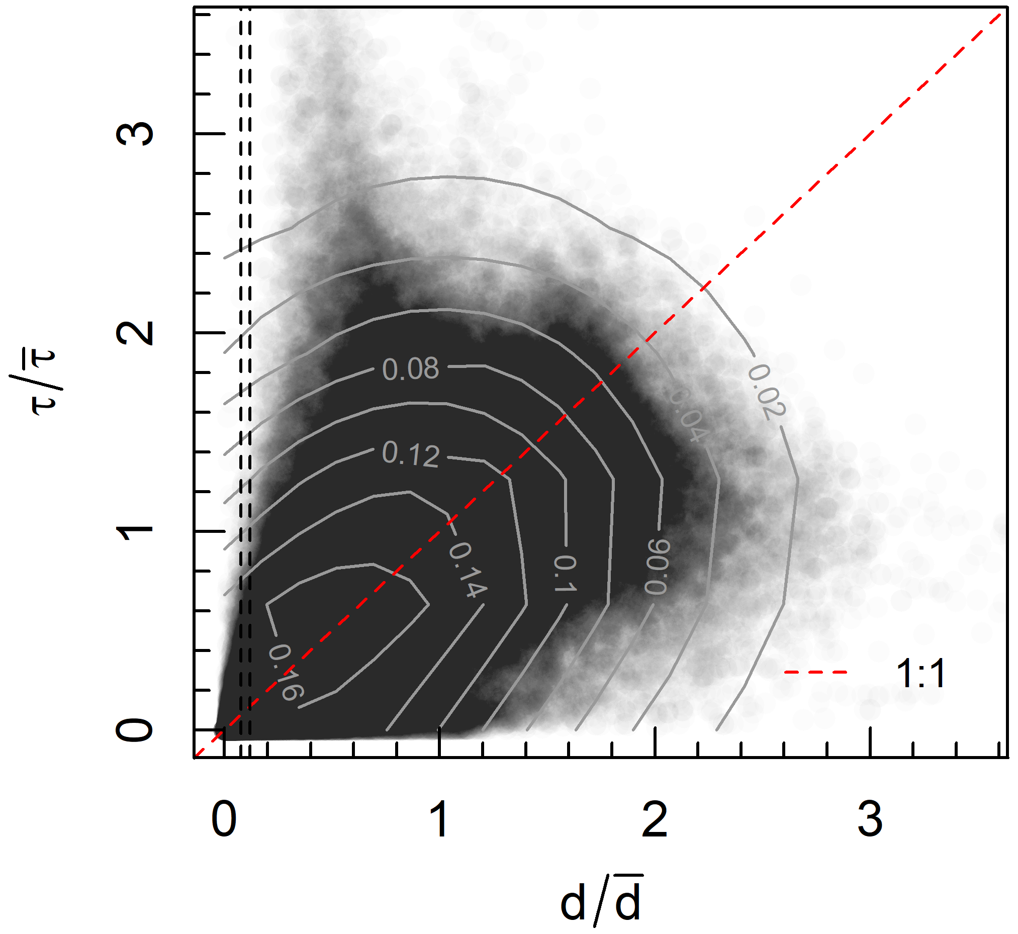
Figure 8 Relationship between local mean-normalised flow depth and shear stress across all experiments, produced by randomly sampling 10 % of cells from each flow model. Contour lines represent 2D kernel density estimation, and vertical dashed lines indicate the range of flow depths used to threshold the flow model.

We present the correlation between bedload transport and the four different representations of excess shear stress in Fig. 9. These represent combinations of two different methods of calculating bed shear stress – the depth–slope product and numerical modelling – against 1D and 2D representations of excess shear stress (Table 4). All four methods yielded similar correlations between excess shear stress and observed bedload transport, as indicated by RMSE values between 0.38 and 0.51; these end values correspond to the 2D modelled shear stress (B2) and 1D depth–slope product approach (A1), respectively. Changing the exponent from 1.6 to 1.5 in Eqs. (3) and (4) had almost no effect on the estimated values of ${\mathit{\tau }}_{\mathrm{c}}^{*}$ or the prediction errors. Altering the representative grain size from D₅₀ to D₈₄ had no effect on the correlation between q_b and excess shear stress (i.e. identical RMSE), and it merely reduced the back-calculated estimates of ${\mathit{\tau }}_{\mathrm{c}}^{*}$.

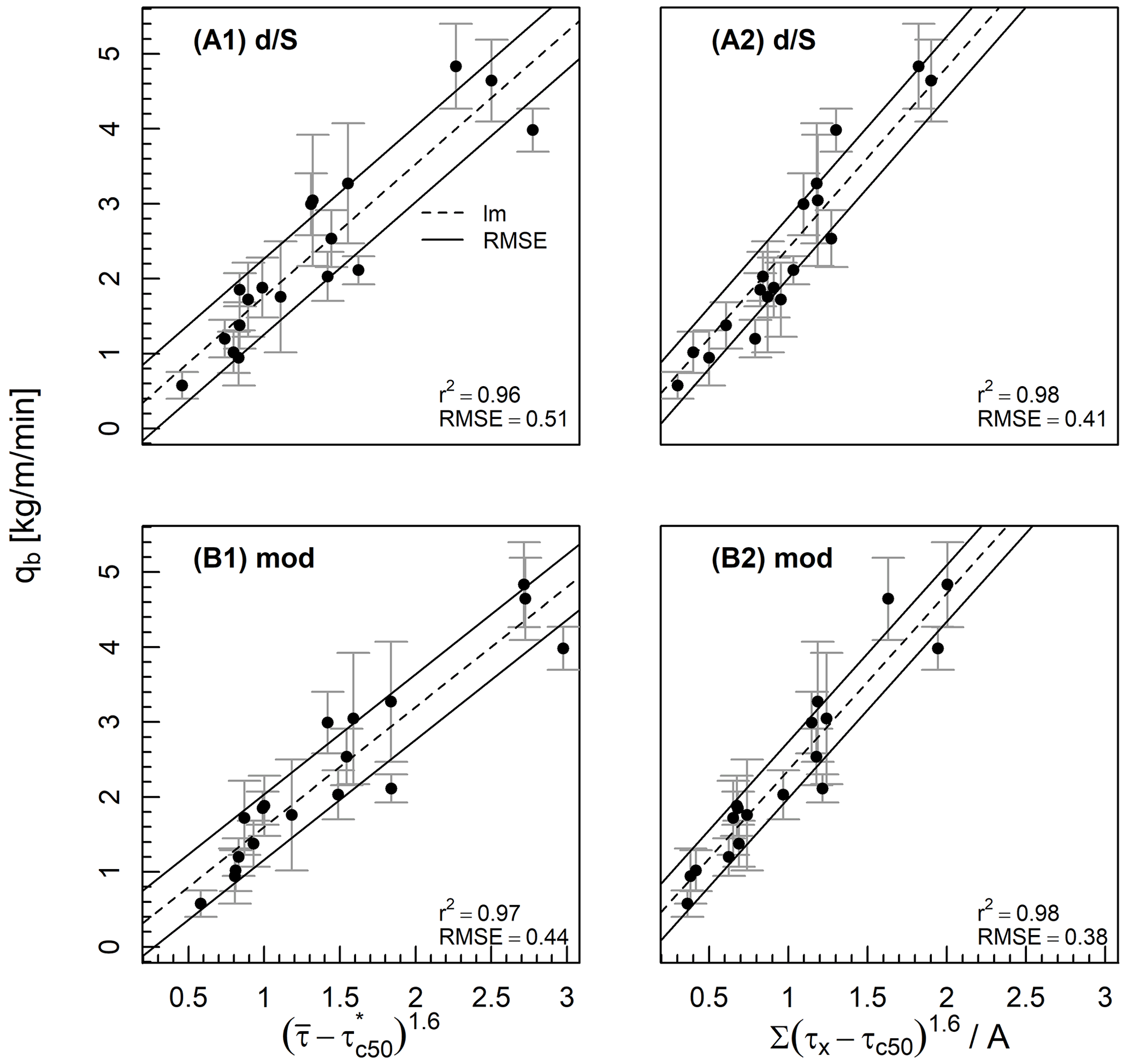
Figure 9 Correlation between excess shear stress and observed bedload transport (averaged over the final 3 h of each experiment) using the four approaches outlined in Table 4. The dashed black line is the least-squares best fit, solid black lines indicate ±1 RMSE, and whiskers indicate ±1 standard deviation over the final 3 h of sediment output measurements.

4 Discussion

These experiments had several advantages over traditional field and flume datasets in modelling and recording channel processes. Although the experiments did not model lateral adjustment, the smaller scale ratio (1:25) allowed for morphology and processes at a larger scale compared to most flumes with width–depth ratios between approximately 15 and 40. The bulk mixture comprised a wide range of grain sizes (0.5–8.0 mm) that have been demonstrated to modulate channel adjustment, especially under conditions in which the larger-than-average grain size is only partially mobile (MacKenzie and Eaton, 2017; MacKenzie et al., 2018; Booker and Eaton, 2020; Adams, 2021). We measured total bedload volumes and adjustments to bed topography during flood stages, which is not possible in the field or in many recirculating experiments. The applied flows were longer and more constant than floods typically observed in nature (4–16 h experimental time or 20–80 h in the field prototype), which allowed the experiments to reach an idealised steady state whereby morphology, hydraulics, and bedload fluctuated around a mean condition (Fig. 3). These characteristics make the experimental dataset appropriate for investigating the effectiveness of bedload transport equations in laterally constrained gravel-bed rivers under high relative shear stress conditions.

We evaluated four different bedload transport functions based on the correlation between excess shear stress and observed volumes of bedload transport, averaged over the final 3 h of each experimental phase. We first focus our discussion on three of these approaches in increasing order of sophistication (A1, B1, then B2) and then explain their relative effectiveness. Finally, we discuss the conceptual differences between 1D and 2D bedload transport functions.

4.1 Comparison between prediction errors

Most bedload transport functions index the applied excess shear stress using the mean depth–slope product as these data are relatively easy to collect in field contexts (Gomez and Church, 1989; Barry et al., 2004; Recking, 2013b). This approach relies on the assumption that local variations in channel gradient and flow depth cancel out such that mean flow depth is proportional to mean shear stress (Nicholas, 2000; Ferguson, 2003). We did indeed observe this condition whereby mean-normalised flow depth and shear stress followed similar frequency distributions (Fig. 7a), despite being spatially decoupled (Fig. 8). The approach A1 (1D depth–slope product) in our analysis was the most simplistic and, in addition, did not account for sinuosity (note the slight sinuosity in Fig. 5 that reduced the mean channel gradient), flow resistance, or energy losses to the channel banks. The strength of the correlation between excess shear stress and bedload transport (RMSE =0.51) provides an approximate reference point for other approaches.

In recent decades, technological advancements in remote sensing and hydraulic modelling have allowed researchers to directly model bed shear stress, thus providing a potentially more accurate estimate. This advancement is utilised in the B1 approach (1D modelled shear stress), which accounted for the effect of sinuosity, flow resistance, and energy losses to the channel banks. Accounting for these additional factors may explain the 13 % reduction in RMSE (0.44) compared to approach A1. Further advancements have led to the proliferation of 2D hydraulic models and some 2D bedload transport equations, which aim to account for the proportion of the bed participating in transport and the spatial variation in shear stress (Monsalve et al., 2020). The B2 approach (2D modelled shear stress) that integrates across the frequency distribution of shear stresses did not significantly improve upon approach A1, with a similar RMSE (0.38) as approach B1.

Numerical modelling of shear stress and accounting for its frequency distribution led to similarly strong correlations between bedload transport and excess shear stress compared to the mean depth–slope product method. The ability of the mean shear stress to effectively capture variation in bedload transport is consistent with empirical evidence. In a reanalysis of data from Oak Creek, OR, Monsalve et al. (2020) compared the Parker and Klingeman (1982) equation to a modified 2D version and found that accounting for the distribution of shear stresses reduced prediction error by only 13 %. Their study modelled a range of flows to the same bathymetry, and we obtained a similar result when the bed was allowed to fully adjust to the imposed flow. Using numerical and analytical models, several studies have predicted that variance in shear stress may enhance bedload transport but that this effect rapidly diminishes when $\overline{\mathit{\tau }}\gg {\mathit{\tau }}_{\mathrm{c}}$ (Ferguson, 2003; Francalanci et al., 2012; Recking, 2013a). The most probable reason for this sensitivity is the nonlinearity of the bedload transport law, which means that around $\overline{\mathit{\tau }}\approx {\mathit{\tau }}_{\mathrm{c}}$ small increases in τ produce relatively large increases in bedload transport. The similar effectiveness of 1D and 2D functions herein provides empirical evidence that bedload transport is less sensitive to the shape of the shear stress distribution under high relative shear stress conditions.

4.2 Comparison between 1D and 2D approaches

The four approaches demonstrated key differences based on how shear stress was calculated (depth–slope product vs. numerical modelling) and more importantly the formulation (1D vs. 2D). Both estimates of mean shear stress were linearly related to unit discharge, but those based on the depth–slope product were 7 %–23 % higher (Fig. 6), which is consistent with findings by Monsalve et al. (2020). These differences in estimated shear stress led to approximately commensurate differences in the estimated 1D values of ${\mathit{\tau }}_{\mathrm{c}}^{*}$ (32 % higher). Both 1D estimates of ${\mathit{\tau }}_{\mathrm{c}}^{*}$ were relatively high for gravel-bed rivers but were within the range of reported estimates from both field and laboratory channels (Buffington and Montgomery, 1997).

Despite having similar prediction errors, the 1D and 2D functions provided considerably different estimates of critical dimensionless shear stress. Using the 2D approach, estimates of ${\mathit{\tau }}_{\mathrm{c}}^{*}$ were 48 % and 72 % higher than the 1D depth–slope and modelled shear stress methods, respectively. In several channels, the estimated critical shear stress was greater than the mean shear stress, but bedload transport was observed and well predicted by the model (Fig. 6), which in the case of a threshold-based 1D equation would correspond to zero estimated transport. This is a distinct advantage of 2D equations at low flows, as they can account for flows wherein excess shear stress occupies only a fraction of the bed (Monsalve et al., 2020).

The differences between estimates of ${\mathit{\tau }}_{\mathrm{c}}^{*}$ arise from differences in how the equations conceptualise excess shear stress. In a 1D equation, when bedload transport data are available, τ_c may be back-calculated from the mean shear stress, as is done herein. The value of ${\mathit{\tau }}_{\mathrm{c}}^{*}$ is adjusted until excess shear stress explains the observed bedload transport, assuming that $\overline{\mathit{\tau }}$ is responsible for all entrainment. In contrast, the 2D equation does not assume that the mean shear stress participates in bedload entrainment. Based on the 2D approach, we estimated that the mean shear stress did not exceed the estimated critical value for the D₅₀ until a certain discharge threshold (5 L m⁻¹ s⁻¹), and even under the highest flows these areas (i.e. ${\mathit{\tau }}_{\mathrm{c}\mathrm{50}}<\mathit{\tau }<\overline{\mathit{\tau }}$) characterised a maximum of 37 % of the wetted area. We did not validate these values as we did not anticipate the need for observation, although the estimates appear reasonable compared to our visual observations of the experiments. This result suggests that the mean shear stress is far less significant for bedload transport compared to the larger-than-average stresses, which is intuitive, especially given that these are the first stresses to entrain bed material as the flow is increased.

By conceptualising transport as a function of mean shear stress, 1D equations may inflate the importance of relatively moderate shear stresses and deflate values of ${\mathit{\tau }}_{\mathrm{c}}^{*}$. This insight is based on back-calculated values rather than measurements of incipient motion, although it is important to note that studies measuring incipient motion have also been based on the mean shear stress, and therefore this 1D paradigm is subsumed within the results (Gilbert, 1914; Kramer, 1935; Neill and Yalin, 1969; Wilcock, 1988). We also relied on spatio-temporally integrated rather than instantaneous local shear stresses that promote entrainment (e.g. Nelson et al., 1995). Nevertheless, the higher estimates of critical dimensionless shear stress using the 2D approach, evaluated by considering the relative importance of shear stresses across the frequency distribution, may have a stronger conceptual basis. More broadly, the results highlight that as long as τ_c is back-calculated, its value will be highly dependent on how shear stress is estimated and whether its distribution is treated one- or two-dimensionally.

The results may have implications for non-threshold approaches to predicting bedload transport in natural gravel-bed rivers (Parker et al., 1982; Parker, 1990; Wilcock and Crowe, 2003; Recking, 2013a). These approaches recognise that usage of a single critical shear stress is ineffective at low flows and is always an approximation, especially in the case of partial transport conditions in which not all grain sizes (or even grains of a given size) are equally mobile (Wilcock and McArdell, 1993). The effectiveness of threshold-based approaches under high excess shear stresses suggests that in channels with fully developed morphology and a wide range of grain sizes, non-threshold-based approaches may not render an improvement. Also, the results challenge recent critiques of bedload transport predictions based on mean shear stress, particularly the depth–slope assumption (Yager et al., 2018). Although there is a poor mechanistic link between shear stress and bedload transport (e.g. Nelson et al., 1995), this approximation may be unreasonably effective when applied at a sufficiently large spatio-temporal scale or excess shear stress.

Further work is required to investigate differences in 1D and 2D estimates of ${\mathit{\tau }}_{\mathrm{c}}^{*}$ under lower excess shear stress conditions. If broadly applicable, the effectiveness of highly reductionist bedload transport functions based only on median grain size and mean shear stress would present a convenient assumption for researchers and practitioners interested in channel-forming flows. More research is required to substantiate this approach under supply-limited conditions and realistic hydrographs that enable both upward and downward adjustments with inherited channel conditions. Given that our experiments do not allow for significant lateral adjustment and meandering, the results are most applicable to channels confined by bedrock or with cohesive or highly vegetated banks. Fully alluvial channels comprise additional feedbacks that are worthy of investigation, and the extent to which these affect reach-averaged bedload transport remains poorly understood.

5 Conclusions

We investigated the performance of 1D and 2D bedload transport functions under high relative shear stress conditions in a Froude-scaled physical model. The analysis highlights the effectiveness of highly reductionist bedload transport functions based only on median grain size and mean shear stress calculated using the depth–slope product. Numerically modelling shear stress to account for flow resistance and energy losses from the channel planform and banks did not substantially reduce prediction error, nor did accounting for the relative importance of shear stresses across the frequency distribution. The results suggest that bedload transport may collapse to a more simple function (i.e. with average shear stress and grain size) under high excess shear stress conditions. Given that the channels herein have limited lateral mobility, our conclusions are most applicable to channels where lateral adjustment is suppressed. Further work is required to examine the effect of planform adjustments (widening, meandering), for which small-scale laboratory experiments serve as an effective research tool. The 1D and 2D approaches provided substantially different estimates of critical dimensionless shear stress, reflecting differences in how these approaches conceptualise excess shear stress. Estimates of ${\mathit{\tau }}_{\mathrm{c}}^{*}$ from 2D functions may have a stronger conceptual basis, as they are derived by considering the relative importance of shear stresses across the frequency distribution and do not assume that the mean shear stress is sufficient to mobilise the median grain size.

Appendix A: Four bedload transport equations

A1 Approach A1: mean shear stress assuming depth–slope product

$$\begin{array}{}\text{(A1)}& q_{\mathrm{b}}\propto (\overline{\mathit{\tau }}-{\mathit{\tau }}_{\mathrm{c}\mathrm{50}}{)}^{\mathrm{1.6}}\end{array}$$

Here, q_b is unit bedload transport, $\overline{\mathit{\tau }}$ is estimated with ρgdS (where g is gravity, d is mean flow depth from a 2D flow model, and S is the channel gradient), and τ_c50 is estimated by ${\mathit{\tau }}_{\mathrm{c}}^{*}g({\mathit{\rho }}_{\mathrm{s}}-\mathit{\rho })D$, where ${\mathit{\tau }}_{\mathrm{c}}^{*}$ is the dimensionless critical shear stress chosen using the best fit (Table 4), ρ is the density of water, and ρ_s is the density of sediment.

A2 Approach A2: distribution of shear stresses assuming depth–slope product

$$\begin{array}{}\text{(A2)}& q_{\mathrm{b}}\propto \int ({\mathit{\tau }}_{\left(x\right)}-{\mathit{\tau }}_{\mathrm{c}\mathrm{50}}{)}^{\mathrm{1.6}}\mathrm{d}x/A\end{array}$$

Here, τ_(x) is the local bed shear stress calculated using local depth from a 2D flow model (ρgd_(x)S), and A is the total active bed area (defined as areas where d>2D₈₄).

A3 Approach B1: mean shear stress based on numerical model

$$\begin{array}{}\text{(A3)}& q_{\mathrm{b}}\propto (\overline{\mathit{\tau }}-{\mathit{\tau }}_{\mathrm{c}\mathrm{50}}{)}^{\mathrm{1.6}}\end{array}$$

Here, $\overline{\mathit{\tau }}$ is estimated using a 2D flow model.

A4 Approach B2: distribution of shear stresses based on numerical model

$$\begin{array}{}\text{(A4)}& q_{\mathrm{b}}\propto \int ({\mathit{\tau }}_{\left(x\right)}-{\mathit{\tau }}_{\mathrm{c}\mathrm{50}}{)}^{\mathrm{1.6}}\mathrm{d}x/A\end{array}$$

Here, τ_(x) values are based on a 2D flow model.