the Creative Commons Attribution 4.0 License.
the Creative Commons Attribution 4.0 License.
 | 15 Nov 2023
Effects of seasonal variations in vegetation and precipitation on catchment erosion rates along a climate and ecological gradient: insights from numerical modeling
Hemanti Sharma
Precipitation in wet seasons influences catchment erosion and contributes to annual erosion rates. However, wet seasons are also associated with increased vegetation cover, which helps resist erosion. This study investigates the effect of present-day seasonal variations in rainfall and vegetation cover on erosion rates for four catchments along the extreme climate and ecological gradient (from arid to temperate) of the Chilean Coastal Cordillera (∼ 26–∼ 38∘ S). We do this using the Landlab–SPACE landscape evolution model to account for vegetation-dependent hillslope–fluvial processes and hillslope hydrology. Model inputs include present-day (90 m) topography and a time series (from 2000–2019) of MODIS-derived Normalized Difference Vegetation Index (NDVI) for vegetation seasonality, weather station observations of precipitation, and evapotranspiration obtained from Global Land Data Assimilation System (GLDAS) Noah. The sensitivity of catchment-scale erosion rates to seasonal average variations in precipitation and/or vegetation cover was quantified using numerical model simulations. Simulations were conducted for 1000 years (20 years of vegetation and precipitation observations repeated 50 times). After detrending the results for long-term transient changes, the last 20 years were analyzed. Results indicate that when vegetation cover is variable but precipitation is held constant, the amplitude of change in erosion rates relative to mean erosion rates ranges between 5 % (arid) and 36 % (Mediterranean setting). In contrast, in simulations with variable precipitation change and constant vegetation cover, the amplitude of change in erosion rates is higher and ranges between 13 % (arid) and 91 % (Mediterranean setting). Finally, simulations with coupled precipitation and vegetation cover variations demonstrate variations in catchment erosion of 13 % (arid) to 97 % (Mediterranean setting). Taken together, we find that precipitation variations more strongly influence seasonal variations in erosion rates. However, the effects of seasonal variations in vegetation cover on erosion are also significant (between 5 % and 36 %) and are most pronounced in semi-arid to Mediterranean settings and least prevalent in arid and humid–temperature settings.
- Article
(5837 KB) - Full-text XML
-
Supplement
(1337 KB) - BibTeX
- EndNote


Catchment erosion rates vary spatially and temporally (e.g., Wang et al., 2021) and depend on topography (e.g., slope, Carretier et al., 2018), vegetation cover and type (e.g., Zhang et al., 2011; Starke et al., 2020; Schaller and Ehlers, 2022), and precipitation rates (e.g., Cerdà, 1998; Tucker and Bras, 2000). Over annual timescales, temporal variations in catchment erosion occur in response to seasonal variations in precipitation and vegetation cover. For example, previous work has found that a significant fraction of annual erosion occurs during wet seasons, with high runoff rates (Hancock and Lowry, 2021; Leyland et al., 2016; Gao et al., 2021; Wulf et al., 2010). However, this increase in precipitation during wet seasons also promotes vegetation growth, which in turn influences erosion rates (Langbein and Schumm, 1958; Zheng, 2006; Schmid et al., 2018). Seasonal and longer-term changes in both precipitation and vegetation cover play a crucial role in intra-annual changes in erosion rates (Istanbulluoglu and Bras, 2006; Yetemen et al., 2015; Schmid et al., 2018; Sharma et al., 2021). The intensity, frequency, and seasonality of precipitation and vegetation cover change within a year depend upon the climate and ecological conditions of the area of interest (Herrmann and Mohr, 2011). One means of investigating the effects of seasonality in precipitation and (or) vegetation cover on erosion rates is through a landscape evolution model (LEM), which can be parameterized for variations in vegetation-dependent hillslope and fluvial processes over seasonal timescales.
Previous modeling and observational studies have investigated the effects of seasonality in precipitation and vegetation on catchment erosion. Bookhagen et al. (2005), Wulf et al. (2010), and Deal et al. (2017) investigated the effects of stochastic variations in precipitation on erosion and sediment transport in the Himalayas. They found that high variability in rainstorm days (> 80 % of mean annual precipitation – MAP) during the wet season (summer monsoon) caused high variability in the suspended sediment load. Similar seasonality in sediment loads was reported in a field study in Iran, using sediment traps and erosion pins. The authors concluded that wet seasons experienced maximum erosion rates (> 70 % of annual), which decreased in dry seasons (< 10 % of annual) (Mosaffaie et al., 2015). Field observations in the heavily vegetated Columbian Andes concluded that soil erosion and nutrient losses are significantly influenced by precipitation seasonality (Suescún et al., 2017). In contrast, work by Steegen et al. (2000) in a loamy agricultural catchment in central Belgium found that suspended sediment concentrations in streams were lower during summer (wet) rather than winter (dry) months due to the development in vegetation cover in the wet season. Other researchers have found a dependence of seasonal erosion on ecosystem type. For example, Istanbulluoglu and Bras (2006) found a reduction in the sensitivity of soil loss potential to storm frequency in humid ecosystems compared to arid and semi-arid regions. Work by Wei et al. (2015) in the semi-arid setting of the Chinese Loess Plateau reported that significant changes in vegetation-related land use and land cover may contribute to long-term soil loss dynamics. However, seasonal variations in runoff and sediment yield are mainly influenced by intra-annual rainfall variations. Finally, previous work in a Mediterranean environment by Gabarrón-Galeote et al. (2013) described rainfall intensity as the main factor in determining hydrological erosive response, regardless of the rainfall depth of an event.
When looking at seasonal vegetation changes in more detail, several different studies suggest that these changes are important for catchment erosion. For example, Garatuza-Payán et al. (2005) emphasized that seasonal patterns in erosion are strongly influenced by plant phenology as demonstrated by the changes in vegetation cover (measured by the Normalized Difference Vegetation Index – NDVI). A similar study on the Loess Plateau, China, by Zheng (2006) documented decreasing soil erosion as vegetation cover increases during the wet season. Work conducted in a forested setting (Zhang et al., 2014) documented the importance of tree cover as an effective filter for decreasing the effects of rainfall intensity on soil structure, runoff, and sediment yield. Numerical modeling studies have also found a significant impact of vegetation on erosion. For example, Zhang et al. (2019) found that when precipitation was kept constant, the increase in vegetation cover resulted in a significant reduction in sediment yields (20 %–30 % of the total flux). Also, during early to middle wet season, the species richness and evenness of plant cover both play an essential role in reducing erosion rates during low-rainfall events (Hou et al., 2020). However, in the case of high-intensity rainfall events at the start of a wet season, when vegetation cover is low, the duration and intensity of rainfall were found to significantly affect erosion rates (Hancock and Lowry, 2015). Other work conducted in a Mediterranean environment points to the coincidence of peak rainfall erosivity in low-vegetation-cover settings, leading to an increased risk of soil erosion (Ferreira and Panagopoulos, 2014). Despite potentially conflicting results in previous studies, what is clear is that seasonality in precipitation and seasonality in vegetation cover conspire to influence catchment erosion, although which factor (precipitation or vegetation) plays the dominant role is unclear.
This study complements previous work by applying a landscape evolution model (LEM) to investigate seasonal transience in catchment erosion due to variations in precipitation and vegetation. We do this for four locations spanning the extreme climate and ecological gradient (i.e., arid, semi-arid, Mediterranean, and humid–temperate) in the Chilean Coastal Cordillera. Our efforts are focused on testing two hypotheses: (1) precipitation is the first-order driver of seasonal erosion rates, and (2) catchment erosion in arid and semi-arid regions is more sensitive to seasonality in precipitation and vegetation than the Mediterranean and humid–temperate regions. To test the above hypotheses, we conduct a sensitivity analysis of fluvial and hillslope erosion over four Chilean study areas to investigate the individual effects of seasonal changes in vegetation cover and precipitation compared to simulations with coupled variations in precipitation and vegetation cover. We do this using a two-dimensional LEM (the Landlab–SPACE software), which explicitly handles bedrock and sediment entrainment and deposition. We build upon the approach of Sharma et al. (2021) with the additional consideration of soil water infiltration. Our model setup is broadly representative of the present-day conditions in the Chilean Coastal Cordillera (Fig. 1) and uses present-day inputs such as topography from Space Radar Shuttle Mission (SRTM) digital elevation models (DEMs) (90 m) for four regions with different climate and/or ecological settings. Simulations in these different ecosystems are driven by observed variations in vegetation cover from the MODIS NDVI (between 2000 and 2019) and observed precipitation rates over the same time period from neighboring weather stations. We note that the aim of this study is not to reproduce reality in these study areas. This is due to the uncertainties in the LEM initial conditions and material properties, as well as rock uplift rates. Rather, our focus is a series of sensitivity analyses that are loosely “tuned” to natural conditions as well as observed vegetation and precipitation changes along an ecological gradient. As shown below, these simplifications facilitate identifying the relative contributions of vegetation and precipitation changes to catchment erosion.
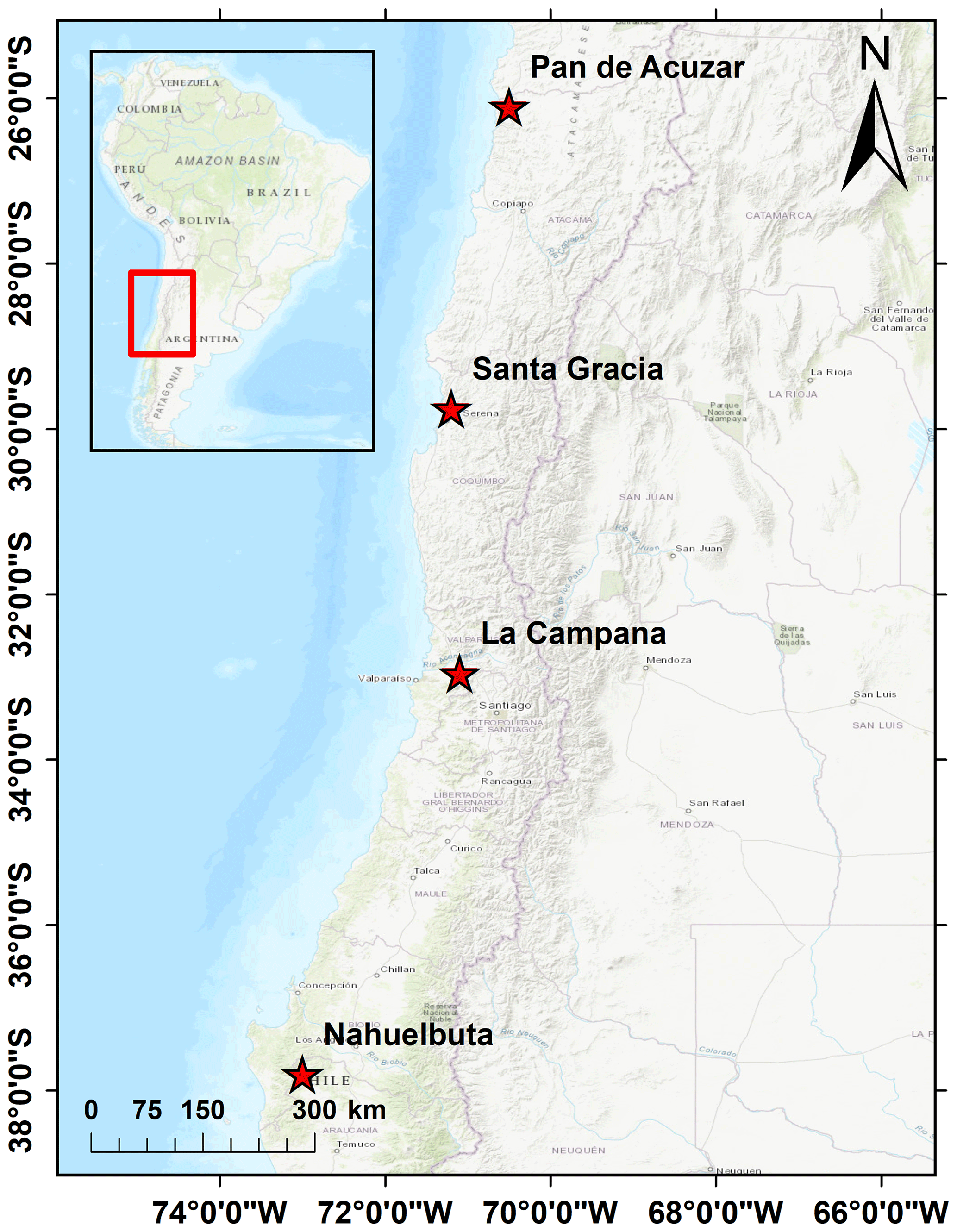
Figure 1Study areas in the Coastal Chilean Cordillera ranging from an arid environment in the north (Pan de Azúcar) to a semi-arid (Santa Gracia), Mediterranean (La Campana), and humid–temperate environment in the south (Nahuelbuta). The above map is obtained from the Environmental System Research Institute (ESRI) map server (https://services.arcgisonline.com/ArcGIS/rest/services/World_Topo_Map/MapServer, last access: 25 April 2022).
This section summarizes the geologic, climate, and vegetation settings of the four selected catchments (Fig. 1) investigated in the Chilean Coastal Cordillera. These catchments (from north to south) are located in the Pan de Azúcar National Park (arid, ∼ 26∘ S), Santa Gracia Nature Reserve (semi-arid, ∼ 30∘ S), and La Campana (Mediterranean, ∼ 33∘ S) and Nahuelbuta (temperate–humid, ∼ 38∘ S) national parks. Together, these study areas span ∼ 1300 km of the Coastal Cordillera. These study areas are chosen for their steep climate and ecological gradient from north (arid environment with small to no shrubs) to south (humid–temperate environment with evergreen mixed forests) (Schaller et al., 2020). The study areas are part of the German–Chilean priority research program EarthShape (https://www.earthshape.net, last access: 10 August 2022) and ongoing research efforts within these catchments.
The bedrock of the four study areas is composed of granitoid rocks, including granites, granodiorites, and tonalites in Pan de Azúcar, La Campana, and Nahuelbuta, respectively, as well as gabbro and diorites in Santa Gracia (Oeser et al., 2018). The soil types in each catchment were identified as a sandy loam in three northern catchments (with high bulk density: 1300–1500 kg m−3) and sandy clay loam in Nahuelbuta (with lower bulk density: 800 kg m−3) (Bernhard et al., 2018). The western margin of Chile along the latitudes of the different study areas is characterized by a similar tectonic setting where an oceanic plate (currently the Nazca Plate) has been subducting under the South American Plate since the Paleozoic. Despite this common tectonic setting, slight differences in modern rock uplift rates are documented in the regions surrounding the three northern catchments (i.e., < 0.1 mm yr−1 for ∼ 26 to ∼ 33∘ S) (Melnick, 2016) and the southern catchment (i.e., 0.04 to > 0.2 mm yr−1 for ∼ 38∘ S over the last 4 ± 1.2 Myr) (Glodny et al., 2008; Melnick et al., 2009). Over geologic (millennial) timescales, measured denudation rates in the region range between ∼ 0.005 and ∼ 0.6 mm yr−1 (Schaller et al., 2018). As this study focuses on the sensitivity of topography to seasonal variations in vegetation and precipitation change, the tectonic parameters (rock uplift) specific to each study areas are held constant. Given this, we assume a uniform rock uplift rate of 0.05 mm yr−1 for results presented here. This rate is broadly consistent with the range of previously reported values.
The climate gradient in the study areas ranges from an arid climate in Pan de Azúcar (north) with mean annual precipitation (MAP) of ∼ 11 mm yr−1 to semi-arid in Santa Gracia (MAP: ∼ 88 mm yr−1), a Mediterranean climate in La Campana (MAP: ∼ 350 mm yr−1), and a temperate–humid climate in Nahuelbuta (south) with a MAP of 1400 mm yr−1 (Ziese et al., 2020). The observed mean annual temperatures (MATs) also vary with latitude, ranging from ∼ 20 ∘C in the north to ∼ 5 ∘C in the south (Übernickel et al., 2020). The previous gradients in MAP and MAT as well as latitudinal variations in solar radiation result in a southward increase in vegetation density (Bernhard et al., 2018). The vegetation gradient is evident from mean MODIS Normalized Difference Vegetation Index (NDVI) values ranging from ∼ 0.1 in Pan de Azúcar (north) to ∼ 0.8 in Nahuelbuta (south) (Didan, 2015). In this study, NDVI values are used as a proxy for vegetation cover density, similar to the approach of Schmid et al. (2018). However, one of the major limitations of using NDVI is that the values are saturated when the ground is covered by shrubs or larger broad-leaved forests in regions with high biomass (Van Der Meer et al., 2001) (e.g., the catchment in the humid–temperate setting). This may have implications for the shear stress partitioning ratio used to estimate the sediment and bedrock erodibilities (see Eqs. 10–13), as the NDVI values for shrub-covered land and a mature forest could be similar in such cases (Huang et al., 2021).
This gradient in climate and vegetation cover from north to south in the Chilean Coastal Cordillera provides an opportunity to study the effects of seasonal variations in vegetation cover and precipitation on catchment-scale erosion rates in different climate settings.
3.1 Data used for model inputs
This study focuses on predicting and comparing the average responses in catchment erosion that occur over seasonal timescales with variable precipitation and vegetation cover. However, erosion in arid and semi-arid regions can vary on sub-seasonal timescales due to high-intensity storms occurring over timescales of a couple of hours or days. Hence, the model does not capture the role of extreme precipitation events. Also, our preliminary modeling results suggest that the relationship between vegetation cover and erosion rates may be affected by inherited simulated slope values from the previous season, which may lead to a blended signal in the output.
Initial topography for the four selected catchments was obtained by cropping the SRTM digital elevation model (DEM) in rectangular shapes encapsulating the catchment of interest (Fig. 1). These catchments are the same as those investigated with previous soil, denudation, and geophysical studies within the EarthShape project (e.g., Bernhard et al., 2018; Oeser et al., 2018; Schaller et al., 2018; Dal Bo et al., 2019). The DEM has a spatial resolution of 90 m and is the same as the cell size used in the model (dx and dy) (SRTM dataset of Earth Resources Observation and Science – EROS – Center, 2017). The present-day total relief in the catchments is ∼ 1852 m in La Campana (∼ 33∘ S), ∼ 1063 m in Santa Gracia (∼ 30∘ S), ∼ 809 m in Nahuelbuta (∼ 38∘ S), and ∼ 623 m Pan de Azúcar (∼ 26∘ S). Investigated catchment sizes considered here vary between ∼ 64 km2 in Pan de Azúcar, ∼ 142.5 km2 in Santa Gracia, ∼ 106.8 km2 in La Campana, and ∼ 68.7 km2 in Nahuelbuta. We note that present-day topography as the initial condition in simulations can introduce an initial transience in erosion rates due to assumed model erosional parameters (e.g., erodibility, hillslope diffusivity) differing from actual parameters within the catchment. We address this issue through a detrending of model results described later (see Sect. 3.6). Furthermore, the inherent timescales at which the topography and surface processes respond (depicted by LEMs) are dependent on the physical properties incorporated and the model forcings (such as rock uplift), all of which have uncertainties associated with them. Hence, it is unlikely that the SRTM DEM used for the initial condition is in equilibrium. Given this, the detrending of our time series of results to remove long-term transience aids in identifying seasonal transients in precipitation and vegetation cover.
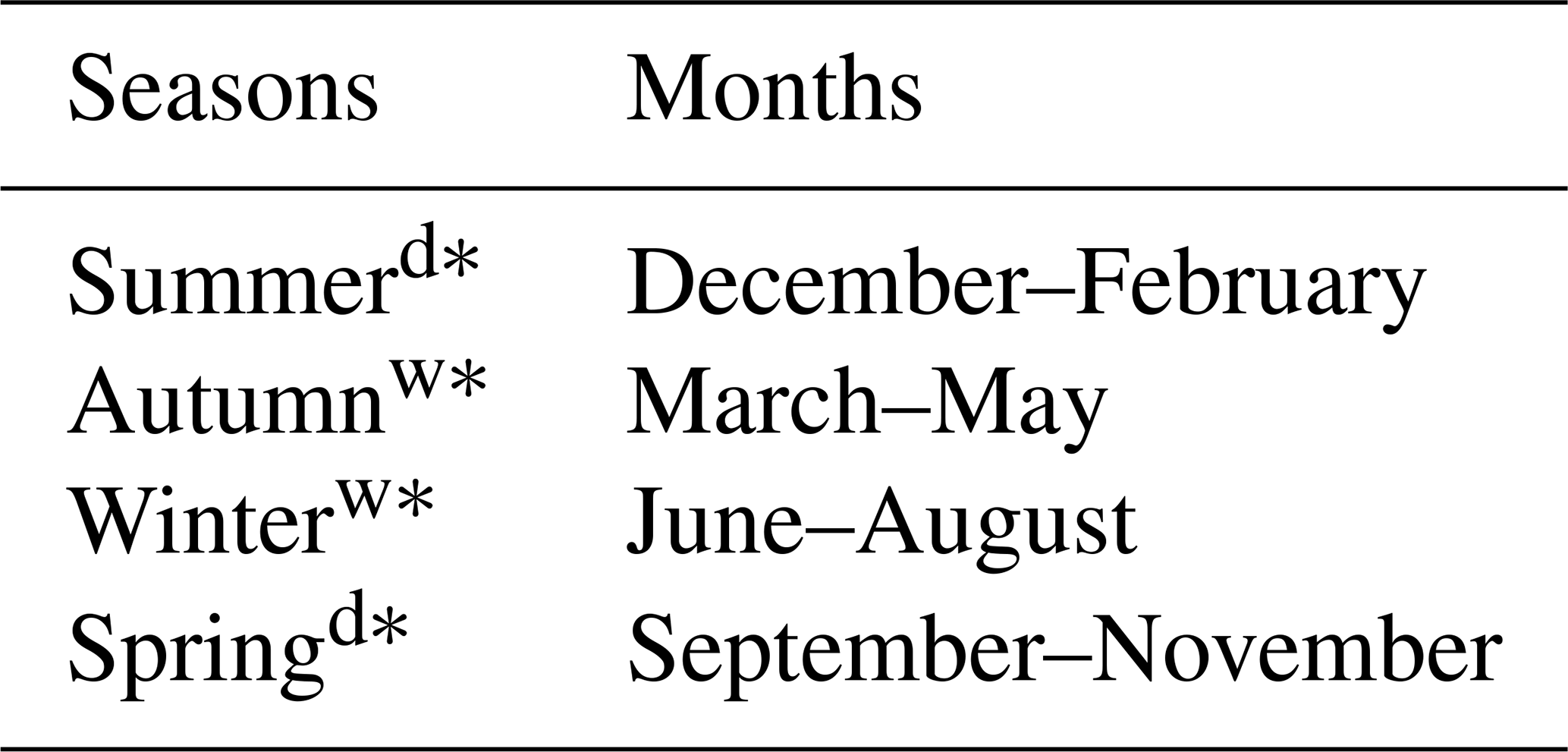
Precipitation data used over each study area (Fig. 3b) were acquired from the GPCC for the period 1 March 2000 to 31 December 2019 (DD/MM/YEAR). The data have a spatial resolution of 1∘ and a 1 d temporal resolution and comprise daily land surface precipitation from rain gauges built on historic data and data from the Global Telecommunication System (Ziese et al., 2020). The previous data were augmented with daily precipitation weather station data from 1 to 28 February 2020 obtained from Übernickel et al. (2020). We do this to include all the seasons between 2000 and 2019, i.e., from the austral autumn of 2000 to the austral summer of 2019. The periods (months of a year) of specific seasons in the Chilean Coastal Cordillera are given in Table 1. Seasonal precipitation rates were calculated by summing daily precipitation rates at 3-month intervals. The seasonality and intensity of precipitation in the wet season (winter) increase from the arid (Pan de Azúcar) to humid–temperate (Nahuelbuta) region.
Table 1Months of a year corresponding to specific seasons in the Chilean Coastal Cordillera.
* The notation is “d” for dry season and “w” for wet season.
NDVI derived from remote sensing imagery has proven to be an effective tool to estimate seasonal changes in vegetation cover density (Garatuza-Payán et al., 2005). Normalized Difference Vegetation Index (NDVI) values were obtained from MODIS (Didan, 2015) satellite data and were used as a proxy for changes in vegetation cover in the catchments. However, the major limitation of the conversion of NDVI to vegetation cover includes a saturation problem in NDVI values that occurs in high-biomass regions such as our humid–temperate setting (Huete et al., 2002). This saturation can occur if the ground is covered by shrubs, at which point the information on different plant communities for associated erosion-relevant properties is lost (e.g., rooting depth). The effect of a saturation in NDVI values could lead to uncertainties in calculating the shear stress partitioning ratio (see Eqs. 10–11), consequently affecting estimates of erodibility (see Eqs. 12–13). This is potentially important for humid–temperate climate settings characterized by high NDVI values (i.e., > 0.8). The NDVI data were acquired for 20 years (1 March 2000–28 February 2020), with a spatial resolution of 250 m and temporal resolution of 16 d. For application within the model simulations, the vegetation cover dataset was resampled using the nearest-neighbor method to match the spatial resolution (90 m) of the SRTM DEM and temporal resolution of 3 months. To summarize, seasonal variations in precipitation rate and vegetation cover were applied to the simulations between 1 March 2000 and 28 February 2020 and encompass a 20-year record of observed variations in these factors.
Additional aspects of the catchment hydrologic cycle were determined using the following approaches for the same time period previously mentioned. First, evapotranspiration (ET) data were obtained from Global Land Data Assimilation System (GLDAS) Noah version 2.1, with a monthly temporal resolution and spatial resolution of 0.25∘ (∼ 28 km) (Beaudoing et al., 2020; Rodell et al., 2004). The data were obtained from March 2000 to February 2020. Due to the coarse resolution of the dataset, ET is assumed to be uniform over the entire catchment area. No higher-resolution datasets were available over the 20-year time period of interest.
Soil properties such as the grain size distribution (sand, silt, and clay fraction) and bulk density were adapted from Bernhard et al. (2018) to estimate soil water infiltration capacity in each study area. Based on these soil properties, the soils have been classified as a sandy loam (in Pan de Azúcar, Santa Gracia, and La Campana) and sandy clay loam (Nahuelbuta). Average bulk density values of 1300, 1500, 1300, and 800 kg m−3 were used for Pan de Azúcar, Santa Gracia, La Campana, and Nahuelbuta, respectively (Bernhard et al., 2018).
Figure 2 shows correlations of the model input data, such as variable climatic or hydrologic cycle metrics (i.e., precipitation and evapotranspiration) and vegetation cover for the climate zone of each study area investigated, with other variables such as topography and soil texture. The relationships shown for each study area in different climate and ecological zones are based on the 20 years of data used (i.e., autumn of 2000–summer of 2019). The relationship between fractional vegetation cover (V) and evapotranspiration (ET) indicates a slightly positive trend in the semi-arid setting (Fig. 2a), whereas the relationship in the Mediterranean setting is a steep positive gradient, with low vegetation cover (0.4–0.55) and evapotranspiration (i.e., 50–100 mm season−1) in the winter, which increases in summer (90–160 mm season−1) in response to vegetation growth (i.e., V= 0.55–0.65). Similar trends in V and ET are indicated in the humid–temperate setting during the summer with V in the range of 0.55–0.75 and ET ranging between 150 and 350 mm season−1. However, during winters, even after high V in the humid setting, lower values in ET are reported, with a positive trend. To help understand the datasets of precipitation (P) with ET, a Budyko curve is presented in Fig. 2b, where the actual ET (AET) and potential ET (PET) are normalized by P. In Fig. 2b most the data points from the humid–temperate setting are above the energy limit and indicate high soil water infiltration during summer seasons. Also, data points above the water limit (blue line in Fig. 2b) indicate a carry-over in soil moisture from a wet season to a few dry seasons in the humid, Mediterranean, and semi-arid settings.
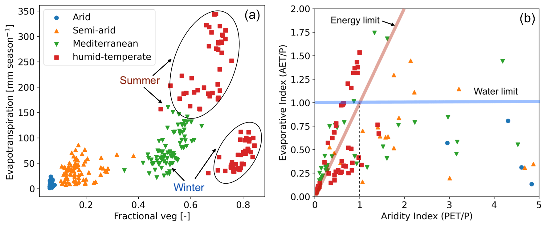
Figure 2Parameter correlation for observations used as model input data (i.e., seasonal precipitation, vegetation cover, and evapotranspiration) including (a) fractional vegetation cover (derived from NDVI) and evapotranspiration (derived from GLDAS Noah), as well as (b) a Budyko curve representing the relationship between precipitation (P), potential evapotranspiration (PET), and actual transpiration (AET). The points above the water limit (blue line) indicate the contribution of soil moisture to ET. The seasons (points) above the energy limit (red line) indicate the precipitation loss by infiltration. The plots represent observations corresponding to autumn of 2000 to summer of 2019. Each data point represents one season, and points are color-coded by the climate of the study areas. See Sect. 3.1 for a description of the datasets used.
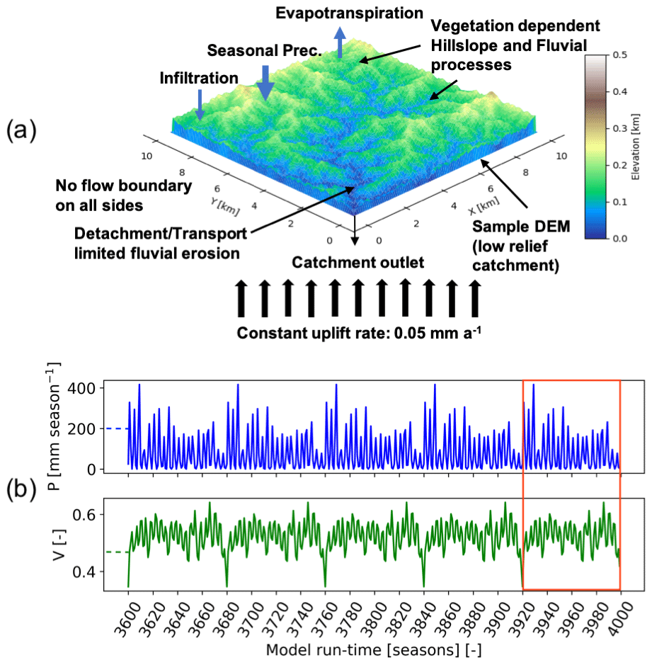
Figure 3Schematic of the model geometry as well as the seasonal precipitation and vegetation forcings used in this study. (a) Model setup representing a sample DEM (low-relief catchment) with no-flow boundaries on all sides and a single catchment outlet. The model involves vegetation-dependent seasonal hillslope and fluvial processes as well as rainfall–infiltration–runoff modeling. (b) Seasonal precipitation and vegetation cover dataset (Mediterranean setting in La Campana) for the last five iterations of model simulations. The results of highlighted iterations (after detrending for long-term transients) are analyzed in consecutive sections.
3.2 Model setup
We applied the Landlab landscape evolution model, a Python-based modeling toolkit (Hobley et al., 2017), combined with the SPACE 1.0 model (Shobe et al., 2017). The SPACE model allows coupled detachment- and transport-limited fluvial processes with simultaneous bedrock erosion as well as sediment entrainment and deposition. The Landlab–SPACE programs were applied using a set of runtime scripts and input files (Sharma and Ehlers, 2023) to account for vegetation and climate change effects on catchment erosion (i.e., fluvial erosion and hillslope diffusion) using the approach described in Schmid et al. (2018) and Sharma et al. (2021). In addition, the geomorphic processes considered involve infiltration of surface water into soil (Rengers et al., 2016) based on the Green–Ampt method (Green and Ampt, 1911) and runoff modeling. The constitutive equations for the processes involved in the model simulations are presented in Sect. 3.3.
The model parameters (Table A1 in Appendix) are selected for the distinct climate and ecological settings in the Chilean Coastal Cordillera based on the observations presented by Schaller et al. (2018), Bernhard et al. (2018), and Übernickel et al. (2020). The model state parameters (i.e., erodibility, diffusivity, rock uplift rate, etc.) in the simulations are adapted from Sharma et al. (2021). The parameters pertaining to the effect of vegetation cover on erosion rates (e.g., Manning's number for bare soil and reference vegetation cover) are adapted from Schmid et al. (2018). The model was simulated at a seasonal scale (time step of 3 months) from the autumn of 2000 (1 March 2000) to the summer of 2019 (28 February 2020). Simulations were conducted for a total of 1000 years with a time step of one season (3 months) with 20 years (2000–2019) of observations in vegetation and precipitation. These 20 years of observations were repeated (looped) 50 times to identify and detrend long-term transient trends in catchment erosion rates due to potential differences in actual and assumed erosional parameters such as the hillslope diffusivity or fluvial erodibility. The combined effects of temporally variable (at seasonal scale) precipitation and vegetation cover (also spatially variable) on catchment-scale erosion rates are therefore the primary factors influencing predicted erosion rates.
3.3 Implementation of vegetation-dependent hillslope and fluvial processes in Landlab components
This section includes the description of vegetation-dependent hillslope and fluvial erosion routines defined in the Landlab components used in this study. Our approach is based on previous work by Istanbulluoglu (2005), Schmid et al. (2018), and Sharma et al. (2021).
3.3.1 Vegetation-dependent hillslope processes
The rate of change in topography due to hillslope diffusion (Fernandes and Dietrich, 1997) is defined as follows:
where qs is sediment flux along the slope S at a time step (where dt is one season) in a grid cell. We applied a slope- and depth-dependent linear diffusion rule following the approach of Johnstone and Hilley (2014) such that
where Kd is diffusion coefficient [m2 season−1], d* is sediment transport decay depth [m], and H denotes sediment thickness in a grid cell at a particular time step. In the model, the diffusion coefficient is dependent on vegetation cover present on hillslopes, which is estimated following the approach of Istanbulluoglu (2005), as follows:
where Kb is the diffusivity for bare soil [m2 season−1] and α represents the exponential decay coefficient (see Table A1 in the Appendix). The vegetation cover fraction in a grid cell is denoted by V.
3.3.2 Vegetation-dependent fluvial processes
The fluvial erosion is estimated for a two-layer topography (i.e., bedrock and sediment are treated explicitly) in the coupled detachment- and transport-limited model, SPACE 1.0 (Shobe et al., 2017). Bedrock erosion and sediment entrainment are calculated simultaneously in the model in each grid cell. The total fluvial erosion is defined as
where the left-hand side denotes the total fluvial erosion rate. The first and second terms on the right-hand side denote the bedrock erosion rate and sediment entrainment rate.
The rate of change in the height of bedrock R per unit time [m season−1] is defined as
where Er [m season−1] is the volumetric erosion flux of bedrock per unit bed area. The previous equation implies that the topography adjusts to the rock uplift rates. As a result, if model-prescribed erosional parameters differ from those of the modern (actual) topography used for the initial condition, then a transience would occur until an equilibrium is reached between the prescribed parameters and the rock uplift rate. In practice, we found the effect of this induced transience to be small, but we mitigated the effect through a linear detrending (see Sect. 3.6).
The sediment thickness is updated in each grid cell at a time step such that the change in sediment thickness H [m] is defined as a fraction of net deposition rate and solid fraction sediments, which is expressed as
where Ds [m season−1] is the deposition flux of sediment, Es [m season−1] is volumetric sediment entrainment flux per unit bed area, and φ is the sediment porosity. The porosity in each study area is calculated from the bulk density estimations of Bernhard et al. (2018), which ranges from 0.43 in the semi-arid to 0.7 in the humid–temperate settings (see Table A1).
Following the approach of Shobe et al. (2017), Es and Er are expressed as follows:
where Ks [m−1] and Kr [m−1] are the sediment erodibility and bedrock erodibility parameters, respectively. The threshold stream power for sediment entrainment and bedrock erosion is denoted as ωcs [m season−1] and ωcr [m season−1] in the above equations. Bedrock roughness is denoted as H* [m] and the term corresponds to the soil production from bedrock. With higher bedrock roughness magnitudes, more sediment would be produced.
Ks and Kr were modified in each time step in the model simulations by introducing the effect of Manning's roughness to quantify the effect of vegetation cover on bed shear stress in each model grid cell:
where ρw [kg m−3] and g [m s−2] are the density of water and acceleration due to gravity, respectively. Manning's numbers for bare soil and vegetated surface are denoted as ns and nv. Ft represents the shear stress partitioning ratio. Manning's number for vegetation cover and Ft are calculated as follows:
where nvr is Manning's number for the reference vegetation. Here, Vr is reference vegetation cover (i.e., V= 100 %), V is local vegetation cover in a model grid cell, and w is the empirical scaling factor.
By combining the stream power equation (Tucker et al., 1999; Howard, 1994; Whipple and Tucker, 1999) and above concept of the effect of vegetation on shear stress, we define modified sediment and bedrock erodibility parameters, following the approach of Schmid et al. (2018) and Sharma et al. (2021), which are as follows:
where Kvs [m−1] and Kvr [m−1] are modified sediment and bedrock erodibilities, respectively. These are influenced by the fraction of vegetation cover V in each grid cell at time step. Hence, Ks and Kr in Eqs. (7) and (8) are replaced by Kvs and Kvr in the model to account for vegetation-dependent fluvial erosion. The trends of Kd, Kvs, and Kvr are illustrated in Fig. 3 in Sharma et al. (2021).
3.3.3 Vegetation-dependent soil water infiltration
The soil water infiltration rate is estimated by applying the Green–Ampt equation (Green and Ampt, 1911; Julien et al., 1995), which is as follows:
where f(t) is the infiltration rate [m s−1] at time t, Ke is the effective hydraulic conductivity [m s−1], F is the cumulative infiltration [m], Ψ is the suction at the wetting front [m], and Δθ is the difference between saturated and initial volumetric moisture content [m3 m−3]. Effective hydraulic conductivity is highly variable and anisotropic; hence, it was considered to be uniform with a value of m s−1 for each catchment.
Following the approach of Istanbulluoglu and Bras (2006) for loamy soils, the soil water infiltration was modified to account for variable vegetation cover in each grid cell, as follows:
where Ic is the infiltration capacity and V is the vegetation cover (between 0 and 1) in a model grid cell at time step t. Values used in the simulations for the parameters in Eqs. (14)–(16) are provided in Appendix Table A1.
3.3.4 Estimation of runoff rates
The precipitation rates [m season−1] are subjected to soil water infiltration [m season−1] and evapotranspiration [m season−1] to estimate the seasonal runoff rates [mm season−1]. The runoff rates (R) at every time step (t) are calculated using the actual soil water infiltration (Ia) and the actual evapotranspiration (ET) as follows:
where P is the precipitation amount in a season. This relationship was applied in the model grid cells with nonzero sediment thickness, which is updated at each time step (see Eq. 6) in order to facilitate infiltration. If the sediment is not present in the grid cell, there is no soil water infiltration. As ET is the input parameter, there may be instances of higher ET than P in the summer seasons in the humid, Mediterranean, and semi-arid settings. This is evident in Fig. 2b where the minimum of both values is used as ET in the given time step.
3.4 Boundary and initial conditions
The boundaries are closed (no flow) on all sides, with a single stream outlet at the point of minimum elevation at a boundary node (Fig. 3). In contrast to previous modeling studies (Schmid et al., 2018; Sharma et al., 2021) in the same study areas, we used present-day topography as the initial condition in each study area for simulations instead of a synthetic topography produced during a model spin-up phase in Landlab. This implies four different initial conditions for four study areas, such as topography, climate, vegetation, sediment thickness, and porosity. Initial sediment cover thickness is considered uniform across the model domain and was approximated based on observations presented in Schaller et al. (2018) and Dal Bo et al. (2019). The sediment thicknesses used are 0.2 m in the arid (AZ), 0.45 m in semi-arid (SG), 0.6 m in the Mediterranean (LC), and 0.7 m in humid–temperate (NA) catchments. The rock uplift rate is kept constant throughout the entire model run as 0.05 mm yr−1, adapted from a similar study (Sharma et al., 2021). However, in a 1000-year simulation, differences in base-level (rock uplift) effects have a limited impact on the variations in results interpreted here.
3.5 Overview of simulations conducted
The simulations were designed to identify the sensitivity of erosion rates to seasonal variations in either precipitation rates or vegetation cover, as well as the more realistic scenario of coupled seasonal variations in both vegetation cover and precipitation. We evaluated this sensitivity with the following three scenarios.
-
Scenario 1. Influence of constant (mean seasonal) precipitation with seasonal variations in vegetation cover on catchment-scale erosion rates.
-
Scenario 2. Influence of seasonal variation in precipitation and constant (mean seasonal) vegetation cover on catchment-scale erosion rates.
-
Scenario 3. Influence of coupled seasonal variations in both precipitation and vegetation cover on catchment-scale erosion rates.
The results for scenarios 1–3 are illustrated in Sect. 4.1, 4.2, and 4.3, respectively.
3.6 Detrending of results for long-term transients
Model simulations were conducted for 1000 years using 20 years (March 2000–February 2020) of observations in vegetation cover and precipitation and were repeated 50 times for a total simulation duration of 1000 years. Simulations presented here were conducted on the present-day topography, which was updated at each time step in the LEM (based on rock uplift rates and erosion) to allow for the application of observed time series of precipitation and vegetation change in different ecosystems and study areas. This choice of setting comes with the compromise that the erosional parameters (e.g., diffusivity, erodibility) used in the model (see Table A1 in the Appendix) are likely not the same as those that led to the present-day catchment topography. As a result, a long-term transient in erosion rates is expected as the model tries to reach an equilibrium with assumed erosional parameters. To correct for any long-term transients in erosion influencing our interpretations, we conducted a linear detrending of the results to remove any long-term variations. The detrending was conducted through a linear regression over entire time series of 1000 years, and the values were corrected using the slope of the regression line. Hence, the detrended model results for the last 20 years are analyzed and discussed in Sects. 4 and 5. In practice, the detrending of time series did not impart a significant change to the results presented.
In the following sections, we focus our analysis on the mean catchment erosion rates over seasonal (3 months) timescales (see Table 1). In all scenarios, the rock uplift rate was kept constant at 0.05 mm yr−1 following the approach of Sharma et al. (2021). For simple representation, the results of the last 5 years of the last cycle of transient simulations starting from autumn 2015 to summer 2019 are displayed in Figs. 4, 6, and 8 (after detrending, see Sect. 3.6). The results for the entire time series (autumn 2000–summer 2019) are available in the Supplement (Figs. S1–S3). The precipitation and erosion rates are shown with the units millimeters per season [mm season−1].
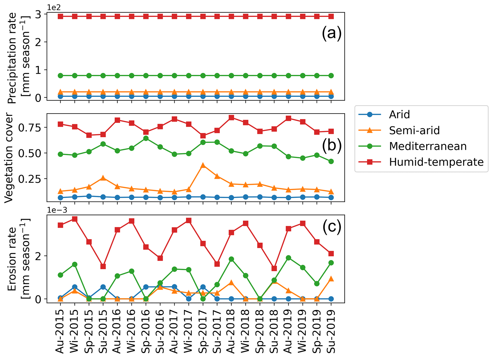
Figure 4Results of simulations with constant seasonal precipitation and variable vegetation over the last 5 years (autumn 2015–summer 2019) of the last cycle of the transient-state model run representing (a) mean catchment seasonal precipitation rates [mm season−1], (b) mean catchment seasonal vegetation cover [−], and (c) mean catchment seasonal erosion rates [mm season−1].
4.1 Scenario 1: influence of constant precipitation and seasonal variations in vegetation cover on erosion rates
In scenario 1, vegetation cover (MODIS NDVI from March 2000 to February 2020) fluctuates seasonally (Fig. 4b), and precipitation rates are kept constant at the seasonal mean (i.e., MAP divided by the number of seasons in a year) during the entire time series (Fig. 4a) (Ziese et al., 2020). The range of seasonal vegetation cover variations (and mean seasonal precipitation rates) is observed as 0.06–0.08 (3.92 mm season−1), 0.1–0.4 (20.16 mm season−1), 0.35–0.65 (79 mm season−1), and 0.5–0.85 (292 mm season−1) for the arid, semi-arid, Mediterranean, and humid–temperate settings, respectively (Fig. 4a–b). The predicted mean catchment seasonal erosion rates range from 0–6 , 0–9.4 , 0–2.3 , and – mm season−1 for the arid, semi-arid, Mediterranean, and humid–temperate settings, respectively (Fig. 4c).
To analyze the relationships between the relative changes in forcings and responses, seasonal changes in vegetation cover and erosion rates were normalized between 0 and 1 and plotted in Fig. 5a–d. An inverse relationship and negative correlation (Kendall τ correlation coefficient: 0.4–0.5) is visible between the normalized catchment erosion rates and vegetation cover for the dry season and wet season separately in the humid–temperate (Fig. 5d) and Mediterranean settings (Fig. 5c). The observed inversely linear relationship between vegetation and erosion changes in Mediterranean and humid–temperate settings demonstrates the prevalence of fluvial (water-driven) and overland flow processes within these catchments, with hillslope diffusion playing a negligible role. In contrast, no correlation was found for the arid and semi-arid settings.
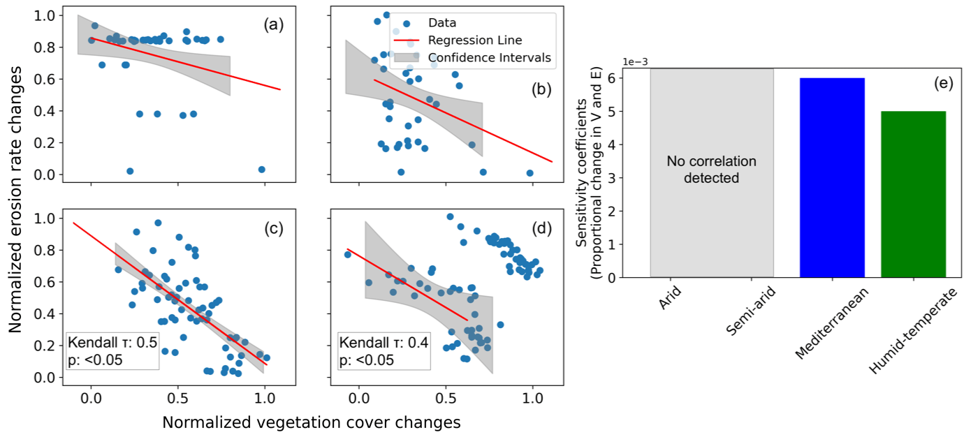
Figure 5Seasonal changes (normalized) in vegetation cover and erosion rates for the scenario with constant precipitation and seasonal changes in vegetation cover in the (a) arid, (b) semi-arid, (c) Mediterranean, and (d) humid–temperate settings, with the information on confidence interval (grey shading) and Kendall τ correlation coefficients. (e) Sensitivity coefficients for proportional changes in vegetation cover and erosion rates based on the slope and intercept of the regression lines for the above environmental settings. The sensitivity coefficient is defined as the slope of the regression line presented in panels (a)–(d).
The sensitivity coefficients based on the slope and intercept of the regression lines (Fig. 5a–d) are plotted in Fig. 5e. The results indicate a higher sensitivity of erosion rates to seasonal vegetation changes in the Mediterranean setting relative to the humid–temperate setting. However, in the arid and semi-arid settings, the lack of a significant correlation in the change in vegetation cover and erosion rates leads to a low sensitivity. This is due to very low mean precipitation rates (< 20 mm season−1) in the arid and semi-arid settings. The predicted erosion rates are relatively low (e.g., < 0.004 mm season−1) in this scenario due to low mean precipitation rates, which are primarily subjected to infiltration and evapotranspiration in these drier settings.
4.2 Scenario 2: influence of seasonal variations in precipitation and constant vegetation cover on erosion rates
In scenario 2, vegetation cover (MODIS NDVI from March 2000–February 2020) is kept constant at the mean seasonal vegetation cover (Fig. 6b) and precipitation rates vary seasonally (March 2000–February 2020) (Fig. 6a). The range of seasonal precipitation rate variations is observed as 0–32.42, 0–191.66, 0.03–417, and 26–987 mm season−1 in the arid, semi-arid, Mediterranean, and humid–temperate settings, respectively.
The simulated mean catchment seasonal erosion rates are observed in the range of , , , and mm season−1 in the arid, semi-arid, Mediterranean, and humid–temperate settings, respectively (Fig. 6c).
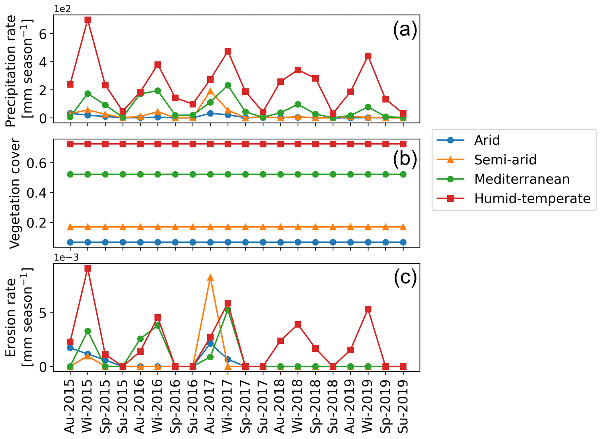
Figure 6Results of simulations with variable seasonal precipitation and constant vegetation over the last 5 years (autumn 2015–summer 2019) of the last cycle of the transient-state model run representing (a) mean catchment seasonal precipitation rates [mm season−1], (b) mean catchment seasonal vegetation cover [−], and (c) mean catchment seasonal erosion rates [mm season−1].
Similar to scenario 1, the changes in seasonal precipitation and erosion rates are normalized between 0 and 1 and plotted in Fig. 7a–d. A strong positive correlation (Kendall τ correlation coefficient ranging from 0.5 in semi-arid to 0.9 in Mediterranean and humid–temperate settings) in the normalized precipitation and erosion rate changes is predicted with the majority of the data points within the 95 % confidence interval in all the settings. The sensitivity coefficients based on the proportional changes in precipitation and erosion rates indicate the highest sensitivity in semi-arid settings, with ∼ 5 %, ∼ 11 %, and ∼ 67 % lower sensitivities in the arid, Mediterranean, and humid–temperate settings, respectively (Fig. 7e). This may be due to occasional El Niño events with extremely high precipitation occurring in the arid and semi-arid settings (with sparse vegetation cover) in our study areas.
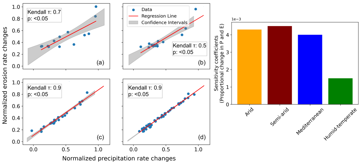
Figure 7Seasonal changes (normalized) in precipitation and erosion rates for the scenario with seasonal changes in precipitation rates and constant vegetation cover in the (a) arid, (b) semi-arid, (c) Mediterranean, and (d) humid–temperate settings, with the information on confidence interval (grey shading) and Kendall tau correlation coefficients. (e) Sensitivity coefficients for proportional changes in precipitation and erosion rates based on the slope and intercept of the regression lines for the above environmental settings. The sensitivity coefficient is defined as the slope of the regression line presented in panels (a)–(d).
4.3 Scenario 3: influence of coupled seasonal variations in both precipitation and vegetation cover on erosion rates
In this scenario, coupled variations in seasonal vegetation cover (MODIS NDVI from March 2000–February 2020) (Fig. 8b) and precipitation rates are presented for the years 2000–2019 (Fig. 8a). The range of seasonal precipitation rate (and seasonal vegetation cover, V) variations is 0–32.42 mm season−1 (V= 0.06–0.08), 0–191.66 (0.1–0.38), 0.03–417 (0.35–0.65), and 26–987 mm season−1 (0.5–0.85) in the arid, semi-arid, Mediterranean, and humid–temperate settings, respectively (Fig. 8a–b). The mean catchment seasonal erosion rates range from 0–2 , 0–1 , 0–1.4 , and 0–1.4 mm season−1 in the arid, semi-arid, Mediterranean, and humid–temperate settings, respectively (Fig. 8c).
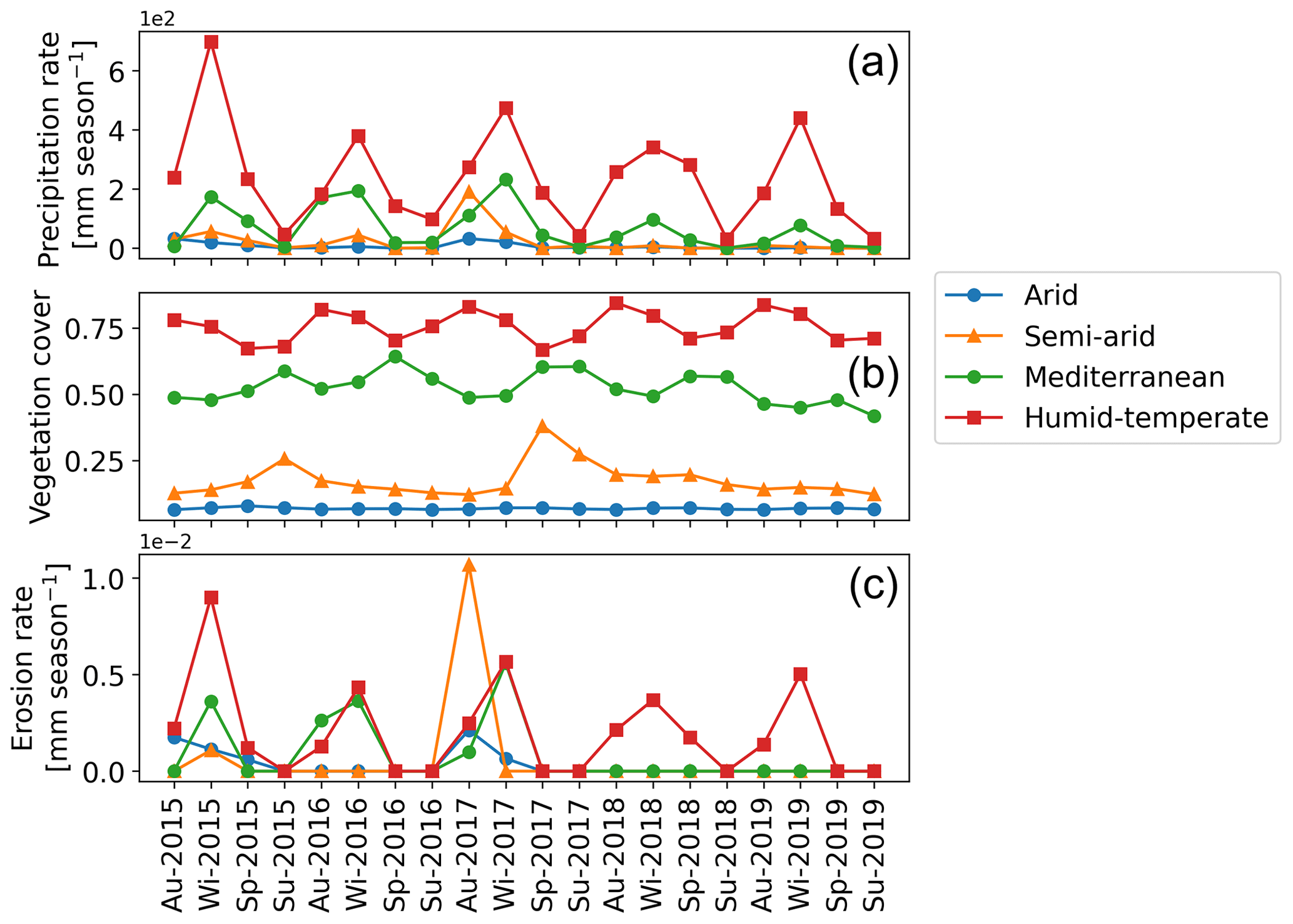
Figure 8Results of simulations with coupled variations in seasonal precipitation and vegetation over the last 5 years (autumn 2015–summer 2019) of the last cycle of the transient-state model run representing (a) mean catchment seasonal precipitation rates [mm season−1], (b) mean catchment seasonal vegetation cover [−], and (c) mean catchment seasonal erosion rates [mm season−1].
Changes in precipitation and erosion rates are normalized between 0 and 1 and plotted in Fig. 9a–d. Similar to the results from scenario 2, a strong positive correlation was predicted in all the environmental settings. The sensitivity coefficients based on the proportional changes in precipitation and erosion rates indicate the highest sensitivity in the semi-arid settings, with ∼ 25 % lower sensitivities in the arid and Mediterranean settings and ∼ 71 % lower sensitivities in the humid–temperate settings (Fig. 9e). Similarly, the isolated effect of changes in the vegetation cover on erosion rates (Fig. 10) does not yield a significant correlation in arid, semi-arid, and Mediterranean settings. However, we observe a strong negative correlation in the humid–temperate setting (Fig. 10d) during the wet season (Kendall tau correlation coefficient: −0.6, with > 95 % significance level). Hence, the sensitivity coefficients in this case are not plotted.
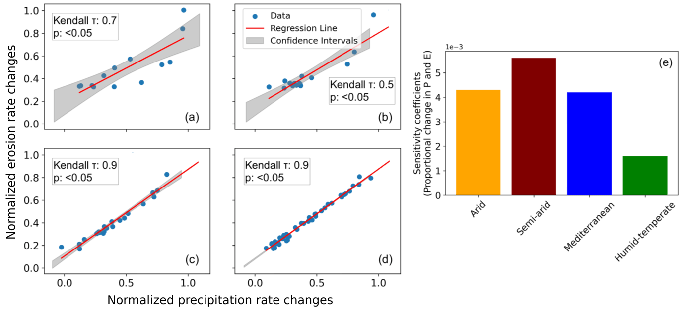
Figure 9Seasonal changes (normalized) in precipitation and erosion rates for the scenario with coupled seasonal changes in both precipitation rates and vegetation cover in the (a) arid, (b) semi-arid, (c) Mediterranean, and (d) humid–temperate settings, with the information on confidence interval (grey shading) and Kendall tau correlation coefficients. (e) Sensitivity coefficients for proportional changes in precipitation and erosion rates based on the slope and intercept of the regression lines for the above environmental settings. The sensitivity coefficient is defined as the slope of the regression line presented in panels (a)–(d).
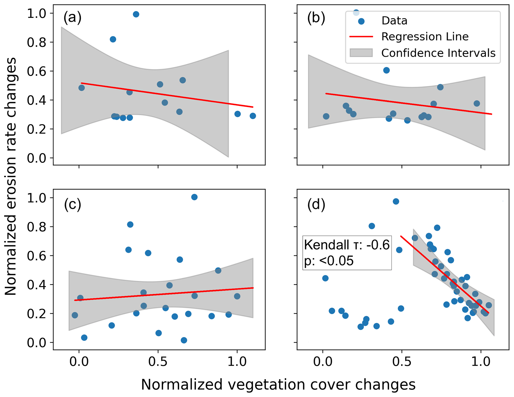
Figure 10Seasonal changes (normalized) in vegetation cover and erosion rates for the scenario with coupled seasonal changes in both precipitation rates and vegetation cover in the (a) arid, (b) semi-arid, (c) Mediterranean, and (d) humid–temperate settings, with the information on confidence interval (grey shading) and Kendall tau correlation coefficients.
The similarity in results obtained from scenarios 2 and 3 suggests a first-order control of seasonal precipitation changes on erosion rates (∼ 70 % higher sensitivity to changes in precipitation), with less significance to vegetation cover changes. For example, the sensitivity of erosion to precipitation rate changes in the semi-arid setting is predicted to be ∼ 70 % higher than that of the humid–temperate setting in both the scenarios.
5.1 Synthesis of the amplitude of change in erosion rates for model scenarios 1–3
The amplitude of change in mean catchment erosion rates (in percentage) varies at a seasonal scale (Fig. 11) between the study areas. The amplitude of change in erosion rates relative to their respective mean values was estimated (Fig. 11) using the coefficient of variation in percent (standard deviation divided by the mean of a dataset). The coefficient of variation is a statistical tool to compare multiple variables free from scale effects. It is a dimensionless quantity (Brown, 1998). This comparison represents the sensitivity of each catchment to changing seasonal weather for all three model scenarios (Sect. 4.1–4.3).
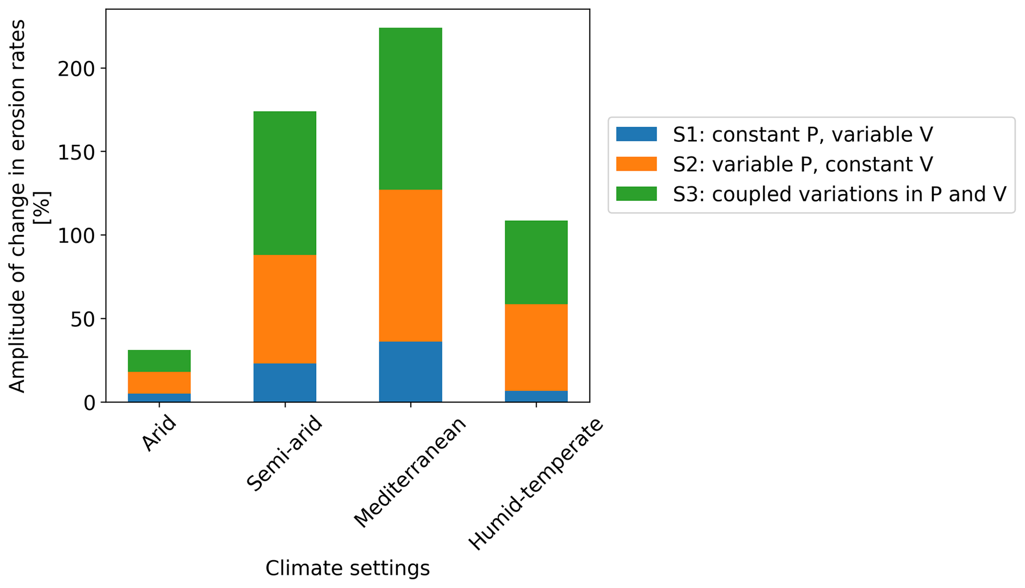
Figure 11Stacked bar plot depicting the amplitude of change in seasonal erosion rates (relative to their respective means). Scenario 1 is shown in blue and had variable vegetation cover and constant precipitation rates. Scenario 2 is shown in orange and had constant vegetation cover and variable precipitation rates, and scenario 3 is shown in green and represents the simulation with coupled variations in vegetation cover and precipitation rates.
In scenario 1, with seasonal variations in vegetation cover and constant seasonal precipitation (Fig. 11), the amplitude of change in erosion rates ranges between 5 % in the arid and 36 % in Mediterranean setting. The above results support the findings of Zhang et al. (2019), who used the soil and water assessment tool (SWAT) based on NDVI and climate parameters. They observed 20 %–30 % of the total change in sediment yield with constant precipitation and variable vegetation cover.
In scenario 2, with constant vegetation cover and variable precipitation rates (Fig. 11), the amplitude of change in erosion rates ranges from 13 % in the arid setting (AZ) to 52 %, 65 %, and 91 % in humid–temperate (NA), semi-arid (SG), and Mediterranean (LC) settings, respectively. A similar trend is observed in scenario 3 with coupled variations in vegetation cover and precipitation rates (Fig. 11), with the amplitude of change in erosion rates between 13 % in the arid setting and up to 50 %, 86 %, and 97 % in the humid–temperate, semi-arid, and Mediterranean settings, respectively. The magnitude of erosion rate changes is amplified in scenario 3, especially in the semi-arid setting (e.g., ∼ 21 % increase in the amplitude of change from scenario 2 to scenario 3). This amplification could be due to the 35 % change in vegetation cover in the semi-arid setting (Fig. 8). Overall, these observations indicate a high sensitivity of erosion in semi-arid and Mediterranean environments compared to arid and humid–temperate settings.
The pattern of erosion rate changes in scenarios 1–3 implies a dominant control of precipitation variations (rather than vegetation cover change) on catchment erosion rates at a seasonal scale. This interpretation is consistent with previous observational studies. For example, a field study by Suescún et al. (2017) in the Columbian Andes highlighted the significant influence of precipitation seasonality (over vegetation cover seasonality) on runoff and erosion rates. An observational catchment-scale study in the semi-arid Chinese Loess Plateau by Wei et al. (2015) indicated that intra-annual precipitation variations were a significant contributor to monthly runoff and sediment yield variations.
5.2 Synthesis of catchment erosion rates over wet and dry seasons
In this section, we discuss the ratio of seasonal precipitation and erosion rates to the mean annual precipitation (MAP) (Fig. 12a) and mean annual erosion (MAE) (Fig. 12b) during different seasons (i.e., autumn–summer) in a year, averaged over the last cycle of the transient simulations (i.e., depicting the erosion rate predictions for 2000–2019). These are defined as the ratio of the mean erosion (and precipitation) rates in a season (e.g., winter) to the mean annual erosion rates (and MAP) during the last 20 years of the transient simulations. This was done to identify the impact of precipitation during wet seasons (in this case, winter) in influencing the annual erosion rates. This analysis was performed for the simulation results of scenario 3 for different climate and ecological settings (i.e., arid to humid–temperate). We do this specifically with scenario 3 results to capture the trends in erosion rates with coupled variations in model input (i.e., precipitation and vegetation cover).
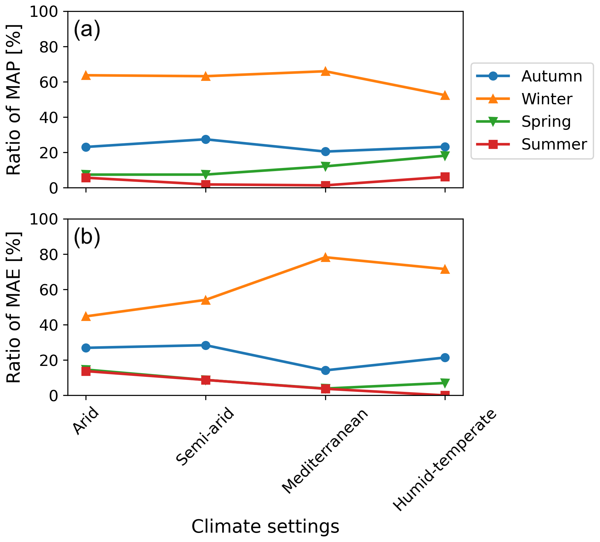
Figure 12The ratio of seasonal precipitation and erosion rates to mean annual precipitation (MAP) and mean annual erosion (MAE) during the last cycle of transient simulation results from scenario 3 (coupled seasonal variations in precipitation and vegetation cover). The plots correspond to (a) the ratio of MAP per season [%] and (b) the ratio of MAE per season [%]. Each color and point style represents the ratio for a distinct climate setting, i.e., arid, semi-arid, Mediterranean, and humid–temperate settings.
The values for the ratio of MAP during different seasons (Fig. 12a) depict winter (June–August) and summer (December–February) as the wettest and driest seasons of the year, respectively. For example, all study areas receive > 50 % and < 6 % of MAP during winters and summers. The same is reflected in Fig. 12b with 45 %, 55 %, 78 %, and 71 % of MAE in the arid, semi-arid, Mediterranean, and humid–temperate settings, respectively, during winters. On the contrary, during summers the share of MAE decreases from 14 % in the arid setting to 1 % in the humid–temperate setting. Autumn (March–May) receives lower precipitation amounts that range from 20 %–30 % of MAP in the study areas. Arid and semi-arid settings experience a relatively higher share of MAE (e.g., ∼ 30 %) than the Mediterranean and humid–temperate settings (e.g., ∼ 15 %–20 %). The spring season experiences relatively higher erosion rates despite a smaller share of MAP in arid and semi-arid settings. For example, the arid and semi-arid settings experience 10 %–14 % of the MAE for ∼ 7 % of MAP. At the same time, the Mediterranean and humid–temperate settings experience 5 %–7 % of MAE for ∼ 12 %–18 % of MAP during spring. Overall, we find that arid and semi-arid settings experience < 15 % and ∼ 50 % of MAE during the wet (winter) and dry (summer) seasons. The above relationship is amplified for the Mediterranean and humid–temperate settings with < 5 % and > 70 % of MAE occurring during wet and dry seasons, respectively. The latter is in agreement with an observational study by Mosaffaie et al. (2015) in a Mediterranean catchment in Iran. More specifically, Mosaffaie et al. (2015) used field observations from 2012–2013 to conclude that maximum erosion rates (> 70 %) are observed during the wet season, which decrease in the dry season (< 10 %).
5.3 Consideration of transient sediment dynamics in model results
This section discusses the impact of lag times from when sediment is eroded from a source area until it leaves the catchment outlet. This analysis was conducted because in natural systems, when sediment is eroded from its source, it takes time to leave the catchment (in this case the model domain) and be recorded as eroded in our analysis. According to field studies and modeling experiments, this time lag is usually more than a season (i.e., 3 months) (e.g., Buendia et al. 2016). Also, these time lags are dependent on the morphology of the catchment in addition to the geology, climate, and vegetation cover of the area. Hence, the simulation results (of scenario 3 with coupled variations in seasonal precipitation and vegetation cover) for the catchments in the Mediterranean (Fig. 13a) and humid–temperate settings (Fig. 13b) are compared. We do this to capture the topological influence on lag times, as both the catchments have different topographies and surface area. The time lags in precipitation, erosion, and concentration of sediment leaving the catchment outlet are analyzed and presented in Fig. 13. The concentration of sediment is defined as a dimensionless quantity () estimated from sediment flux (Qs) and discharge rates (Q) at the catchment outlet at a particular time step in the model simulation.
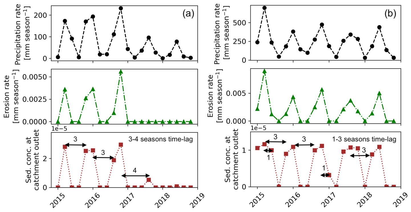
Figure 13Simulation results (scenario 3: coupled variations in precipitation in vegetation cover) to capture the time lags in precipitation, erosion rates, and sediment concentration at the catchment outlet over the last 5 years (autumn 2015–summer 2019) of the last cycle of the transient-state model run for the catchments in the (a) Mediterranean and (b) humid–temperate setting.
In the Mediterranean settings, these time lags range from three to four seasons and are relatively large (e.g., from wet season 2016 to wet season of 2017, see Fig. 13a), despite high channel relief of 1800 m. This signal is also blended due to the relatively large surface area of the catchment (i.e., 106 km2). However, in the humid–temperate setting, these time lags range from one to three seasons (Fig. 13b) with relatively lower channel relief (i.e., 800 m) and smaller catchment area (i.e., 69 km2). Hence, the time lags in the study areas are dominated by changes in vegetation cover as well as precipitation magnitude and frequency in the region with minimal influence of topology of the catchment. This is due to the primary influence of vegetation and precipitation modulations rather than the base-level changes in the catchment topology on the lag times in sediment dynamics. In the catchments in both these climate settings, the pulse of sediment leaving the catchment is evenly distributed, with the maximum concentration of sediment leaving the catchment in the same wet season when it is eroded from its source. These time lags would result in enhanced sensitivity of the proportional changes in erosion rates to the changes in seasonal precipitation and (or) vegetation cover, as the sediment is transported even in seasons when the sediment is not eroded from its source (e.g., wet season in 2017 in both of the above climate settings). This poses a limitation to the current study and is revisited in the model limitations (Sect. 5.5).
5.4 Comparison to previous studies
In this section, we relate the broad findings of this study to previously published observational studies. In an observational study in an agrarian drainage basin in the Belgian Loam Belt, Steegen et al. (2000) evaluated sediment transport over various timescales (including seasonal). They observed lower sediment fluxes during the seasons with high vegetation cover. In addition, an observational study by Zheng (2006) investigated the effect of vegetation changes on soil erosion in the Loess Plateau, China, and concluded that soil erosion was significantly reduced (up to ∼ 50 %) after vegetation restoration. Another observational study in semi-arid grasslands in the Loess Plateau, China, by Hou et al. (2020) highlighted a considerable reduction in erosion rates due to the development of richness and evenness of the plant community in the early to the middle wet season. Our results from scenario 1 (seasonal variations in vegetation cover with constant precipitation rates) support the findings of the above studies whereby a negative correlation (Kendal τ: −0.4– −0.5) was found between vegetation cover and erosion rates in humid–temperate and Mediterranean settings (see Fig. 5).
A catchment-scale observational study in Baspa Valley, NW Himalayas (Wulf et al., 2010), analyzed seasonal precipitation gradients and their impact on fluvial erosion using weather station observations (1998–2007). The study observed a positive correlation between precipitation and sediment yield variability, demonstrating the summer monsoon's first-order control on erosion processes. An observational study by Wei et al. (2015) in the Loess Plateau, China, evaluated erosion and sediment transport under various vegetation types and precipitation variations. They found that significant changes in landscape pattern and vegetation coverage (i.e., land use and land cover) might contribute to long-term dynamics of soil loss. However, seasonal variations in runoff and sediment yield were mainly influenced by rainfall seasonality. In comparison to the results of this study, we find the similarity in the patterns of erosion rates in scenario 2 (variable precipitation and constant vegetation cover) and scenario 3 (coupled variations in precipitation and vegetation) to be consistent with the findings of Wei et al. (2015). For example, the amplitude of change in erosion rates (Fig. 10) in scenarios 2 and 3 differs by 0 %, 6 %, and −2 % in the arid, Mediterranean, and humid–temperate settings, respectively. However, this difference is enhanced in the semi-arid region (i.e., ∼ 23 %) due to a relatively high degree of variation (∼ 25 %) in seasonal vegetation cover change.
Finally, an observational study in the Columbian Andes by Suescún et al. (2017) assessed the impact of seasonality on vegetation cover and precipitation and found higher erosion rates in regions with steeper slopes. Another study by Chakrapani (2005) emphasized the direct impact of local relief and channel slope on sediment yield in natural rivers. The broad findings of the above studies agree with our results from scenarios 1–3, as we find higher erosion rates in the Mediterranean and humid–temperate regions with steeper topography (mean slope ∼ 20∘), which encounter high seasonality (and intensity) in precipitation.
5.5 Model limitations
The model setup used in this study was designed to quantify the sensitivity of erosion rates in different climate and ecological settings with variations in precipitation rates and vegetation cover at seasonal scales. We represent the degree of variation in erosion rates in terms of changes in the amplitude (with respect to the mean) for different model scenarios (see Sect. 4.1–4.3).
Our modeling approach used several simplifying assumptions that warrant discussion and are avenues for investigation in future studies. For example, model results presented here successfully capture the major surface processes, including vegetation-dependent erosion and infiltration, sediment transport, and surface runoff. However, groundwater flow is not considered in the current study, nor is how the re-entry of groundwater into streams over seasonal scales would influence downstream erosion. The reason is that groundwater flow modeling includes a high amount of heterogeneity and anisotropy and requires much finer grid sizes (< 1 m) and smaller time steps (in seconds to hours). Thus, due to the large grid cell size (90 m), timescales (monthly), and high uncertainty in subsurface hydrologic parameters we were unable to evaluate the effects of groundwater flow on our results. Furthermore, this study assumed uniform lithologic and hydrologic parameters (e.g., vertical hydraulic conductivity, initial soil moisture, evapotranspiration, erodibility) over the entire catchment. As said earlier, these properties are subject to a high level of uncertainty and heterogeneity; the best fitting parameters, based on previously published literature (e.g., Schaller et al., 2018; Bernhard et al., 2018; Schmid et al., 2018; Sharma et al., 2021), are used for the model simulations. However, the heterogeneity in vegetation cover and related soil water infiltration per grid cell is used in this study. For the heterogeneity in vegetation cover, we use MODIS-derived NDVI as a proxy for vegetation cover. According to Garatuza-Payán et al. (2005), NDVI is assumed to be an effective tool for estimating seasonal changes in vegetation cover density. However, the spatial resolution (250 m) of the NDVI dataset is lower than that of the SRTM DEM (90 m) used in the study. Nevertheless, the difference in spatial resolution of vegetation cover and topography might introduce ambiguity in the model results. Furthermore, transient dynamics associated with sediment storage in the model are not incorporated in the study to capture the time lag required for the eroded sediment to move out of the model domain. As the LEM (SPACE 1.0) used in this study shuffles between detachment- and transport-limited fluvial erosion, we suspect that over such short timescales (3 months) and in small catchments, detachment-limited fluvial erosion is dominant. Hence, any sediment removed from its source is transported out of the domain in a given time step. However, it is recommended that future studies considering larger or lower-gradient catchments, where sediment storage may be more significant than documented here, include an analysis of erosion at a local scale (e.g., at individual model grid cells).
A final limitation stems from several generalized model parameters (e.g., rock uplift rate, erodibility, diffusivity) applied to the SRTM DEM (as initial topography). We did this to capture the effects of seasonality in precipitation and vegetation cover in modern times (2000–2019). However, the current topography might not have evolved with the same tectonic and lithological parameters. To address this limitation, we conducted simulations for 50 iterations and detrended the model results to remove those transient effects (see Sect. 3.6). This limitation can be handled in future studies by parameterizing the model to the current topography using stochastic (e.g., Bayesian) techniques (e.g., Stephenson et al., 2006; Avdeev et al., 2011). As this study aimed to capture the control of seasonal precipitation and (or) vegetation changes on the relative variability of erosion rates, the above limitation may not pose a problem in the model results.
In this study, we applied a landscape evolution model to quantify the impact of seasonal variations in precipitation and vegetation on catchment-averaged erosion rates. We performed this in regions with varied climate and ecology including arid, semi-arid, Mediterranean, and humid–temperate settings. Three sets of simulations were designed to model erosion rates for (a) scenario 1 with constant precipitation and variable vegetation cover, (b) scenario 2 with variable precipitation and constant vegetation cover, and (c) scenario 3 with coupled variations in precipitation and vegetation cover. The main conclusions derived from this study are as follows.
-
Scenario 1, with variable vegetation cover and constant precipitation (Fig. 4), resulted in small variations in seasonal erosion rates (< 0.02 mm yr−1) in comparison to the other scenarios. The amplitude of change in seasonal erosion rates (relative to the mean) is the smallest in the humid–temperate setting and maximum in the Mediterranean setting (Fig. 10a). For example, it ranges from 5 % in the arid setting (Pan de Azúcar) to 23 % and 36 % in the semi-arid (Santa Gracia) and Mediterranean settings (La Campana), respectively.
-
Scenario 2, with constant vegetation cover and variable precipitation (Fig. 6), results in relatively higher seasonal erosion rates (< 0.06 mm yr−1) in comparison to scenario 1. The amplitude of change in seasonal erosion rates (relative to the mean) is smallest in the arid setting and largest in the Mediterranean setting (Fig. 10b). For example, it ranges from 13 % in the arid setting (Pan de Azúcar) to 52 %, 65 %, and 91 % in the humid–temperate (Nahuelbuta), semi-arid (Santa Gracia), and Mediterranean settings (La Campana), respectively.
-
Scenario 3, with coupled variations in vegetation cover and precipitation (Fig. 8), results in similar seasonal erosion rates (< 0.06 mm yr−1) to scenario 2. Similarly, the amplitude of change in seasonal erosion rates (relative to the mean) is the smallest in the arid setting and the largest in the Mediterranean setting (Fig. 10c). For example, it ranges from 13 % in the arid setting (Pan de Azúcar) to 50 %, 86 %, and 97 % in the humid–temperate (Nahuelbuta), semi-arid (Santa Gracia), and Mediterranean settings (La Campana), respectively. A significant increase (from scenario 2) in the variation in erosion rates (∼ 21 %) is due to the ∼ 25 % variation in vegetation cover in semi-arid settings.
-
All study areas experience maximum and minimum erosion during wet and dry seasons, respectively (Fig. 11b). However, the difference (in maximum and minimum) is amplified from the arid (∼ 30 %) to the Mediterranean and humid–temperate settings (∼ 70 %–75 %). This is due to the range of amplitude of precipitation rate change (Fig. 7) increasing from the arid (e.g., ∼ 9 mm) to humid–temperate settings (e.g., ∼ 543 mm) in wet and dry seasons.
Finally, this study was motivated by testing the hypotheses that (1) if precipitation variations primarily influence seasonal erosion, then the influence of seasonal vegetation cover changes would be less significant, and (2) catchment erosion in drier settings is more sensitive to seasonality in precipitation and vegetation than wetter settings. With respect to hypothesis 1, we found that seasonal precipitation variations primarily drive catchment erosion and the effects of vegetation cover variations are secondary. Results presented here (Fig. 10b) support this interpretation with a high amplitude of change in erosion rates (with respect to means) ranging from 13 % to 91 % for the scenario with constant vegetation cover and seasonal precipitation variations. However, the effect of seasonal vegetation cover changes is also significant (Fig. 10a), ranging between 5 % and 36 %. Hence, the first hypothesis is partially confirmed, but the magnitude of the response depends on the ecological zone investigated. Concerning hypothesis 2, we found that seasonal changes in catchment erosion are more pronounced in the semi-arid and Mediterranean settings and less pronounced in the arid and humid–temperate settings. This interpretation is supported by Fig. 10c, with a significantly high amplitude of change in catchment erosion in semi-arid (∼ 86 %) and Mediterranean (∼ 97 %) settings with relatively lower changes in humid–temperate (∼ 50 %) and arid (∼ 13 %) settings, partially confirming the hypothesis.
Table A1Input parameters with corresponding units for the landscape evolution model.
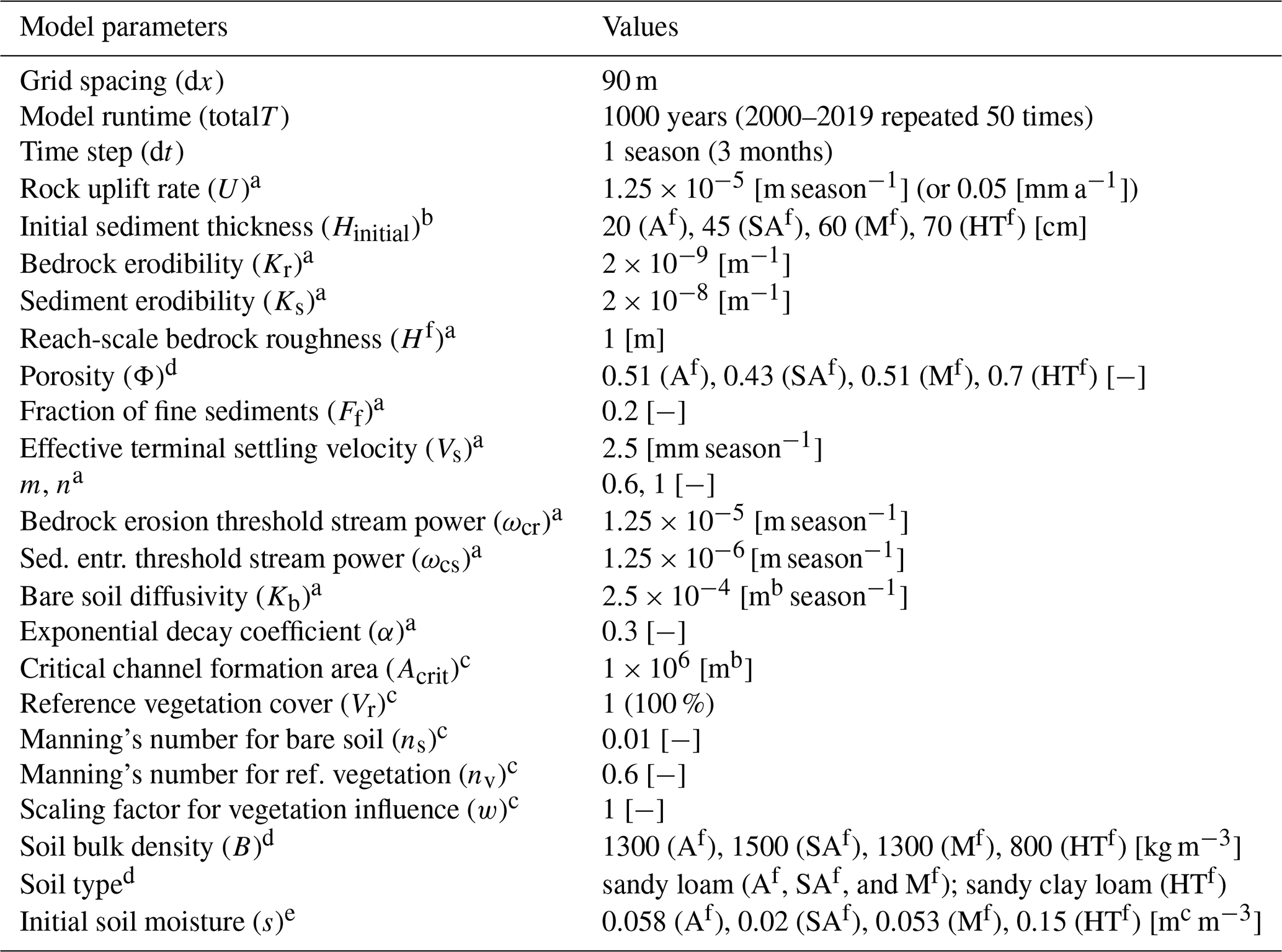
a Sharma et al. (2021), b Schaller et al. (2018), c Schmid et al. (2018), d Bernhard et al. (2018), e Übernickel et al. (2020). f A: arid; SA: semi-arid; M: Mediterranean; HT: humid–temperate setting.
The code and data used in this study are freely available via Zenodo (https://doi.org/10.5281/zenodo.8033782, Sharma and Ehlers, 2023).
The supplement related to this article is available online at: https://doi.org/10.5194/esurf-11-1161-2023-supplement.
HS and TAE designed the initial model setup and simulation programs. HS and TAE conducted model modifications, simulation runs, and analysis. HS prepared the initial paper draft, and both authors contributed to revisions.
The contact author has declared that neither of the authors has any competing interests.
Publisher's note: Copernicus Publications remains neutral with regard to jurisdictional claims made in the text, published maps, institutional affiliations, or any other geographical representation in this paper. While Copernicus Publications makes every effort to include appropriate place names, the final responsibility lies with the authors.
This article is part of the special issue “Earth surface shaping by biota (Esurf/BG/SOIL/ESD/ESSD inter-journal SI)”. It is not associated with a conference.
We acknowledge support from the Open Access Publishing Fund of the University of Tübingen. We would like to thank Erkan Istanbulluoglu, Omer Yetemen, and one anonymous reviewer for their constructive comments. We also thank Simon Mudd for editing this paper.
This research has been supported by the Deutsche Forschungs Gemeinschaft (grant nos. EH329/14-2, SPP-1803, and Research Training Group 1829 Integrated Hydrosystem Modelling).
This open-access publication was funded by the University of Tübingen.
This paper was edited by Simon Mudd and reviewed by Erkan Istanbulluoglu, Omer Yetemen, and one anonymous referee.
Avdeev, B., Niemi, N. A., and Clark, M. K.: Doing more with less: Bayesian estimation of erosion models with detrital thermochronometric data, Earth Planet. Sc. Lett., 305, 385–395, https://doi.org/10.1016/j.epsl.2011.03.020, 2011.
Beaudoing, H., Rodell, M., and NASA/GSFC/HSL: GLDAS Noah Land Surface Model L4 monthly 0.25 × 0.25 degree, Version 2.1, GES DISC [data set], https://doi.org/10.5067/SXAVCZFAQLNO, 2020.
Bernhard, N., Moskwa, L.-M., Schmidt, K., Oeser, R. A., Aburto, F., Bader, M. Y., Baumann, K., von Blanckenburg, F., Boy, J., van den Brink, L., Brucker, E., Büdel, B., Canessa, R., Dippold, M. A., Ehlers, T. A., Fuentes, J. P., Godoy, R., Jung, P., Karsten, U., Köster, M., Kuzyakov, Y., Leinweber, P., Neidhardt, H., Matus, F., Mueller, C. W., Oelmann, Y., Oses, R., Osses, P., Paulino, L., Samolov, E., Schaller, M., Schmid, M., Spielvogel, S., Spohn, M., Stock, S., Stroncik, N., Tielbörger, K., Übernickel, K., Scholten, T., Seguel, O., Wagner, D., and Kühn, P.: Pedogenic and microbial interrelations to regional climate and local topography: New insights from a climate gradient (arid to humid) along the Coastal Cordillera of Chile, Catena, 170, 335–355, https://doi.org/10.1016/j.catena.2018.06.018, 2018.
Bookhagen, B., Thiede, R. C., and Strecker, M. R.: Abnormal monsoon years and their control on erosion and sediment flux in the high, arid northwest Himalaya, Earth Planet. Sc. Lett., 231, 131–146, https://doi.org/10.1016/j.epsl.2004.11.014, 2005.
Brown, C. E.: Coefficient of Variation, in: Applied Multivariate Statistics in Geohydrology and Related Sciences, Springer, Berlin, Heidelberg, https://doi.org/10.1007/978-3-642-80328-4_13, 1998.
Buendia, C., Vericat, D., Batalla, R. J., and Gibbins, C. N.: Temporal Dynamics of Sediment Transport and Transient In-channel Storage in a Highly Erodible Catchment: Linking sediment sources, rainfall patterns and sediment yield, Land Degrad. Dev., 27, 1045–1063, https://doi.org/10.1002/ldr.2348, 2016.
Carretier, S., Tolorza, V., Regard, V., Aguilar, G., Bermúdez, M. A., Martinod, J., Guyot, J.-L., Hérail, G., and Riquelme, R.: Review of erosion dynamics along the major N-S climatic gradient in Chile and perspectives, Geomorphology, 300, 45–68, https://doi.org/10.1016/j.geomorph.2017.10.016, 2018.
Cerdà, A.: The influence of aspect and vegetation on seasonal changes in erosion under rainfall simulation on a clay soil in Spain, Can. J. Soil Sci., 78, 321–330, https://doi.org/10.4141/S97-060, 1998.
Chakrapani, G. J.: Factors controlling variations in river sediment loads, Curr. Sci., 88, 569–575, 2005.
Dal Bo, I., Klotzsche, A., Schaller, M., Ehlers, T. A., Kaufmann, M. S., Fuentes Espoz, J. P., Vereecken, H., and Van Der Kruk, J.: Geophysical imaging of regolith in landscapes along a climate and vegetation gradient in the Chilean coastal cordillera, Catena, 180, 146–159, https://doi.org/10.1016/j.catena.2019.04.023, 2019.
Deal, E., Favre, A. C., and Braun, J.: Rainfall variability in the Himalayan orogen and its relevance to erosion processes: Rainfall variability in the Himalayas, Water Resour. Res., 53, 4004–4021, https://doi.org/10.1002/2016WR020030, 2017.
Didan, K.: MOD13Q1 MODIS/Terra Vegetation Indices 16-Day L3 Global 250 m SIN Grid V006, USGS [data set], https://doi.org/10.5067/MODIS/MOD13Q1.006, 2015.
Earth Resources Observation And Science (EROS) Center: Shuttle Radar Topography Mission (SRTM) Void Filled, https://doi.org/10.5066/F7F76B1X, 2017.
Fernandes, N. F. and Dietrich, W. E.: Hillslope evolution by diffusive processes: The timescale for equilibrium adjustments, Water Resour. Res., 33, 1307–1318, https://doi.org/10.1029/97wr00534, 1997.
Ferreira, V. and Panagopoulos, T.: Seasonality of Soil Erosion Under Mediterranean Conditions at the Alqueva Dam Watershed, Environ. Manage., 54, 67–83, https://doi.org/10.1007/s00267-014-0281-3, 2014.
Gabarrón-Galeote, M. A., Martínez-Murillo, J. F., Quesada, M. A., and Ruiz-Sinoga, J. D.: Seasonal changes in the soil hydrological and erosive response depending on aspect, vegetation type and soil water repellency in different Mediterranean microenvironments, Solid Earth, 4, 497–509, https://doi.org/10.5194/se-4-497-2013, 2013.
Gao, P., Li, Z., and Yang, H.: Variable discharges control composite bank erosion in Zoige meandering rivers, Catena, 204, 105384, https://doi.org/10.1016/j.catena.2021.105384, 2021.
Garatuza-Payán, J., Sánchez-Andrés, R., Sánchez-Carrillo, S., and Navarro, J. M.: Using remote sensing to investigate erosion rate variability in a semiarid watershed, due to changes in vegetation cover, IAHS-AISH P., 292, 144–151, 2005.
Glodny, J., Gräfe, K., Echtler, H., and Rosenau, M.: Mesozoic to Quaternary continental margin dynamics in South-Central Chile (36–42∘ S): the apatite and zircon fission track perspective, Int. J. Earth Sci., 97, 1271–1291, https://doi.org/10.1007/s00531-007-0203-1, 2008.
Green, W. H. and Ampt, G. A.: Studies on Soil Phyics, J. Agr. Sci., 4, 1–24, https://doi.org/10.1017/S0021859600001441, 1911.
Hancock, G. and Lowry, J.: Hillslope erosion measurement – a simple approach to a complex process, Hydrol. Process., 29, 4809–4816, 2015.
Hancock, G. and Lowry, J.: Quantifying the influence of rainfall, vegetation and animals on soil erosion and hillslope connectivity in the monsoonal tropics of northern Australia, Earth Surf. Proc. Land., 46, 2110–2123, https://doi.org/10.1002/esp.5147, 2021.
Herrmann, S. M. and Mohr, K. I.: A Continental-Scale Classification of Rainfall Seasonality Regimes in Africa Based on Gridded Precipitation and Land Surface Temperature Products, J. Appl. Meteorol. Clim., 50, 2504–2513, https://doi.org/10.1175/JAMC-D-11-024.1, 2011.
Hobley, D. E. J., Adams, J. M., Nudurupati, S. S., Hutton, E. W. H., Gasparini, N. M., Istanbulluoglu, E., and Tucker, G. E.: Creative computing with Landlab: an open-source toolkit for building, coupling, and exploring two-dimensional numerical models of Earth-surface dynamics, Earth Surf. Dynam., 5, 21–46, https://doi.org/10.5194/esurf-5-21-2017, 2017.
Hou, J., Zhu, H., Fu, B., Lu, Y., and Zhou, J.: Functional traits explain seasonal variation effects of plant communities on soil erosion in semiarid grasslands in the Loess Plateau of China, Catena, 194, 104743, https://doi.org/10.1016/j.catena.2020.104743, 2020.
Howard, A. D.: A detachment-limited model of drainage basin evolution, Water Resour. Res., 30, 2261–2285, 1994.
Huang, S., Tang, L., Hupy, J. P., Wang, Y., and Shao, G.: A commentary review on the use of normalized difference vegetation index (NDVI) in the era of popular remote sensing, J. Forestry Res., 32, 1–6, https://doi.org/10.1007/s11676-020-01155-1, 2021.
Huete, A., Didan, K., Miura, T., Rodriguez, E. P., Gao, X., and Ferreira, L. G.: Overview of the radiometric and biophysical performance of the MODIS vegetation indices, Remote Sens. Environ., 83, 195–213, https://doi.org/10.1016/S0034-4257(02)00096-2, 2002.
Istanbulluoglu, E.: Vegetation-modulated landscape evolution: Effects of vegetation on landscape processes, drainage density, and topography, J. Geophys. Res., 110, F02012, https://doi.org/10.1029/2004jf000249, 2005.
Istanbulluoglu, E. and Bras, R. L.: On the dynamics of soil moisture, vegetation, and erosion: Implications of climate variability and change, Water Resour. Res., 42, W06418, https://doi.org/10.1029/2005WR004113, 2006.
Johnstone, S. A. and Hilley, G. E.: Lithologic control on the form of soil-mantled hillslopes, Geology, 43, 83–86, https://doi.org/10.1130/G36052.1, 2014.
Julien, P. Y., Saghafian, B., and Ogden, F. L.: Raster-based hydrologic modeling of spatially-varied surface runoff, J. Am. Water Resour. As., 31, 523–536, https://doi.org/10.1111/j.1752-1688.1995.tb04039.x, 1995.
Langbein, W. B. and Schumm, S. A.: Yield of sediment in relation to mean annual precipitation, EOS Trans. Am. Geophys. Union, 39, 1076–1084, https://doi.org/10.1029/TR039i006p01076, 1958.
Leyland, J., Hackney, C. R., Darby, S. E., Parsons, D. R., Best, J. L., Nicholas, A. P., Aalto, R., and Lague, D.: Extreme flood-driven fluvial bank erosion and sediment loads: direct process measurements using integrated Mobile Laser Scanning (MLS) and hydro-acoustic techniques: Direct measurement of flood-driven erosion using MLS and MBES, Earth Surf. Proc. Land., 42, 334–346, https://doi.org/10.1002/esp.4078, 2016.
Melnick, D.: Rise of the central Andean coast by earthquakes straddling the Moho, Nat. Geosci., 9, 401–407, https://doi.org/10.1038/ngeo2683, 2016.
Melnick, D., Bookhagen, B., Strecker, M. R., and Echtler, H. P.: Segmentation of megathrust rupture zones from fore-arc deformation patterns over hundreds to millions of years, Arauco peninsula, Chile: Earthquake segmentation at Arauco, J. Geophys. Res.-Sol. Ea., 114, B01407, https://doi.org/10.1029/2008JB005788, 2009.
Mosaffaie, J., Ekhtesasi, M. R., Dastorani, M. T., Azimzadeh, H. R., and Zare Chahuki, M. A.: Temporal and spatial variations of the water erosion rate, Arab. J. Geosci., 8, 5971–5979, https://doi.org/10.1007/s12517-014-1628-z, 2015.
Oeser, R. A., Stroncik, N., Moskwa, L.-M., Bernhard, N., Schaller, M., Canessa, R., Brink, L. van den, Köster, M., Brucker, E., Stock, S., Fuentes, J. P., Godoy, R., Matus, F. J., Pedraza, R. O., McIntyre, P. O., Paulino, L., Seguel, O., Bader, M. Y., Boy, J., Dippold, M. A., Ehlers, T. A., Kühn, P., Kuzyakov, Y., Leinweber, P., Scholten, T., Spielvogel, S., Spohn, M., Übernickel, K., Tielbörger, K., Wagner, D., and von Blanckenburg, F.: Chemistry and microbiology of the Critical Zone along a steep climate and vegetation gradient in the Chilean Coastal Cordillera, Catena, 170, 183–203, https://doi.org/10.1016/j.catena.2018.06.002, 2018.
Rengers, F. K., McGuire, L., Kean, J. W., Staley, D. M., and Hobley, D. E. J.: Model simulations of flood and debris flow timing in steep catchments after wildfire, Water Resour. Res., 52, 6041–6061, https://doi.org/10.1002/2015WR018176, 2016.
Rodell, M., Houser, P. R., Jambor, U., Gottschalck, J., Mitchell, K., Meng, C.-J., Arsenault, K., Cosgrove, B., Radakovich, J., Bosilovich, M., Entin, J. K., Walker, J. P., Lohmann, D., and Toll, D.: The Global Land Data Assimilation System, B. Am. Meteorol. Soc., 85, 381–394, https://doi.org/10.1175/BAMS-85-3-381, 2004.
Schaller, M. and Ehlers, T. A.: Comparison of soil production, chemical weathering, and physical erosion rates along a climate and ecological gradient (Chile) to global observations, Earth Surf. Dynam., 10, 131–150, https://doi.org/10.5194/esurf-10-131-2022, 2022.
Schaller, M., Ehlers, T. A., Lang, K. A. H., Schmid, M., and Fuentes-Espoz, J. P.: Addressing the contribution of climate and vegetation cover on hillslope denudation, Chilean Coastal Cordillera (26∘–38∘ S), Earth Planet. Sc. Lett., 489, 111–122, https://doi.org/10.1016/j.epsl.2018.02.026, 2018.
Schaller, M., Dal Bo, I., Ehlers, T. A., Klotzsche, A., Drews, R., Fuentes Espoz, J. P., and van der Kruk, J.: Comparison of regolith physical and chemical characteristics with geophysical data along a climate and ecological gradient, Chilean Coastal Cordillera (26 to 38∘ S), SOIL, 6, 629–647, https://doi.org/10.5194/soil-6-629-2020, 2020.
Schmid, M., Ehlers, T. A., Werner, C., Hickler, T., and Fuentes-Espoz, J.-P.: Effect of changing vegetation and precipitation on denudation – Part 2: Predicted landscape response to transient climate and vegetation cover over millennial to million-year timescales, Earth Surf. Dynam., 6, 859–881, https://doi.org/10.5194/esurf-6-859-2018, 2018.
Sharma, H. and Ehlers, T. A.: LandLab investigations into the seasonal effects of precipitation and vegetation change on catchment erosion, Zenodo [code and data set], https://doi.org/10.5281/zenodo.8033782, 2023.
Sharma, H., Ehlers, T. A., Glotzbach, C., Schmid, M., and Tielbörger, K.: Effect of rock uplift and Milankovitch timescale variations in precipitation and vegetation cover on catchment erosion rates, Earth Surf. Dynam., 9, 1045–1072, https://doi.org/10.5194/esurf-9-1045-2021, 2021.
Shobe, C. M., Tucker, G. E., and Barnhart, K. R.: The SPACE 1.0 model: a Landlab component for 2-D calculation of sediment transport, bedrock erosion, and landscape evolution, Geosci. Model Dev., 10, 4577–4604, https://doi.org/10.5194/gmd-10-4577-2017, 2017.
Starke, J., Ehlers, T. A., and Schaller, M.: Latitudinal effect of vegetation on erosion rates identified along western South America, Science, 367, 1358–1361, https://doi.org/10.1126/science.aaz0840, 2020.
Steegen, A., Govers, G., Nachtergaele, J., Takken, I., Beuselinck, L., and Poesen, J.: Sediment export by water from an agricultural catchment in the Loam Belt of central Belgium, Geomorphology, 33, 25–36, https://doi.org/10.1016/S0169-555X(99)00108-7, 2000.
Stephenson, J., Gallagher, K., and Holmes, C.: A Bayesian approach to calibrating apatite fission track annealing models for laboratory and geological timescales, Geochim. Cosmochim. Ac., 70, 5183–5200, https://doi.org/10.1016/j.gca.2006.07.027, 2006.
Suescún, D., Villegas, J. C., León, J. D., Flórez, C. P., García-Leoz, V., and Correa-Londoño, G. A.: Vegetation cover and rainfall seasonality impact nutrient loss via runoff and erosion in the Colombian Andes, Reg. Environ. Change, 17, 827–839, https://doi.org/10.1007/s10113-016-1071-7, 2017.
Tucker, G. E. and Bras, R. L.: A stochastic approach to modeling the role of rainfall variability in drainage basin evolution, Water Resour. Res., 36, 1953–1964, https://doi.org/10.1029/2000wr900065, 2000.
Tucker, G. E., Lancaster, S. T., Gasparini, N. M., and Bras, R. L.: Modeling floodplain dynamics and stratigraphy: implications for geoarchaeology, Final Technical Report (Part II-C), Contract Number DACA88-95-C-0017, USACERL – US Army Corps of Engineers Construction Engineering Research Laboratory, 16 pp., https://web.mit.edu/hydrology/Public/CHILDProject/floodplain.pdf (last access: 17 August 2022), 1999.
Übernickel, K., Ehlers, T. A., Ershadi, M. R., Paulino, L., Fuentes Espoz, J.-P., Maldonado, A., Oses-Pedraza, R., and von Blanckenburg, F.: Time series of meteorological station data in the EarthShape study areas of in the Coastal Cordillera, Chile, GFZ [data set], https://doi.org/10.5880/FIDGEO.2020.043, 2020.
Van Der Meer, F., Bakker, W., Scholte, K., Skidmore, A., De Jong, S., Clevers, J., Addink, E., and Epema, G.: Spatial scale variations in vegetation indices and above-ground biomass estimates: Implications for MERIS, Int. J. Remote Sens., 22, 3381–3396, https://doi.org/10.1080/01431160152609227, 2001.
Wang, L., Zheng, F., Liu, G., Zhang, X. J., Wilson, G. V., Shi, H., and Liu, X.: Seasonal changes of soil erosion and its spatial distribution on a long gentle hillslope in the Chinese Mollisol region, Int. Soil Water Conserv. Res., 9, 394–404, https://doi.org/10.1016/j.iswcr.2021.02.001, 2021.
Wei, W., Chen, L., Zhang, H., and Chen, J.: Effect of rainfall variation and landscape change on runoff and sediment yield from a loess hilly catchment in China, Environ. Earth Sci., 73, 1005–1016, https://doi.org/10.1007/s12665-014-3451-y, 2015.
Whipple, K. X. and Tucker, G. E.: Dynamics of the stream-power river incision model: Implications for height limits of mountain ranges, landscape response timescales, and research needs, J. Geophys. Res.-Sol. Ea., 104, 17661–17674, https://doi.org/10.1029/1999jb900120, 1999.
Wulf, H., Bookhagen, B., and Scherler, D.: Seasonal precipitation gradients and their impact on fluvial sediment flux in the Northwest Himalaya, Geomorphology, 118, 13–21, https://doi.org/10.1016/j.geomorph.2009.12.003, 2010.
Yetemen, O., Istanbulluoglu, E., Flores-Cervantes, J. H., Vivoni, E. R., and Bras, R. L.: Ecohydrologic role of solar radiation on landscape evolution, Water Resour. Res., 51, 1127–1157, https://doi.org/10.1002/2014wr016169, 2015.
Zhang, S., Li, Z., Hou, X., and Yi, Y.: Impacts on watershed-scale runoff and sediment yield resulting from synergetic changes in climate and vegetation, Catena, 179, 129–138, https://doi.org/10.1016/j.catena.2019.04.007, 2019.
Zhang, W., An, S., Xu, Z., Cui, J., and Xu, Q.: The impact of vegetation and soil on runoff regulation in headwater streams on the east Qinghai–Tibet Plateau, China, Catena, 87, 182–189, https://doi.org/10.1016/j.catena.2011.05.020, 2011.
Zhang, X., Yu, G. Q., Li, Z. B., and Li, P.: Experimental Study on Slope Runoff, Erosion and Sediment under Different Vegetation Types, Water Resour. Manag., 28, 2415–2433, https://doi.org/10.1007/s11269-014-0603-5, 2014.
Zheng, F. L.: Effect of Vegetation Changes on Soil Erosion on the Loess Plateau, Pedosphere, 16, 420–427, https://doi.org/10.1016/S1002-0160(06)60071-4, 2006.
Ziese, M., Rauthe-Schöch, A., Becker, A., Finger, P., Rustemeier, E., and Schneider, U.: GPCC Full Data Daily Version 2020 at 1.0∘: Daily Land-Surface Precipitation from Rain-Gauges built on GTS-based and Historic Data: Gridded Daily Totals (2020), DWD [data set], https://doi.org/10.5676/DWD_GPCC/FD_D_V2020_100, 2020.