the Creative Commons Attribution 4.0 License.
the Creative Commons Attribution 4.0 License.
 | 13 Mar 2023
Modeling the inhibition effect of straw checkerboard barriers on wind-blown sand
Straw checkerboard barriers (SCBs) are usually laid to prevent or delay desertification caused by eolian sand erosion in arid and semiarid regions. Understanding the impact of SCBs and their laying length on eolian sand erosion is of great significance to reduce damage and laying costs. In this study, a three-dimensional wind-blown-sand model in the presence of SCBs was established by introducing the splash process and equivalent sand barriers into a large-eddy simulation airflow. From this model, the inhibition effect of SCBs on wind-blown sand was studied qualitatively, and the sensitivity of eolian sand erosion to the laying length was investigated. The results showed that the decrease in the wind speed in the SCB area oscillates along the flow direction. Moreover, the longer the laying lengths are, the lower the wind speed and the sand transport rate in the stable stage behind SCBs will be. We further found that the concentration of sand particles near the side of SCBs is higher than that in its central region, which is qualitatively consistent with previous research. Our results also indicated that whether the wind speed will decrease below the impact threshold or the fluid threshold is the key factor affecting whether sand particles can penetrate the SCBs and form stable wind-blown sand behind the SCBs under the same conditions. Although our model does not include the collision between sand particles and SCB walls, which makes the suppression of wind-blown sand by SCBs obtained from the current model conservative, our research still provides theoretical support for the minimum laying length of SCBs in anti-desertification projects.
- Article
(14368 KB) - Full-text XML
-
Supplement
(5805 KB) - BibTeX
- EndNote


In arid and semiarid areas, eolian sand erosion is becoming increasingly serious. Preventing or delaying the process of desertification is a major challenge worldwide, especially in the transitional areas between deserts and oases. At present, shelterbelts (Wang et al., 2010), sand fences (Bitog et al., 2009; Hatanaka and Hotta, 1997; Li and Sherman, 2015; Lima et al., 2017; Wilson, 2004), windbreak walls (Bouvet et al., 2006; Santiago et al., 2007), hole plate-type sand barriers (Chen et al., 2019) and straw checkerboard sand barriers (Bo et al., 2015; Huang et al., 2013; Wang and Zheng, 2002; Xu et al., 2018) are the main structures used to prevent desertification. Among these structures, straw checkerboard barriers (SCBs) are the most commonly used in anti-desertification projects because of their advantages of being easy to obtain and relatively low cost (Zheng, 2009). Laying SCBs could play an important role in the ecological restoration of sandy land ecosystems (Zhang et al., 2018) and vegetation restoration. Some research has shown that SCBs can effectively reduce the surface wind speed (Qu et al., 2007), increase the surface roughness (Zhang et al., 2016), weaken the sand transport rate (Bo et al., 2015), and change the distribution of eolian sandy soil particles and soil organic carbon (Dai et al., 2019), thus protecting the survival of vegetation and achieving sustainable development of oases and ecological environments.
In recent decades, SCBs have been widely used in northwestern China, which is seriously damaged by eolian sand erosion. For example, SCBs have been laid on the sides of roadbeds along railways such as the Baotou–Lanzhou Railway, Wuda–Jilantai Railway (Wang, 1996), Gantang–Wuwei Railway (Yang, 1995), Lanzhou–Xinjiang Railway (Binwen et al., 1998; Li et al., 1998; Cheng et al., 2016) and Qinghai–Tibet Railway (Cheng and Xue, 2014; Zhang et al., 2010), as well as in windy sand areas beside desert roads such as the Taklamakan Desert Highway (Li et al., 2006; Qu et al., 2007), Tarim Desert Highway (Xu et al., 1998) and Minqin Desert Highway. In addition, SCBs are adopted by some countries that are also affected by eolian sand erosion, such as Ghana, Egypt and Iran (Zheng, 2009). Although SCBs have been widely used, their design size and laying methods are mainly determined by practical experience or repeated tests. For example, for the sand fence, which has a similar effect to the SCB, Li and Sherman (2015) combined experimental and field data to conclude that the optimal design of a sand fence is closely related to its aerodynamics and morphodynamics. The effect of sand fences with different porosities, spacings and heights on the wind field is significant (Lima et al., 2017, 2020). However, the complexity of the flow field around the SCBs and the movement of sand particles, as well as the coupling of particles and flow field, make this problem more difficult. Therefore, it is necessary to study the characteristics of turbulence inside and behind the SCBs and the influence mechanism of the laying length on wind speed and erosion.
Wang and Zheng (2002) proposed an ideal single-row uniformly distributed vortex model to simplify the flow field of wind-blown sand. Based on their model, the corresponding relationship between the side length and the height of a single SCB was analyzed. Their theoretical results are similar to the size of the SCBs laid in the Tarim Desert Highway (1 m in side length and 15–20 cm in height). Qiu et al. (2004) noted that since the concentration of wind-blown sand below 10 cm near the surface is relatively high, the height of the SCBs should be designed to be 10–20 cm to effectively prevent eolian sand erosion. The experimental results of Zhang et al. (2018) indicated that the SCB has the best protective effect when its side length is 1 m. These works are of great help to the design of a single SCB. Based on these empirical sizes of the SCBs, researchers have tried to analyze the effect of SCBs on the flow field and particles from the perspective of turbulence. Huang et al. (2013) used a two-dimensional large-eddy simulation and discrete particle tracking methods to simulate wind-blown-sand movement inside simplified two-dimensional SCBs. The effect of SCBs on surface wind speed was analyzed. They found that sand particles could be aggregated at the inner walls of the SCBs due to the influence of the vortex or the backflow. Then, a V-shaped sand trough was formed, which is similar to the actual situation. Bo et al. (2015) equated the SCBs to the source term of the standard k–ε turbulence model and analyzed the influence of SCBs on the wind speed profile in a two-dimensional flow field without sand particles. They divided the streamwise velocity profile in a flow field containing SCBs into approximately three different log-linear functions and obtained the relationship between them and friction wind speeds. Although these two-dimensional models can reflect the effect of the SCBs on the flow field to some extent, they are far from the real turbulence. Moreover, since the three-dimensional SCB is simplified into a two-dimensional plane with only the streamwise direction and vertical direction, the impact of this simplification is uncertain. For this reason, Xu et al. (2018) simulated wind-blown-sand movement on the SCB surface under a three-dimensional flow field using OpenFOAM and mainly analyzed the influence of the flow field inside the SCBs on the movement of sand particles. They concluded that the wind vortex is the main cause of the internal morphology of the straw checkerboard. They found that the vortex drives particles inside the SCBs towards the front and sidewalls, making the erosional form in SCB cells low in the middle and high near all sides. However, the SCBs are completely equivalent to the solid as the bottom boundary condition in their model. As a non-solid material, SCBs can be penetrated by wind in practice. It only weakens the wind speed and is thus not equivalent to a solid. For example, Dupont et al. (2014) equated surface vegetation to a resistance force through the resistance coefficient and leaf area coefficient, meaning that the wind will be resisted as it passes through these equivalent regions.
To reasonably introduce the SCBs and consider their coupling with turbulence, SCBs and the surface splash process, the development of a three-dimensional model is needed. In this paper, a three-dimensional numerical coupled model of wind-blown sand in the presence of SCBs was carried out to study the inhibition effect of the laying length on eolian sand erosion. The large-eddy simulation approach was used to simulate clean airflow with the saltation process. Furthermore, we added a volume drag force into the Navier–Stokes equations by using the drag source method to realize the coupling between the SCBs and the wind-blown-sand movement. Sections 2 and 3 present the three-dimensional numerical coupled model and its validation, respectively. In Sect. 4, the effects of the SCB laying length on clean airflow and sand-laden flow under different friction wind speeds are studied. Finally, Sect. 5 summarizes the main conclusions.
The Advanced Regional Prediction System (ARPS) has been widely used to simulate turbulent boundary layer particle-laden flow, such as wind-blown sand (Dupont et al., 2013; Huang, 2020) and wind-blown snow (Huang and Wang, 2016; Li et al., 2018). The standard version of the program is described in the ARPS user's manual (Xue et al., 1995), and its validation cases are referred to Xue et al. (2000, 2001). For this study, some suitable models were added to simulate turbulent boundary-layer flow in the presence of SCBs with saltating sand particles. A detailed description of these modifications is shown in the following subsections.
2.1 Turbulent boundary layer flow
The basic flow fields in our numerical simulation are established based on ARPS (version 5.3.4). The filtered continuity and momentum equations, including the viscous drag force terms of sand particles as well as SCBs, are shown as follows (Dupont et al., 2013; Vinkovic et al., 2006):
where i=1, 2, and 3 correspond to the streamwise, spanwise, and wall-normal directions (i.e., x1=x, x2=y, x3=z, u1=u, u2=v, u3=w), respectively; , , and represent the filtered wind speed, pressure, and potential temperature, respectively; ν is a damping coefficient of the attenuate acoustic waves; ρf is the air density; g is the acceleration of gravity; is the main feedback force, including the feedback force provided by sand particles (, as shown in Sect. 2.2) and the SCBs (, as shown in Sect. 2.5); δij=1 if i=j, otherwise δij=0; are the SGS (sub-grid-scale) stresses (Smagorinsky, 1963); and cp and cv are the specific heat of air at constant pressure and volume, respectively.
To solve the above equations, the SGS stresses can be closed as follows:
where Δ is the grid scale and Csgs depends on the Germano SGS closure method (Germano et al., 1991).
For the governing equations mentioned above, periodic boundary conditions are applied for the spanwise direction. The upper and lower boundaries are set as a stress-free condition and a rigid ground condition, respectively. The outlet boundary is used as an open radiation condition in this paper. The inlet boundary is a given logarithmic profile:
Here k=0.41 is von Kármán constant, is the aerodynamic surface roughness (Kok et al., 2012), dmean is the mean diameter of the sand particles and u* is the friction speed of inflow. Additionally, the simulation is driven by a constant flow corresponding to the given logarithmic wind profile. To accelerate the development of boundary layer flow, a modified Spalart method (Lund et al., 1998) is applied to the inlet condition and the recycling plane at % (Inoue and Pullin, 2011). xref=5 m is the position of the recycling plane, and Lx=40 m is the total length of the flow direction. The specific method reassigns the calculated mean velocity and fluctuation at the recycling plane to the inlet at each fluid time step. A similar application is described by Xu et al. (2018).
2.2 Movement of the sand particles
Saltating particles are moved by the drag force, gravity, electric field force, Magnus force, Saffman force and so on (Murphy and Hooshiari, 1982). In our model, the drag force and gravity are considered, ignoring other minor factors (Kok et al., 2012; Zou et al., 2007). We employ the Lagrangian point-particle method to describe particle motions, and the equations of particles with different sizes in three directions can be expressed as
where mp is the mass of sand particles and is the drag coefficient of sand particles (Cheng, 1997). The particle Reynolds number can be expressed as
ρp and ρf are the density of sand particles and air, respectively; D is the diameter of sand particles; is the bulk fraction, which is the total sand volumes within grid to the bulk of unit grid; ΔV is the bulk of unit grid; μ is the kinetic viscosity coefficient of air; and , , , , , and are the normal and tangential force of contact in three directions.
2.3 Particle collision
Modeling the collision process in the air among the ejection particles has been the focus of previous studies (Carneiro et al., 2013; Huang et al., 2007). In this paper, the “spring-damping model” is used to calculate the contact force when particles collide in the air. The contact force can be described as follows (Huang et al., 2017).
The normal force of contact is
where is the normal stiffness coefficient, ζ is the amount of overlap between particles during contact, Ri and Rj are the radius of particle i and j, rij is distance vector between particles, and vn,ij is the normal relative velocity vector. The normal damping coefficient can be expressed as
where mi and mj are the mass of particle i and j and ε=0.7 is restitution coefficient.
The tangential force of contact is
where is the tangential stiffness coefficient, ζt,ij is the tangential displacement and vt,ij is the tangential relative velocity vector. The tangential damping coefficient can be expressed as
2.4 Splash process
Splash processes not only serve as an indispensable part of the near-surface particle motions but also relate to the accuracy of emissions during upwards particle transport. There are a large number of collisions between particles and the ground. Meanwhile, other particles will be blown upwards when particles hit the ground, which is referred to as the splash process. If energy-based collision analysis is performed on a single particle, considerable time will be consumed. Therefore, researchers have parameterized some key variables in accordance with the characteristics of splashing, thereby simplifying the problem. We assume that there are enough sand and dust particles on the ground to splash when the particles impact the surface. If the particle collides with the bed, we assume the rebound probability as
where vimp is the impact speed and λ is an empirical parameter on the order of 2 s m−1 according to the previous study (Anderson et al., 1991). The rebound sand speed is 0.55 times the impact sand speed, and the rebound angle θreb is 40∘ (Zhou et al., 2006). Of course, at a certain speed, some new sand particles will be splashed. The ejection number is
where n0=0.4, A=0.68, B=0.39, ζ=5, C=0.92 and D=1.39 (Huang et al., 2017). θimp is the impact angle, μimp is the ratio of impact grain size to the mean size of the bed and dmean is the mean diameter of the sand particles. The ejection angle distributes randomly between 50 and 60∘ (Rice et al., 1995). The probability density distribution of the initial lifting speed follows
where is the ejection speed and the overbar represents a mean value (Anderson et al., 1991; Werner, 1990). The mean ejection speed can be expressed as (Kok and Renno, 2009)
Moreover, the sand particles satisfy the periodic boundary condition in the streamwise and spanwise directions. Following the idea of Dupont et al. (2013), aerodynamic entrainment is not considered in our model. A total of 10 000 initial particles are randomly released in the flow field (Huang, 2020), and the release height should be lower than 0.3 m (Shao and Raupach, 1992). The results of Dupont et al. (2013) showed that the number of released particles does not affect the final results but only the speed of wind-blown-sand development.
2.5 Parameters and the equivalent method of SCBs
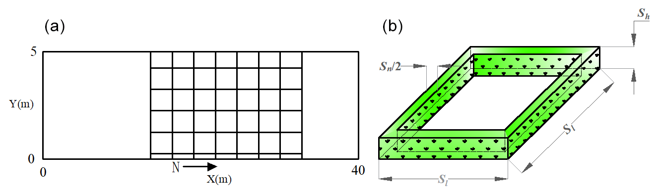
According to the experience of laying SCBs in practical engineering (Chang et al., 2000) and the theoretical results of Wang and Zheng (2002), in this paper the height of the SCB (Sh) is set to 10 cm, the side length of a single SCB (Sl) is set to 100 cm and the side thickness of the SCB (Sn) is set to 10 cm. The diagram of a single SCB is shown in Fig. 1b. Moreover, to study the inhibition effect of the laying length of SCBs (represented by N) on eolian sand erosion, we set N=5–10, 5–20 and 5–30 m in the simulation cases. The diagram of the laying SCBs is shown in Fig. 1a, and the main parameters of the SCBs are listed in Table 1.

The SCBs are equivalent to a volume resistance force through the resistance coefficient and leaf area coefficient; that is, the flow in these regions will be subject to an additional resistance force, which can be expressed as
where Cd is the drag coefficient, ad is the leaf area coefficient and U is the inflow wind speed. In the simulation, the value of Cd is 0.2 according to the parameters of Dupont et al. (2013). Nepf (2012) concluded that when the diameter of vegetation is 4–9 cm, the value of the leaf area coefficient a can reach 20 m−1. Therefore, according to the side thickness of the SCB presented in this paper, the leaf area coefficient is set as 40 m−1. Due to the limitation of the drag force method, the SCBs only affect the velocity of the flow field rather than the real presence. The current model considers the inhibition effect of the flow field on the particles and does not simulate the collision process between the sand particles and the SCBs. Therefore, this collision–obstruction process can be approximately simplified as the sudden drop in the drag force as the saltating particles pass through the region of the SCBs. The consequences of such a simplification may lead to an underestimation of the inhibition effect of the SCBs. Therefore, this limitation of the current model needs to be noted.
2.6 Calculation parameters
Wind tunnel experiments conducted by Shao and Raupach (1992) indicated that a complete “overshoot” was more than 10 m in the streamwise direction (Huang et al., 2014; Ma and Zheng, 2011). In Fig. 2, the computational domains are Lx=40 m, Ly=5 m and Lz=2 m in the streamwise, spanwise and wall-normal directions, respectively. Field experiments conducted by Baas and Sherman (2005) showed that the mean lateral size of sand streamers is approximately 0.2 m. To capture this structure, the mesh spacing is Nx=0.1 m and Ny=0.05 m in the streamwise and spanwise directions, respectively. In addition, in the near-wall region, logarithmic stretching has been adopted to ensure precision. The mean and minimum mesh spacing in the vertical direction is Nz=0.025 m and m, respectively. Therefore, the grids of the streamwise, spanwise and vertical directions are , respectively. The sand particle diameter satisfies the normal distribution: the mean diameter equals 200 µm, and the variance is ln (1.2). We first simulate the clean-air field flow in the presence of SCBs for 30 s to obtain the full development of the flow field. Then, we add sand particles to the flow field to obtain a sand-laden flow. After the wind-blown-sand flow becomes saturated, the simulations continue for another 20 s to perform the statistics. The fluid time step is Δts=0.0002 s, and the particle time step is Δtp=0.00005 s. The sand grain density is 2650 kg m−3, and the air density is 1.225 kg m−3. The main calculation parameters are listed in Table 2.

Figure 3(a) The spatial variation in the streamwise sand transport rate in the sand-laden flow. (b) The streamwise sand transport rate density with the height at the three flow direction positions.
3.1 Particle field validation
In Sect. 3.1, we will verify the validity of the model from the following two aspects. The sand transport rate is an important physical quantity in wind-blown sand, which is the embodiment of the sediment carrying capacity of the flow field (Zheng, 2009). Therefore, without considering the SCBs, we first compare the spatial variation in the sand transport rate in the sand-laden flow with the experimental results of Shao and Raupach (1992). The sand transport rate is calculated according to the following formula:
where represents the sand mass and Δx is the grid size in the flow direction. Whether the wind-blown-sand flow is saturated depends on the change in sediment transport at a certain streamwise position. The condition for judging saturation is given by Ma and Zheng (2011). The wind tunnel experimental results of Shao and Raupach (1992) showed that the streamwise sand transport rate first increased and then decreased until it was stable, which is called the overshoot phenomenon (Anderson and Haff, 1991; McEwan and Willetts, 1991). Figure 3a shows the comparison between the simulation results of the sand transport rate along the flow direction and the experimental results of Shao and Raupach (1992) under the same friction wind speed. As shown in Fig. 3a, our simulation results also show this phenomenon. However, unlike the other numerical simulation results (Huang et al., 2014; Ma and Zheng, 2011), our sediment transport rate results have an obvious fluctuation characteristic and are not smooth curves, which may be caused by the turbulence intermittency unique to the three-dimensional wind-blown-sand model. Moreover, we give the distribution results of the streamwise sand transport rate density with the height at the three flow direction positions, which are compared with the experimental results. From Fig. 3b, we can see that the distribution of the streamwise sand transport rate density with height follows the trend of exponential decline, and the sand transport rate density at x=6 m is significantly higher than that at x=1 m and x=14.5 m, which is consistent with the experimental results of Shao and Raupach (1992). This is because the streamwise position of x=6 m is in the peak region of the overshoot phenomenon, while the streamwise positions of x=1 m and x=14.5 m are in the rising region and stable region, respectively. Due to the massive accumulation of sand particles near the surface (0–20 mm), the concentrations cannot be easily measured. In Fig. 3b, our simulation results also show that the distribution of the streamwise sand transport rate density with heights below 10 mm still satisfies the trend of exponential decline. However, at a height of 2–3 mm, there is a slight change in this trend; that is, the rate of increase in the sand transport rate density slows down, which is not revealed in the experimental results. Due to the limitations of the large-eddy simulation, the simulation results near the wall may be distorted and require further experimental verification.
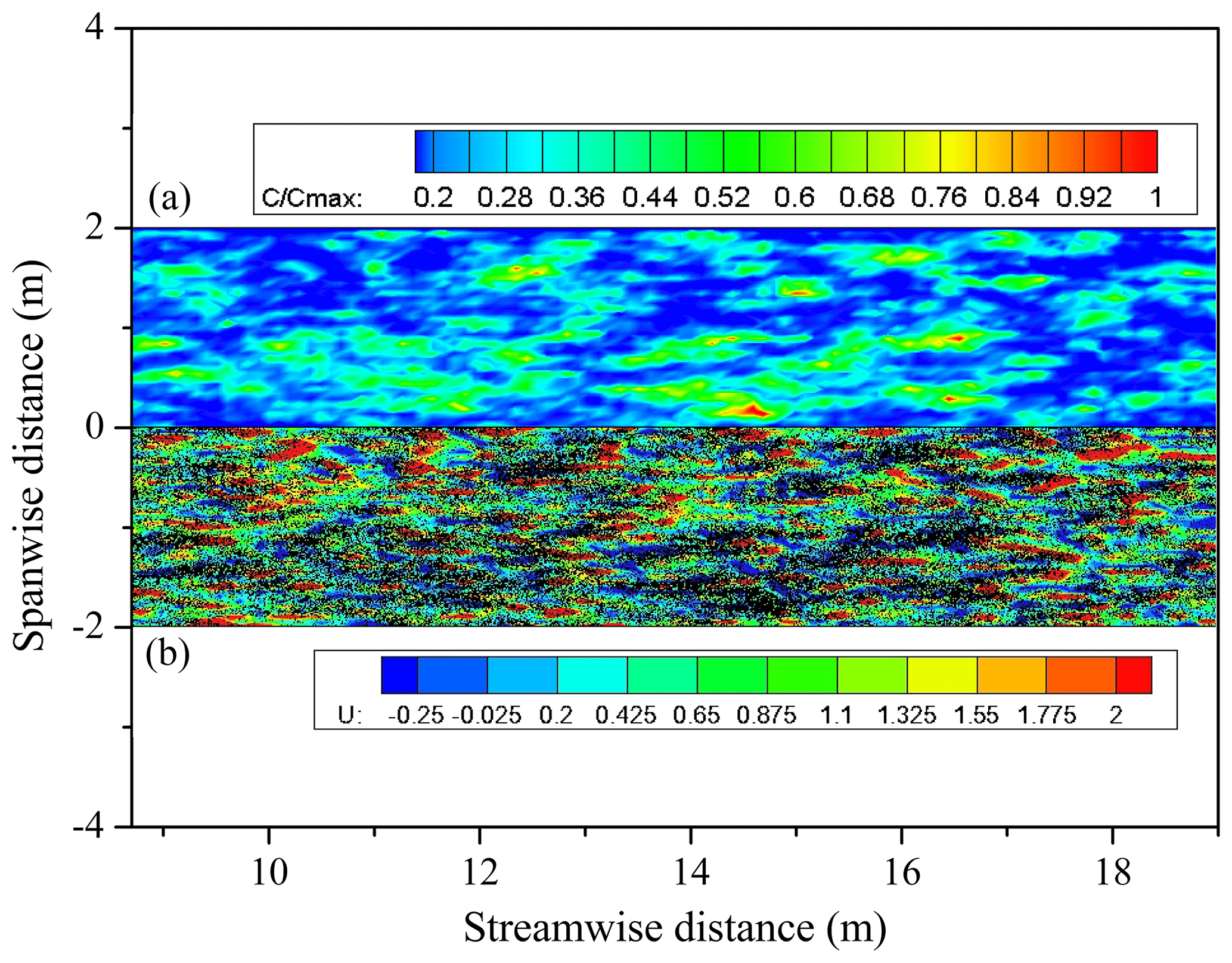
Figure 4(a) The top view of the sand streamer concentrations, where C represents the particle concentrations, Cmax represents the maximum particle concentrations. (b) The top view of the whole-particle positions and the streamwise velocity diagram of flow field with the height of 0.005 m, where the y coordinates are correspondingly shifted down by 2, the black dots represent the sand particles and U represents the streamwise wind speed of the sand-laden flow (uτ=0.3 m s−1).
Sand streamers, as a natural phenomenon in wind-blown sand, have been widely studied. Therefore, without considering the SCBs, we analyze the morphology of the sand streamer and its relationship with the flow field. In the meantime, the airborne particle concentration within a certain area can be calculated as
Figure 4a shows the top view of the particle-aggregation morphology in the stable stage of sand-laden flow. It can be seen from Fig. 4a that the concentration of sand particles is intermittent in both streamwise and spanwise directions. Moreover, we can see clearly that the morphological characteristics of the sand streamer are consistent with the observations of Baas and Sherman (2005), i.e., up to a few meters in the streamwise direction and approximately 0.2 m in the spanwise direction. Our model can sufficiently reproduce the “sand streamer” phenomenon in wind-blown sand. Here, we need to point out that the intermittence of turbulence complicates particle movement, especially when multiple streamers are connected end to end and the concentration is sufficiently close, meaning that super sand streamers up to tens of meters long will exist. Whether they are examining sand-laden flow or other two-phase flows, researchers are generally concerned about the aggregation of particles. We plot the position of particles and the streamwise velocity of the flow field in Fig. 4b and find that most particles are assembled in the low-speed streaks, which is consistent with the conclusion of the other particle-laden-flow studies (Lee and Lee, 2015; Richter, 2015).
3.2 Velocity field validation
The verification of the flow field part of the program is covered in detail in our previous works (Huang, 2020). In Sect. 3.2, we focus on the flow field verification after considering the SCBs. We verify the difference in the velocity profile and the surface roughness in the clean airflow with and without the SCBs. In previous work, the wind speed and surface roughness near the SCBs were both well studied (Dong et al., 2000; Qu et al., 2007; Wang et al., 1999). These works all pointed out that laying the SCBs can effectively increase the surface roughness and reduce the wind speed near the surface to play a role in inhibiting the wind-blown sand and fixing the sand particles. Figure 5a and b are the tangent plane (x–z plane) of the streamwise wind velocity without and with the SCBs, respectively. It can be seen intuitively that the existence of the SCBs significantly reduces the surface wind speed and increases the boundary layer thickness of the flow field. To reveal the difference quantitatively, we plot the wind speed profiles of different streamwise positions in the clean airflow containing the SCBs in Fig. 6a. The selected positions are x=1, 2, and 3 m in front of the SCBs; x=7.5, 12.5, and 17.5 m in the area containing the SCBs; and x=30, 35, and 39 m behind the SCBs. We can see that the wind speed profiles at the three positions in front of the SCBs are basically the same. In the area containing the SCBs, the existence of the SCBs reduces the surface wind speed and increases the thickness of the boundary layer (equivalent to increasing the surface roughness), as well as increases the incoming wind speed outside the boundary layer. Moreover, the longer the SCBs are, the thicker the boundary layer becomes, and the incoming wind speed outside the boundary layer will also increase. The flow field behind the SCBs may be complicated by the influence of the attached vortex generated by the SCBs, but the overall trend is the same, and the boundary layer thickness remains consistent. These results are qualitatively consistent with the conclusions of previous work (Dong et al., 2000; Qu et al., 2007; Wang et al., 1999), indicating that our model has effectively introduced the SCB module.
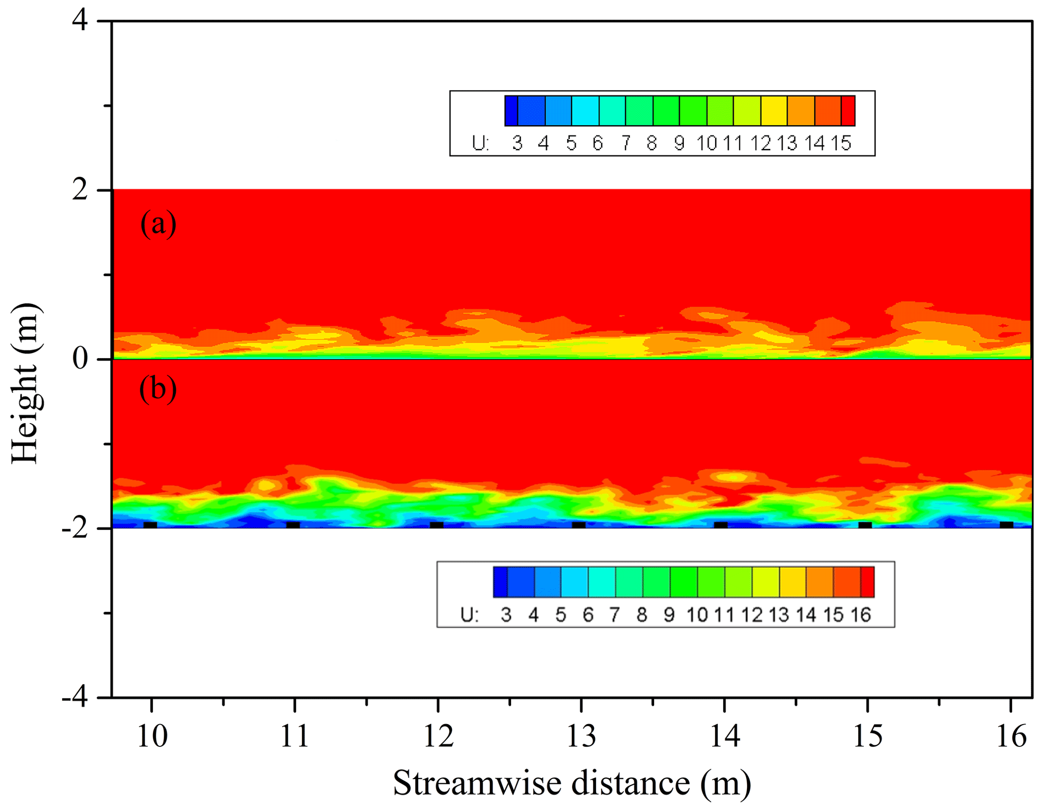
Figure 5The side view of x–z-plane streamwise velocity before (a) and after (b) containing the SCBs (uτ=0.6 m s−1; N=5–20 m; y=0 m). The y coordinates are correspondingly shifted down by 2 m in (b).
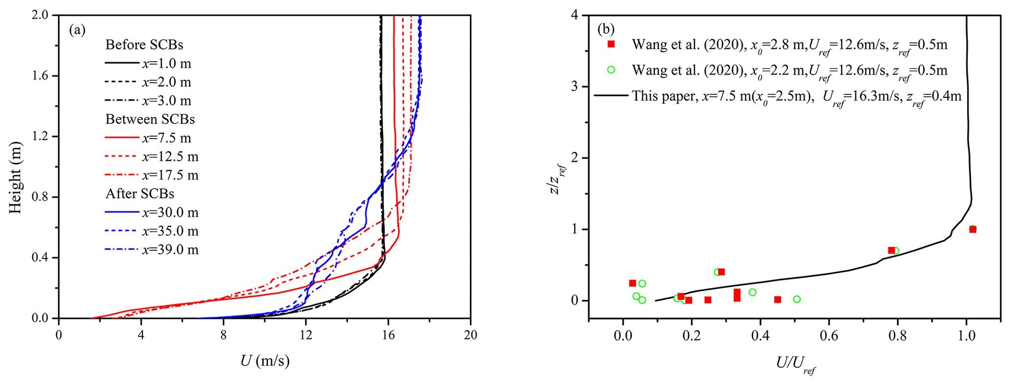
Figure 6(a) The wind speed profiles of different streamwise positions in the clean airflow containing the SCBs (uτ=0.6 m s−1; N=5–20 m). (b) The dimensionless wind speed varying with dimensionless height shown as a comparison between our simulated results and the existing experiment.
In addition, we compared the wind speed profiles with the experimental results of Wang et al. (2020). In Fig. 6b, the streamwise wind speed in the horizontal coordinate is dimensionless with the reference wind speed Uref, and the height in the vertical coordinate is dimensionless with the reference height zref. In the wind tunnel experiment conducted by Wang et al. (2020), the maximum boundary layer thickness is given as 0.5 m, so the reference height is taken as zref=0.5 m. Then, the wind speed at z=0.5 m is determined as the reference wind speed Uref=12.58 m s−1 based on the inlet wind profiles. In our simulation case, zref=0.4 m is the initial inlet boundary layer thickness, and Uref=16.3 m s−1 is the reference wind speed. We select the experimental results of wind speed profiles at the SCB belt positions x0=2.2 and 2.8 m along the flow direction to compare with our numerical results at x0=2.5 m (streamwise position x=7.5 m). The dimensionless results show that our results are consistent with the experimental results in quantitative and qualitative, which indicates that our model can reveal the inhibition effect of SCBs well on the flow field. In the following section, we will reveal more about the influence of the laying length on the wind field and its inhibition effect on wind-blown sand.
4.1 Influence of the SCBs on the clean airflow
Figure 7a and b show that the presence of the SCBs destroys the original streaks of the clean airflow and decreases the wind speed. In most cases, the wind speed in the central area of a single SCB is significantly higher than that in the surrounding area, showing a block of velocity distribution characteristics. Although the wind speed behind the SCBs will recover rapidly, there is a significant difference between the newly formed streaks and the original streaks of the flow field; that is, the streamwise scale of the streaks behind the SCBs is significantly shorter than before. The variation in streamwise wind speed at the different laying length cases (N=5–10, 5–20, 5–30 m) under the same friction wind speed (uτ=0.6 m s−1) is plotted in Fig. 8, where Fig. 8a corresponds to the wind speed at a height of 0.1 m, and Fig. 8b corresponds to the wind speed at a height of 0.2 m. Figure 8 shows an oscillating decrease in wind speed in the SCBs. In addition, behind the SCBs, the wind speed gradually increases and then stabilizes. The trend of wind speed reduction in the SCBs is consistent with the existing experimental results (Xu et al., 1982). The difference is that the reduction process of the wind speed around the SCBs exhibited an oscillatory attenuation instead of a continuous decrease, which was not revealed in the previous simulation results (Bo et al., 2015). Moreover, when the incoming wind speed is stable, the longer the laying lengths are, the lower the wind speed in the stable stage behind the SCBs will be. This is very useful information. On this basis, we can obtain the relationship between the laying length of the SCBs and the wind speed in the stable stage according to an actual situation. For example, the wind speed in the stable stage can be reduced to the impact threshold or the aerodynamic threshold on both sides of the desert highway to determine the minimum laying length of the SCBs and save laying costs. This is a potential application of our model and needs further experimental verification.

Figure 7The top view of x–y-plane streamwise velocity without (a) and with (b) the SCBs (z=0.005 m; uτ=0.6 m s−1; N=5–20 m).
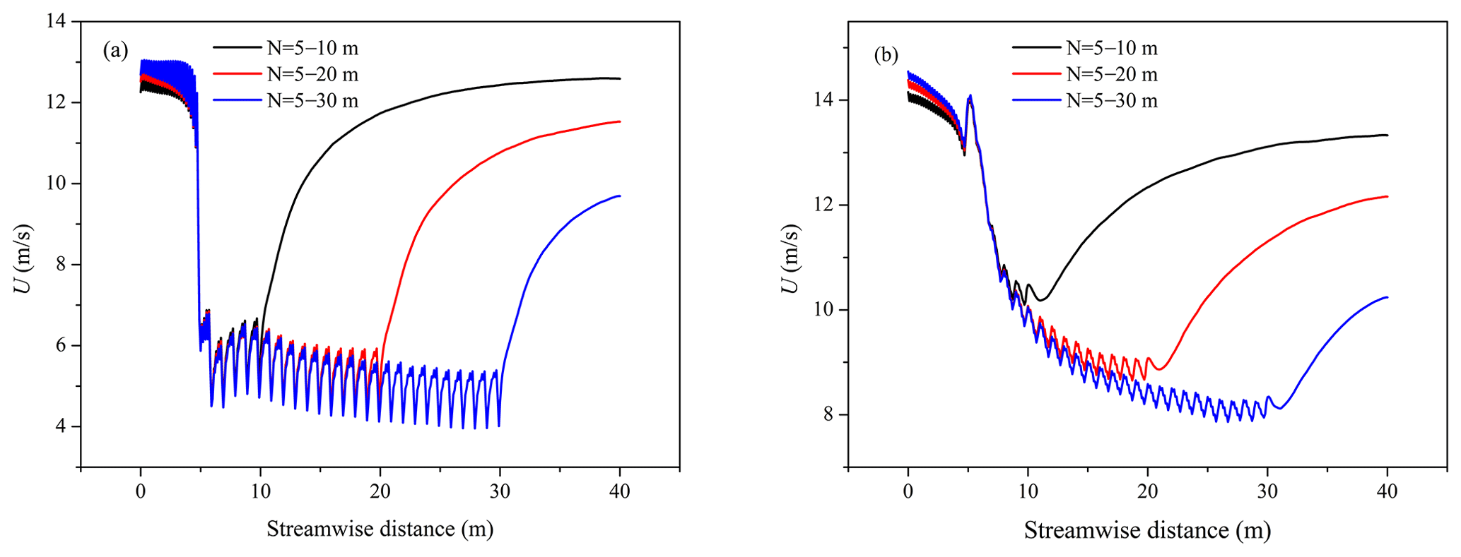
Figure 8The streamwise wind speed in the clean airflow containing the SCBs at a height of 0.1 m (a) and a height of 0.2 m (b) (uτ=0.6 m s−1; N=5–10, 5–20, 5–30 m).
4.2 Effect of sand particles on the flow field and its aggregation location
Sand particles were added to the clean-airflow field in the presence of SCBs to fully develop and reach stability. The top view of the particle positions of the wind-blown sand after reaching a stable state is shown in Fig. 9. From Fig. 9, we can see that when the wind-blown sand passes through the SCBs, the particle number obviously decreases gradually, and the inhibition effect of the SCBs on the wind-blown sand can be visualized. Moreover, the motion of sand particles behind the SCBs returns to complete wind-blown-sand movement. We then plot the sand concentrations of the region in the presence of SCBs in Fig. 10. Combining the laying position of the SCBs, as well as the corresponding sand concentrations, we can clearly see that the concentration of sand particles near the side of the SCBs is higher than that in its central region, which is consistent with the conclusion of Xu et al. (2018). On the one hand, the wind speed near the side of SCBs is low, and the drag force of the sand particles in these areas will be significantly reduced, meaning that the sand particles will accumulate or deposit in these regions. On the other hand, the wind speed in the central area of every single SCB is significantly higher than that in the surrounding area, so sand particles do not easily accumulate or fall in these regions. This explains why the side of the SCBs tends to be buried in sandy land and loses its effect after long working hours.
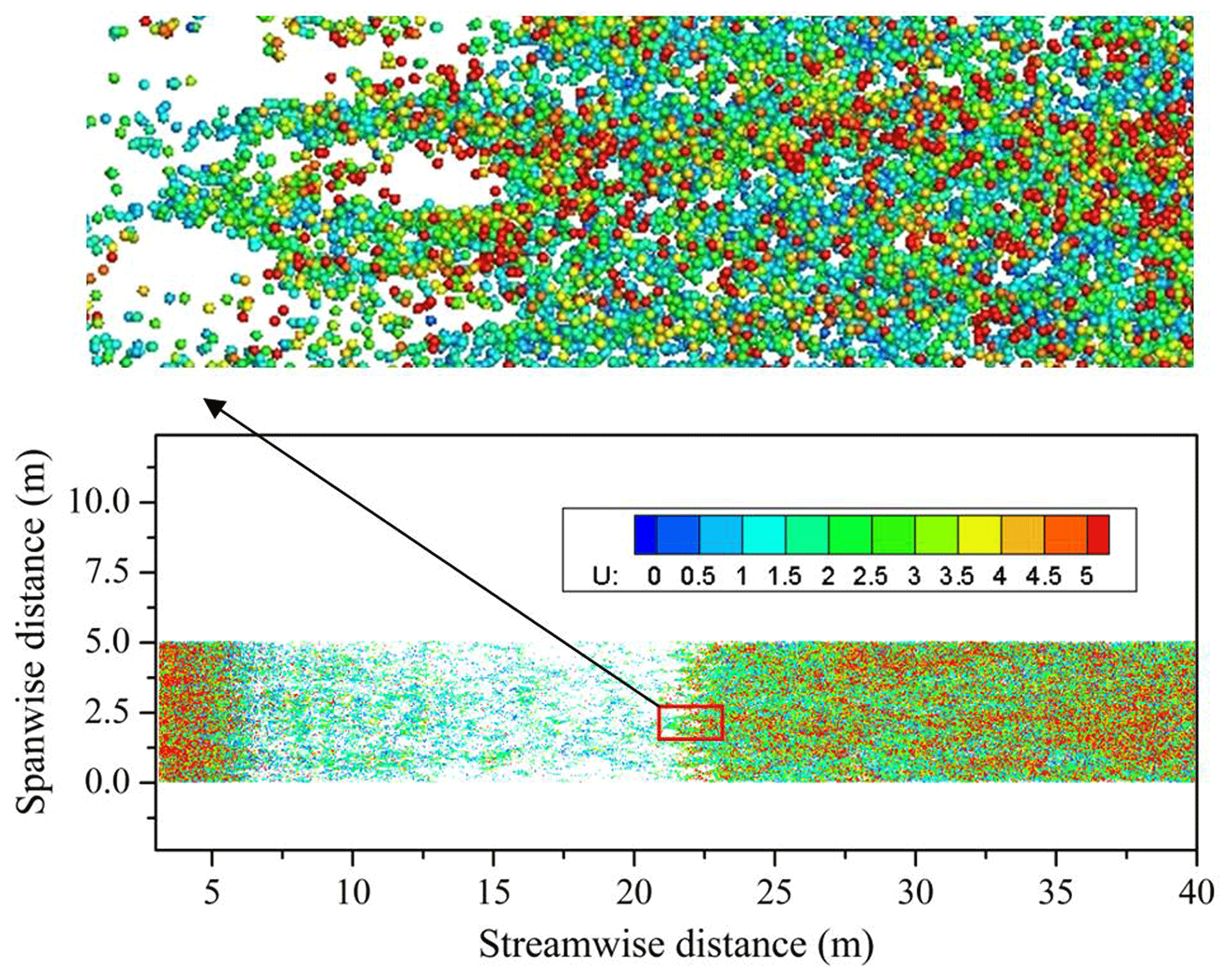
Figure 9The top view of the particle positions of the wind-blown sand in the presence of SCBs, where U represents the speed of the particles (uτ=0.6 m s−1; N=5–20 m).
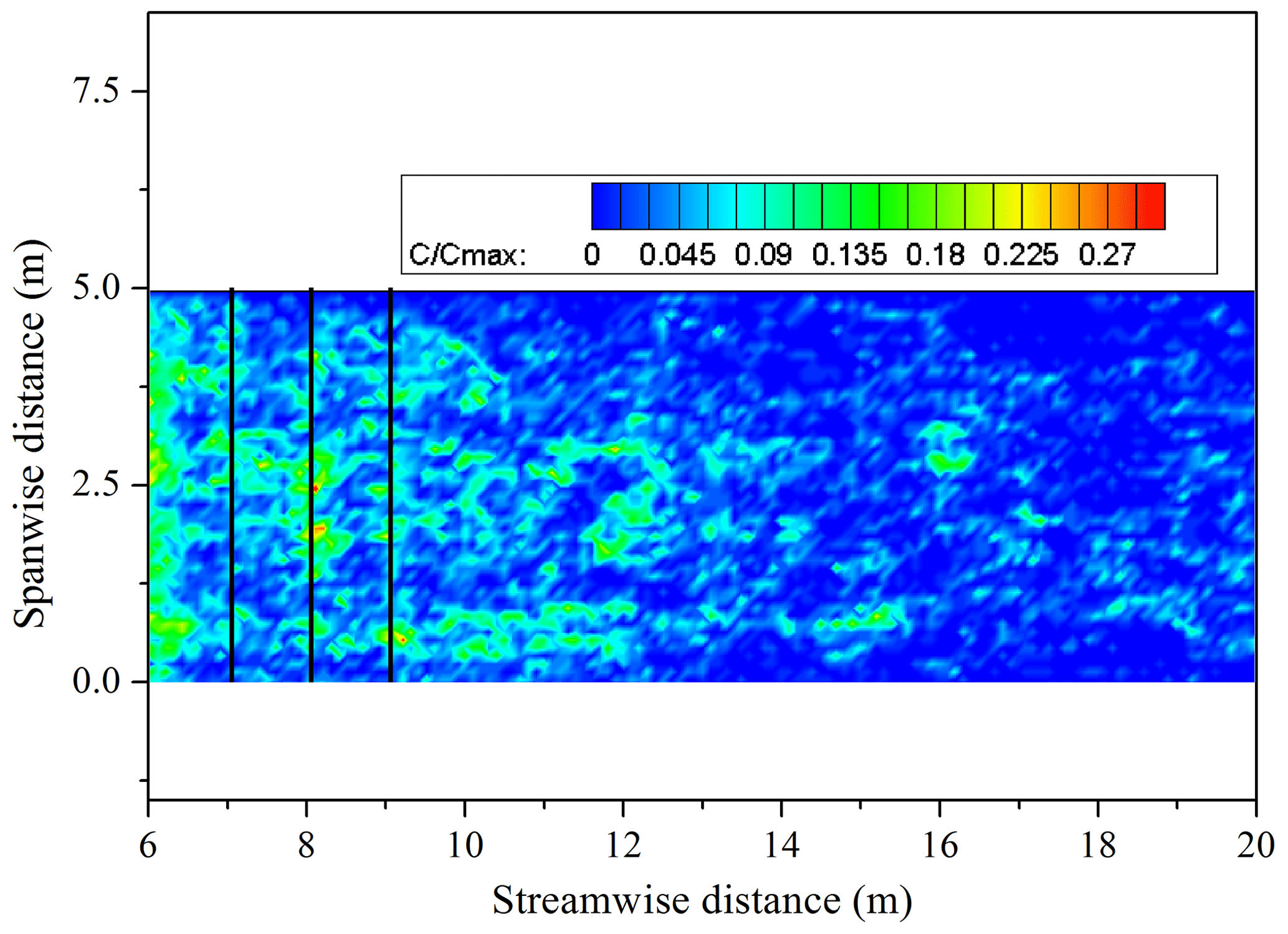
Figure 10The top view of the sand concentrations in the regions of the SCBs, where C represents the particle concentrations and Cmax represents the maximum particle concentrations (uτ=0.6 m s−1; N=5–20 m). The black lines represent the schematic diagram of the side of SCBs.
Furthermore, we analyze the effect of sand particles on the wind speed in the sand-laden flow. The streamwise wind speed of the sand-laden flow at the different laying length cases (N=5–10, 5–20, 5–30 m) under the same friction wind speed is plotted in Fig. 11a and b. Meanwhile, for the convenience of comparison, the streamwise wind speed under the same laying length (N=5–20 m) in the sand-laden flow and the clean airflow are plotted in Fig. 11c and d. Figure 11a and c correspond to the wind speed at a height of 0.1 m, while Fig. 11b and d correspond to the wind speed at a height of 0.2 m. From Fig. 11a–d, we can still see an oscillating decrease in the wind speed in the SCBs of the sand-laden flow. The streamwise wind speed behind the SCBs in the sand-laden flow is significantly lower than that in the clean airflow. Obviously, the presence of sand particles does reduce the wind speed. However, the change in wind speed in the SCBs between the sand-laden flow and the clean airflow is not obvious because there are fewer sand particles in the SCBs than behind the SCBs, which has less effect on the overall wind speed.
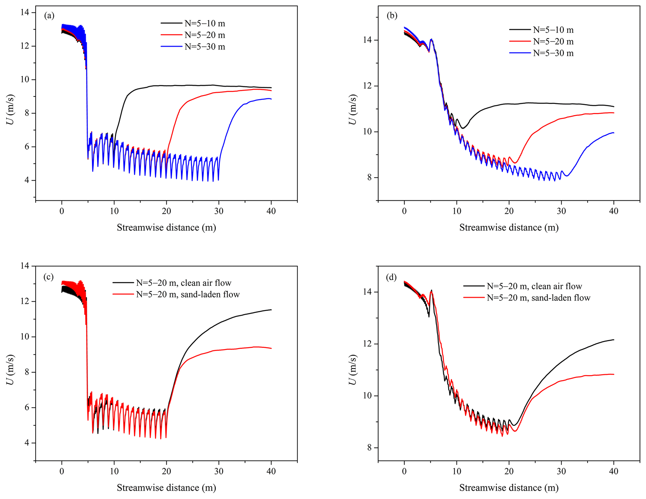
Figure 11The streamwise wind speed in the sand-laden flow containing the SCBs at the height of 0.1 m (a) and the height of 0.2 m (b) (uτ=0.6 m s−1; N=5–10, 5–20, 5–30 m). A comparison of the streamwise wind speed between the clean airflow and the sand-laden flow at a height of 0.1 m (c) and a height of 0.2 m (d) (uτ=0.6 m s−1; N=5–20 m) is also shown.
4.3 Effect of the laying length on the sand transport rate
The effect of the different laying length cases (N=5–10, 5–20, 5–30 m) on the sand transport rate under the same friction wind speed is plotted in Fig. 12. It can be seen from Fig. 12 that the sand transport rate in the SCBs is very low, and as the laying length increases, the sand transport rate in the SCBs decreases. In the case of N=5–30 m, the sand transport rate in some regions has been reduced to zero. Therefore, this result once again shows that the laying length of the SCBs can be optimized, and we can reduce the laying cost while maintaining the effect of the SCBs. Our model can give the minimum laying length according to the actual parameters, especially on both sides of the desert highway. At the same time, we notice that the sand transport rate will increase rapidly and then reach a stable state behind the SCBs. It is obvious that when N=5–30 m, the value of the sand transport rate at the stable stage behind the SCBs is significantly lower than the other results of N=5–10 m and N=5–20 m. We also notice that the longer the laying lengths are, the lower the sand transport rate in the stable stage behind the SCBs will be. This result corresponds to the result shown in Fig. 8. Our results indicate that when sandy land is wide, the discontinuous laying method can be considered. That means that the minimum laying length must be determined first, and then the distance between each minimum laying length can be set as needed. In this way, the sand transport rate can be reduced in sections. This is another potential application of our model.
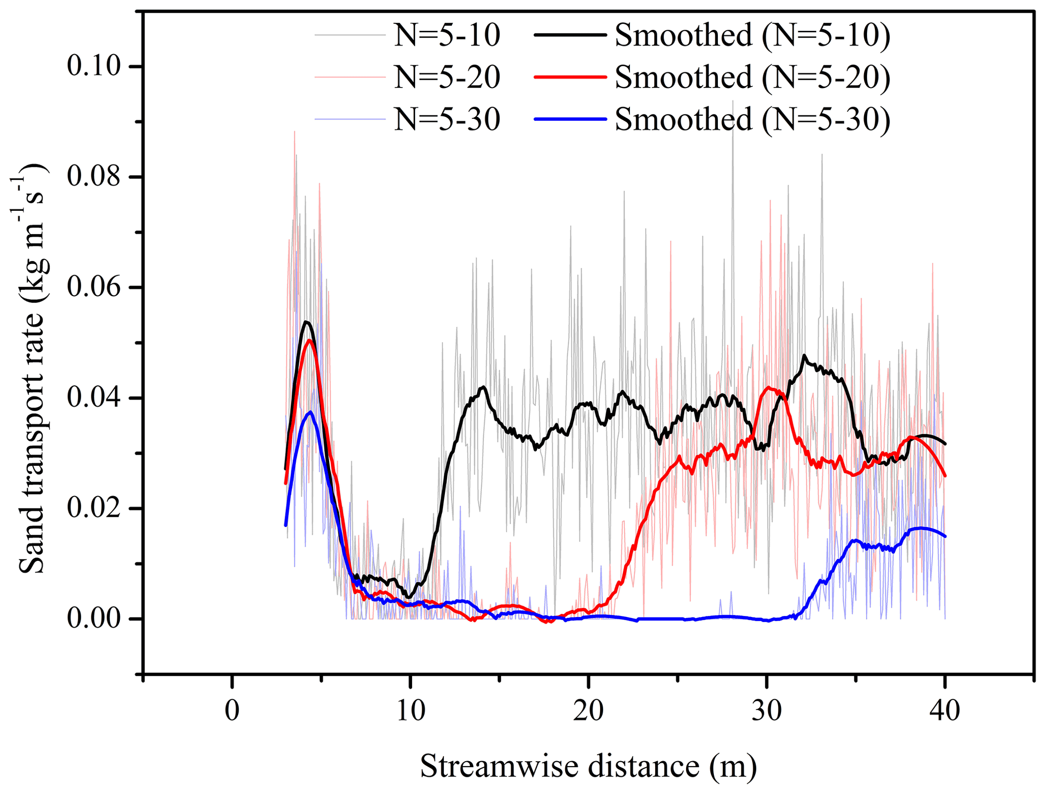
Figure 12The streamwise sand transport rate in the different laying length cases (uτ=0.6 m s−1; N=5–10, 5–20, 5–30 m). Dark lines are the result of smoothing.
4.4 Particle positions under different friction wind speeds
The above analysis is based on the calculation case when the friction wind speed is 0.6 m s−1, and the sand particles can easily penetrate the SCBs when the wind speed is large. When the friction wind speed is small, the inhibition effect of the SCBs on wind-blown sand will become more obvious, and the movement behavior of sand particles will change. We focused on the effect of SCBs on the wind-blown sand within 2 to 5 s after the sand-laden flow is saturated. We plot the top view of the particle positions at different moments (t=2, 5 s) when the friction wind speed is 0.3 and 0.6 m s−1 in Figs. 13 and 14, respectively. The initial value of time t in Figs. 13 and 14 is when sand particles are added. The results show that when the wind speed is small, the sand particles cannot penetrate the SCBs. There is no obvious sand movement in the SCBs, and stable wind-blown sand cannot be formed behind the SCBs. With the passage of time, the wind-blown sand behind the SCBs gradually disappears. It is worth noting that aerodynamic entrainment is not considered in our model. This is a considerable limitation of our model in the simulation of wind erosion in the presence of SCBs. Therefore, a more reasonable situation is that when the wind speed behind the SCBs returns to the fluid threshold, this part of the wind-blown sand should still develop. On the one hand, when the wind speed is relatively small, the sand particles cannot completely penetrate the regions of the SCBs and cannot continuously provide the impact particles to form the wind-blown sand behind the SCBs. On the other hand, the SCBs affect the surface wind speed behind it, thus also affecting the continuous formation of wind-blown sand. When the wind speed is relatively high, the sand particles can penetrate the SCBs. With increasing laying length, although the inhibition effect on wind-blown sand is more obvious, stable wind-blown sand will still be formed behind the SCBs. We think that when the laying length of the SCBs is fixed, whether the wind speed will decrease below the impact threshold or the fluid threshold is the key to determining whether the sand particles can penetrate the SCBs and form stable wind-blown sand behind the SCBs. To present this phenomenon more clearly, we have animated this process, as shown in the Supplement (Video 1 and Video 2). In actual anti-desertification projects, the minimum laying length of the SCBs can be determined by our model according to the local maximum friction wind speed.
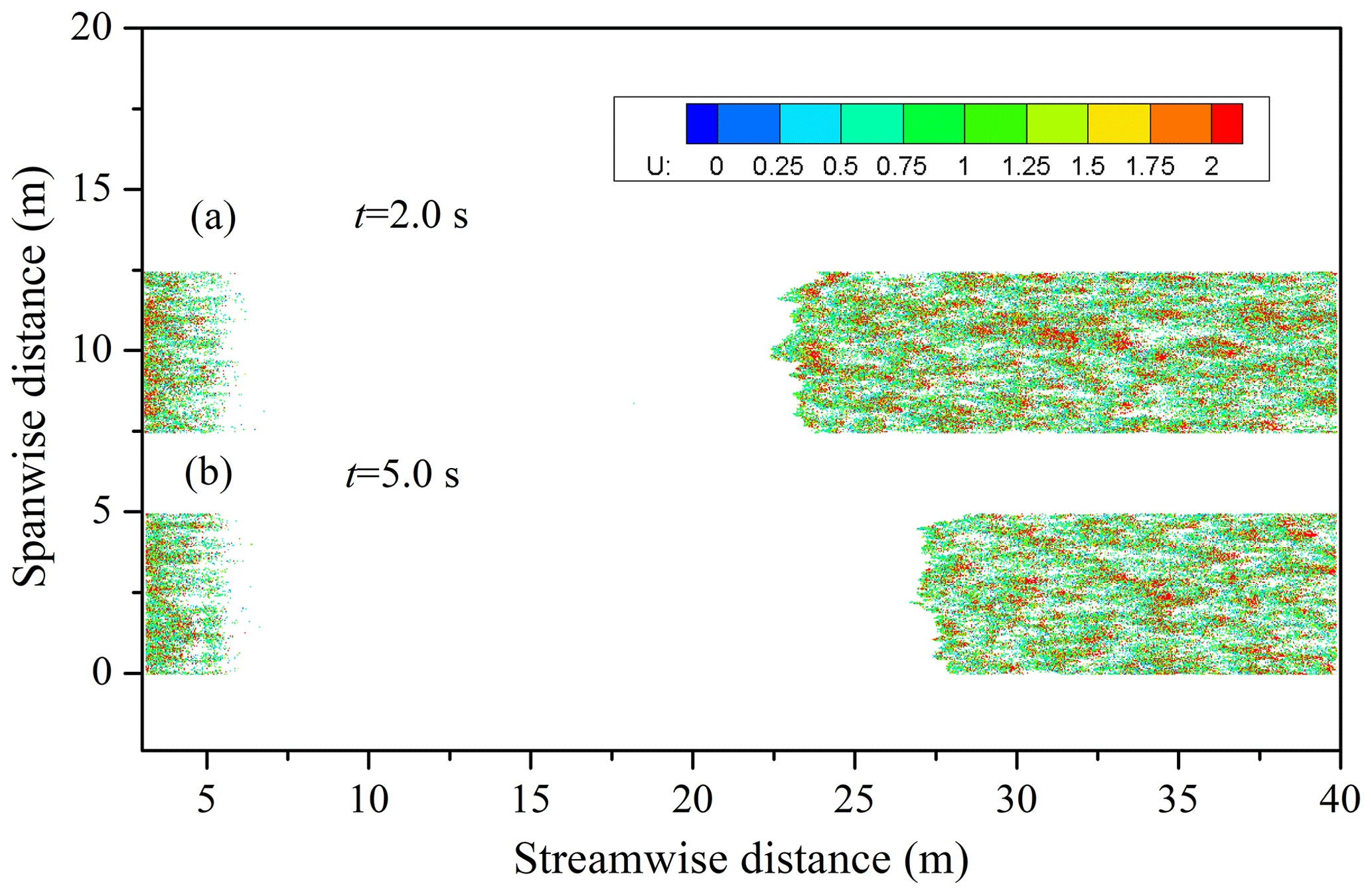
Figure 13The top view of the particle positions of the wind-blown sand in the presence of SCBs at t=2.0 s (a) and t=5.0 s (b), where U represents the speed of the particles (uτ=0.3 m s−1; N=5–20 m). The y coordinates are correspondingly shifted up by 7.5 m in (a).
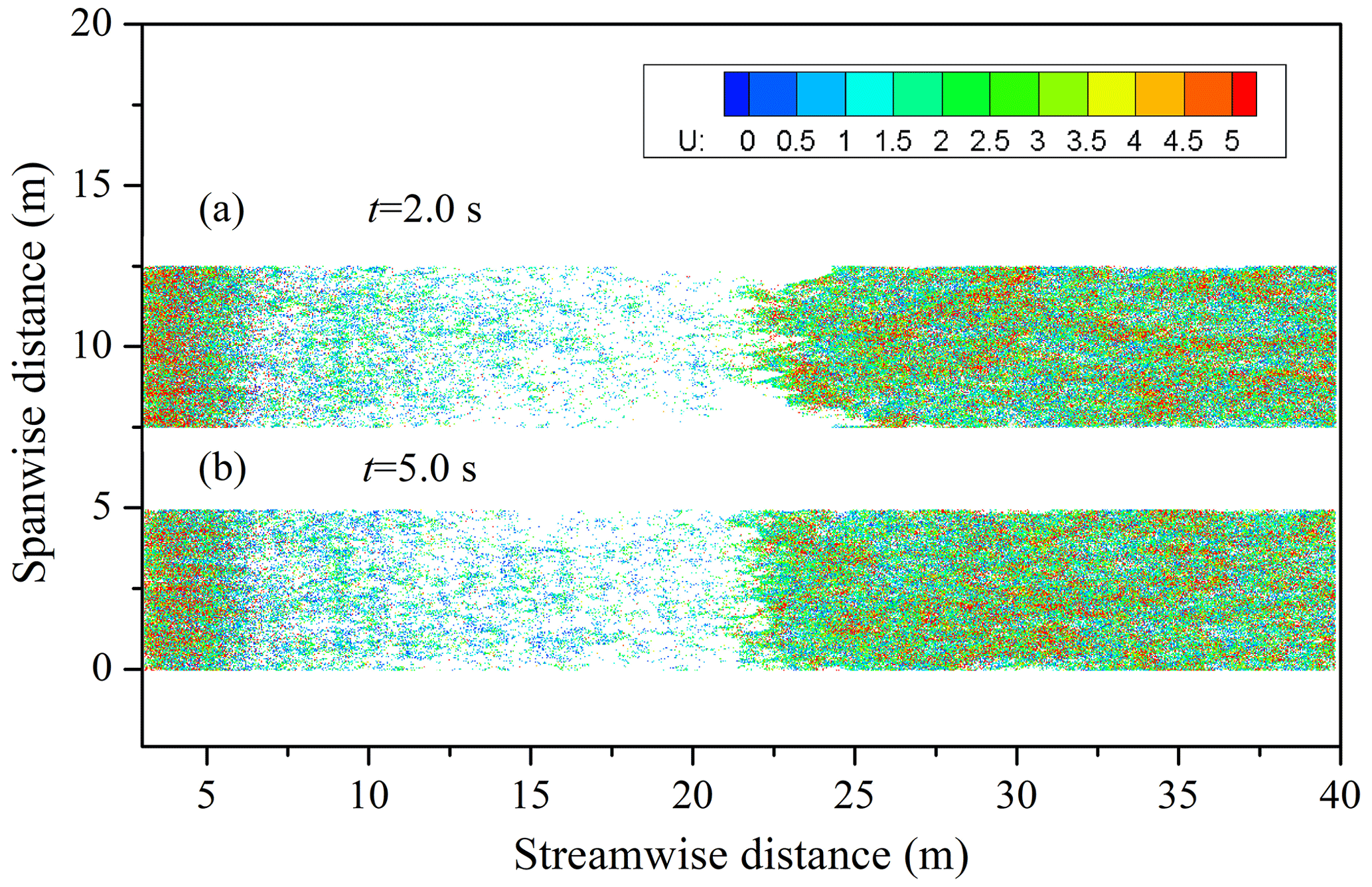
Figure 14The top view of the particle positions of the wind-blown sand in the presence of SCBs at t=2.0 s (a) and t=5.0 s (b), where U represents the speed of the particles (uτ=0.6 m s−1; N=5–20 m). The y coordinates are correspondingly shifted up by 7.5 m in (a).
In this paper, a three-dimensional wind-blown-sand coupling model in the presence of SCBs was established. The model was verified from the following aspects: (1) spatial distribution of the sand transport rate; (2) morphological characteristics of the sand streamer resulting from the instantaneous fields; and (3) changes in the thickness of the boundary layer before and after the SCBs. From this model, the inhibition effect of SCBs on wind-blown sand was studied qualitatively, and the sensitivity of eolian sand erosion to the laying length was investigated. The results showed that the wind speed in the SCBs of the clean airflow or the sand-laden flow decreases in an oscillating manner, which has not been revealed by previous studies. Moreover, the longer the laying lengths of the SCBs are, the lower the wind speed and the sand transport rate in the stable stage behind the SCBs will be, which may provide theoretical support for the minimum laying length of SCBs in anti-desertification projects. More importantly, we found that the concentration of sand particles near the side of SCBs is higher than that in its central region, which is consistent with previous research. This explains why the boundary of the SCBs tends to be buried in sandy land and loses its effect after long working hours. Our results also indicated that whether the wind speed will decrease below the impact threshold or the fluid threshold is the key factor affecting whether sand particles can penetrate the SCBs and form stable wind-blown sand behind the SCBs under the same conditions. Although our model has been able to reveal the inhibition effect of the SCBs on wind-blown sand, there are still some aspects that need improvement, such as aerodynamic entrainment, particle deposition on the SCB, and collision between the sand particles and the SCBs. The resolution of these issues is expected to reveal more details of particle deposition around the SCBs, which needs in-depth study. The size of the SCB used in our model is fixed. In future work, we plan to analyze the effect of different heights and widths of the SCB on eolian sand erosion and discuss the reasons for the difference in heights between the SCB and other obstacles, such as sand fences. Another aspect worth noting is that some additional factors, such as terrain and surface roughness, will affect SCB performance in anti-desertification projects, so the influence of these factors should be considered in the future. Using the proposed model, our work significantly analyzed some results that are seemingly simple but lack a theoretical basis from the perspective of turbulence.
All relevant code and data used to generate the figures in this paper can be made available upon reasonable request to the author by sending an email to the following address: hjhuang@usst.edu.cn.
Video 1 and Video 2 can be downloaded at the following link: https://doi.org/10.5281/zenodo.6937805 (Huang, 2022).
The supplement related to this article is available online at: https://doi.org/10.5194/esurf-11-167-2023-supplement.
The author has declared that there are no competing interests.
Publisher's note: Copernicus Publications remains neutral with regard to jurisdictional claims in published maps and institutional affiliations.
The author would like to thank the Center for Analysis and Prediction of Storms (CAPS) at the University of Oklahoma for providing the original ARPS code. The author also thankful to Andreas Baas for his careful help with the manuscript and to Catherine Le Ribault and the anonymous reviewer for their helpful comments.
This research was supported by grants from the National Natural Science Foundation of China (grant no. 12002119) and the Opening Foundation of MOE Engineering Research Center of Desertification and Blown-sand Control, Beijing Normal University (2021-B-4).
This paper was edited by Andreas Baas and reviewed by Catherine Le Ribault and one anonymous referee.
Anderson, R. S. and Haff, P.: Wind modification and bed response during saltation of sand in air, Acta Mech. Supp. 1, 21–51, https://doi.org/10.1007/978-3-7091-6706-9_2, 1991.
Anderson, R. S., Sørensen, M., and Willetts, B. B.: A review of recent progress in our understanding of aeolian sediment transport, Acta Mech. Supp., 1, 1–19, https://doi.org/10.1007/978-3-7091-6706-9_1, 1991.
Baas, A. C. W. and Sherman, D.: Formation and behavior of aeolian streamers, J. Geophys. Res.-Earth, 110, F03011, https://doi.org/10.1029/2004JF000270, 2005.
Bitog, J., Lee, I. B., Shin, M. H., Hong, S. W., Hwang, H. S., Seo, I. H., Yoo, J. I., Kwon, K. S., Kim, Y. H., and Han, J. W.: Numerical simulation of an array of fences in Saemangeum reclaimed land, Atmos. Environ. 43, 4612–4621, https://doi.org/10.1016/j.atmosenv.2009.05.050, 2009.
Bo, T. L., Ma, P., and Zheng, X. J.: Numerical study on the effect of semi-buried straw checkerboard sand barriers belt on the wind speed, Aeolian Res. 16, 101–107, https://doi.org/10.1016/j.aeolia.2014.10.002, 2015.
Bouvet, T., Wilson, J., and Tuzet, A.: Observations and modeling of heavy particle deposition in a windbreak flow, J. Appl. Meteorol. Clim., 45, 1332–1349, https://doi.org/10.1175/JAM2382.1, 2006.
Carneiro, M. V., Araújo, N. A., Pähtz, T., and Herrmann, H. J.: Midair collisions enhance saltation, Phys. Rev. Lett. 111, 058001, https://doi.org/10.1103/PhysRevLett.111.058001, 2013.
Chang, Z., Zhong, S., Han, F., and Liu, H.: Research of the suitable row spacing on clay barriers and straw barriers, J. Desert Res., 20, 455–457, 2000.
Chen, B., Cheng, J., Xin, L., and Wang, R.: Effectiveness of hole plate-type sand barriers in reducing aeolian sediment flux: Evaluation of effect of hole size, Aeolian Res., 38, 1–12, https://doi.org/10.1016/j.aeolia.2019.03.001, 2019.
Cheng, J. J. and Xue, C. X.: The sand-damage-prevention engineering system for the railway in the desert region of the Qinghai-Tibet plateau, J. Wind Eng. Ind. Aerod., 125, 30–37, https://doi.org/10.1016/j.jweia.2013.11.016, 2014.
Cheng, J. J., Lei, J. Q., Li, S. Y., and Wang, H. F.: Disturbance of the inclined inserting-type sand fence to wind-sand flow fields and its sand control characteristics, Aeolian Res., 21, 139–150, https://doi.org/10.1016/j.aeolia.2016.04.008, 2016.
Cheng, N. S.: Simplified settling velocity formula for sediment particle, J. Hydraul. Eng. 123, 149–152, https://doi.org/10.1061/(ASCE)0733-9429(1997)123:2(149), 1997.
Dai, Y., Dong, Z., Li, H., He, Y., Li, J., and Guo, J.: Effects of checkerboard barriers on the distribution of aeolian sandy soil particles and soil organic carbon, Geomorphology, 338, 79–87, https://doi.org/10.1016/j.geomorph.2019.04.016, 2019.
Dong, Z., Fryrear, D., and Gao, S.: Modeling the roughness effect of blown-sand-controlling standing vegetation in wind tunnel, J. Desert Res., 20, 260–263, 2000.
Dupont, S., Bergametti, G., Marticorena, B., and Simoëns, S.: Modeling saltation intermittency, J. Geophys. Res.-Atmos., 118, 7109–7128, https://doi.org/10.1002/jgrd.50528, 2013.
Dupont, S., Bergametti, G., and Simoëns, S.: Modeling aeolian erosion in presence of vegetation, J. Geophys. Res.-Earth, 119, 168–187, https://doi.org/10.1002/2013JF002875, 2014.
Germano, M., Piomelli, U., Moin, P., and Cabot, W. H.: A dynamic subgrid-scale eddy viscosity model, Phys. Fluids A, 3, 1760–1765, https://doi.org/10.1063/1.857955, 1991.
Hatanaka, K. and Hotta, S.: Finite element analysis of air flow around permeable sand fences, Int. J. Numer. Meth. Fluids, 24, 1291–1306, https://doi.org/10.1002/(SICI)1097-0363(199706)24:12<1291::AID-FLD560>3.0.CO;2-N, 1997.
Huang, H.: Videos in egusphere-2022-714, Zenodo [video], https://doi.org/10.5281/zenodo.6937805, 2022.
Huang, H. J.: Modeling the effect of saltation on surface layer turbulence, Earth Surf. Proc. Land., 45, 3943–3954, https://doi.org/10.1002/esp.5013, 2020.
Huang, H. J., Bo, T. L., and Zheng, X. J.: Numerical modeling of wind-blown sand on Mars, Eur. Phys. J. E, 37, 80, https://doi.org/10.1140/epje/i2014-14080-7, 2014.
Huang, H. J., Bo, T. L., and Zhang, R.: Exploration of splash function and lateral velocity based on three-dimensional mixed-size grain/bed collision, Granul. Matter, 19, 73, https://doi.org/10.1007/s10035-017-0759-9, 2017.
Huang, N. and Wang, Z. S.: The formation of snow streamers in the turbulent atmosphere boundary layer, Aeolian Res., 23, 1–10, https://doi.org/10.1016/j.aeolia.2016.09.002, 2016.
Huang, N., Zhang, Y., and D'Adamo, R.: A model of the trajectories and midair collision probabilities of sand particles in a steady state saltation cloud, J. Geophys. Res.-Atmos., 112, D08206, https://doi.org/10.1029/2006JD007480, 2007.
Huang, N., Xia, X., and Tong, D.: Numerical simulation of wind sand movement in straw checkerboard barriers, Eur. Phys. J. E, 36, 99, https://doi.org/10.1140/epje/i2013-13099-6, 2013.
Inoue, M. and Pullin, D.: Large-eddy simulation of the zero-pressure-gradient turbulent boundary layer up to Reθ=O (1012), J. Fluid Mech., 686, 507–533, https://doi.org/10.1017/jfm.2011.342, 2011.
Kok, J. F. and Renno, N. O.: A comprehensive numerical model of steady state saltation (COMSALT), J. Geophys. Res.-Atmos., 114, D17204, https://doi.org/10.1029/2009JD011702, 2009.
Kok, J. F., Parteli, E. J., Michaels, T. I., and Karam, D. B.: The physics of wind-blown sand and dust, Rep. Prog. Phys., 75, 106901, https://doi.org/10.1088/0034-4885/75/10/106901, 2012.
Lee, J. and Lee, C.: Modification of particle-laden near-wall turbulence: effect of Stokes number, Phys. Fluids, 27, 023303, https://doi.org/10.1063/1.4908277, 2015.
Li, B. and Sherman, D. J.: Aerodynamics and morphodynamics of sand fences: A review, Aeolian Res., 17, 33–48, https://doi.org/10.1016/j.aeolia.2014.11.005, 2015.
Li, B. W., Zhou, X. J., Huang, P. Z., Xu, X. W., Wang, Z. J., and Zhang, C. M.: Wind-Sand Damage and Its Control at Shaquanzi Section of Lan-xin Railway, Arid Zone Res., 15, 47–52, 1998.
Li, G., Wang, Z., and Huang, N.: A Snow Distribution Model Based on Snowfall and Snow Drifting Simulations in Mountain Area, J. Geophys. Res.-Atmos., 123, 7193–7203, https://doi.org/10.1029/2018JD028434, 2018.
Li, X., Xiao, H., He, M., and Zhang, J.: Sand barriers of straw checkerboards for habitat restoration in extremely arid desert regions, Ecol. Eng., 28, 149–157, https://doi.org/10.1016/j.ecoleng.2006.05.020, 2006.
Lima, I. A., Araújo, A. D., Parteli, E. J., Andrade, J. S., and Herrmann, H. J.: Optimal array of sand fences, Sci. Rep., 7, 45148, https://doi.org/10.1038/srep45148, 2017.
Lima, I. A., Parteli, E. J., Shao, Y. P., Andrade, J. S., Herrmann, H. J., and Araújo, A. D.: CFD simulation of the wind field over a terrain with sand fences: Critical spacing for the wind shear velocity, Aeolian Res., 43, 100574, https://doi.org/10.1016/j.aeolia.2020.100574, 2020.
Lund, T. S., Wu, X. H., and Squires, K. D.: Generation of turbulent inflow data for spatially-developing boundary layer simulations, J. Comput. Phys., 140, 233–258, https://doi.org/10.1006/jcph.1998.5882, 1998.
Ma, G. S. and Zheng, X. J.: The fluctuation property of blown sand particles and the wind-sand flow evolution studied by numerical method, Eur. Phys. J. E, 34, 54, https://doi.org/10.1140/epje/i2011-11054-3, 2011.
McEwan, I. and Willetts, B.: Numerical model of the saltation cloud, Acta Mech. Supp., 1, 53–66, https://doi.org/10.1007/978-3-7091-6706-9_3, 1991.
Murphy, P. J. and Hooshiari, H.: Saltation in water dynamics, J. Hydrol. Div., 108, 1251–1267, https://doi.org/10.1061/JYCEAJ.0005931, 1982.
Nepf, H. M.: Flow and transport in regions with aquatic vegetation, Annu. Rev. Fluid Mech., 44, 123–142, https://doi.org/10.1146/annurev-fluid-120710-101048, 2012.
Qiu, G. Y., Lee, I. B., Shimizu, H., Gao, Y., and Ding, G.: Principles of sand dune fixation with straw checkerboard technology and its effects on the environment, J. Arid. Environ., 56, 449–464, https://doi.org/10.1016/S0140-1963(03)00066-1, 2004.
Qu, J., Zu, R., Zhang, K., and Fang, H.: Field observations on the protective effect of semi-buried checkerboard sand barriers, Geomorphology, 88, 193–200, https://doi.org/10.1016/j.geomorph.2006.11.006, 2007.
Rice, M. A., Willetts, B. B., and McEwan, I.: An experimental study of multiple grain-size ejecta produced by collisions of saltating grains with a flat bed, Sedimentology, 42, 695–706, https://doi.org/10.1111/j.1365-3091.1995.tb00401.x, 1995.
Richter, D. H.: Turbulence modification by inertial particles and its influence on the spectral energy budget in planar Couette flow, Phys. Fluids, 27, 063304, https://doi.org/10.1063/1.4923043, 2015.
Santiago, J., Martin, F., Cuerva, A., Bezdenejnykh, N., and Sanz-Andres, A.: Experimental and numerical study of wind flow behind windbreaks, Atmos. Environ., 41, 6406–6420, https://doi.org/10.1016/j.atmosenv.2007.01.014, 2007.
Shao, Y. P. and Raupach, M.: The overshoot and equilibration of saltation, J. Geophys. Res.-Atmos., 97, 20559–20564, https://doi.org/10.1029/92JD02011, 1992.
Smagorinsky, J.: General circulation experiments with the primitive equations: I. The basic experiment, Mon. Weather Rev., 91, 99–164, https://doi.org/10.1175/1520-0493(1963)091<0099:GCEWTP>2.3.CO;2, 1963.
Vinkovic, I., Aguirre, C., Ayrault, M., and Simoëns, S.: Large-eddy simulation of the dispersion of solid particles in a turbulent boundary layer, Bound.-Lay. Meteorol., 121, 283–311, https://doi.org/10.1007/s10546-006-9072-6, 2006.
Wang, T., Qu, J. J., and Niu, Q. H.: Comparative study of the shelter efficacy of straw checkerboard barriers and rocky checkerboard barriers in a wind tunnel, Aeolian Res., 43, 100575, https://doi.org/10.1016/j.aeolia.2020.100575, 2020.
Wang, X.: Discussion of sand hazard control along the Wu-Ji railway line, J. Desert Res., 16, 204–206, 1996.
Wang, X., Chen, G., Han, Z., and Dong, Z.: The benefit of the prevention system along the desert highway in Tarim Basin, J. Desert Res., 19, 120–127, 1999.
Wang, X., Zhang, C., Hasi, E., and Dong, Z.: Has the Three Norths Forest Shelterbelt Program solved the desertification and dust storm problems in arid and semiarid China?, J. Arid. Environ., 74, 13–22, https://doi.org/10.1016/j.jaridenv.2009.08.001, 2010.
Wang, Z. T. and Zheng, X. J.: A Simple Model for Calculating Measurements of Straw Checkerboard Barriers, J. Desert Res., 22, 229–232, 2002.
Werner, B.: A steady-state model of wind-blown sand transport, J. Geol., 98, 1–17, https://doi.org/10.1086/629371, 1990.
Wilson, J. D.: Oblique, stratified winds about a shelter fence. Part II: Comparison of measurements with numerical models, J. Appl. Meteorol., 43, 1392–1409, https://doi.org/10.1175/JAM2147.1, 2004.
Xu, B., Zhang, J., Huang, N., Gong, K., and Liu, Y.: Characteristics of turbulent aeolian sand movement over straw checkerboard barriers and formation mechanisms of their internal erosion form, J. Geophys. Res.-Atmos., 123, 6907–6919, https://doi.org/10.1029/2017JD027786, 2018.
Xu, J. L., Pei, Z. Q., and Wang, R. H.: Exploration of the width of the semi-buried straw checkerboard sand barriers belt, J. Desert Res., 2, 16–23, 1982.
Xu, X., Hu, Y., and Pan, B.: Analysis of the protective effect of various measures of combating drifting sand on the Tarim Desert Highway, Arid Zone Res., 15, 21–26, 1998.
Xue, M., Droegemeier, K., Wong, V., Shapiro, A., and Brewster, K.: Advanced Regional Prediction System (ARPS) version 4.0 user's guide, Center for Analysis and Prediction of Storms, University of Oklahoma, 119–120, https://arps.caps.ou.edu (last access: 11 March 2023), 1995.
Xue, M., Droegemeier, K. K., and Wong, V.: The Advanced Regional Prediction System (ARPS) – A multi-scale nonhydrostatic atmospheric simulation and prediction model. Part I: Model dynamics and verification, Meteorol. Atmos. Phys., 75, 161–193, https://doi.org/10.1007/s007030070003, 2000.
Xue, M., Droegemeier, K. K., Wong, V., Shapiro, A., Brewster, K., Carr, F., Weber, D., Liu, Y., and Wang, D.: The Advanced Regional Prediction System (ARPS) – A multi-scale nonhydrostatic atmospheric simulation and prediction tool. Part II: Model physics and applications, Meteorol. Atmos. Phys., 76, 143–165, https://doi.org/10.1007/s007030170027, 2001.
Yang, A.: Closing sandy land to establish vegetation along a desert railway line, J. Desert Res., 15, 308–311, 1995.
Zhang, C., Li, Q., Zhou, N., Zhang, J., Kang, L., Shen, Y., and Jia, W.: Field observations of wind profiles and sand fluxes above the windward slope of a sand dune before and after the establishment of semi-buried straw checkerboard barriers, Aeolian Res., 20, 59–70, https://doi.org/10.1016/j.aeolia.2015.11.003, 2016.
Zhang, K. C., Qu, J. J., Liao, K. T., Niu, Q. H., and Han, Q. J.: Damage by wind-blown sand and its control along Qinghai-Tibet Railway in China, Aeolian Res., 1, 143–146, https://doi.org/10.1016/j.aeolia.2009.10.001, 2010.
Zhang, S., Ding, G. D., Yu, M. H., Gao, G. L., Zhao, Y. Y., Wu, G. H., and Wang, L.: Effect of straw checkerboards on wind proofing, sand fixation, and ecological restoration in shifting Sandy Land, Int. J. Environ. Res., 15, 2184, https://doi.org/10.3390/ijerph15102184, 2018.
Zheng, X. J.: Mechanics of wind-blown sand movements, Springer Science & Business Media, https://doi.org/10.1007/978-3-540-88254-1, 2009.
Zhou, Y. H., Li, W. Q., and Zheng, X. J.: Particle dynamics method simulations of stochastic collisions of sandy grain bed with mixed size in aeolian sand saltation, J. Geophys. Res.-Atmos., 111, D15108, https://doi.org/10.1029/2005JD006604, 2006.
Zou, X. Y., Cheng, H., Zhang, C. L., and Zhao, Y. Z.: Effects of the Magnus and Saffman forces on the saltation trajectories of sand grain, Geomorphology, 90, 11–22, https://doi.org/10.1016/j.geomorph.2007.01.006, 2007.