the Creative Commons Attribution 4.0 License.
the Creative Commons Attribution 4.0 License.
 | 21 Jul 2023
Modeling the spatially distributed nature of subglacial sediment transport and erosion
Leif Anderson
Frédéric Herman
Glaciers expel sediment as they melt, in addition to ice and water. As a result, changing glacier dynamics and melt produce changes to glacier erosion and sediment discharge, which can impact the landscape surrounding retreating glaciers, as well as communities and ecosystems downstream. Currently, numerical models that transport subglacial sediment on sub-hourly to decadal scales are one-dimensional, usually along a glacier's flow line. Such models have proven useful in describing the formation of glacial landforms, the impact of sediment transport on glacier dynamics, and the interactions among climate, glacier dynamics, and erosion. However, these models omit the two-dimensional spatial distribution of sediment and its impact on sediment connectivity – the movement of sediment between its detachment in source areas and its deposition in sinks. Here, we present a numerical model that fulfills a need for predictive frameworks that describe subglacial sediment discharge in two spatial dimensions (x and y) over time. SUGSET_2D evolves a two-dimensional subglacial till layer in response to bedrock erosion and changing sediment transport conditions. Numerical experiments performed using an idealized alpine glacier illustrate the heterogeneity in sediment transport and bedrock erosion below the glacier. An increase in sediment discharge follows increased glacier melt, as has been documented in field observations and other numerical experiments. We also apply the model to a real alpine glacier, Griesgletscher in the Swiss Alps, where we compare outputs with annual measurements of sediment discharge. SUGSET_2D accurately reproduces the general quantities of sediment discharge and the year-to-year sediment discharge pattern measured at the glacier terminus. The model's ability to match the measured data depends on the tunable sediment grain size parameter, which controls subglacial sediment transport capacity. Smaller grain sizes allow sediment transport to occur in regions of the bed with reduced water flow and channel size, effectively increasing sediment connectivity into the main channels. The model provides the essential components of modeling subglacial sediment discharge on seasonal to decadal timescales and reveals the importance of including spatial heterogeneities in water discharge and sediment transport in both the x and y dimensions in evaluating sediment discharge.
- Article
(5654 KB) - Full-text XML
- BibTeX
- EndNote


Increasing glacier ablation perturbs the processes through which glaciers erode bedrock and supply sediment downstream (e.g., Church and Ryder, 1972; Lane et al., 2017; Delaney and Adhikari, 2020). Changing sediment discharge from glaciers in alpine and polar landscapes impacts many social and Earth systems (Milner et al., 2017; Li et al., 2021). Thus, predictive models are needed to understand the response of these systems to glacier retreat. In alpine environments, increased sediment discharge leads to the more rapid filling of proglacial reservoirs (Thapa et al., 2005; Li et al., 2022) and abrasion of hydropower infrastructure (e.g., Felix et al., 2016). The flux of sediment from glaciers also dramatically alters alpine ecosystems (Milner et al., 2017) and occurs when high melt extends up-glacier, thus mobilizing sediment in new areas (Lane et al., 2017; Delaney and Adhikari, 2020; Li et al., 2021). In Arctic environments, increased sediment discharge can affect biogeochemical cycles given that sediments may carry phosphorus and iron (Bhatia et al., 2013; Hawkings et al., 2014). These elements are limiting nutrients in the oceanic ecosystem, so any change to sediment discharge from glaciers and ice sheets therefore alters Arctic ecosystems (Wadham et al., 2019).
Generally, two processes determine the sediment discharge below glaciers: one process adds sediment, and the other removes sediment from subglacial till layers (Fig. 1; Brinkerhoff et al., 2017; Delaney et al., 2019). Bedrock erosion adds material to the subglacial till layer. This is accomplished by quarrying, when pressure differentials on opposing sides of obstacles cause fractures to expand and rock to detach (Iverson, 1990, 2012; Alley et al., 1997; Hallet et al., 1996), and by abrasion, when debris embedded in the ice grinds bedrock as the glacier slides above (Hallet, 1979; Alley et al., 1997). Representation of these physical processes in models requires independent knowledge of a large number of parameters (see Ugelvig et al., 2018), so many researchers use empirical relationships that relate glacier sliding to glacier erosion (Humphrey and Raymond, 1994; Koppes et al., 2015; Herman et al., 2015; Cook et al., 2020). These relationships prove especially useful when applied over large temporal and spatial scales, for example, to explore the coupling of glacier erosion, climate, and tectonic uplift (e.g., Egholm et al., 2009; Prasicek et al., 2018; Herman et al., 2018; Prasicek et al., 2020; Seguinot and Delaney, 2021).
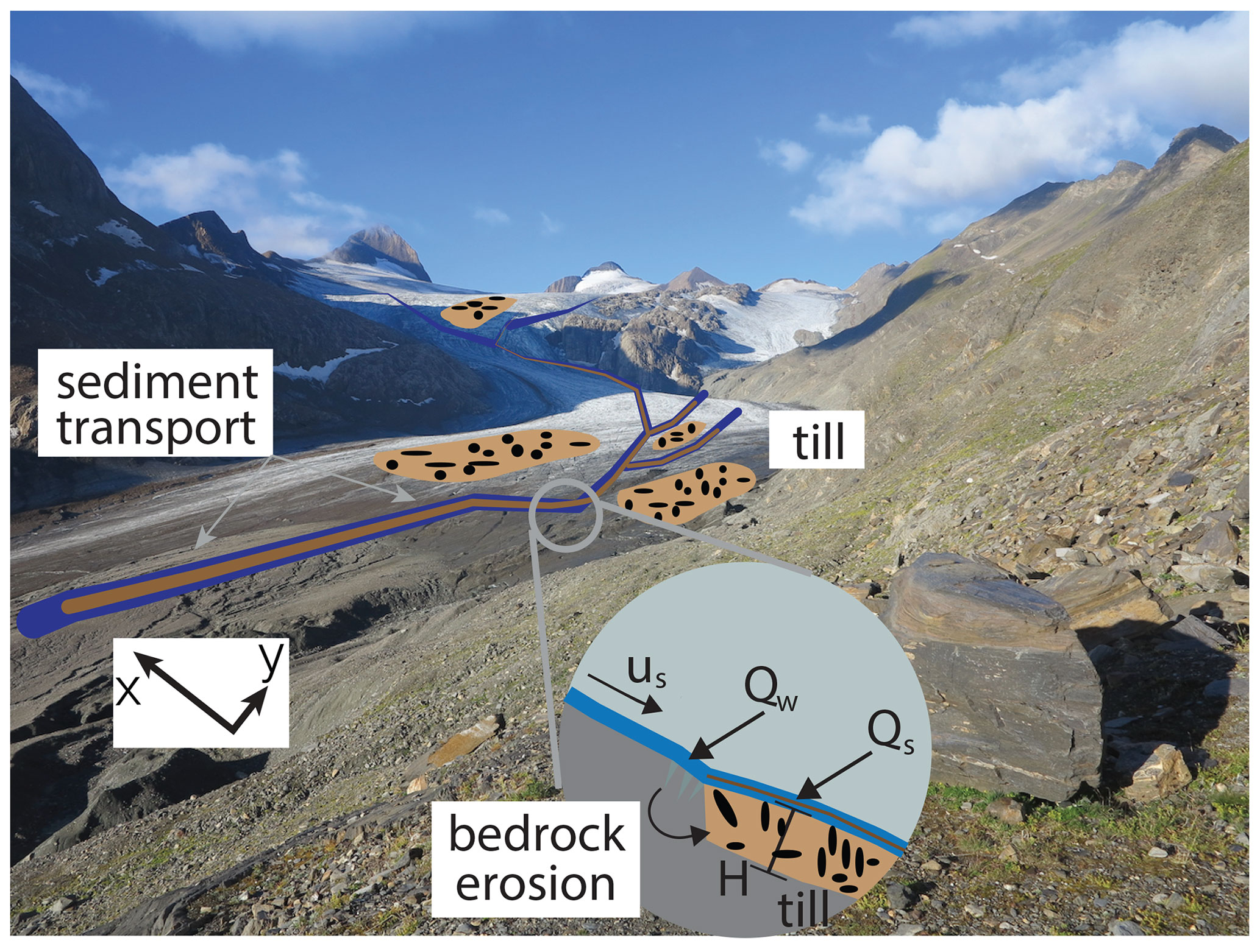
Figure 1Cartoon of erosional and sediment transport processes considered in the model overlaid on an image of Griesgletscher in 2016. Bedrock erosion scales with sliding speed (us) and adds material to the till layer with thickness (H), while water (Qw) transports sediment (Qs) fluvially if sediment persists in that location of the glacier bed and fluvial conditions are sufficient for transport. Photo credit: Ian Delaney.
Conversely, fluvial sediment transport mobilizes material from subglacial till layers (e.g., Walder and Fowler, 1994; Ng, 2000) or it may deposit the mobilized material in the till layers under certain hydraulic conditions (e.g., Beaud et al., 2018a; Hewitt and Creyts, 2019; Delaney and Anderson, 2022). As subglacial water velocity increases, the sediment of a given grain size is transported below the glacier, and this sediment may be deposited if the water velocity slows (e.g., Meyer-Peter and Müller, 1948; Paola and Voller, 2005). Sediment mobilization ceases when no sediment is present, and the system is supply-limited (e.g., Mao et al., 2014). Thus, fluvial sediment transport depends on both the subglacial hydraulic characteristics (e.g., Walder and Fowler, 1994) and the availability of sediment at the glacier bed (e.g., Willis et al., 1996; Swift et al., 2005).
Bedrock erosion and fluvial sediment transport vary depending on the characteristics of each glacier. Bedrock erosion processes tend to dominate sediment discharge below glaciers with minimal sediment storage, large concentrations of subglacial debris entrained at the glacier bed, and steep gradients (Hallet, 1979; Humphrey and Raymond, 1994; Herman et al., 2015, 2021; Ugelvig et al., 2018). Landscape evolution models that represent glacier landscapes illustrate the dominant role of erosional processes, as opposed to sediment transport processes, over geologic timescales (Harbor et al., 1988; Herman et al., 2011; Egholm et al., 2012). Over shorter timescales of months to decades, however, fluvial sediment transport often drives sediment discharge (e.g., Delaney et al., 2018b, 2019; Perolo et al., 2018).
The development of numerical models of subglacial sediment transport to date has mainly focused on processes acting in the down-glacier (e.g., x) dimension. To date, one-dimensional models have yielded insights into the creation of eskers (Beaud et al., 2018a; Hewitt and Creyts, 2019), the formation of subglacial canals through which water flows (Walder and Fowler, 1994; Ng, 2000; Kasmalkar et al., 2019), subglacial processes in overdeepenings (Creyts et al., 2013), and the behavior of tidewater glaciers (Brinkerhoff et al., 2017). Yet spatial heterogeneities in the distribution of sediment and sediment transport capacity (largely controlled by water velocity) commonly result in the water carrying less sediment than could be transported theoretically (e.g., Delaney et al., 2018b). As a result, reducing the modeled processes to one dimension omits key processes controlling sediment dynamics because subglacial water flows through spatially distributed networks of cavities and channels across the glacier bed (e.g., Werder et al., 2013). Therefore, describing subglacial sediment transport inherently lends itself to a discretization of bedrock erosion, sediment transport, water flow, and sediment availability in both the down-glacier and transverse dimensions (e.g., x and y).
Here, we present SUGSET_2D, a two-dimensional subglacial sediment transport model that includes sediment transport and bedrock erosion processes. We implement a routing scheme that transports sediment in x and y directions based on the local hydraulic potential gradient. Synthetic cases demonstrate the model's ability to reproduce known processes and yield insights into the spatially distributed processes responsible for subglacial sediment dynamics. We also apply the model to a real alpine glacier, Griesgletscher, in Switzerland, which has a record of subglacial sediment transport from the catchment from the period 2011 to 2016. The model was run with topography data and modeled hydrology from the glacier, and measured sediment discharge data were used to validate the model. Through these experiments, we identify key processes of sediment transport from subglacial environments.
The model presented here implements a hydraulic model and sediment routing scheme that translates many of the underpinnings of the one-dimensional subglacial sediment transport model presented in Delaney et al. (2019) to two dimensions. We describe hydraulic and sediment transport models, explain the implemented water and sediment routing scheme, and outline its numerical implementation in two dimensions.
2.1 Hydraulic model
SUGSET_2D requires a hydraulic model as a means to route sediment and water through the subglacial environment. The hydraulic model determines the sediment transport capacity of the subglacial water based upon the gradient of the hydraulic potential, channel size, and water flux (Table 1, Sect. 2.2; e.g., Walder and Fowler, 1994; Alley et al., 1997). The hydraulic model is based on the assumption that subglacial water flows along the hydraulic potential gradient, the weight of ice pressurizes water at the bed (Shreve, 1972), and the channel size varies over a substantially longer timescale compared to water discharge. This model includes characteristics of a Röthlisberger channel without explicitly describing properties such as creep closure and pressure melt of channel walls (Röthlisberger, 1972).
The gradient of the hydraulic potential of a subglacial channel Ψ (at a certain location and time) can be determined with a known hydraulic diameter Dh (a function of channel size and shape) and water discharge Qw. The gradient of the hydraulic potential can then be determined using the Darcy–Weisbach equation for fluid flow through a pipe:
where the density of water is ρw, the Darcy–Weisbach friction factor is fr, and the channel's cross-sectional geometry, which impacts water pressure, is accounted for by s (Hooke et al., 1990). We represent s as
where β is the central angle of the circular segment representing the channel edge. Smaller values of β result in broad channels and β=π results in a semicircular channel.
We assume that the hydraulic diameter Dh of the channel results from a characteristic water discharge , which is evaluated by the source percentile of water discharge over a certain time period sp and a response time of the channel size sa, that remains consistent throughout the model run (Table 1; Delaney et al., 2019).
We sum the prescribed melt rate up the glacier to define Qw, not considering englacial water storage. Percentile sp over a response time period prior to the time step sa is applied to Qw to evaluate a characteristic water discharge that represents the size of the conduit (hours to days; see Gimbert et al., 2016; de Fleurian et al., 2018; Delaney et al., 2019; Nanni et al., 2020). The timescales, sa, and characteristic water discharges (sp and ) responsible for changes in subglacial conduit size are poorly constrained, yet their impact can be intuited. For instance, short-lived increases in water discharge due to an hour of precipitation will not greatly impact the hydraulic diameter of the subglacial channel, whereas prolonged melt would increase the hydraulic diameter.
With data of representative water discharge below the glacier and the static hydraulic pressure gradient Ψ*, a representative hydraulic diameter Dh can be estimated. For a short period, such a Dh is assumed to be time-independent and is defined in Eq. (1):
where Ψ* is a representative gradient of the hydraulic potential at overburden pressure, evaluated using the Shreve potential gradient:
where zs and zb are surface and bed elevations, respectively, ρi is the density of ice, and g is the gravitational acceleration constant.
With knowledge of Dh, we insert the instantaneous value of Qw into Eq. (1) to evaluate the instantaneous gradient of the hydraulic potential Ψ. To prevent unreasonable water pressures when rapidly increases and Dh is small, the model limits the minimal hydraulic diameter to 0.3 m (Delaney et al., 2019).
2.2 Till layer model: bedrock erosion and sediment transport
SUGSET_2D simulates the evolution of a subglacial till layer, which we define as transportable sediment below the glacier produced through glacier erosion and fluvial sediment transport. Fluvial sediment transport, in supply- and transport-limited regimes, mobilizes and deposits sediment, removing or adding material from the till layer (Brinkerhoff et al., 2017; Delaney et al., 2019). Conversely, erosive processes such as abrasion and quarrying add material to the till layer. Note that we do not consider processes such as fluvial abrasion that appear to produce minimal sediment (Beaud et al., 2018b). To represent these processes, we implement the Exner equation (Fig. 2; Exner, 1920a, b; Paola and Voller, 2005), a mass conservation relationship, to solve for the till layer height given the erosive and fluvial conditions.
H is till thickness and t is time (Table 1). The first term on the right side of the equation represents fluvial sediment transport processes, where ∇⋅Qs represents sediment mobilization or deposition. The second term on the right side of the equation captures bedrock erosion processes, where is a bedrock erosion rate.
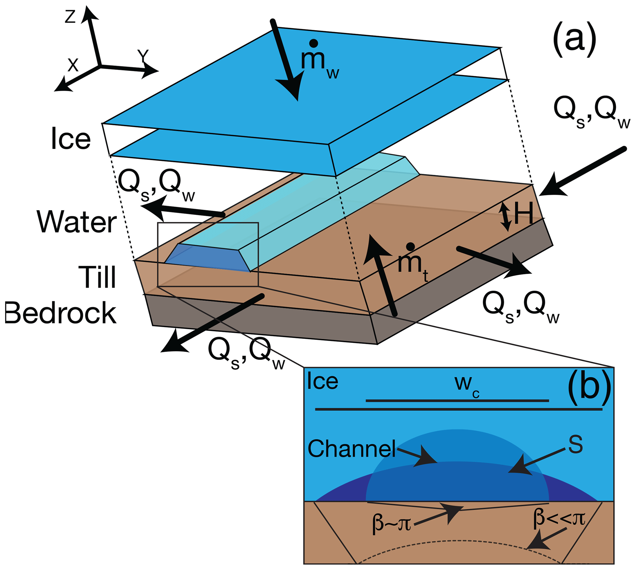
Figure 2Illustration of a model cell (a), detailing the layers of bedrock, till, water, and ice. Characteristics of the subglacial channel are noted as a polygon but shown in one dimension for clarity in (b) with the Hooke angle parameterization with two different channel shapes for different values of β (Eqs. 2, 9, and 10).
We calculate sediment mobilization in both supply- and transport-limited conditions. Divergence of the sediment flux is evaluated by approximating ∇⋅Qs with using a similar mobilization scheme as in Delaney et al. (2019)
is sediment mobilization across a width of the glacier bed w perpendicular to the water's flow direction. Note that w is not necessarily the channel width, but rather a representative width across the glacier bed over which sediment can be accessed by water flowing through the subglacial channel (Fig. 2). The channel width wc is used to calculate the width over which to apply the sediment discharge capacity and is discussed below in Eq. (9), which converts the hydraulic diameter Dh to channel width. Qsc is the sediment transport capacity or the maximum amount of sediment that could be transported under the given hydraulic conditions. l is a characteristic length scale for sediment mobilization, over which sediment mobilization adjusts to sediment transport conditions. σ is a sigmoidal function of H,
which enables a smooth transition from transport- to supply-limited transport in Eq. (6c). If H, the till thickness, is greater than 3Δσ, then the impact on sediment mobilization is negligible and the system is in a transport-limited regime. As H approaches Δσ, then σ(H) is close to 0 and sediment transport is in a supply-limited regime since no significant sediment mobilization takes place.
The condition in Eq. (6a) represents the case in which bedrock erosion exceeds sediment mobilization, and thus sediment transport exists in a transport-limited regime. The condition in Eq. (6b) impedes mobilization or deposition, therefore transporting sediment to the next cell when a till thickness is equal to Hlim, the value of which is chosen to be on the order of the maximal change in till height over the model run (∼10 cm). The condition in Eq. (6b) prevents unbounded sediment accumulation, as the model does not include physical processes to limit sediment deposition, such as reduced channel size and increased water velocity in response to the infill of sediment (Perolo et al., 2018). The condition in Eq. (6c) allows sediment mobilization to transition between transport- and supply-limited regimes, limiting sediment mobilization to the sediment production term, (see below), when H is small and thus minimal sediment is available for transport. With the conditions in Eq. (6a–c), we can calculate sediment transport in transport- and supply-limited regimes and pass sediment through the system.
We calculate sediment transport capacity Qsc using the total sediment transport relationship by Engelund and Hansen (1967),
where ρs (ρw) is the bulk density of the sediment (water), Dm is the mean sediment grain size, and τ represents the shear stress between the water and the channel bed.
The width of the channel floor wc, required to evaluate the surface over which sediment transport may occur, is given by
where, again, β is the Hooke angle controlling channel morphology (Sect. 2.1), and S is the cross-sectional area of the channel given by
Here, hydraulic diameter Dh is evaluated from Eq. (3).
We also determine the shear stress between water flowing through the channel and the sediment below in Eq. (8) through the Darcy–Weisbach relationship,
where is the water velocity. Water discharge Qw is calculated by the water flowing above a position in the glacier, and S, the cross-sectional area, is evaluated in Eq. (10). Other sediment transport relationships using shear stress could be exchanged by the model operator (e.g., Meyer-Peter and Müller, 1948). We have chosen the Engelund and Hansen (1967) formulation due to the representation of both suspended and bedload transport.
We assume that till armors the bed against erosion (e.g., Alley et al., 2003; Brinkerhoff et al., 2017; Delaney et al., 2019). In response, the source term, , is described as
where Hmax is a till height beyond which no further erosion, , may occur.
We use an empirical relationship with sliding velocity ub to describe bedrock erosion,
where kg is an erodibility constant and ler is an exponent, which varies between 0.66 and 3 (Herman et al., 2021). The sliding velocity, ub, is assumed to be related to basal shear stress (τb; Weertman, 1957) given the following relationship,
where B is a constant and we assume the exponent m is equal to 1.
We assume that τb is equal to driving stress (Cuffey and Paterson, 2010),
where ρi is the density of ice, h is the glacier thickness, and α is the surface slope of the glacier.
Note that alternative parameterizations of erosion or basal sliding can easily be exchanged for .
2.3 Spatial and temporal discretization as well as parameters
We describe the water and sediment routing and numerical implementation of the equations presented above.
2.3.1 Water and sediment routing and implementation
A routing scheme is implemented to (1) evaluate the hydraulic potential and thus the direction of the water flow and (2) transport sediment and water across the glacier bed to where it is expelled or deposited.
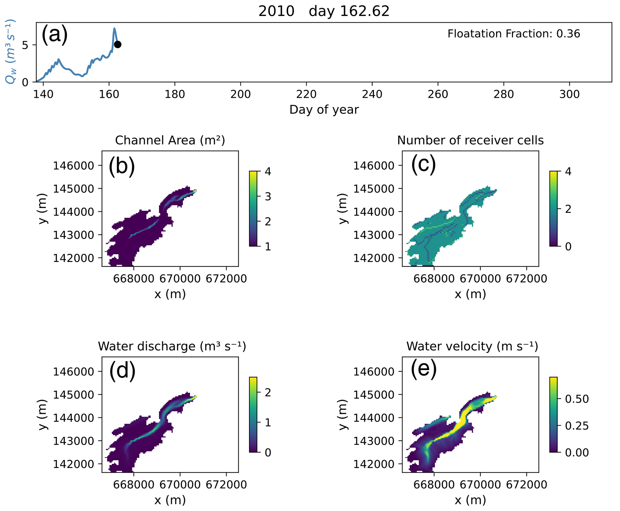
Figure 3Example of model parameters and variables for the snapshot of the Griesgletscher case in Sect. 3.2. (a) Glacier flotation fraction. (b) Channel cross-sectional area S with (d) distributed water discharge, (c) the number of receiver cells rt for a given cell, and (e) the water velocity.
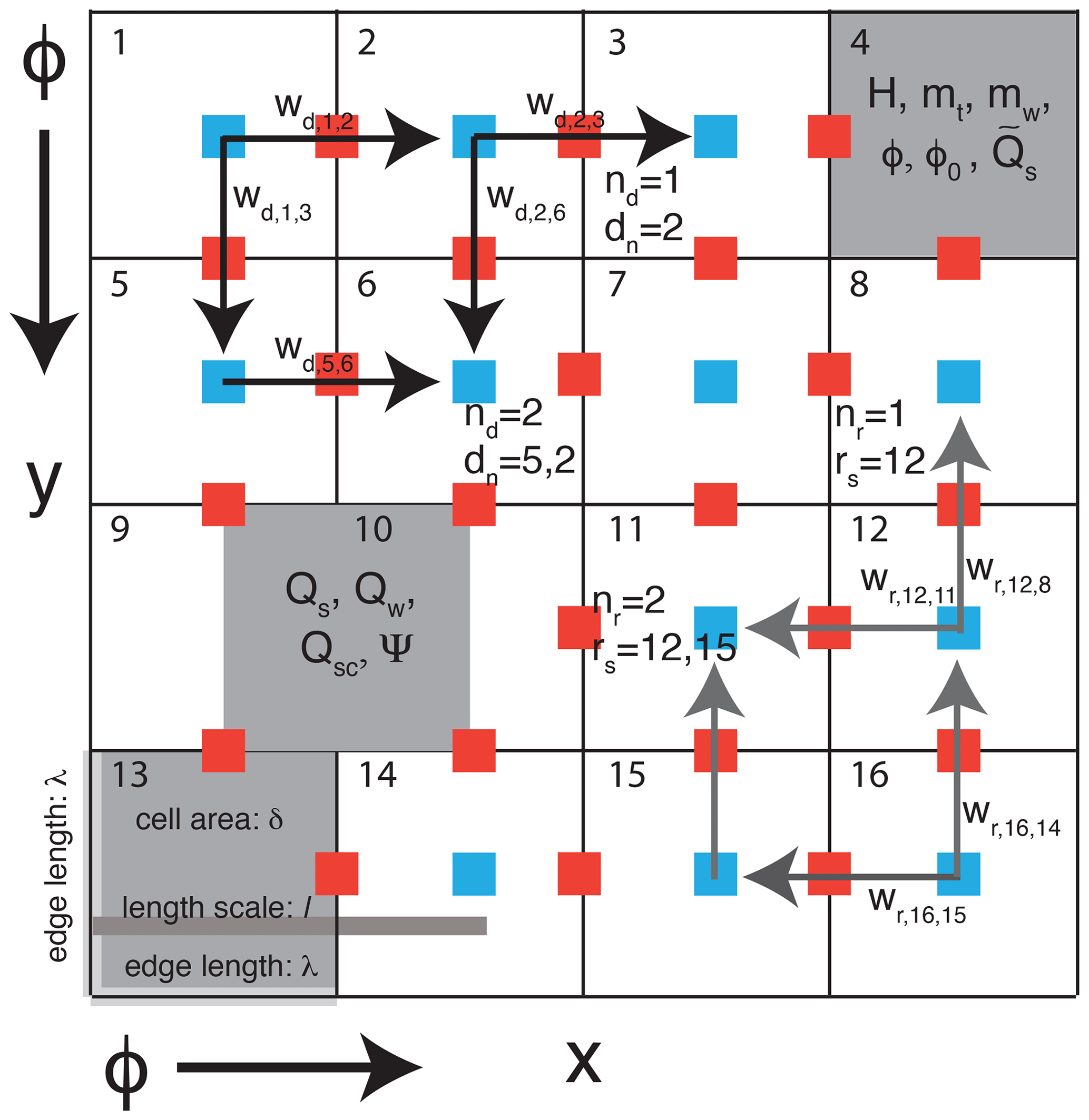
Figure 4Routing scheme on the grid. Solid lines represent cell boundaries, blue squares are cell centers, and red squares are cell edges. ϕ, the hydraulic potential, decreases in the direction of arrows so that water and sediment generally flow left to right and top to bottom. Edge length (λ) and cell area (δ) are shown. Cell numbers refer to identification in the stack (st). Select cells denote the weight of donors , number of donors nd, donor cells dn, number of receivers nr, and receiver cells rs. Variables and their respective locations on the grid are shown. Some red and blue squares have been removed in some cells for clarity.
To evaluate the hydraulic potential and thus the direction of the water and sediment flow across the glacier bed, we use a two-dimensional routing scheme (Quinn et al., 1991) to establish flow routing based on the steepest hydraulic potential. We implement this scheme in a similar fashion as Bovy et al. (2016), but on a regular grid with square cells, extending in x and y directions. Water and sediment fluxes can pass to the four surrounding cells sharing an edge as a result of the x and y components of the hydraulic gradient at a given point in time. This routing algorithm returns a stack (st; Table 3), which is a vector that contains information about the order of cells to perform the calculations, along with the number of cells flowing into a cell (donors; nd), the number of cells to which a single cell contributes (receivers; nr), and the weight or the percentage of hydraulic potential and water (or sediment) discharge directed from one cell to another (wd or wr), as determined by the hydraulic potential gradient between cells (Fig. 4).
We define the hydraulic potential, upon which the routing scheme is evaluated, at a cell i in the grid, ϕi, based upon the elevation of the glacier bed plus the ice thickness, following Shreve (1972):
where ff is the flotation fraction across the glacier, zs is the glacier surface, and zb is the glacier bed.
For the initial time step, the hydraulic potential ϕ is evaluated under the condition that ff=1. After the first time step, we assume that the flotation fraction will vary in response to changing hydraulic conditions, such as diurnal or seasonal water input (e.g., Iken and Bindschadler, 1986). In turn, to establish an average flotation fraction, ff, across the glacier bed for Eq. (16), we use
where the denominator represents the hydraulic potential at the overburden pressure of the glacier (ff=1 in Eq. 16), and i represents a cell in the grid.
ϕ0 represents the hydraulic potential evaluated from summing the gradient of the hydraulic potential, Ψ, in Eq. (1) up-glacier. ϕ0 at each cell i is evaluated as
Here, by evaluating Eq. (1), Ψi,j is established for receiver cell j of i, λ is the edge length of a cell on a regular grid, nr is the number of receivers that the cell i has, and is the proportion of the hydraulic potential fed by the upstream cell j to cell i. The operation is executed on a cell-by-cell basis, beginning with cells that have no receivers, such as those near the glacier terminus, and moving up the glacier using the inverted stack in st (Fig. 4).
Using the routing scheme above, we evaluate the water discharge from cell i, Qw,i, from melt upstream as
where nd is the number of donor cells for cell i, is the percentage of water flow from cell j to cell i, and is a prescribed meltwater source term in cell i. The operation begins with cells that have no donors (for instance at the top of the glacier) so that water accumulates down the glacier (Fig. 4). The amount of sediment leaving a cell i, Qs,i, is the flux into the cell plus the sediment mobilized in the cell, which is defined as
The first term is the flux of sediment into the cell i from donor cells j. The second term is sediment mobilization, , in cell i, which is computed by implementing Eq. (6a–c) as follows.
Qsc,j is the sediment transport capacity from cell j flowing to i, Qs,j is sediment discharge entering from cell j to cell i, l is a response length scale, and λ is edge length.
We evaluate the change in till height at a cell by implementing Eq. (5) as
where δ is the cell area (Fig. 4). The term Qs,i is the amount of sediment leaving the cell from Eq. (20), and the term is the sediment flux entering the cell from the donors.
2.3.2 Numerics and parameters
Spatial discretization on the regular grid must be substantially smaller than characteristic length scale, l, in Eqs. (6a–c) and (21). We then solve Eq. (22) to establish till height, H, for given initial and boundary conditions in response to till production, , and the divergence of the sediment discharge, Qs, using an explicit time integration scheme.
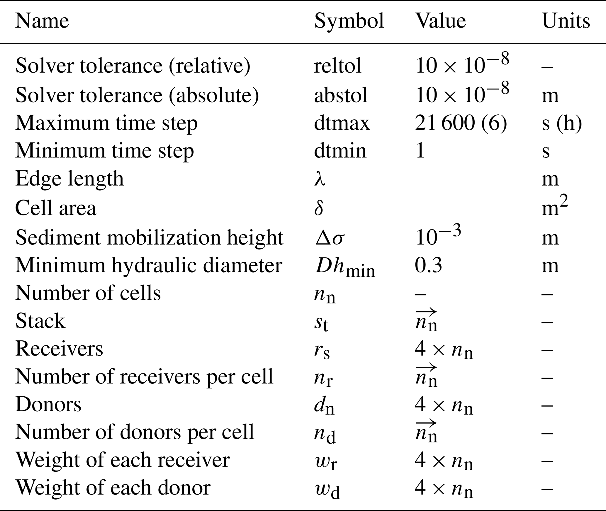
To discretize the problem in time, the model implements the VCABM solver (Hairer et al., 1992; Radhakrishnan and Hindmarsh, 1993) from the package DifferentialEquations.jl (Rackauckas and Nie, 2017) to evolve till layer height, H. This solver implements an adaptive time step and uses a linear Adams–Moulton multistep method that is well-suited to non-stiff problems, which is optimal because of the rapid fluctuations in sediment transport that can occur. We impose a maximum time step of 6 h to ensure that the model captures the response to diurnal variations in melt input. In practice, the solver commonly uses a time step of roughly 20 min, which varies depending on sediment transport conditions and solver tolerance. Longer time steps occur over periods with minimal glacier melt, and thus sediment transport ceases (i.e., winter months). Table 3 presents the numerical parameters used.
We execute the routing scheme based upon hydraulic conditions to the nearest 6 min to improve stability and fill closed basins in the hydraulic potential to maintain continuous sediment transport through the domain. Smaller solving tolerances increase the computational time due to (1) the increased accuracy of the solution and (2) the reassessment of flow fractions between the adjacent cells, which results in different routing configurations as the model converges.
We impose boundary conditions on the edge cells so no sediment or water enters the domain. At outlet cells, water discharge leaves the domain, as does a flux of sediment, based on sediment transport conditions. In other applications, boundary conditions could also be set to represent processes such as hillslope erosion or glacial lakes, which route sediment or water to the subglacial environment (e.g., Andersen et al., 2015). At the outlet cells, we assume that the hydraulic potential has no ice overburden pressure.
Evolving Eq. (5) requires an initial till height, H0, chosen by the model user. This initial till height represents material from bedrock erosion created prior to the model initialization. We apply a “spin-up” procedure to create a reasonable relationship between the amount of fluvial sediment transport and bedrock erosion.
New versions of the code are tested against reference cases to ensure consistency. Additionally, in each test, we ensure mass conservation by verifying that the amount of sediment leaving the system through fluvial transport is consistent with the till height change and erosion occurring under the simulated glacier.
We use two case studies to highlight model viability under increasingly complex situations. First, we apply the model to a synthetic alpine glacier topography with a synthetic hydrologic forcing, based on the Subglacial Hydrology Model Intercomparison Project (SHMIP; de Fleurian et al., 2018), to illustrate the model's performance in a simplistic scenario. We then apply the model to the topography, sediment, and water discharge at Griesgletscher in the Swiss Alps. We demonstrate its proficiency by comparing the calculated sediment transport output with measured data (Delaney et al., 2018a). We also identify important factors controlling subglacial sediment discharge in these simulations.
3.1 Synthetic alpine case
3.1.1 Experiment design
We run simulations using a synthetic alpine glacier geometry, along with seasonally and diurnally varying hydrological forcing from the SHMIP experiments (de Fleurian et al., 2018). The domain is 6000 m on one axis and 1080 m on the other (Fig. 7). The resulting geometry approximates the Bench Glacier in Alaska. The U-shaped bed and variable ice thickness mean that variable hydrologic gradients will occur perpendicular to the flow, and thus water and sediment are routed across multiple cells.
To represent a hydrological environment that varies both seasonally and diurnally, we implement a simple spatially distributed melt model, as in SHMIP (de Fleurian et al., 2018):
where Mf=0.01 m ∘C−1 d−1 is a melt factor, and is the basal melt rate. T(zs) is air temperature T (∘C) at elevation zs, defined as
where Aa and Ad are the annual and diurnal amplitudes in temperature, respectively, ΔT is a temperature offset that is adjusted to control the meltwater input, sday represents the number of seconds in 1 d, syear is the number of seconds in a year, and ∘C m−1 is the air temperature lapse rate (de Fleurian et al., 2018). In this case, we route water directly to the subglacial system at the location where the melt occurs, omitting moulins or crevasses that concentrate meltwater delivery to the bed, for instance.
We run the model for 10 years with a steady climate; we then apply a linear temperature increase of 0.5 ∘C a−1 for 10 years followed by 10 years of steady temperature at the maximal ΔT. We implement this dramatic warming to capture the model's ability to represent different climatic conditions. The model is initiated with 5 cm of till across the bed. To spin up the model, we apply the initial year of hydrological forcing for 5 years to limit computational time. In other applications, the spin-up could be maintained until the annual change in till height was well below commonly accepted glacier erosion rates (Hallet et al., 1996).
3.1.2 Model outputs and findings
The simulations show that over seasonal timescales, sediment discharge increases at the onset of melt and decreases shortly thereafter, but prior to the maximum amount of water discharge that occurs at the peak of each melt season (Fig. 5). Maximum and average quantities of daily sediment discharge decrease until the very end of the melt season, when sediment discharge increases very slightly again (Figs. 5 and 6b, d, f). This slight increase occurs when water stops flowing during the night, allowing sediment from bedrock erosion to briefly accumulate in the channels from bedrock erosion. Increased sediment discharge produced by the model at the beginning of the melt season results from greater sediment availability following the growth of the till layer over the winter months when the small amount of melt prevents substantial transport of sediment. In fact, similar increases in sediment discharge have been observed in alpine glaciers at the onset of melt each season (Figs. 5b and 6b, d, f) (Willis et al., 1996; Swift et al., 2005; Riihimaki et al., 2005; Delaney et al., 2018b) and are reproduced in the one-dimensional version of the model in Delaney et al. (2019).
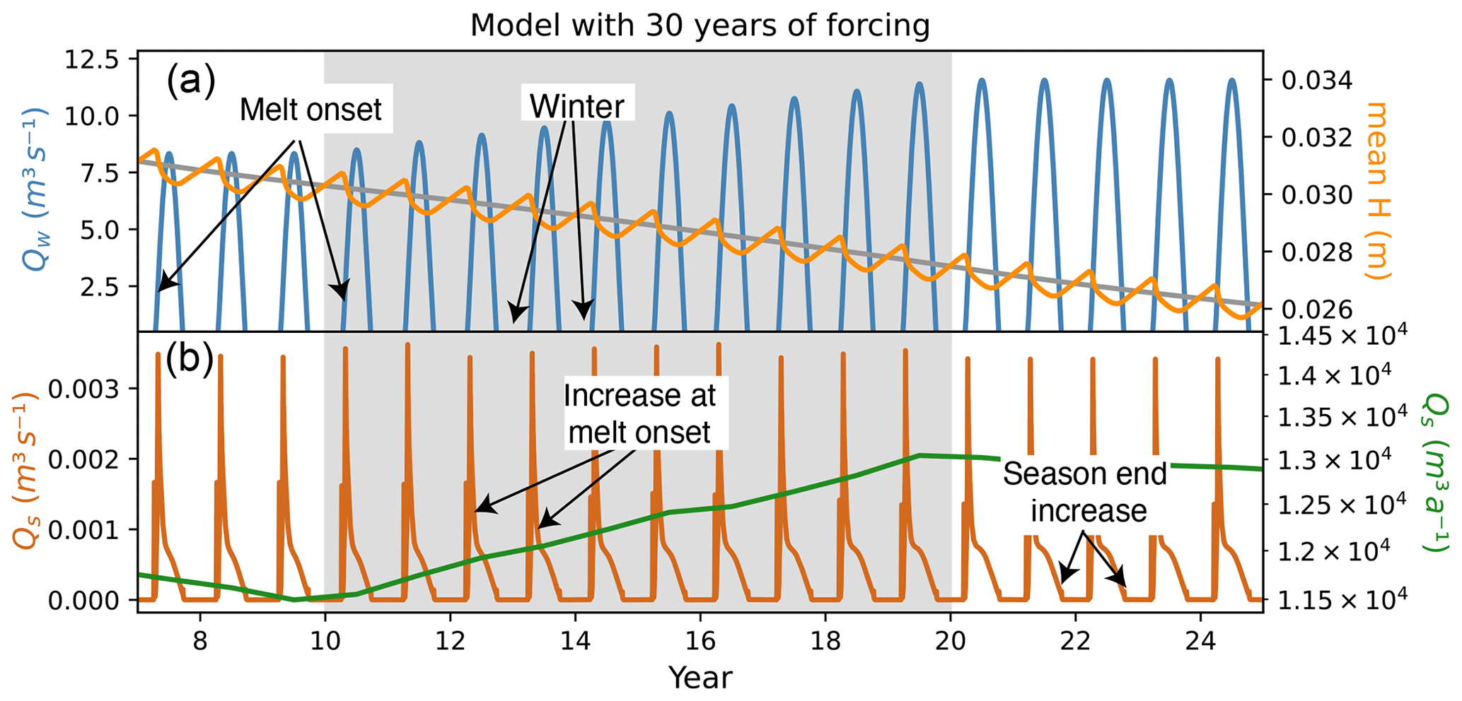
Figure 5Model output from a synthetic alpine topography and forcing over a 30-year run with diurnal and seasonal variations in melt input as daily mean values. The gray box represents a time period of increasing glacier melt. (a) Daily averaged seasonally varying water discharge (Qw) increases from year 10 to 20, while till height (H) decreases throughout the model run, with seasonal increases in the absence of glacier melt. (b) Daily averaged sediment discharge in brown shows strong seasonal variability. Annual sediment discharge (green) increases with increasing melt, with the highest sediment discharge occurring in year 19 when glacier melt is greatest. During stable climate temperatures before and after the increase in temperature, annual sediment discharge generally decreases. However, following the melt, Qs stabilizes at a higher level due to the increased area over which sediment is transported.
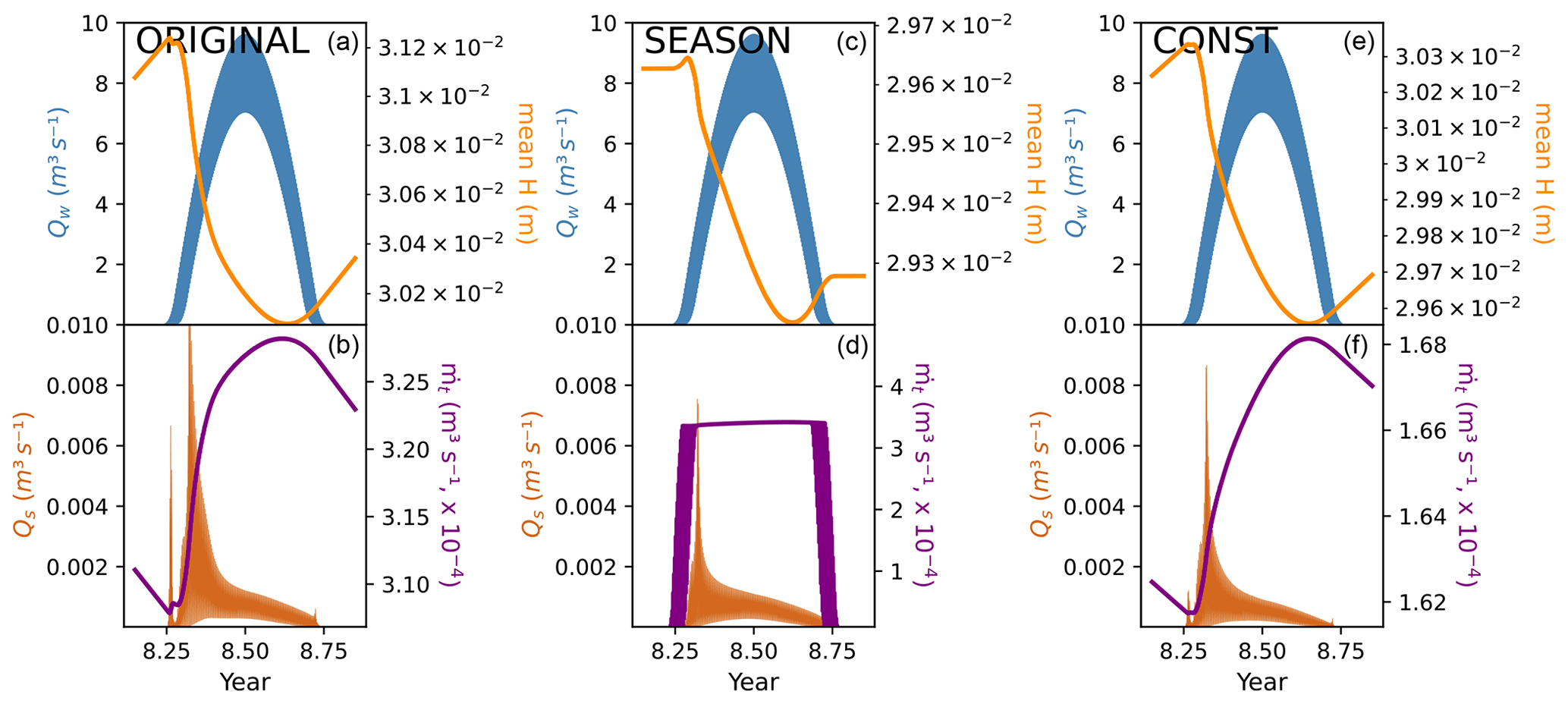
Figure 6Annual response to different till production patterns across the synthetic glacier case studies. (a, b) Conventional model setup in which sediment is produced year-round, ORIGINAL. (c, d) Setup equivalent to the previous setup, except sediment is produced only in summer months when water is present at the glacier bed, SEASON. Note that till height remains constant on the edges of the plot over the winter months. (e, f) Steady erosion of 2 mm a−1 across the entire synthetic glacier, with no spatial or temporal variability in sediment production, CONST. Data are plotted at a 6 h interval so that daily maximums and minimums are visible.
Over the course of the simulation, the mean till height across the glacier generally decreases throughout the model run, although there are small increases in till height during the winter months without sediment transport and larger decreases in till height during the time periods with substantial melt (Figs. 5a and 6a, c, e). Exhaustion of sediment is evident in the middle of the glacier where much of the water flows as a result of the spin-up procedure prior to the model initialization (Fig. 7e and f). Note that the decreasing till height through the model run results from sediment mobilization on the margins of the glacier, where increased water flow occurs more often in a warmer climate. During the climate warming from years 10–20, sediment discharge from the glacier increases due to greater melt and water discharge on the upper reaches of the glacier. This results in increased sediment transport at higher elevations on the glacier, where sediment could persist in a cooler climate (Fig. 7e and f). Following the stabilization of the climate at year 20, sediment discharge remains elevated compared to the cooler climate because sediment transport occurs over a larger region of the glacier bed (Fig. 5b).
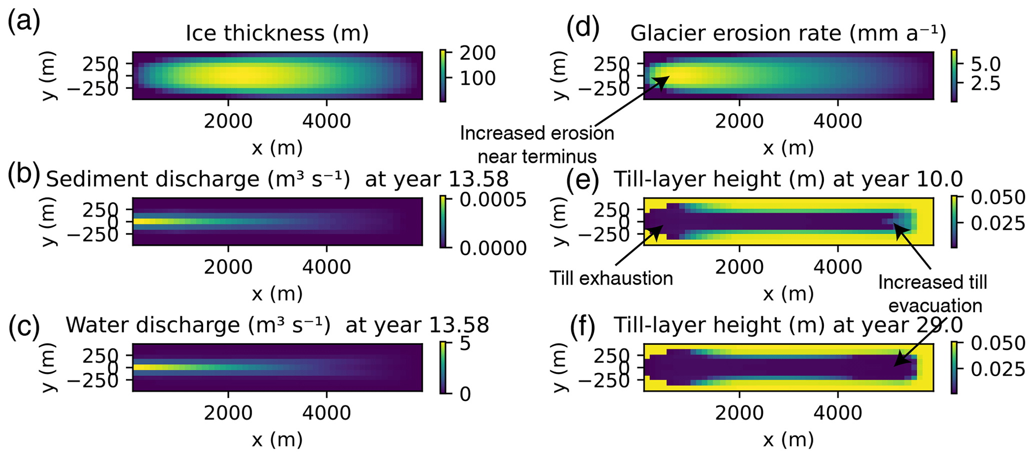
Figure 7Spatial view of synthetic case (Sect. 3.1). Spatially distributed (a) ice thickness (h), (b) sediment discharge (Qs), (c) water discharge (Qw), (d) glacier erosion rate (), (e) till layer height (H) at year 10 prior to warming, and (f) till layer height (H) at year 29 near the end of the model run. Spatial differences in the distribution of water and sediment discharge in panels (e) and (f) result from the depletion of subglacial till beneath the glacier. We have included an animation of this figure in the Video supplement.
In the model, bedrock erosion relies only on driving stress and till thickness. Sliding and bedrock erosion did not vary seasonally with increased subglacial water discharge (Fig. 5a). This causes sediment to accumulate during the winter months, which subsequently provides ample material for transport when melting increases in the spring. To test the effects of spatially variable erosion and the role of hydrology, we present two additional cases to supplement the synthetic alpine glacier case above, named ORIGINAL. An additional synthetic case, SEASON, simulates bedrock erosion by only allowing sliding, and thus erosion, during the summer months (e.g., Iken and Bindschadler, 1986; Herman et al., 2011); the same erosional relationship is applied as that in Sect. 3.1 (Eqs. 13 and 12). In the SEASON case, however, erosion occurs only when the amount of water input substantially exceeds the background basal melt input rate that is present in the winter. This case captures the seasonal variations in bedrock erosion (Ugelvig et al., 2018). In another additional case, CONST, bedrock erosion remains constant over the entirety of the glacier at a rate of 2 mm a−1, independent of the spatially varying glacier sliding velocity of the other cases (Fig. 7).
The ORIGINAL case discharges over 11 620 m3 of sediment per year, while the SEASON case discharges only 60 % of that value due to the absence of bedrock erosion during the winter months. The CONST case discharged 7320 m3 of sediment over the year or 63 % of the ORIGINAL case. The quantity of sediment discharge in the CONST case results in a catchment-scaled height change in the till layer of approximately 1.1 mm a−1 due to decreased erosion efficiency with till height instead of the prescribed bedrock erosion rate of 2 mm a−1 (Eq. 12). Additionally, the spatial disparity of where sediment is produced at the glacier bed compared to the location of sediment transport further reduces the catchment-scaled height change (Fig. 7e and f).
In each of the three synthetic cases, sediment discharge increases at the onset of melt and substantially decreases by the end of the melt season due to sediment exhaustion (Fig. 7). In ORIGINAL (Fig. 6a and b), greater sediment discharge occurs compared to the alternate cases (SEASON and CONST). The increased sediment discharge in ORIGINAL results from (1) the winter periods without melt over which bedrock erosion adds more sediment to the layer in the absence of sediment transport and (2) bedrock erosion that occurs low on the glacier where much of the sediment transport occurs (Fig. 7d). By contrast, in the CONST case, a steady amount of erosion occurs across the entire glacier bed. The peak sediment discharge in CONST (Fig. 6e and f) occurs slightly earlier in the season compared to the ORIGINAL and SEASON cases due to the increased amounts of sediment below the glacier's lower portions.
3.2 Griesgletscher
3.2.1 Experiment design
We also run simulations of Griesgletscher in the Swiss Alps using topographic data from Delaney et al. (2019). Here, we run the model from 2009–2017, with the modeled water discharge time series from Delaney et al. (2018a). Subglacial sediment discharge from the glacier is determined over four different time periods (2011–2013, 2013–2014, 2014–2015, 2015–2016) by differencing the bathymetry maps collected through this period and considering proglacial erosion quantities (Delaney et al., 2018a, 2019). To estimate surface melt across the glacier with respect to elevation, we use
Here, γ is the mass balance gradient, represents the glacier's lowest elevation, and represents the melt rate at the glacier's lowest extent. was evaluated numerically at each water discharge value using the hypsometry of the glacier.
We apply a parameter search over a range of values of sediment grain size (Dm, representing a primary control on fluvial transport of subglacial sediment), sliding rate factor (B, representing a control on bedrock erosion), and the initial till height condition (H0, representing the effects of existing quantities of sediment below the glacier). A total of 100 simulations were run with randomly selected parameters from a uniform distribution. No spin-up was applied in this case to establish an initial condition because of the wide range of H0 values explored.
The wall time for a single model run averaged 8.9 h, and each run for a parameter set was executed on a single CPU. Instead of applying the mean flotation fraction across the glacier, as done in the synthetic cases, the maximum value was applied with an upper limit of 1.
We consider model outputs resulting in a perfect rank correlation across the four data collection periods and have errors less than the 131 000 m3 of sediment that was expelled from the glacier over this period (Delaney et al., 2018a, 2019). For the example presented below, we show the simulation with the lowest absolute error between the model output and the sediment transport data.
3.2.2 Model outputs and findings
The parameter search yields an optimum grain size parameter Dm of 2 cm, sliding parameter B of MPa m s−1, and initial till height H0 of 2.5 mm (see red stars, Fig. 8a–c). The model's ability to reproduce the quantities of sediment in the validation data largely depends on the grain size parameter, Dm, shown by Fig. 8a. Compared to Dm, the sliding parameters (B) and initial condition parameters (H0) have a reduced influence in representing the measured data, given that similar values of B and H0 can produce largely different model outputs in the context of Dm (Fig. 8a–c).
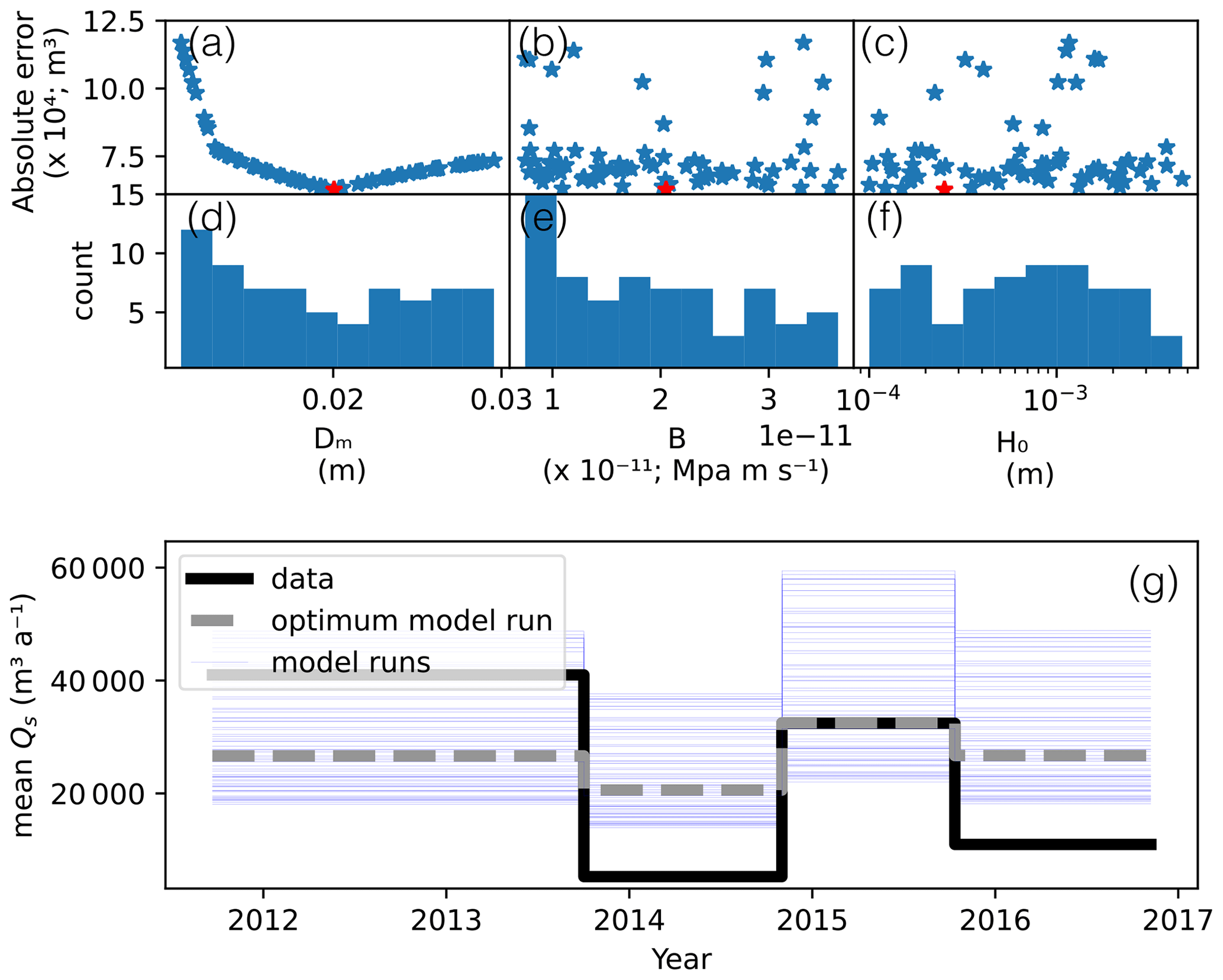
Figure 8Results of the parameter search (a–c), the frequency of parameter values that produced a rank correlation of 1 (d–f), and average sediment flux from the model run amongst the parameter combinations over the time periods (g) in the Griesgletscher case. Red stars represent the optimum parameter combination with an absolute error of roughly 62 600 m3. Blue lines represent all model outputs, while the gray line represents the optimum parameter combination.
The optimized parameter combination, along with other parameter combinations, reproduces the interannual variability in sediment discharge from the Griesgletscher (Fig. 8g). The absolute error between the optimum model run and the measured data is roughly 62 600 m3 of sediment. The error is slightly less than half of the 131 300 m3 total sediment discharged from the Griesgletscher over this time period from 2011 to 2016 (Delaney et al., 2018a). In fact, the model runs capture the third period from late 2014 to late 2015 well. However, the runs systematically overestimate the second and fourth periods and generally underestimate the high-sediment-discharge period from late 2011 until late 2013 (Fig. 8g).
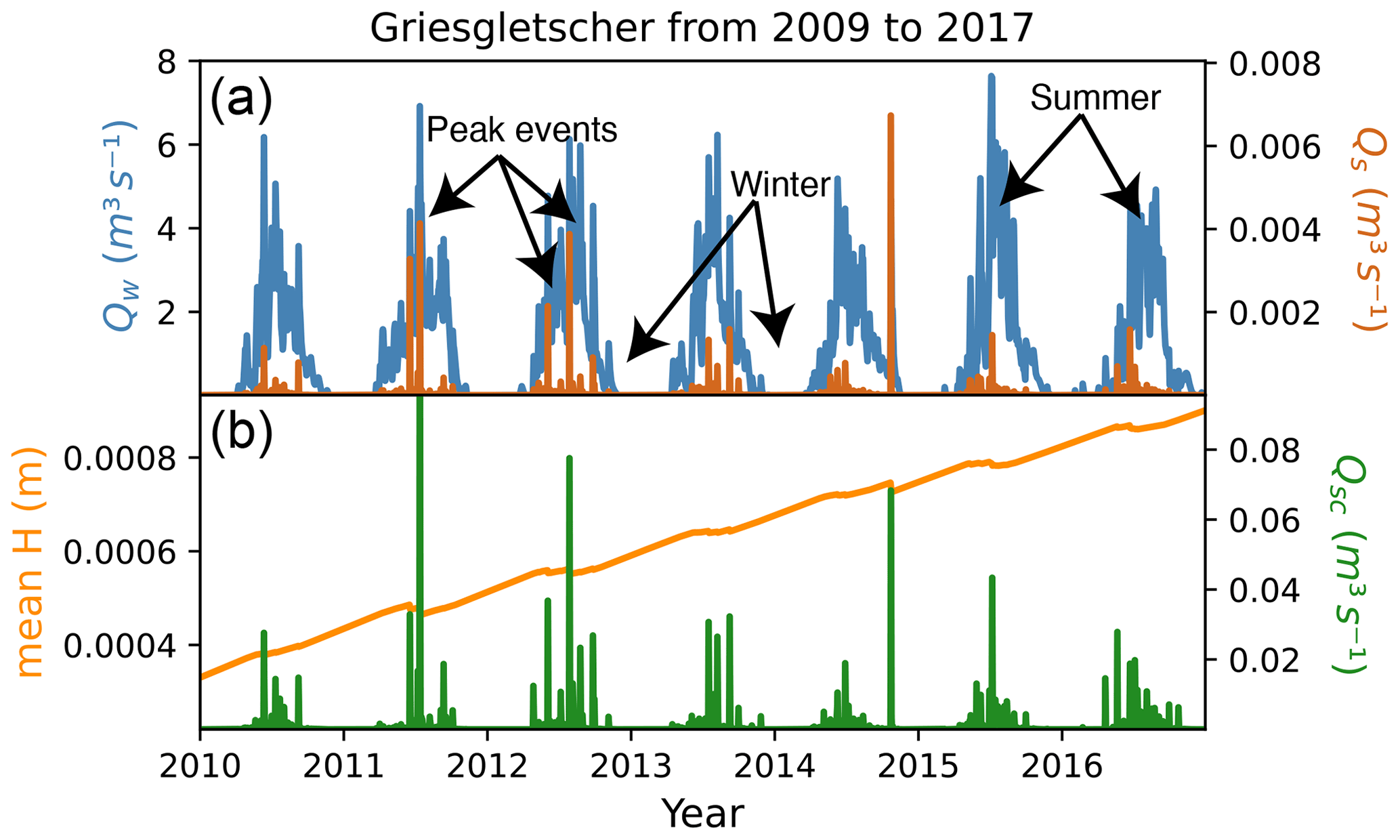
Figure 9Time series of model output from optimum parameter combinations. (a) Daily averaged water discharge, an input modeled for Griesgletscher, Switzerland, in Delaney et al. (2018b), and sediment discharge, the output of the model, from Griesgletscher beginning in 2010. (b) Daily averaged sediment transport capacity and average till height. Note that sediment discharge capacity is roughly 1 order of magnitude larger than sediment transport discharge. Additionally, the increasing trend in till height, H, through this model run shows that sediment is produced at a greater rate than it is transported from the glacier bed.
The best-performing model run shows strong temporal variability in sediment discharge (Fig. 9a). Some of the peaks in sediment discharge occur during the short periodic increases in water discharge. Yet the greatest sediment discharge values do not necessarily occur at the highest water discharge values (Figs. 9a and 10a). Despite the strong dependence on grain size and fluvial transport of sediment in the parameter search (Fig. 8a), the modeled sediment transport capacity Qsc still remains roughly an order of magnitude higher than the calculated sediment discharge Qs (Fig. 9a and b). The steep section of the glacier (Fig. 11c) experiences sediment depletion over the model run, as do several patches of the glacier bed near the overdeepening and high on the glacier (lower left of panels in Fig. 11c and d). On some parts of the upper glacier, the calculated bedrock erosion grows the till layer beyond the initial condition in the absence of substantial sediment transport.
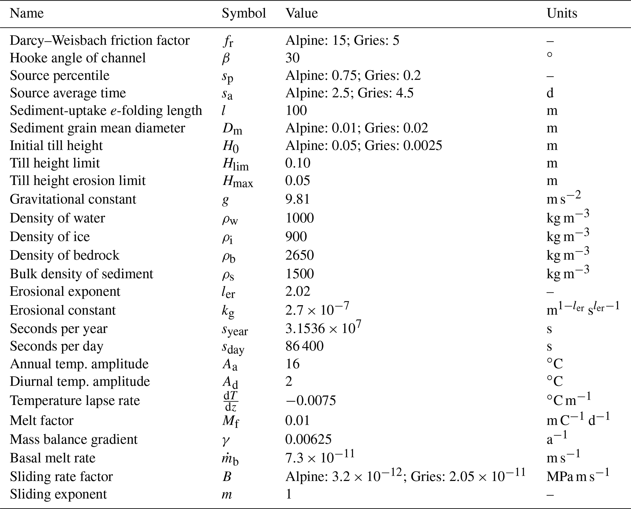
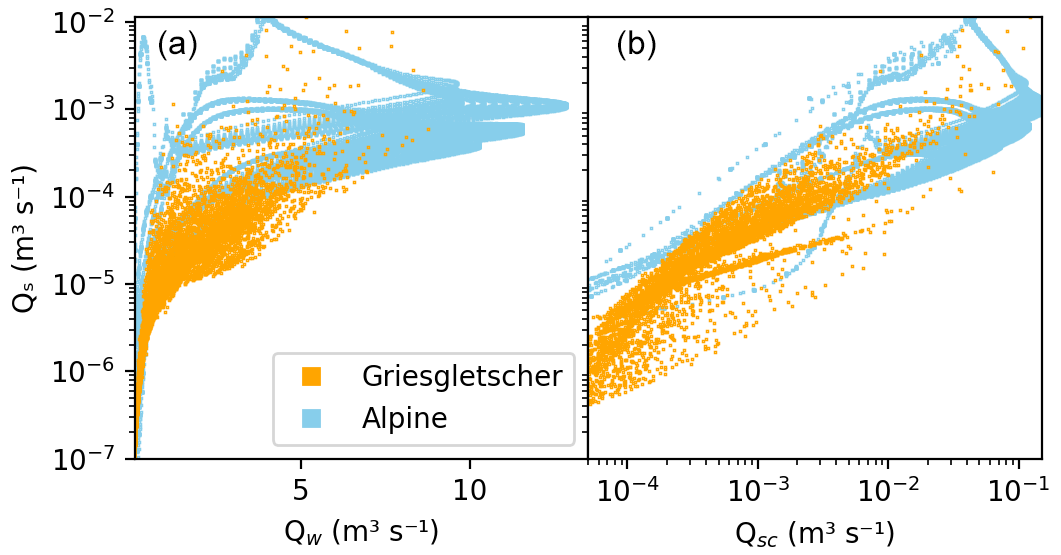
Figure 10Model outputs of sediment discharge from the glacier compared to water discharge (a) and sediment transport capacity (b).
The range of values for B, the sliding parameter, in the parameter search results in mean sliding velocities across the glacier between 14 and 70 m a−1 (Eq. 14). The optimum run in the parameter search results in an average sliding velocity of 39 m a−1. We note that smaller sliding velocities could result in equivalent amounts of erosion if the parameters kg and ler in Eq. (13) are increased. The model reveals that the relatively large velocities needed to produce adequate amounts of erosion occur in part because sediment production in the model is limited to the narrow patches of the glacier bed where minimal till persists and bedrock erosion may occur. As a result, the model requires more sliding to produce the equivalent amount of sediment with more till at the bed, even though the sliding and erosion parameters applied here are within a reasonable range (Fig. 11c and d).
The lack of observations of the spatial distribution of subglacial sediment makes selecting an initial value of H, the height of the dill layer, difficult. The slow rate of basal erosion suggests that an equilibrium between fluvial sediment transport and bedrock erosion will likely take centuries to attain if such an equilibrium could even exist in light of the variability in climatic, and thus glacier, conditions. Should an equilibrium eventually be present (e.g., Herman et al., 2018; Delaney and Adhikari, 2020), it is probably beyond a feasible computational time for this model, given its processing speeds.
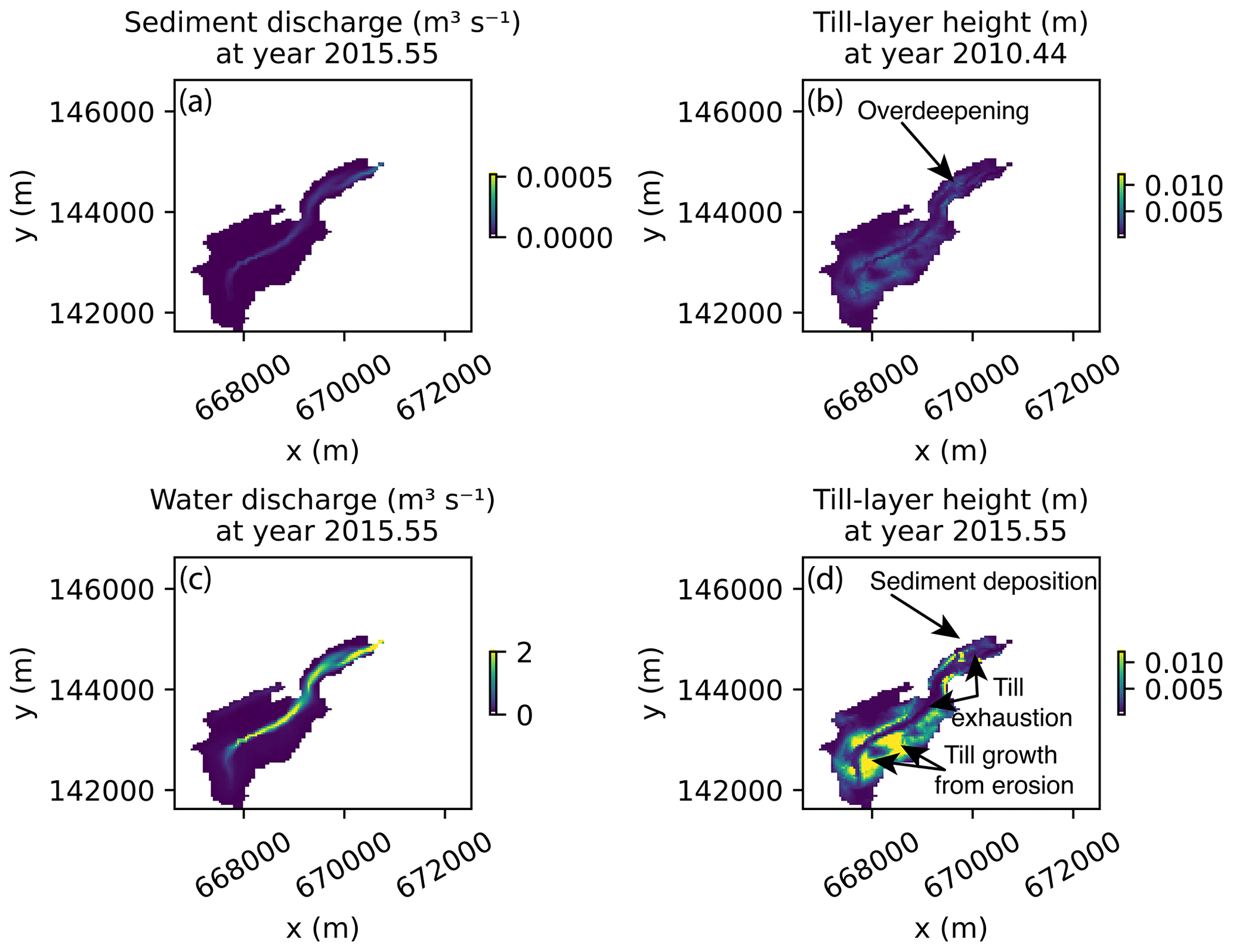
Figure 11Spatial view of characteristics from the Griesgletscher model run (see Fig. 1 images). (a) Subglacial sediment transport is concentrated in a narrow part of the bed, (b) and water discharge is also highly variable across the bed. Till layer height changes substantially from the beginning of the model run (c) to the end of the model run (d). We identify the overdeepening near the glacier terminus as well as a steep section connecting the upper and lower glacier. Over this time, till exhaustion in regions of high water flow is visible, while other regions of the glacier bed experiencing sediment deposition and till growth from glacier erosion can be identified. We have included an animation of this figure in the Video supplement.
SUGSET_2D also contains 20 parameters (Tables 2 and 3). In the available literature, some of these parameters have been partially constrained using inverse methods (Brinkerhoff et al., 2016) as well as detailed modeling and measurements (e.g., Chen et al., 2018; Covington et al., 2020; Pohle et al., 2022). However, many are poorly constrained.
For instance, we limit the thickness at which the till layer must stop accumulating sediment (Eq. 6b, Hlim) due to the changes in the hydraulic potential caused by channel infill of sediment. We assume that this value is on the order of tens of centimeters (Table 2) based upon available observations of sediment deposition and glacier uplift (Perolo et al., 2018). While the impact of a till layer on bedrock abrasion remains uncertain, we expect that sediment of a certain thickness will armor the bed, preventing erosion (Alley et al., 2003). In turn, we limit erosion with till thickness to a threshold (5 cm) of the same order as Hlim to improve computational time. Due to the difficulty of making direct observations at glacier beds, only one study, to our knowledge, has quantified till thickness at a single point below a glacier (Truffer et al., 2000). The initial till height, H0, in the model must therefore be chosen thoughtfully because the system will remain impacted by this boundary condition throughout the model run. Furthermore, the model does not consider the interactions between fluvial sediment transport, debris concentrations in subglacial ice, and bedrock erosion, which may be important for subglacial sediment transport (e.g., Ugelvig et al., 2018).
The routing method we use assumes that the water flow direction is in response to the Shreve potential (Sect. 2.3.1). Therefore, it does not explicitly simulate the evolution of efficient and inefficient subglacial drainage systems over the course of the season or the inheritance of existing subglacial canals or channels (Fig. 3; e.g., Werder et al., 2013; Zechmann et al., 2021). In addition, a response time of the subglacial channel is chosen prior to simulations; this could be compared to a more sophisticated, but computationally more expensive, representation of processes in an R-channel model (e.g., Röthlisberger, 1972). Lastly, we have chosen a single friction factor fr for the entirety of the run. This factor can vary in time (Pohle et al., 2022) and can be impacted by other factors such as sediment grain size or bedrock along the channel bed.
Results of the one-dimensional model (SUGSET; Delaney et al., 2019) and the two-dimensional model, SUGSET_2D, highlight the importance of simulating the spatial heterogeneities in bedrock erosion, sediment availability, and sediment transport capacity. In the one-dimensional version of SUGSET, water can access sediment from the till layer across the entire glacier width, perpendicular to the glacier flow line. In SUGSET_2D, however, sediment access and transport are not averaged over the glacier width. Rather, by considering the spatial distribution in water discharge and sediment availability laterally below a glacier, the model evaluates where heterogeneities may persist and how these heterogeneities will impact subglacial sediment dynamics (Figs. 7 and 11).
In SUGSET_2D, large diurnal increases in sediment discharge occur near peak daily melt because the area of flowing water expands under the glacier (Fig. 6b, d, and f). As a result, increased sediment transport can occur in regions of the glacier bed with substantial sediment when hydraulic conditions permit; that patch of bed is abandoned when water is routed to another part of the glacier bed (Video supplement). This allows sediment to be stored in these regions of the bed until the hydraulic conditions return and renew the increase in sediment transport. Such processes cannot be represented in a one-dimensional model, wherein the entire width of the glacier evolves together (Figs. 5b and 6b, d, f; Video supplement).
When we compare the model runs across the space of three parameters, Dm, B, and H0, to sediment discharge data from Griesgletscher in the Swiss Alps (Sect. 3.2) we find that the model has a limited ability to capture the large sediment discharge from the first time period (2011–2013). The reduced sediment discharge in the second and fourth time periods, 2013–2014 and 2015–2016, indicates that the model does not adequately represent the processes that are responsible for the measured increases in sediment transport in these time periods (Fig. 8). Such processes may include variable flow routing following channel shape (Eqs. 1 and 2) or flotation fraction (Eq. 16). Additional processes may also be omitted due to model inputs. For instance, the evolving surface topography, not considered here, may cause alternative flow paths below the glacier (Fischer et al., 2005) and exposes new patches of the glacier bed to sediment transport or the relocation of channels (e.g., Zechmann et al., 2021). Furthermore, glacier sliding remains constant over the model run, so the results do not explicitly account for seasonal or interannual variability in bedrock erosion (e.g., Herman et al., 2015; Ugelvig et al., 2018); however, temporal variations in bedrock erosion are calculated through changing till thickness (Eq. 12 and Fig. 9).
Model performance at Griesgletscher depends greatly on sediment grain size compared to other parameters such as the initial till condition or bedrock erosion (Fig. 8c and d). Grain size is a strong control on sediment discharge in SUGSET_2D because it modulates sediment mobilization in patches of the bed only occasionally accessed by subglacial flow during the melt season – after sediment has been largely evacuated from the main channel (Fig. 11). This process cannot be fully represented in a one-dimensional model. This is especially so because the main flow paths under the glacier can be evacuated of sediment (Fig. 11c and d). Thus, these flow paths contribute to the catchment's sediment discharge only through the new production of sediment through erosion (Eq. 12). However, the dependence on grain size suggests that the connectivity between subglacial channels and distal sediment patches is a strong control on sediment discharge from the subglacial system. While this seems to be an important process on the relatively small and shallow Griesgletscher alpine glacier (Delaney et al., 2018a), sediment discharge on other, potentially steeper, glaciers may respond more strongly to processes such as bedrock erosion (Herman et al., 2015). The connectivity between the main channels and distal sources of sediment occurs through the fluvial transport capacity of sediments here, but this connectivity may also be influenced through processes not considered in the model, such as till deformation (e.g., Damsgaard et al., 2020) or sediment sorting (e.g., Bacchi et al., 2014).
Lastly, the model demonstrates the complex nature of subglacial sediment transport and the transitions between supply- and transport-limited regimes. Equivalent values of water input and sediment transport capacity below the glacier result in simulated sediment discharges that vary over orders of magnitude (Fig. 10). In turn, using solely the water discharge or sediment transport capacity (e.g., Eq. 8) fails to consider the changes to sediment availability caused by sediment transport, especially when changes to sediment storage can take place over seasonal to decadal timescales.
A two-dimensional subglacial sediment transport model, SUGSET_2D, evolves a till layer in response to changing subglacial hydraulic conditions. The model represents sediment transport in supply- and transport-limited regimes, and sediment and water are routed across the bed in response to changing hydraulic conditions in two horizontal dimensions. The till layer is supplied with sediment either from bedrock erosion or by existing sediment, represented by the initial condition. Model cases utilize geometries and hydrological forcings from a synthetic case and Griesgletscher, an alpine glacier in the Swiss Alps.
The interdependence of a large number of parameters and their interactions with one another – for instance, sliding and erosion (Eqs. 12 to 15) – at the very least point to the complexity of sediment transport in the subglacial system. Furthermore, the model's limited representation of the magnitude of interannual variability in the Griesgletscher simulation, from 2011 to 2017, points to processes not completely represented in this application of the model. This misfit could come from poorly constrained parameters and external factors, such as model inputs that may limit the model's accurate representation of sediment discharge observations. These include interannual variability of glacier velocity and thus bedrock erosion, changing glacier topography that routes water to different patches of the glacier bed over time, and routing of water to the glacier bed.
Additional insights into subglacial erosion and sediment transport processes over decadal timescales can be gained from more sophisticated parameterizations of bedrock erosion and subglacial hydrology. Even so, the foundational processes of the model presented here should be considered when examining subglacial sediment transport processes at seasonal to decadal scales. These processes include (1) fluvial transport of subglacial sediment across a glacier's bed in two dimensions in supply- and transport-limited regimes, (2) spatially distributed bedrock erosion or sediment production, and (3) variable water routing in response to changing melt and hydraulic conditions. It is our hope that the model will be applied in the context of field observations to evaluate and isolate subglacial processes controlling sediment discharge from glaciers as they change.
The model is available at https://doi.org/10.5281/zenodo.7975219 (Delaney et al., 2023).
Videos of the model's application to Griesgletscher are available at https://doi.org/10.5281/zenodo.7975219 (Delaney et al., 2023).
ID designed the study, developed the model, ran the cases, and led writing the paper. LA assisted with writing the paper and provided key advice on designing and troubleshooting the model. FH provided guidance with implementing and designing the model and preparing the paper.
The contact author has declared that none of the authors has any competing interests.
Publisher's note: Copernicus Publications remains neutral with regard to jurisdictional claims in published maps and institutional affiliations.
We thank Jean Braun, Benoit Bovy, Fien De Doncker, Guillaume Jouvet, Stuart N. Lane, Gunther Prasicek, and Mauro Werder for fruitful discussions and insightful comments. We are also grateful to Grégoire Mariéthoz and the Scientific Computing and Research Support Unit at Université de Lausanne for providing computing resources. Gabrielle Vance provided comments on the writing. Ian Delaney was funded in part by SNF project no. PZ00P2_202024. The editor, Frances E. G. Butcher, along with Irina Overeem, Stefan Hergarten, and two anonymous reviewers, provided thoughtful and constructive comments that greatly improved this paper.
This research has been supported by the Swiss National Science Foundation (grant no. PZ00P2_202024).
This paper was edited by Frances E. G. Butcher and reviewed by Irina Overeem, Stefan Hergarten, and two anonymous referees.
Alley, R. B., Cuffey, K. M., Evenson, E. B., Strasser, J. C., Lawson, D. E., and Larson, G. J.: How glaciers entrain and transport basal sediment: physical constraints, Quaternary Sci. Rev., 16, 1017–1038, https://doi.org/10.1016/S0277-3791(97)00034-6, 1997. a, b, c
Alley, R. B., Lawson, D. E., Larson, G. J., Evenson, E. B., and Baker, G. S.: Stabilizing feedbacks in glacier-bed erosion, Nature, 424, 758–760, https://doi.org/10.1038/nature01839, 2003. a, b
Andersen, J. L., Egholm, D. L., Knudsen, M. F., Jansen, J. D., and Nielsen, S. B.: The periglacial engine of mountain erosion – Part 1: Rates of frost cracking and frost creep, Earth Surf. Dynam., 3, 447–462, https://doi.org/10.5194/esurf-3-447-2015, 2015. a
Bacchi, V., Recking, A., Eckert, N., Frey, P., Piton, G., and Naaim, M.: The effects of kinetic sorting on sediment mobility on steep slopes, Earth Surf. Proc. Land., 39, 1075–1086, https://doi.org/10.1002/esp.3564, 2014. a
Beaud, F., Flowers, G., and Venditti, J. G.: Modeling sediment transport in ice-walled subglacial channels and its implications for esker formation and pro-glacial sediment yields, J. Geophys. Res.-Earth, 123, 1–56, https://doi.org/10.1029/2018JF004779, 2018a. a, b
Beaud, F., Venditti, J., Flowers, G., and Koppes, M.: Excavation of subglacial bedrock channels by seasonal meltwater flow, Earth Surf. Proc. Land., 43, 1960–1972, https://doi.org/10.1002/esp.4367, 2018b. a
Bhatia, M. P., Kujawinski, E. B., Das, S. B., Breier, C. F., Henderson, P. B., and Charette, M. A.: Greenland meltwater as a significant and potentially bioavailable source of iron to the ocean, Nat. Geosci., 6, 274–278, 2013. a
Bovy, B., Braun, J., and Demoulin, A.: A new numerical framework for simulating the control of weather and climate on the evolution of soil-mantled hillslopes, Geomorphology, 263, 99–112, https://doi.org/10.1016/j.geomorph.2016.03.016, 2016. a
Brinkerhoff, D., Truffer, M., and Aschwanden, A.: Sediment transport drives tidewater glacier periodicity, Nature Commun., 8, 90, https://doi.org/10.1038/s41467-017-00095-5, 2017. a, b, c, d
Brinkerhoff, D. J., Meyer, C. R., Bueler, E., Truffer, M., and Bartholomaus, T. C.: Inversion of a glacier hydrology model, Ann. Glaciol., 57, 84–95, 2016. a
Chen, Y., Liu, X., Gulley, J. D., and Mankoff, K. D.: Subglacial Conduit Roughness: Insights From Computational Fluid Dynamics Models, Geophys. Res. Lett., 45, 11206–11218, https://doi.org/10.1029/2018GL079590, 2018. a
Church, M. and Ryder, J. M.: Paraglacial sedimentation: a consideration of fluvial processes conditioned by glaciation, Geol. Soc. Am. Bull., 83, 3059–3072, 1972. a
Cook, S., Swift, D., Kirkbride, M., Knight, P., and Waller, R.: The empirical basis for modelling glacial erosion rates, Nat. Commun., 11, 1–7, https://doi.org/10.1038/s41467-020-14583-8, 2020. a
Covington, M. D., Gulley, J. D., Trunz, C., Mejia, J., and Gadd, W.: Moulin Volumes Regulate Subglacial Water Pressure on the Greenland Ice Sheet, Geophys. Res. Lett., 47, e2020GL088901, https://doi.org/10.1029/2020GL088901, 2020. a
Creyts, T. T., Clarke, G. K. C., and Church, M.: Evolution of subglacial overdeepenings in response to sediment redistribution and glaciohydraulic supercooling, J. Geophys. Res.-Earth, 118, 423–446, 2013. a
Cuffey, K. M. and Paterson, W. S. B.: The Physics of Glaciers, in: 4th Edn., Butterworth-Heinemann, Burlington, MA, USA, ISBN 9780123694614, ISBN 0123694612, 2010. a
Damsgaard, A., Goren, L., and Suckale, J.: Water pressure fluctuations control variability in sediment flux and slip dynamics beneath glaciers and ice streams, Commun. Earth Environ., 1, 1–8, https://doi.org/10.1038/s43247-020-00074-7, 2020. a
de Fleurian, B., Werder, M. A., Beyer, S., Brinkerhoff, D., Delaney, I., Dow, C., Downs, J., Hoffman, M., Hooke, R., Seguinot, J., and Sommers, A.: SHMIP The Subglacial Hydrology Model Intercomparison Project, J. Glaciol., 64, 897–916, https://doi.org/10.1017/jog.2018.78, 2018. a, b, c, d, e
Delaney, I. and Adhikari, S.: Increased subglacial sediment discharge during century scale glacier retreat: consideration of ice dynamics, glacial erosion and fluvial sediment transport, Geophys. Res. Lett., 47, e2019GL085672, https://doi.org/10.1029/2019GL085672, 2020. a, b, c
Delaney, I. and Anderson, L. S.: Debris Cover Limits Subglacial Erosion and Promotes Till Accumulation, Geophys. Res. Lett., 49, e2022GL099049, https://doi.org/10.1029/2022GL099049, 2022. a
Delaney, I., Bauder, A., Huss, M., and Weidmann, Y.: Proglacial erosion rates and processes in a glacierized catchment in the Swiss Alps, Earth Surf. Proc. Land., 43, 765–778, https://doi.org/10.1002/esp.4239, 2018a. a, b, c, d, e, f
Delaney, I., Bauder, A., Werder, M. A., and Farinotti, D.: Regional and annual variability in subglacial sediment transport by water for two glaciers in the Swiss Alps, Front. Earth Sci., 6, 175, https://doi.org/10.3389/feart.2018.00175, 2018b. a, b, c, d
Delaney, I., Werder, M., and Farinotti, D.: A Numerical Model for Fluvial Transport of Subglacial Sediment, J. Geophys. Res.-Earth, 124, 2197–2223, https://doi.org/10.1029/2019JF005004, 2019. a, b, c, d, e, f, g, h, i, j, k, l, m, n
Delaney, I., Anderson, L., and Herman, F.: Code and video outputs for “Modeling the spatially distributed nature of subglacial sediment transport and erosion”, Zendo [code and video supplement], https://doi.org/10.5281/zenodo.7975219, 2023. a, b
Egholm, D., Nielsen, S., Pedersen, V., and Lesemann, J.-E.: Glacial effects limiting mountain height, Nature, 460, 884–887, https://doi.org/10.1038/nature08263, 2009. a
Egholm, D. L., Pedersen, V. K., Knudsen, M. F., and Larsen, N. K.: Coupling the flow of ice, water, and sediment in a glacial landscape evolution model, Geomorphology, 141, 47–66, 2012. a
Engelund, F. and Hansen, E.: A monograph on sediment transport in alluvial streams, Tech. rep., Technical University of Denmark, Copenhagen, Denmark, https://repository.tudelft.nl/islandora/object/uuid:A81101b08-04b5-4082-9121-861949c336c9 (last access: 12 July 2023), 1967. a, b
Exner, F. M.: Über die Wechselwirkung zwischen Wasser und Geschiebe in flüssen, Abhandlungen der Akadamie der Wissenschaften, Wien, 134, 165–204, 1920a. a
Exner, F. M.: Zur Physik der Dünen, Abhandlungen der Akadamie der Wissenschaften, Wien, 129, 929–952, 1920b. a
Felix, D., Albayrak, I., Abgottspon, A., and Boes, R. M.: Suspended sediment measurements and calculation of the particle load at HPP Fieschertal, IOP Conf. Ser.: Earth Environ. Sci., 49, 122007, https://doi.org/10.1088/1755-1315/49/12/122007, 2016. a
Fischer, U. H., Braun, A., Bauder, A., and Flowers, G. E.: Changes in geometry and subglacial drainage derived from digital elevation models: Unteraargletscher, Switzerland, 1927–97, Ann. Glaciol., 40, 20–24, https://doi.org/10.3189/172756405781813528, 2005. a
Gimbert, F., Tsai, V. C., Amundson, J. M., Bartholomaus, T. C., and Walter, J. I.: Subseasonal changes observed in subglacial channel pressure, size, and sediment transport, Geophys. Res. Lett., 43, 3786–3794, 2016. a
Hairer, E., Nørsett, S. P., and Wanner, G.: Solving ordinary differential equations I: nonstiff problems, vol. 1, Springer Science & Business, https://doi.org/10.1007/978-3-540-78862-1, 1992. a
Hallet, B.: A theoretical model of glacial abrasion, J. Glaciol., 23, 39–50, 1979. a, b
Hallet, B., Hunter, L., and Bogen, J.: Rates of erosion and sediment evacuation by glaciers: A review of field data and their implications, Global Planet. Change, 12, 213–235, https://doi.org/10.1016/0921-8181(95)00021-6, 1996. a, b
Harbor, J., Hallet, B., and Raymond, C.: A numerical model of landform development by glacial erosion, Nature, 333, 347–349, 1988. a
Hawkings, J., Wadham, J., Tranter, M., Raiswell, R., Benning, L., Statham, P., Tedstone, A., Nienow, P., Lee, K., and Telling, J.: Ice sheets as a significant source of highly reactive nanoparticulate iron to the oceans, Nat. Commun., 5, 1–8, https://doi.org/10.1038/ncomms4929, 2014. a
Herman, F., Beaud, F., Champagnac, J., Lemieux, J. M., and Sternai, P.: Glacial hydrology and erosion patterns: a mechanism for carving glacial valleys, Earth Planet. Sc. Lett., 310, 498–508, https://doi.org/10.1016/j.epsl.2011.08.022, 2011. a, b
Herman, F., Beyssac, O., Brughelli, M., Lane, S. N., Leprince, S., Adatte, T., Lin, J. Y. Y., Avouac, J. P., and Cox, S. C.: Erosion by an alpine glacier, Science, 350, 193–195, https://doi.org/10.1126/science.aab2386, 2015. a, b, c, d
Herman, F., Braun, J., Deal, E., and Prasicek, G.: The Response Time of Glacial Erosion, J. Geophys. Res.-Earth, 123, 801–817, https://doi.org/10.1002/2017JF004586, 2018. a, b
Herman, F., De Doncker, F., Delaney, I., Prasicek, G., and Koppes, M.: The impact of glaciers on mountain erosion, Nat. Rev. Earth Environ., 2, 422–435, https://doi.org/10.1038/s43017-021-00165-9, 2021. a, b
Hewitt, I. and Creyts, T.: A model for the formation of eskers, Geophys. Res. Lett., 46, 6673–6680, https://doi.org/10.1029/2019GL082304, 2019. a, b
Hooke, R. L., Laumann, T., and Kohler, J.: Subglacial Water Pressures and the Shape of Subglacial Conduits, J. Glaciol., 36, 67–71, https://doi.org/10.3189/S0022143000005566, 1990. a
Humphrey, N. and Raymond, C.: Hydrology, erosion and sediment production in a surging glacier: Variegated Glacier, Alaska, 1982–83, J. Glaciol., 40, 539–552, 1994. a, b
Iken, A. and Bindschadler, R. A.: Combined measurements of subglacial water pressure and surface velocity of Findelengletscher, Switzerland: conclusions about drainage system and sliding mechanism, J. Glaciol., 32, 101–119, 1986. a, b
Iverson, N. R.: Laboratory simulations of glacial abrasion: comparison with theory, J. Glaciol., 36, 304–314, https://doi.org/10.3189/002214390793701264, 1990. a
Iverson, N. R.: A theory of glacial quarrying for landscape evolution models, Geology, 40, 679–682, https://doi.org/10.1130/G33079.1, 2012. a
Kasmalkar, I., Mantelli, E., and Suckale, J.: Spatial heterogeneity in subglacial drainage driven by till erosion, P. Roy. Soc. A, 475, 20190259, https://doi.org/10.1098/rspa.2019.0259, 2019. a
Koppes, M., Hallet, B., Rignot, E., Mouginot, J., Wellner, J. S., and Boldt, K.: Observed latitudinal variations in erosion as a function of glacier dynamics, Nature, 526, 100–103, 2015. a
Lane, S. N., Bakker, M., Gabbud, C., Micheletti, N., and Saugy, J.: Sediment export, transient landscape response and catchment-scale connectivity following rapid climate warming and alpine glacier recession, Geomorphology, 277, 210–227, https://doi.org/10.1016/j.geomorph.2016.02.015, 2017. a, b
Li, D., Lu, X., Overeem, I., Walling, D. E., Syvitski, J., Kettner, A. J., Bookhagen, B., Zhou, Y., and Zhang, T.: Exceptional increases in fluvial sediment fluxes in a warmer and wetter High Mountain Asia, Science, 374, 599–603, https://doi.org/10.1126/science.abi9649, 2021. a, b
Li, D., Lu, X., Walling, D., Zhang, T., Steiner, J., Wasson, R., Harrison, S., Nepal, S., Nie, Y., Immerzeel, W., et al.: High Mountain Asia hydropower systems threatened by climate-driven landscape instability, Nat. Geosci., 15, 520–530, 2022. a
Mao, L., Dell'Agnese, A., Huincache, C., Penna, D., Engel, M., Niedrist, G., and Comiti, F.: Bedload hysteresis in a glacier-fed mountain river, Earth Surf. Proc. Land., 39, 964–976, https://doi.org/10.1002/esp.3563, 2014. a
Meyer-Peter, E. and Müller, R.: Formulas for bedload transport, in: Hydraulic Engineering Reports, International Association for Hydro-Environment Engineering and Research, https://repository.tudelft.nl/islandora/object/uuid:4fda9b61-be28-4703-ab06-43cdc2a21bd7 (last access: 12 July 2023), 1948. a, b
Milner, A. M., Khamis, K., Battin, T. J., Brittain, J. E., Barrand, N. E., Füreder, L., Cauvy-Fraunié, S., Gíslason, G. M., Jacobsen, D., Hannah, D. M., Hodson, A. J., Hood, E., Lencioni, V., ólafsson, J. S., Robinson, C. T., Tranter, M., and Brown, L. E.: Glacier shrinkage driving global changes in downstream systems, P. Natl. Acad. Sci. USA, 114, 9770–9778, 2017. a, b
Nanni, U., Gimbert, F., Vincent, C., Gräff, D., Walter, F., Piard, L., and Moreau, L.: Quantification of seasonal and diurnal dynamics of subglacial channels using seismic observations on an Alpine glacier, The Cryosphere, 14, 1475–1496, https://doi.org/10.5194/tc-14-1475-2020, 2020. a
Ng, F. S. L.: Canals under sediment-based ice sheets, Ann. Glaciol., 30, 146–152, 2000. a, b
Paola, C. and Voller, V. R.: A generalized Exner equation for sediment mass balance, J. Geophys. Res.-Earth, 110, F04014, https://doi.org/10.1029/2004JF000274,2005. a, b
Perolo, P., Bakker, M., Gabbud, C., Moradi, G., Rennie, C., and Lane, S. N.: Subglacial sediment production and snout marginal ice uplift during the late ablation season of a temperate valley glacier, Earth Surf. Proc. Land., 0, 1–68, https://doi.org/10.1002/esp.4562, 2018. a, b, c
Pohle, A., Werder, M. A., Gräff, D., and Farinotti, D.: Characterising englacial R-channels using artificial moulins, J. Glaciol., 68, 1–12, https://doi.org/10.1017/jog.2022.4, 2022. a, b
Prasicek, G., Herman, F., Robl, J., and Braun, J.: Glacial Steady State Topography Controlled by the Coupled Influence of Tectonics and Climate, J. Geophys. Res.-Earth, 123, 1344–1362, https://doi.org/10.1029/2017JF004559, 2018. a
Prasicek, G., Hergarten, S., Deal, E., Herman, F., and Robl, J.: A glacial buzzsaw effect generated by efficient erosion of temperate glaciers in a steady state model, Earth Planet. Sc. Lett., 543, 116350, https://doi.org/10.1016/j.epsl.2020.116350, 2020. a
Quinn, P., Beven, K., Chevallier, P., and Planchon, O.: The prediction of hillslope flow paths for distributed hydrological modelling using digital terrain models, Hydrol. Process., 5, 59–79, 1991. a
Rackauckas, C. and Nie, Q.: DifferentialEquations.jl – A Performant and Feature-Rich Ecosystem for Solving Differential Equations in Julia, J. Open Res. Softw., 5, 15, https://doi.org/10.5334/jors.151, 2017. a
Radhakrishnan, K. and Hindmarsh, A. C.: Description and use of LSODE, the Livermore solver for ordinary differential equations, Reference Publication 1327, NASA, https://ntrs.nasa.gov/citations/19940030753 (last acces: 12 July 2023), 1993. a
Riihimaki, C. A., MacGregor, K. R., Anderson, R. ., Anderson, S. P., and Loso, M. G.: Sediment evacuation and glacial erosion rates at a small alpine glacier, J. Geophys. Res.-Earth, 110, F03003, https://doi.org/10.1029/2004JF000189, 2005. a
Röthlisberger, H.: Water pressure in intra– and subglacial channels, J. Glaciol., 11, 177–203, 1972. a, b
Seguinot, J. and Delaney, I.: Last-glacial-cycle glacier erosion potential in the Alps, Earth Surf. Dynam., 9, 923–935, https://doi.org/10.5194/esurf-9-923-2021, 2021. a
Shreve, R. L.: Movement of water in glaciers, J. Glaciol., 11, 205–214, 1972. a, b
Swift, D. A., Nienow, P. W., and Hoey, T. B.: Basal sediment evacuation by subglacial meltwater: suspended sediment transport from Haut Glacier d'Arolla, Switzerland, Earth Surf. Proc. Land., 30, 867–883, https://doi.org/10.1002/esp.1197, 2005. a, b
Thapa, B., Shrestha, R., Dhakal, P., and Thapa, B. S.: Problems of Nepalese hydropower projects due to suspended sediments, Aquat. Ecosyst. Health Manage., 8, 251–257, https://doi.org/10.1080/14634980500218241, 2005. a
Truffer, M., Harrison, W. D., and Echelmeyer, K. A.: Glacier motion dominated by processes deep in underlying till, J. Glaciol., 46, 213–221, 2000. a
Ugelvig, S. V., Egholm, D. L., Anderson, R. S., and Iverson, N. R.: Glacial Erosion Driven by Variations in Meltwater Drainage, J. Geophys. Res.-Eart, 123, 2863–2877, https://doi.org/10.1029/2018JF004680, 2018. a, b, c, d, e
Wadham, J., Hawkings, J., Tarasov, L., Gregoire, L., Spencer, R., Gutjahr, M., Ridgwell, A., and Kohfeld, K.: Ice sheets matter for the global carbon cycle, Nat. Commun., 10, 1–17, https://doi.org/10.1038/s41467-019-11394-4, 2019. a
Walder, J. S. and Fowler, A.: Channelized subglacial drainage over a deformable bed, J. Glaciol., 40, 3–15, https://doi.org/10.3189/S0022143000003750, 1994. a, b, c, d
Weertman, J.: On the sliding of glaciers, J. Glaciol., 3, 33–38, 1957. a
Werder, M. A., Hewitt, I. J., Schoof, C. G., and Flowers, G. E.: Modeling channelized and distributed subglacial drainage in two dimensions, J. Geophys. Res.-Earth, 118, 2140–2158, https://doi.org/10.1002/jgrf.20146, 2013. a, b
Willis, I. C., Richards, K. S., and Sharp, M. J.: Links between proglacial stream suspended sediment dynamics, glacier hydrology and glacier motion at Midtdalsbreen, Norway, Hydrol. Process., 10, 629–648, 1996. a, b
Zechmann, J., Truffer, M., Motyka, R., Amundson, J., and Larsen, C.: Sediment redistribution beneath the terminus of an advancing glacier, Taku Glacier (T'aakú Kwáan Sít'i), Alaska, J. Glaciol., 67, 204–218, https://doi.org/10.1017/jog.2020.101, 2021. a, b