A landslide runout model for sediment transport, landscape evolution, and hazard assessment applications

We developed a new rule-based, cellular-automaton algorithm for predicting the hazard extent, sediment transport, and topographic change associated with the runout of a landslide. This algorithm, which we call MassWastingRunout (MWR), is coded in Python and implemented as a component for the package Landlab. MWR combines the functionality of simple runout algorithms used in landscape evolution and watershed sediment yield models with the predictive detail typical of runout models used for landslide inundation hazard mapping. An initial digital elevation model (DEM), a regolith depth map, and the location polygon of the landslide source area are the only inputs required to run MWR to model the entire runout process. Runout relies on the principle of mass conservation and a set of topographic rules and empirical formulas that govern erosion and deposition. For the purpose of facilitating rapid calibration to a site, MWR includes a calibration utility that uses an adaptive Bayesian Markov chain Monte Carlo algorithm to automatically calibrate the model to match observed runout extent, deposition, and erosion. Additionally, the calibration utility produces empirical probability density functions of each calibration parameter that can be used to inform probabilistic implementation of MWR. Here we use a series of synthetic terrains to demonstrate basic model response to topographic convergence and slope, test calibrated model performance relative to several observed landslides, and briefly demonstrate how MWR can be used to develop a probabilistic runout hazard map. A calibrated runout model may allow for region-specific and more insightful predictions of landslide impact on landscape morphology and watershed-scale sediment dynamics and should be further investigated in future modeling studies.

1 Introduction

Over geologic timescales, landslides and their runout shape the topographic expression of mountain ranges and channel networks (e.g., Campforts et al., 2022; Korup, 2006; Larsen and Montgomery, 2012; Montgomery and Dietrich, 1988). Over more pragmatic engineering and environmental risk management timescales, landslides and their runout can inundate and destroy infrastructure (e.g., Kean et al., 2019) but also support numerous ecosystem benefits, including carbon and nutrient transport from hillslopes to channels and the creation of riparian habitat (Benda et al., 2003; Bigelow et al., 2007; Goode et al., 2012). Therefore, explicit representation of landslide runout is a necessary component of (1) landslide inundation hazard assessments, with an emphasis on inundation extent and flow depth (e.g., Frank et al., 2015; Han et al., 2015); (2) watershed sediment yield models, with an emphasis on the mobilization, deposition, and type of sediment carried by the landslide (e.g., Bathurst and Burton, 1998; Istanbulluoglu, et al., 2005); and (3) landscape evolution models, with an emphasis on topographic change prediction (e.g., Tucker and Bras, 1998; Istanbulluoglu and Bras, 2005; Campforts et al., 2022).

Landslide runout processes can be generalized into three phases: initiation, erosion, and deposition. After a landslide initiates, it may break apart and flow as a relatively dry debris slide, or it may mix with surface runoff to become a debris flow. The mobility of the mass-wasting material and resulting erosion–deposition pattern often varies as a function of runout topography and the initial relief and size of the landslide (Iverson, 1997). Mobility may also be impacted by substrate liquefaction (Hungr and Evans, 2004) and landslide basal cataclasis (Shaller et al., 2020). As the runout material moves downslope, flow depth varies as a function of channel width (Kean et al., 2019), which in turn impacts erosion rates (Schürch et al., 2011). Theoretical, field, and laboratory observations indicate that erosion rates may also depend on the moisture content of the channel bed (Iverson, 2012; McCoy et al., 2012), flow grain size (Egashira et al., 2001), and granular stress within the flow (Capart et al., 2015). The slope at which deposition begins is controlled by the grain-to-water ratio and friction angle of the runout material (Takahashi, 2014; Major and Iverson, 1999; Zhou et al., 2019), but the friction angle of the runout material may vary as a function of the grains in the flow and fluidization (Hutter et al., 1996). Lateral levees often form along the edges of the flow (Major, 1997; Whipple and Dunne, 1992; Shaller et al., 2020) and deposition at the distal end of the flow may occur as layered accretion (Major, 1997) or as the emplacement of a single, massive deposit (Shaller et al., 2020). If the water content of the runout material is high enough, as the solid fraction of the distal end of the flow compresses, the water is squeezed out and may continue as an immature debris flow (sensu Takahashi, 2014) or intense bedload (sensu Capart and Fracarollo, 2011), extending the runout distance (e.g., Shaller et al., 2020).

Landslide inundation hazard models aim to accurately predict the runout extent and/or flow depths of a runout event and may include some or most of the above processes in the model. Example models include (1) site-specific empirical and statistical models that use simple geometric rules and an estimate of the total mobilized volume (initial landslide body + eroded volume) or a growth factor (e.g., Reid et al., 2016); (2) detailed, continuum-based mechanistic models, which conceptualize the runout process as a single-phase or multiphase flow using the depth-integrated Navier–Stokes equations for an incompressible, free-surface flow (i.e., shallow-water equations; Frank et al., 2015; Han et al., 2015; Iverson and Denlinger, 2001; Medina et al., 2008) and often (though not always) require pre-knowledge of the total mobilized volume (e.g., Barnhart et al., 2021; Han et al., 2015); (3) reduced- or appropriate-complexity flow-routing models (e.g., Murray, 2007) that use rule-based abstractions of the key physical processes that control the flow (Clerici and Perego, 2000; Guthrie and Befus, 2021; Gorr et al., 2022; Han et al., 2017, 2021; Horton et al., 2013; Liu et al., 2022) and are typically implemented using just the initial landslide location and volume but often rely on heavy, site-specific parameterization; and (4) hybrid modeling approaches that combine mechanistic models with empirical and reduced-complexity approaches (D'Ambrosio et al., 2003; Iovine et al., 2005; Lancaster et al., 2003; McDougall and Hungr, 2004).

For landscape evolution and watershed sediment yield applications (herein collectively referred to as watershed sediment models, WSMs), the runout model must be scalable in both space and time and capable of modeling the entire runout process given an internally modeled initial landslide body (e.g., Tucker and Bras, 1998; Doten et al., 2006; Campforts et al., 2022). As such, computationally efficient and parsimonious reduced-complexity runout models that evolve the terrain and transfer sediment are often preferred in WSMs but with simplifications that can restrict model ability to accurately replicate observed inundation extent or depositional patterns. Such simplifications include omitting debris flow erosion and bulking in runout channels, limiting flow to only a single cell in the steepest downstream direction, and assuming debris flows only occupy the width of a single cell (e.g., Tucker and Bras, 1998; Istanbulluoglu and Bras, 2005) or link of a channel network (Benda and Dunne, 1997).

We developed a new reduced-complexity landslide runout model, called MassWastingRunout (MWR), that bridges the scalable functionality of WSMs with the predictive accuracy of landslide inundation hazard models, without the computational overhead of a detailed mechanistic representation of the runout process or difficult parameterization typical of other models. MWR models landslide runout starting from the source area of the landslide, making it easily compatible with WSMs that internally determine the initial landslide body size and location. MWR tracks sediment transport and topographic change downstream and evolves the attributes of the transport material, making it suitable for sediment yield studies. MWR can be calibrated by adjusting just two parameters (S_c and q_c, described in Sect. 2) and is augmented with a Bayesian Markov chain Monte Carlo (MCMC) calibration utility that automatically parameterizes model behavior to observed runout characteristics (e.g., erosion, deposition, extent). MWR also includes a built-in utility called MWR Probability, designed for running an ensemble of simulations to develop probabilistic landslide runout hazard maps, making MWR suitable for hazard assessment applications.

In this paper, we present the conceptualization and numerical implementation of the MWR model (Sect. 2), describe the calibration utility and probabilistic implementation of MWR (Sect. 3), and demonstrate basic model response to topographic convergence and slope on a series of synthetic terrains (Sect. 4). Event-scale applications to replicate observed runout extent, sediment transport, and topographic change at four topographically and geologically unique field sites (see Fig. 1) are discussed (Sect. 5). We test MWR's predictive ability using the parameterization of one site to predict runout hazard at a nearby site and show a brief example of Monte Carlo model runs to determine runout probability from initial landslide source areas defined by an expert-determined potentially unstable slope or a hydrologically driven landslide hazard model (Sect. 6). We conclude with a short summary of MWR model performance and suggest how a calibrated MWR can be incorporated into WSMs.

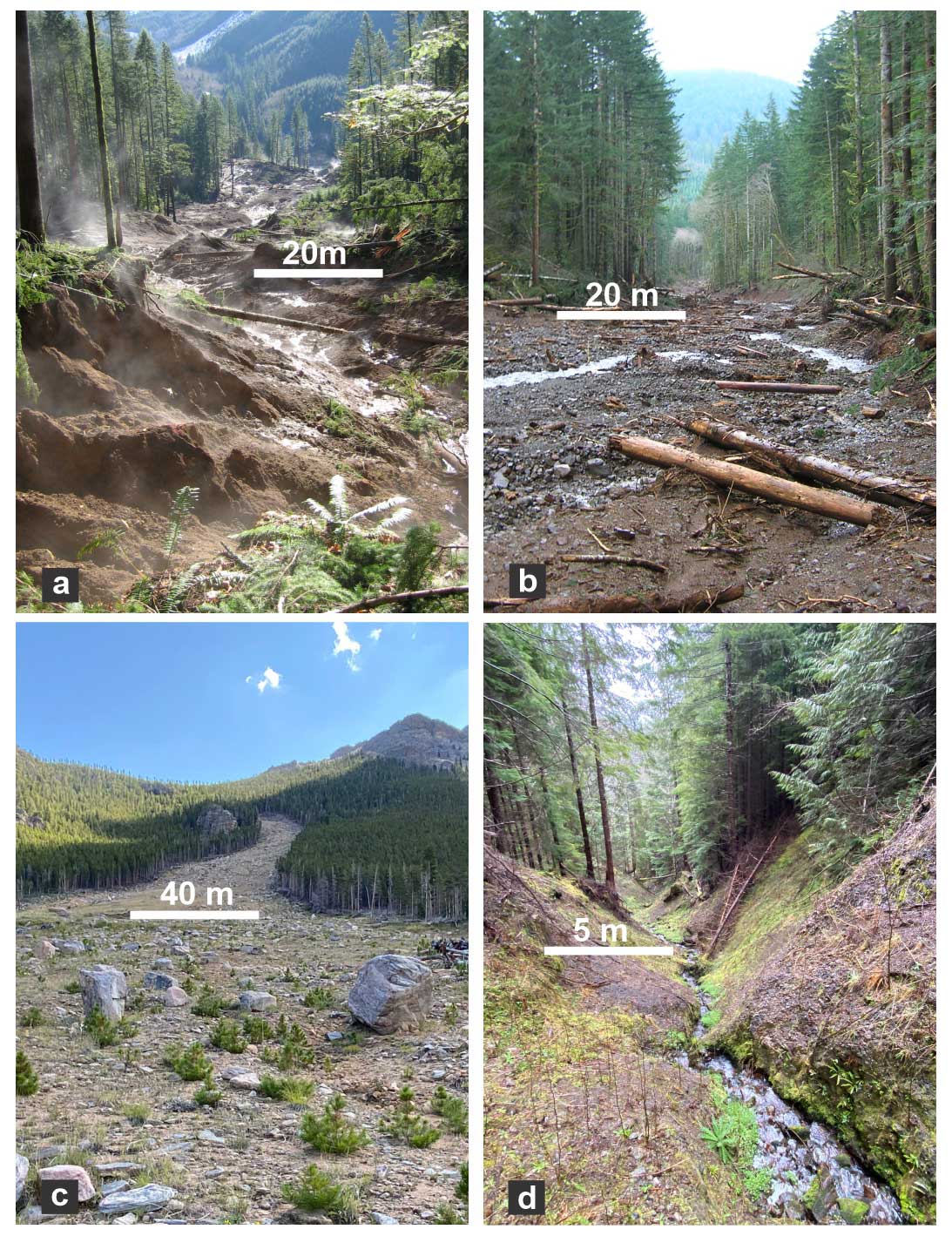
Figure 1 Example landslides used to evaluate calibrated MWR performance. (a) Cascade Mountains, WA: a large debris avalanche over steep, broadly convergent terrain (photo credit: Stephen Slaughter). (b) Black Hills, WA: large debris flows over a broadly convergent, gently sloped valley (photo credit: Stephen Slaughter). (c) Rocky Mountains, CO: a moderately sized debris avalanche over a steep, unconfined to divergent hillslope. (d) Olympic Mountains, WA: small debris flows in steep, highly convergent channels. Image scale varies with depth, but the approximate scale is indicated at the location of the scale bar.

2 Description of the MassWastingRunout model

2.1 Overview of the cellular-automaton modeling approach

MWR is coded as a discrete cellular-automaton (CA) model. CA models apply a set of equations or rules (deterministic or probabilistic) to individual cells of a grid to change the numerical or categorical value of a cell state (e.g., Codd, 1968). In earth sciences, CA models are widely used to model everything from vegetation dynamics (e.g., Nudurupati et al., 2023) and lava flows (e.g., Barca et al., 1993) to geomorphic transport, in which gravitationally directed erosion and depositional processes modify a digital elevation model (DEM) representation of a landscape (e.g., Chase, 1992; Crave and Davy, 2001; Murray and Paola, 1994; Tucker et al., 2018). Existing CA-based landslide runout models include models by Guthrie and Befus (2021), D'Ambrosio et al. (2003), and Han et al. (2021). In all of these models, runout behavior is controlled by topographic slope and rules for erosion and deposition, but conceptualization and implementation differ.

In MWR, mass continuity is central to model conceptualization. Of the wide range of landslide runout processes described in the Introduction, MWR explicitly represents erosion, deposition, and flow resistance as a function of the initial landslide body and downslope terrain. Material exchange between the runout material and underlying regolith as well as flow resistance determines runout extent and landscape evolution. Model rules are designed such that they can be parameterized from field measurements. Finally, in MWR, most computations occur only at the location of moving debris, in a manner analogous to the “mobile” cellular-automaton implementation of Chase (1992).

Chase (1992) modeled precipitation-driven surface erosion by randomly placing single packets of precipitation on a DEM, which then moved from higher-elevation to lower-elevation grid cells, eroding and transporting sediment as a function of the slope between the cells. The individual packets of precipitation were referred to as precipitons. In MWR, since we route the downslope progression of debris from a specified mass-wasting source area, we refer to these packets of debris as “debritons”. The debritons represent debris flux, here defined as a volume of debris transferred per model iteration per grid cell area, [m³ m⁻² per iteration], and are equivalent to the flow depth in the cell.

The present implementation of the MWR algorithm is coded in Python and developed as a component of the Landlab earth surface modeling toolkit (Barnhart et al., 2020; Hobley et al., 2017). MWR uses the Landlab raster model grid, which consists of a lattice of equally sized, rectangular cells. Topographic elevation, derived topographic properties like slope and curvature, and other spatially varying attributes such as regolith depth and grain size are recorded at nodes in the center of each cell (see Fig. 5 of Hobley et al., 2017). In the subsequent sections we describe the model theory. All parameters and variables used in the theory are listed in Table B1.

2.2 Mobilization of the initial mass-wasting source material (Algorithm 1)

To initiate MWR, the user provides maps of initial topography, regolith depth, and the location and depth of the mass-wasting source material (e.g., the initial landslide body). Each raster model grid node in the mass-wasting source material is designated as a debriton (Fig. 2, iteration t=0) with a magnitude equal to the mass-wasting source material depth at the node and basal elevation equal to the initial topography minus the mass-wasting source material depth at the node. The basal elevation can be thought to represent the rupture or slip surface of the source material, and the redistribution (flux) of each debriton to its downslope nodes (receiver nodes) is determined as a function of the slope of the slip surface. At the lowest-elevation debriton of the source material, flux to its downslope nodes is determined using the surface slope of the initial DEM (see the flow direction of the lowest node in Fig. 3a). This implementation helps to ensure that the lowest-elevation debriton in the mass-wasting source material moves downslope and movement of upslope debritons is impacted by the geometry of the mass-wasting source material. For example, the receiver nodes of the lowest-elevation debriton in the initial landslide body illustrated in Fig. 2 (node 45) would be identified as those among the eight neighboring nodes whose initial topographic elevation is less than the initial topographic elevation of node 45, while for the debriton at node 51, the receiver nodes would be identified as those among the eight neighboring nodes whose topographic elevation is less than the basal elevation of the debriton (see Fig. 3a).

Figure 2 Illustration of the mobilization and runout of an initial mass-wasting source area (landslide body) down a steep, convergent slope. Variable t indicates model iteration (not time). Notice how the flow elongates and widens as the model progresses and the number of receiver nodes (numbers listed at bottom of each panel) and quantity of mobilized material increase.

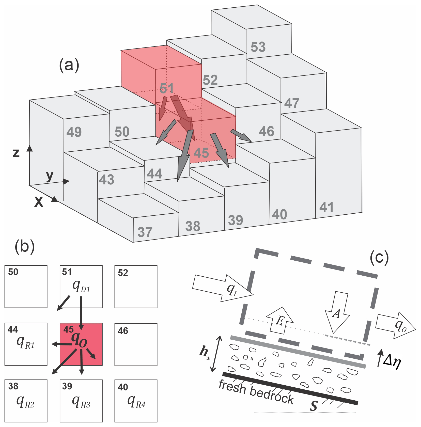
Figure 3 (a) Three-dimensional illustration of iteration t=0 in Fig. 2, showing initial source material nodes (represented by red cells) and flux towards downslope nodes. (b) Distribution of q₀ to downslope nodes 38, 39, 40, and 44; (c) illustration of mass continuity applied to any node that receives a debriton.

2.3 Flow routing and rules for erosion, deposition, and resistance (Algorithm 2)

Algorithm 2 is essentially the runout model. It determines how each debriton traverses and modifies the landscape. After receiver nodes from the first model iteration are determined in Algorithm 1 (iteration t=0), Algorithm 2 is repeatedly implemented until all material has deposited (i.e., there are no debritons). Each debriton moves one grid cell per model iteration; the larger the landslide size, the more iterations are necessary to evacuate the landslide slip surface. As each debriton moves, it may erode or aggrade the landscape, impacting the movement of any upslope debritons. As is common with other reduced-complexity models (e.g., Guthrie and Befus, 2021), we assume that inertial effects have a negligible impact on flow behavior (i.e., the kinematic flow approximation) and the downslope redistribution of a debriton or flux to each of a node's ith receiver nodes ($q_{R_i}$) is determined as a function of topographic slope (slope of the terrain under the debriton). We do this using the Freeman (1991) multiple-flow-direction algorithm:

$$\begin{array}{}\text{(1)}& q_{R_i}=q_{\mathrm{O}}{\displaystyle \frac{S_i^a}{{\sum }_{i=\mathrm{1}}^{\text{Nr}}{S}_i^a}},\end{array}$$

where q_O is the total outgoing flux from the node and has units of depth in meters per model iteration, Nr is the number of receiving nodes, i is the index for each receiver node (e.g., $i=\mathrm{1},\mathrm{2}\mathrm{\dots }\text{Nr}$), and S_i is the underlying topographic slope to the ith receiver node (Fig. 3b). The Freeman (1991) multiple-flow-direction algorithm is a commonly used approximation for two-dimensional flow, and in this implementation it is handled by a pre-existing Landlab flow-routing component. The exponent a controls how material is distributed to downslope nodes, with higher values causing narrower flow (Holmgren 1994). In a braided river cellular-automaton model, Murray and Paola (1997) used an approximation for turbulent shallow-water flow to justify a=0.5 (which is the exponent on the slope factor in channel friction laws). For our application, we found that MWR provided a closer fit to observed mass-wasting runout if a=1, suggesting that the material behavior is more similar to linear–viscous shear flow than to wall-bounded turbulent shear flow (e.g., as the runout debris flows downslope, it tends to spread less than shallow, turbulent water). The total incoming flux (again, in units of meters per model iteration) towards a given node (q_I) is determined by summing the flux from each of the node's donor nodes:

$$\begin{array}{}\text{(2)}& q_I={\sum }_{j=\mathrm{1}}^{\text{Nd}}{q}_{D_j},\end{array}$$

where Nd is the number of donor nodes, and $q_{D_j}$ is the flux from node D_j (the jth donor node, $j=\mathrm{1},\mathrm{2}\mathrm{\dots }\text{Nd}$; Fig. 3b).

As noted by Tucker and Hancock (2010), the flow depths calculated from two-dimensional flow approximations as in Eq. (1) can be influenced by the choice of grid size used to represent the terrain. Additionally, as simplified multi-directional flow models as in Eq. (1) neglect the pressure and momentum forces in the movement of flow, they can result in inaccurate flow width and depth estimates, depending on terrain slope and convergence. Rengers et al. (2016) noted these limitations when using a kinematic wave approximation of the shallow-water equations, as this approximation lacks a pressure term that facilitates the spreading of the modeled water surface. While the topographic controls on mass conservation are adequately represented by Eq. (1), our model bears such limitations when calculating flow depth and width. Moreover, in our model, flow depth is used to determine a depth-dependent erosion rate. As such, in order to avoid unrealistically high flow depths (and erosion rates), we constrain flow depth to an upper limit as

$$\begin{array}{}\text{(3)}& h=min(h_{\text{max}},q_I),\end{array}$$

where h_max is an effective upper limit to flow depth that in practice can be approximated as the maximum observed flow depth, as inferred from field indicators or assigned based on expert judgment (see Sect. 5), and h is the corrected flow depth used to calculate flow shear stress. This correction allows erosion rates to vary with flux but prevents unreasonably large values. This flow depth correction does not violate the conservation of mass and runout mass balance, as h is only used to calculate flow shear stress.

To determine aggradation (A) at a node, we use a critical slope (S_c) constraint that permits computationally rapid distribution of q_I over multiple nodes. Critical slope constraints or rules are common to many reduced-complexity and landscape evolution models. Chen et al. (2023) showed that when flow inertia can be ignored, S_c can be approximated from the surface slope of observed deposits. Several landscape evolution models use an S_c-based nonlinear, nonlocal aggradation scheme (e.g., Campforts et al., 2020; Carretier et al., 2016), but when this rule is implemented with the debriton framework described above, unreasonably tall deposits result when q_I is large and the slope at the node (S)≪S_c. To resolve this problem, aggradation depth can be limited to A≤S_cΔx (where Δx is the grid cell length), but we found that this constraint results in long deposits that parallel the underlying slope when q_I is large. Instead, MWR computes the aggradation depth at a node assuming that the aggradation will spread over N_a nodes until all of q_I is deposited and that the surface slope of the overall deposit will be equal to S_c, as shown in Fig. 4 and described as follows.

Figure 4 Illustration of the aggradation rule used in MWR when q_I is assumed to spread over five nodes (N_a=5). The solid yellow box indicates aggradation amount at a given node. Dashed yellow boxes and lines indicate the geometry of assumed aggradation beyond the node. Dots along the DEM surface are nodes.

Aggradation at a node is determined as

$$\begin{array}{}\text{(4)}& A=\left\{\begin{array}{ll}\mathrm{0},& S\ge S_{\mathrm{c}}\\ min\left(A_{\mathrm{p},N_{\mathrm{a}}},q_I\right),& S<S_{\mathrm{c}},\end{array}\right.\end{array}$$

where S is the steepest slope to the node's eight neighboring nodes, and $A_{\mathrm{p},N_{\mathrm{a}}}$ is a potential aggradation depth necessary to form the beginning of the overall deposit that (1) begins at the node and spreads over N_a consecutive nodes, (2) has a total volume equal to q_IΔx², (3) has a surface slope equal to the critical slope S_c, and (4) has an underlying topographic slope equal to S that is assumed to be constant over the N_a consecutive nodes of deposition. From these assumptions, we can analytically define $A_{\mathrm{p},N_{\mathrm{a}}}$ and N_a as a function of q_I, S_c, and S as follows.

First, q_I, calculated from Eq. (2), can be used to calculate A_p,i by expressing q_I as the sum of the N_a deposits that make up the overall deposit as

$$\begin{array}{}\text{(5)}& q_I={\sum }_{i=\mathrm{1}}^{N_{\mathrm{a}}}{A}_{\mathrm{p},i},\end{array}$$

where A_p,i is the ith deposition amount in the overall deposit and i=1 is the last node of deposition (A_p,1; see Fig. 4). Since we assume the deposit slope and underlying topographic slope are uniform, the deposition amount at any of the N_a nodes can be determined from A_p,1 as

$$\begin{array}{}\text{(6)}& A_{\mathrm{p},i}=A_{\mathrm{p},\mathrm{1}}+(i-\mathrm{1})\mathrm{\Delta }x(S_{\mathrm{c}}-S).\end{array}$$

From Eq. (6) we can rewrite Eq. (5) as a function of A_p,1 and rearrange to define A_p,1 as a function of q_I:

$$\begin{array}{}\text{(7)}& A_{\mathrm{p},\mathrm{1}}={\displaystyle \frac{\mathrm{1}}{N_{\mathrm{a}}}}{q}_I-{\displaystyle \frac{N_{\mathrm{a}}-\mathrm{1}}{\mathrm{2}}}\mathrm{\Delta }x(S_{\mathrm{c}}-S).\end{array}$$

Substituting Eq. (7) into Eq. (6) and solving for i=N_a, we get an expression for $A_{\mathrm{p},N_{\mathrm{a}}}$:

$$\begin{array}{}\text{(8)}& A_{\mathrm{p},N_{\mathrm{a}}}={\displaystyle \frac{\mathrm{1}}{N_{\mathrm{a}}}}{q}_I+{\displaystyle \frac{N_{\mathrm{a}}-\mathrm{1}}{\mathrm{2}}}\mathrm{\Delta }x\left(S_{\mathrm{c}}-S\right).\end{array}$$

Equation (8) can be rearranged into a quadratic equation and solved for N_a as

$$\begin{array}{}\text{(9)}& N_{\mathrm{a}}={\displaystyle \frac{-A_{p,\mathrm{1}}+\frac{\mathrm{1}}{\mathrm{2}}\mathrm{\Delta }x\left(S_{\mathrm{c}}-S\right)\pm \sqrt{{\left(A_{\mathrm{p},\mathrm{1}}-\frac{\mathrm{1}}{\mathrm{2}}\mathrm{\Delta }x\left(S_{\mathrm{c}}-S\right)\right)}^{\mathrm{2}}+\mathrm{2}\mathrm{\Delta }x\left(S_{\mathrm{c}}-S\right)q_I}}{\mathrm{\Delta }x\left(S_{\mathrm{c}}-S\right)}}.\end{array}$$

We use Eq. (8) to solve for $A_{\mathrm{p},N_{\mathrm{a}}}$ and Eq. (9) to solve for N_a assuming $A_{\mathrm{p},\mathrm{1}}=\mathrm{1}/\mathrm{2}\mathrm{\Delta }x{S}_{\mathrm{c}}$ and rounding the positive solution to the nearest integer. When implemented using a single debriton released on a two-dimensional hillslope as illustrated in Fig. 4, the debriton deposits over N_a nodes at a uniform slope equal to S_c. When implemented on an actual three-dimensional terrain, the interaction between multiple debritons in multiple directions creates a complex deposit whose slope changes with S_c.

To determine erosion depth (E) [m per iteration], we constrain E to the lesser of a potential erosion depth, h_e, and local regolith depth, h_r:

$$\begin{array}{}\text{(10)}& E=min\left(h_{\mathrm{r}},h_{\mathrm{e}}\right),\end{array}$$

where h_e is computed as a function of the basal shear stress of the flow, τ [Pa] (Eqs. 12 and 13), and the critical shear stress (τ_c) of the regolith at the node [Pa],

$$\begin{array}{}\text{(11)}& h_{\mathrm{e}}=k(\mathit{\tau }-{\mathit{\tau }}_{\mathrm{c}}{)}^f.\end{array}$$

The coefficient k is an erodibility parameter [m Pa^−f]. Stock and Dietrich (2006) showed that k encapsulates substrate properties. If h_e is used to represent erosion over geomorphic timescales, with repeated debris flow occurrences in a single model iteration, k becomes associated with debris flow length and frequency (Perron, 2017). In our application since we are modeling the erosion associated with a single runout event, as represented by the downslope movement of the debritons, the coefficient k therefore needs to scale h_e on the order of the average erosion depth caused by a single debriton. Using this logic, k can be computed using the observed average erosion depth and an estimated length of the runout material that caused the erosion. Further details on how we determine k from observed runout are included in Appendix A. The exponent f controls the nonlinearity of h_e with shear stress. Many authors (e.g., Chen and Zhang, 2015; Frank et al., 2015; Shen et al., 2020) use a value of 1 for f but field measurements by Schürch et al. (2011) (see their Fig. 3) suggest that f may be less than 1 if τ is assumed to vary linearly with flow depth, particularly at flow depths greater than 3 m.

MWR includes two options for defining τ: (1) a quasi-static basal shear stress approximation or (2) a grain-size-based shear stress approximation. The quasi-static basal shear stress approximation (e.g., Takahashi, 2014) is defined as

$$\begin{array}{}\text{(12)}& \mathit{\tau }=\mathit{\rho }gh\sin \mathit{\theta },\end{array}$$

where ρ is the density of mass-wasting material (grain and water mixture) [kg m⁻³], g is gravity [m s⁻²], h is the adjusted flow depth described in Eq. (3), and θ is the topographic slope (tan ⁻¹(S)) measured in degrees.

The grain-size-based shear stress approximation is defined using an empirical formula by Bagnold (1954):

$$\begin{array}{}\text{(13)}& \mathit{\tau }=\mathit{\sigma }\tan \mathit{\phi },\end{array}$$

where σ is normal stress [Pa], and φ is the collision angle between grains measured from the vertical axis (see Bagnold, 1954) with a value of tan φ typically equal to 0.32. Stock and Dietrich (2006) defined σ as

$$\begin{array}{}\text{(14)}& \mathit{\sigma }=\cos \mathit{\theta }{\mathit{\upsilon }}_{\mathrm{s}}{\mathit{\rho }}_{\mathrm{s}}{D}_{\mathrm{s}}^{\mathrm{2}}{\left({\displaystyle \frac{\mathrm{d}u}{\mathrm{d}z}}\right)}^{\mathrm{2}},\end{array}$$

where υ_s is the volumetric solid concentration, ρ_s is density of the solids [kg m⁻³], u is flow velocity [m s⁻¹], z is depth below the flow surface [m], $\mathrm{d}u/\mathrm{d}z$ is the shear strain rate [s⁻¹], and D_s is the representative grain size [m]. Stock and Dietrich (2006) suggested that D_s corresponds to a small percentile of the coarsest fraction of the runout material (D₈₈ to D₉₆) and they approximated $\mathrm{d}u/\mathrm{d}z$ as

$$\begin{array}{}\text{(15)}& {\displaystyle \frac{\mathrm{d}u}{\mathrm{d}z}}={\displaystyle \frac{u}{h}}.\end{array}$$

Solely for the purpose of computing $\mathrm{d}u/\mathrm{d}z$, we approximate velocity at a node using a grain-size-dependent empirical formula for debris flow velocity by Julien and Paris (2010) as

$$\begin{array}{}\text{(16)}& u=\mathrm{5.75}{u}^{\ast }\log \left({\displaystyle \frac{h}{D_{\mathrm{s}}}}\right),\end{array}$$

where u^∗ is shear velocity $\left(\sqrt{gh\tan \mathit{\theta }}\right)$. Substituting Eqs. (16), (15), (14), and (13) into Eq. (11) yields a grain-size-dependent approximation for h_e that mimics the nonlinear erosion response to flow depth in Schürch et al. (2011). Additionally, this form of τ is advantageous because it permits landslide-driven erosion rates to scale with landslide grain size, which can vary by lithologic region (e.g., Roda-Boluda et al., 2018). As will be shown in Sect. 5, we obtained reasonable model calibration at multiple sites by defining D_s from the coarser grain sizes observed in the field at existing runout deposits, road cuts, and tree-throw pits.

Once A [m] and E [m] have been determined, total outgoing flux per iteration, q_O [m], is determined as (see Fig. 3c)

$$\begin{array}{}\text{(17)}& q_{\mathrm{O}}=\left\{\begin{array}{ll}{q}_I-A+E,& q_I\ge q_{\mathrm{c}}\\ \mathrm{0}& q_I<q_{\mathrm{c}},\end{array}\right.\end{array}$$

where q_c is a threshold flux for deposition. When q_I<q_c, q_I deposits and q_O becomes zero. The threshold flux q_c conceptually represents the flow depth below which flow resistance is large enough to cease the forward momentum of the flow, whether in the form of internal friction or friction due to vegetation and obstructions (e.g., large clasts or logs). The density and water content of q_I, A, and E are treated as uniform, and surface runoff, such as channelized stream flow or hillslope infiltration excess runoff, that might mix with q_I, A, or E is ignored. Once q_I, A, q_O, and E have been determined, change in elevation at a node (Δη) is calculated as

$$\begin{array}{}\text{(18)}& \mathrm{\Delta }\mathit{\eta }=A-E.\end{array}$$

Attributes (e.g., grain size, organic content, or any other attribute that is transferred in the flow) of the debriton and regolith are updated using a volumetric-weighted average approach. First, for each regolith attribute being tracked by the model, the attribute value delivered to a node from its donor nodes (ξ_D) is determined as

$$\begin{array}{}\text{(19)}& {\mathit{\xi }}_D={\displaystyle \frac{{\mathit{\xi }}_D*{\mathit{q}}_D}{q_I}},\end{array}$$

where q_D is a vector containing each $q_{D_j}$ sent to the node, ξ_D is a vector containing the incoming attribute values for each $q_{D_j}$, and q_I is the sum of incoming flux from donor nodes defined by Eq. (2).

Second, the attribute value sent from a node to its receiver nodes (ξ_R) is determined as

$$\begin{array}{}\text{(20)}& {\mathit{\xi }}_R={\displaystyle \frac{{\mathit{\xi }}_{t-\mathrm{1}}E+{\mathit{\xi }}_D(q_I-A)}{q_{\mathrm{O}}}},\end{array}$$

where ξ_t−1 is the attribute value at the node before any aggradation (i.e., the previous iteration attribute value). Finally, the attribute value at the node, updated to account for erosion and aggradation (ξ), is

$$\begin{array}{}\text{(21)}& \mathit{\xi }={\displaystyle \frac{{\mathit{\xi }}_{t-\mathrm{1}}\left(h_{\mathrm{r}}-E\right)+{\mathit{\xi }}_{D}A}{A+h_{\mathrm{r}}-E}}.\end{array}$$

Regolith thickness (h_r) and topographic elevation (η) are updated at a node as

$$\begin{array}{}\text{(22)}& \mathit{\eta }={\mathit{\eta }}_{t-\mathrm{1}}+\mathrm{\Delta }\mathit{\eta },\end{array}$$

$$\begin{array}{}\text{(23)}& h_{\mathrm{r}}=h_{rt-\mathrm{1}}+\mathrm{\Delta }\mathit{\eta },\end{array}$$

where η_t−1 and h_rt−1 are the topographic surface elevation and regolith thickness at the node from the previous model iteration. After regolith thickness and topographic elevation have been updated for each debriton, the multi-direction slope of the DEM, which is needed for implementing Eq. (1) in the next model iteration, is recomputed.

As the DEM is updated following each model iteration, topographic pits or flat topography may form. These features have no slope or slope inwards and obstruct debriton movement. To allow a debriton to pass an obstruction, we rely on a simple workaround: upon encountering the obstruction, the debriton is directed to itself and some portion of the debris is deposited based on Eq. (4). At the end of the model iteration, the node elevation and slope are updated. During the next iteration, if the remaining mobile debris is no longer obstructed, it moves to its downslope node(s). If the node is still obstructed, it is again sent to itself until either all material has deposited or the elevation of the node exceeds that of its neighbor nodes, allowing the debriton to move downslope.

3 Calibration and MWR Probability

3.1 Calibration utility

MWR includes a calibration utility that uses an adaptive Bayesian Markov chain Monte Carlo (MCMC) algorithm described by Coz et al. (2014) and Renard et al. (2006). The calibration utility determines (1) a single set of parameters that best match MWR output to an observed landslide runout dataset and (2) posterior parameter probability distribution functions (PDFs). The observed runout dataset can consist of a single landslide or multiple landslides. Depending on user input, MWR simultaneously or sequentially models runout from each landslide source area in one model run. To use the calibration utility, the user provides an initial (prior) guess of the parameter values and their respective PDFs that calibrate the MWR to a specific site. Then, the calibration utility randomly selects a set of trial parameter values (Λ) from the prior PDFs and runs MWR using Λ. Once the model has completed the run, the algorithm evaluates the posterior likelihood of the parameter set (L(Λ)) as the product of model ability to replicate observed runout (described below) and the prior likelihood of the parameter set. After the first L(Λ) has been determined, the utility selects a new set of parameters (Λ_t+1) by jumping some distance (described below) from each parameter in Λ space. Depending on the value of L(Λ_t+1), the algorithm either stays at Λ or moves to Λ_t+1. This Markov process is repeated a user-specified number of times. The jump direction is random, but the algorithm is adaptive because the jump distance changes depending on whether $L\left({\mathrm{\Lambda }}_{t+\mathrm{1}}\right)>L\left(\mathrm{\Lambda }\right)$ occurs more than a user-specified threshold value. For a detailed description of the algorithm see Coz et al. (2014).

The L(Λ) index is estimated as the product of the prior probability of the selected parameter values, p(Λ), and three other performance metrics as

$$\begin{array}{}\text{(24)}& L\left(\mathrm{\Lambda }\right)=p\left(\mathrm{\Lambda }\right)\cdot {\mathrm{\Omega }}_T\cdot {\displaystyle \frac{\mathrm{1}}{\mathrm{\Delta }{\mathit{\eta }}_{\mathrm{E}}^{\mathrm{2}}}}\cdot {\displaystyle \frac{\mathrm{1}}{Q_{{\mathrm{s}}_{\mathrm{E}}}^{\mathrm{2}}}},\end{array}$$

where Ω_T is an index for evaluating model planimetric fit described by Heiser et al. (2017), and Δη_E and $Q_{{\mathrm{s}}_{\mathrm{E}}}$ are new dimensionless indices proposed for this study (described below). The index Δη_E is the volumetric error of the modeled topographic change over the entire model domain normalized by the observed total mobilized volume (initial landslide body + erosion volume). The index $Q_{{\mathrm{s}}_{\mathrm{E}}}$ is the mean cumulative sediment transport error along the modeled runout path normalized by the observed mean cumulative flow. Larger values of Ω_T and smaller values of Δη_E and $Q_{{\mathrm{s}}_{\mathrm{E}}}$ indicate that modeled runout more closely fits observed. Note that we add a value of 1 to Ω_T and use the squared reciprocal values of Δη_E and $Q_{{\mathrm{s}}_{\mathrm{E}}}$ in Eq. (24) so that the magnitude of L(Λ) is always equal to or greater than zero and increases with improved fit. The metric Ω_T is written as

$$\begin{array}{}\text{(25)}& {\mathrm{\Omega }}_T={\displaystyle \frac{\mathit{\alpha }-\mathit{\beta }-\mathit{\gamma }}{\mathit{\alpha }+\mathit{\beta }+\mathit{\gamma }}}+\mathrm{1},\end{array}$$

where α, β, and γ are the areas of matching, overestimated, and underestimated runout extent, respectively.

The index Δη_E is determined as

$$\begin{array}{}\text{(26)}& \mathrm{\Delta }{\mathit{\eta }}_{\mathrm{E}}=\sqrt{{\displaystyle \frac{{\sum }_{i=\mathrm{0}}^p\left[\right(\mathrm{\Delta }{\mathit{\eta }}_{\mathrm{O}i}-\mathrm{\Delta }{\mathit{\eta }}_{\mathrm{M}i})\mathrm{\Delta }{x}^{\mathrm{2}}{]}^{\mathrm{2}}}{V^{\mathrm{2}}}}},\end{array}$$

where V is observed total mobilized volume and p is the number of nodes in the area made up of the matching, overestimated, and underestimated areas of modeled runout extent. Δη_Mi and Δη_Oi are the modeled and observed topographic change [m] at the ith node within that extent.

To calculate $Q_{{\mathrm{s}}_{\mathrm{E}}}$, we first determine the cumulative sediment transport volume (Q_s) at each node, j along the runout profile, in a manner similar to the flow volume–mass balance curves in Fannin and Wise (2001) and Hungr and Evans (2004):

$$\begin{array}{}\text{(27)}& Q_{\mathrm{s}}=-\mathrm{\Delta }{x}^{\mathrm{2}}{\sum }_{i=\mathrm{1}}^{u_j}\mathrm{\Delta }{\mathit{\eta }}_{i,j},\end{array}$$

where Δη_i,j is the topographic change [m] at the ith node located above the elevation of node j, and u_j is the total number of nodes located above node j. Q_s is computed for both the observed and modeled runout (Q_sO and Q_sM, respectively) and $Q_{{\mathrm{s}}_{\mathrm{E}}}$ is determined as

$$\begin{array}{}\text{(28)}& Q_{{\mathrm{s}}_{\mathrm{E}}}=\sqrt{{\displaystyle \frac{\frac{\mathrm{1}}{r}{\sum }_{j=\mathrm{1}}^r{\left(Q_{\text{sO}}-Q_{\text{sM}}\right)}^{\mathrm{2}}}{{\stackrel{\mathrm{‾}}{Q_{\text{sO}}}}^{\mathrm{2}}}}},\end{array}$$

where r is the number of nodes along the runout profile, and $\stackrel{\mathrm{‾}}{Q_{\text{sO}}}$ is the observed mean cumulative flow.

As will be detailed in Sect. 5, field estimates for S_c and q_c vary over the length of the runout path. To account for the heterogeneity of S_c and q_c, we estimate prior PDFs of potential S_c and q_c values from field and/or remote sensing measurements. Then, from model calibration to a DEM of difference (pre-runout DEM subtracted from the post-runout DEM; DoD) using the calibration utility, we produce posterior PDFs of S_c and q_c and find a single S_c and q_c pair that allows the modeled DoD to best replicate the observed DoD (i.e., the S_c and q_c pair with the highest L(Λ) value).

We run the calibration utility using a single Markov chain of 2000 repetitions. At most sites, the model converged relatively quickly on a solution and we therefore did not account for burn-in or evaluate convergence (e.g., Gelman et al., 2021) and considered 2000 repetitions adequate. Future implementations of the calibration utility may include multiple chains, burn-in, and a check for convergence. As a final note, many debris flow runout models are evaluated using Ω_T or variations of Ω_T alone (e.g., Gorr et al., 2022; Han et al., 2017) and the MWR calibration utility can also be run solely as a function of Ω_T (i.e., runout extent). However, we found that calibration based on Ω_T alone results in high parameter equifinality (e.g., Beven 2006); multiple parameter sets result in an equally calibrated model as evaluated by Ω_T. As such, we recommend calibrating debris flow and landslide runout models to an observed DoD. If repeated lidar is available, a DoD can be obtained from before and after scans of the observed runout event. Alternatively, a DoD can be created by hiking the observed runout event and mapping field-interpreted erosion and deposition depths. Additional details on how we prepared DoDs for multiple sites are included in the Supplement.

3.2 Mapping landslide runout hazard

MWR includes an additional utility called MWR Probability that produces landslide runout probability maps. MWR Probability repeatedly runs MWR a user-specified number of times (Np), each repetition with a different, randomly sampled parameter set from the posterior parameter PDFs produced by the calibration utility. MWR Probability includes three options for specifying the initial mass-wasting source material: (1) a user-provided landslide source area polygon based on field and/or remote sensing observations; (2) a user-defined hillslope that is susceptible to landslides (e.g., potentially unstable slope), where landslide area and location are randomly selected within but no larger than the hillslope – this option is useful when the extent of a potential landslide is unknown; and (3) a series of mapped landslide source areas within a watershed, as determined by an externally run Monte Carlo landslide initiation model (e.g., Hammond et al., 1992; Strauch et al., 2018) – this option is useful for regional runout hazard applications. If using Option 1, modeled runout probability represents uncertainty in MWR parameterization. If using Option 2 or 3, modeled runout probability reflects uncertainty in both MWR parameterization and landslide location and size.

For all three run options, each model iteration begins with the same initial topography. After Np model simulations, Np different versions of the post-runout landscape are created, and the probability of runout at each node is determined as

$$\begin{array}{}\text{(29)}& P\left(\mathrm{\Delta }\mathit{\eta }\right)={\displaystyle \frac{\text{num}\left(\left|\mathrm{\Delta }\mathit{\eta }\right|>\mathrm{0}\right)}{\mathrm{Np}}},\end{array}$$

where num(|Δη|>0) is the number of times topographic elevation at a node changes as a result of erosion or deposition from the Np model runs. Probability of erosion or aggradation can be determined by replacing the numerator in Eq. (29) with num(Δη<0) or num(Δη>0), respectively.

4 Basic model behavior

We evaluate basic model behavior using a series of virtual experiments. The virtual experiments consist of six synthetic terrains, including (a) a planar slope that intersects a gently sloped plane (S=0.001), (b) a planar slope with a constriction that intersects a gently sloped plane, (c) a planar slope that has a bench mid-slope and then intersects a gently sloped plane, (d) a concave-up uniform-convergence slope, (e) a concave-up variable-convergence slope that widens (convergence decreases) in the downslope direction, and (f) a convex-up variable-convergence slope that widens (convergence decreases) in the downslope direction. On each terrain, a 30 m wide, 50 m long, and 3 m deep landslide is released from the top of the terrain. All six terrains are covered by a 1 m thick regolith and use the same parameter values (S_c=0.03, q_c=0.2 m, k=0.01, D_s=0.2 m). Each terrain is represented using a 10 m grid. Experiment results are shown in Fig. 5.

Figure 5 Shaded, 3-D visualizations of model response to six different synthetic terrains, colored according to the DoD of the final runout surface. Shading is to scale. Red indicates a positive change in the elevation of the terrain (aggradation) and blue indicates a negative change (erosion). The 3-D visualization of the DoD is exaggerated by a factor of 5 to make it visible in the figure. Grid size is 10 m.

On Terrain A, the landslide spread as it moved downslope and formed levees along the edge of the runout path. The width of the spread was a function of the multiple-flow-direction algorithm and resistance along lateral margins of the runout as represented by q_c. At the slope break at the base of the slope, the material deposited at an angle controlled by S_c. On Terrain B, the flow initially eroded and deposited material identical to Terrain A, but near the slope break, the topographic constriction forced flow depth to increase and exceed q_c, minimizing the formation of levees (because q_O>q_c), and resulted in a slightly larger deposit at the base of the slope. On Terrain C, landslide runout was again initially identical to the runout on Terrain A; however, upon intersecting the mid-slope bench, most of the runout material deposited. A small, thinner portion did continue past the bench but eroded at a lower rate than upslope of the bench. Upon intersecting the flat surface at the base of the hillslope, the runout material was deposited.

On Terrain D, the landslide and its runout were confined to the center of the convergent terrain and were only deposited once the slope was less than S_c. The slide never widened because the uniformly convergent channel shape prevented spreading and the narrower flow width maintained a higher flow depth, which prevented the formation of levees. On Terrain E, the landslide again deposited once the slope was less than S_c, but because topographic convergence of Terrain E decreases in the downslope direction, as the runout material moved downslope, the deposit spread more than on Terrain D, which caused thinner flow and deposition along margins of the runout path. On the final terrain, Terrain F, the slope is always greater than S_c, so deposition was limited to levees along the edge of the flow that formed as the runout spread in response to decreasing convergence.

MWR model behavior can be summarized as follows: the displacement and deposition of landslide material predicted by MWR respond to topography in a reasonable manner. Flow width increases as convergence decreases (e.g., Terrain F), which in turn reduces flow depth. Lower flow depths cause lower erosion rates and reduce aggradation extent. Conversely, modeled flow depth increases when convergence increases (e.g., Terrain B). Where the flow encounters broadly convergent or planar slopes, lateral levee deposits form, a common feature of landslides reported in the literature and at sites reported here (see Sect. 5) that detailed mechanistic models can struggle to reproduce (e.g., Barnhart et al., 2021).

We do not attempt to compare MWR modeled flow with the output of shallow-water-equation-based models or observed granular flows (e.g., Medina et al., 2008; McDougall and Hungr, 2004; Iverson and Denlinger, 2001; Han et al., 2015). The cellular-automaton representation in MWR does not model the time-dependent evolution of debris flow velocity and depth, and it conceptually moves debris instantaneously at each iteration, as driven by changes in the evolving topographic elevation field. Because of that, only the final outcome (modeled runout extent, sediment transport, and topographic change) of MWR can be compared with other models or observed runout, which we do in the next section. Also, as described in Sect. 2.3, the behavior of the multiple flow direction algorithm does vary with grid size. Using a coarser or finer grid, without adjusting model parameterization, could potentially change the runout patterns shown in Fig. 5.

5 Model validation

5.1 Overview

In this section, we demonstrate the ability of a calibrated MWR to replicate observed runout extent, sediment transport, and topographic change at field sites located in the western USA and summarize model calibration results with an evaluation of MWR calibration relative to terrain attributes of the observed runout paths. Note that simply calibrating a model to match field data does not constitute a satisfactory test of model predictive ability (Iverson, 2003). Strategic testing, which involves calibrating the model to one site or period of time and then running the calibrated model at a separate site or period of time (Murray, 2013), is a better indicator. Two of our validation sites, the Cascade Mountains and Olympic Mountains sites, include two separate landslides and subsequent runout and we test model predictive ability at these sites in Sect. 6.

Calibrated model performance is demonstrated at the following field sites (see Fig. 6a for locations and observed runout extent): (1) two runout events over the same hillslope in the Cascade Mountains (Washington state – WA, USA) – a large debris avalanche in 2009 (Cascade Mountains, 2009) and a moderately sized debris flow in 2022 (Cascade Mountains, 2022) that inundated and flowed within a first- to second-order channel until perpendicularly intersecting a narrow river valley several hundred meters below the landslide (Fig. 1a); (2) debris flows in the Black Hills (WA) sourced from a small failure along the toe of a deep-seated landslide (Black Hills, south) and a moderately sized debris avalanche from a large road fill (Black Hills, north) that flowed several kilometers along a relatively wide, broadly convergent channel before stopping (Fig. 1b); (3) a single, moderately sized debris avalanche in the Rocky Mountains (Rocky Mountains), the majority of which flowed several hundred meters over a broadly convergent to divergent hillslope in Colorado (Fig. 1c); and (4) a 30-year chronology of small landslides and subsequent debris flows in the Olympic Mountains (WA) in steep, highly convergent channels that flowed well over a kilometer and coalesced into a single runout deposit in a dendritic, channelized watershed (Olympic Mountains; Fig. 1d). All landslides were initiated during heavy rainfall or rain-plus-snowmelt storm events (WRCC, 2024; NRCS, 2022; Table 1), but their runout varied in terms of erosion rate, grain size (Fig. 6b), depositional behavior (Fig. 6c), and the topographic convergence of the underlying terrain.

Table 1 Landslide and runout characteristics.

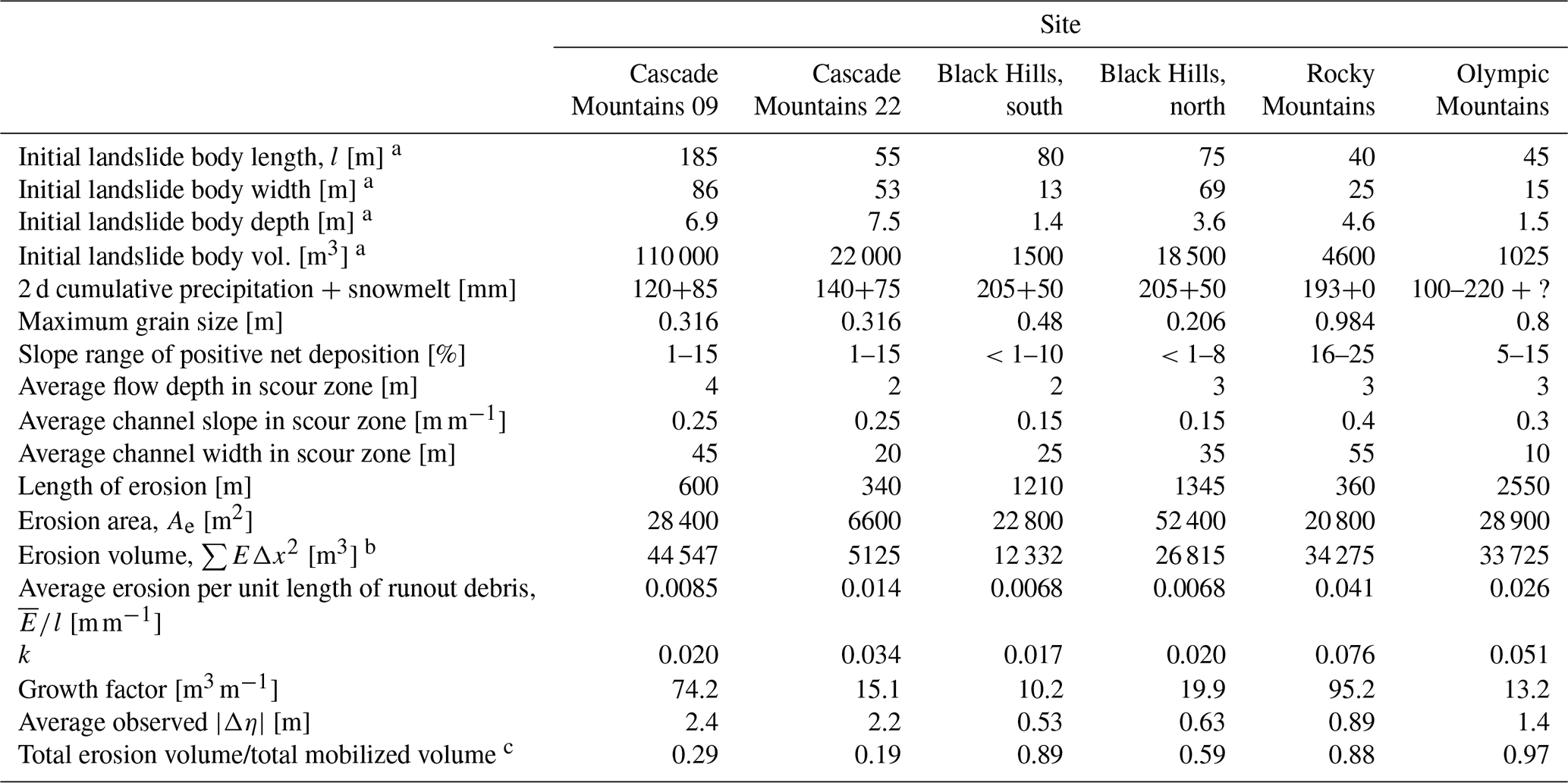
^a For the Olympic Mountains site, width and depth are average values and length and volume are defined as the average cumulative value upstream of each runout path. ^b Excludes landslide volume. ^c Total mobilized volume=initial landslide body + erosion volume.

Figure 6 (a) Landslide locations in Washington and Colorado. Coordinates next to each site are WGS84. Shaded DEMs of each site are shown at the same scale. (b) Observed average erosion rate per unit landslide length ($\stackrel{\mathrm{‾}}{E}/l$) relative to the observed average maximum grain size. Error bars indicate standard deviation. (c) Underlying topographic slope of observed deposition.

5.2 Model setup and field parameterization

Each model was set up on a 10 m grid representation of the pre-event DEM with either a uniform or spatially varying regolith thickness (detailed for each site in the Supplement). The length (l) and area of the initial mass-wasting source material (e.g., the initial landslide body) were interpreted from a combination of lidar DEM, air photos, and field observations. The average depth of the initial landslide body was measured in the field or from the DoD. The volume of the initial landslide body was determined as the area times the average depth. An average width was determined as the area divided by the length. At the Olympic Mountains site, where the observed runout pattern formed as a result of multiple landslides (see the Supplement), landslide depth and width values listed in Table 1 are average values, and landslide length, area, and volume values are the average cumulative value upstream of each runout path. At all locations, we use Eq. (13) to approximate shear stress. We field-surveyed each site, noting the maximum flow depth (inferred from initial landslide body volume and height of scour marks as well as width of the channel in the erosion zone), typical deposition and erosion depths, and the size of the largest grains in the runout deposits.

We estimated parameter values from these field and remote observations (see Table 1). A site-specific value for k was determined as a function of the observed average erosion depth (determined as total erosion volume divided by the erosion area, $\stackrel{\mathrm{‾}}{E}$) relative to the length of the runout debris, which we approximated as the length of the initial landslide body (l). Further details are described in the Appendix.

The volume of the initial landslide body ranged from 400 to 110 000 m³ across sites. At all sites, erosion and subsequent entrainment added to the total mobilized volume (initial landslide body + erosion volume), but the contribution was highly variable. The erosion volume divided by the total mobilized volume was as low as 0.19 for the Cascade Mountains 2022 landslide and as high as 0.97 for the Olympic Mountains landslides (Table 1).

The average maximum grain size varied from 0.2 m at the Black Hills sites to nearly 1 m at the Rocky Mountains site (Fig. 6b, Table 1). Values of $\stackrel{\mathrm{‾}}{E}/l$ ranged from 0.007 to 0.041 [m m⁻¹], with the highest rate occurring for the Rocky Mountains landslide and the lowest at the Black Hills sites. Details on grain size samples and data collected in the field are described in the Supplement. In terms of growth factors (average volumetric erosion per unit length of the erosion-dominated region of the runout path; Hungr et al., 1984; Reid et al., 2016) values ranged from 10 m³ m⁻¹ at the Black Hills south site to 95 m³ m⁻¹ at the Rocky Mountains site (Table 1).

The median values of topographic slopes at which observed deposition occurred (i.e., Δη>0, inferred from the DoD) ranged between 0.1 and 0.3 across sites, while deposition was also observed in much steeper (>0.4) slopes and much flatter slopes at some sites (Fig. 6c). The slope of channel reaches where net deposition (cumulative erosion and deposition; e.g., Guthrie et al., 2010, inferred from field observations) was positive tended to be lowest at the Black Hills site (<1 % to 10 %) and highest at the Rocky Mountains site (16 % to 25 %).

We defined uniform prior distributions of S_c and q_c and then used the calibration utility to find the best-fit parameter values (parameter values corresponding to the highest L(Λ)). Minimum and maximum values of S_c were initially estimated from the range of observed slopes of areas of positive net deposition (Table 1). Minimum and maximum values of q_c were set as 0.01 to 1.75, which roughly represents the range of minimum observed thickness of debris flow termini in the field at all of the validation sites. For the purpose of implementing the calibration utility, we prepared a DoD of each site. The DoD was determined from either repeated lidar or field observations as detailed in the Supplement.

5.3 Calibration and model performance

Markov chains, colored according to the likelihood index, L(Λ), are plotted in the S_c–q_c domain, along with histograms of sampled S_c and q_c values for each landslide in Fig. 7. Each Markov chain includes 2000 model iterations. The runtime for 2000 model iterations depended on model domain, landslide size, and number of landslides modeled but varied from roughly 1.5 h for the Cascade Mountains 2022 landslide to 6 h for the Olympic Mountains site on a 2016 2.1 GHz Intel Core Xeon, 32 GB memory desktop. The chains show a wide array of sampling patterns and parameter ranges, but broadly speaking, at all sites, the algorithm jumped within S_c–q_c space towards higher L(Λ) to form bell-shaped posterior distributions for each parameter. Depending on the landslide type, the calibration algorithm converged on different S_c–q_c pairs. For example, at the Cascade Mountains site, the calibration utility converged to smaller q_c and S_c values for the 2009 event (Fig. 7a), which permitted thinner flows over lower slopes and effectively made the 2009 modeled runout more mobile relative to the 2022 modeled runout (Fig. 7b). At the Rocky Mountains site (Fig. 7e), a relatively high q_c value helps limit the lateral extent of the modeled runout that in the observed runout was controlled by standing trees (see the Supplement).

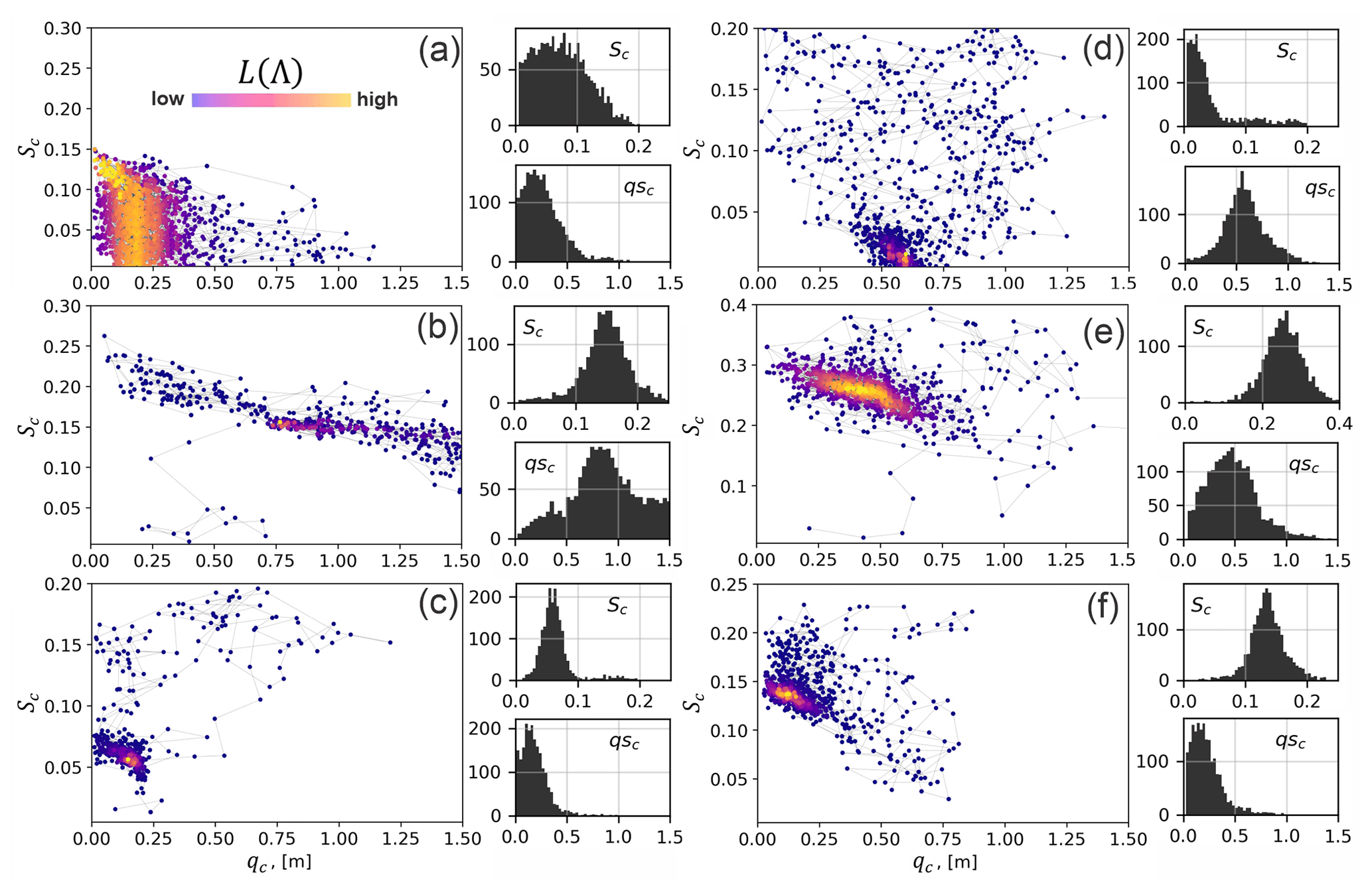
Figure 7 MWR calibration results for (a) Cascade Mountains 2009, (b) Cascade Mountains 2022, (c) Black Hills south, (d) Black Hills north, (e) Rocky Mountains, and (f) Olympic Mountains. Each result shows a scatter plot of the sampled S_c and q_c values, colored by their relative L(Λ) value. The line between points indicates the jump direction. Note that the y-axis scale differs between plots. To the right of each scatter plot are histograms of the iterated S_c and q_c parameters, which can be normalized to represent an empirical, posterior PDF of the possible S_c and q_c values that calibrate MWR to the site. The histogram y axis is the count and the x axis is S_c or q_c, as indicated on the histogram.

Profile plots of modeled Q_s and maps of the modeled planimetric runout extent, colored to indicate where the runout matched (α), overestimated (β), or underestimated (γ) the observed runout, are shown in Fig. 8. Values of Ω_T we obtained with MWR are comparable to or higher than reported values of Ω_T in the literature that used a variety of models (Gorr et al., 2022; Barnhart et al., 2021; note that to compare Ω_T values to those studies, subtract 1 from values reported in this study). Across the sites, the volumetric error of the model, Δη_E, ranges between 6 % and 15 % (median 9.1 %) of the total mobilized volume. An overall <10 % volumetric error is reasonable considering the low number of parameters required to calibrate MWR and that empirical estimates of total mobilized volume used to run other runout models can vary by as much as an order of magnitude (e.g., Gartner et al., 2014; Barnhart et al., 2021). Model performance in predicting cumulative sediment transport along the runout profile was within similar error ranges. Except for the Rocky Mountains site where MWR consistently modeled wider-than-observed flow, the mean cumulative sediment transport error along the runout profile ($Q_{{\mathrm{s}}_{\mathrm{E}}}$) was limited to between 5 % and 19 % of the mean cumulative flow determined from the observed DoD.

MWR generally successfully replicates observed sediment transport along the runout path via model parameterizations that are unique to each landslide. For example, the profile plots of Q_s at the Cascade Mountains site (Fig. 8a and b) show that during the 2009 landslide, all of the runout material flowed past the first 750 m of the runout path. During the 2022 landslide, material began to deposit just downslope of the initial landslide source area, as both observed Q_s and modeled Q_s reverse slope, indicating a decrease in cumulative flow. Model comparisons in the Cascade Mountains site were limited to the upper 750 m of the hillslope because a large portion of the runout material was lost to fluvial erosion in the valley (see the Supplement).

Figure 8 Calibrated model performance as indicated by maps of modeled runout extent, profile plots of observed and modeled cumulative sediment transport along the centerline of the runout path (Q_s; see Eq. 27), and reported values of Ω_T, Δη_E, and $Q_{{\mathrm{s}}_{\mathrm{E}}}$. The y-axis label for profile plots of Q_s is indicated. In all maps, up is north, except in (e), where north is towards the left. (a) Cascade Mountains, 2009; (b) Cascade Mountains, 2022; (c) Black Hills, north; (d) Black Hills, south; (e) Rocky Mountains; (f) Olympic Mountains.

MWR also successfully replicates the observed sediment transport patterns at the Olympic Mountains site (profile plot of Q_s in Fig. 8f) and to a lesser degree the Rocky Mountains site (Fig. 8e). This finding is notable because at the Olympic Mountains and Rocky Mountains sites, observed runout extent and sediment depositional patterns were heavily impacted by woody debris or standing trees (see the Supplement).

Using a fixed grid size of 10 m might have impacted model performance in some areas like the Olympic Mountains and Cascade Mountains 2022 sites where MWR tended to overestimate the runout width (yellow zones in Fig. 8f and b). While a 10 m DEM is generally accepted as a good balance between model detail and computational limitations (e.g., Horton et al., 2013), for small landslides, the 10 m grid was close to the width of the channels that controlled observed runout (see Fig. 1d) and may not have accurately represented the terrain. Thus, modeled flow was less topographically constrained and tended to flow over a wider area than observed.

Also, because MWR does not have an explicit representation of flow momentum, it may show poor performance in regions of the runout path where flow momentum is the primary control on runout extent. For example, for the Cascade Mountains 2009 slide, MWR underestimates a short section of slope-perpendicular flow over a bench. Review of model behavior for this slide (Fig. 9) shows how MWR successfully mimics diverging flow around a broad ridge upslope of the bench (iteration t=28 in Fig. 9) but afterwards continues to follow topographic slope and converges too rapidly into a narrow ravine along the west edge of the bench (iteration t=40 in Fig. 9; compare to runout scar in the air photo and underestimated region on the topographic bench in Fig. 8a).

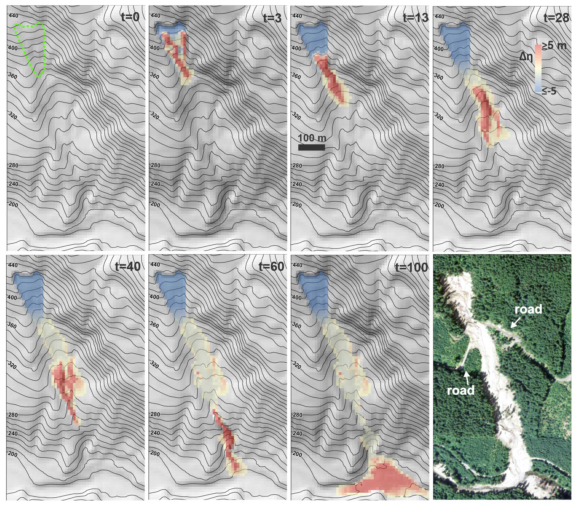
Figure 9 Illustration of modeled runout of the Cascade Mountains 2009 landslide beginning from the initial movement of the landslide body to final deposition in the river valley that demonstrates MWR response to topography. Note how the landslide slip surface directs the initial flow. Topography lines reflect the underlying terrain, which is updated after each iteration. The air photo in the last panel shows observed runout extent. Note that the upper road is not part of the observed landslide runout path.

Nonetheless, overall, calibration was best for the Cascade Mountains 2009 landslide (values of Ω_T are highest and values of Δη_E and $Q_{{\mathrm{s}}_{\mathrm{E}}}$ are lowest) and poorest at the Rocky Mountains and Olympic Mountains sites (values of Ω_T are lowest and $Q_{{\mathrm{s}}_{\mathrm{E}}}$ and Δη_E are highest). At both the Rocky Mountains and Olympic Mountains sites, because we lacked repeat lidar, we created the DoD from a map of field-estimated erosion and deposition depths and estimated the pre-event DEM. The lower calibration scores may indicate that field-estimated DoDs were not as accurate as those determined via lidar differencing. Another source of uncertainty that we have not addressed in our study is regolith thickness. At most sites, we used a uniform thickness. As regolith thickness limits maximum erosion depth (i.e., Eq. 10), using a spatially accurate regolith thickness may improve model performance. Finally, except for the Rocky Mountains site, where topography was unusually planar and the model seemed to consistently overestimate flow width, at most sites, MWR does not appear to have a strong systematic bias in modeled output, which suggests that when applied to convergent terrain, MWR may not have any structural weaknesses. In the next section, we evaluate model performance relative to runout path topography.

5.4 Runout path topography and model performance

Model behavior at the Rocky Mountains site suggests that MWR performance may systematically vary with topography (e.g., it may not perform as well on planar hillslopes). To check for systematic model variation, we compared model performance with three topographic indices described by Chen and Yu (2011). The indices are computed from the terrain in the observed runout extent and include the relief ratio ($H/L$), mean total curvature (κ), and mean specific stream power index (SPI). The index $H/L$ equals the average slope of the runout path (or relative relief), determined as the total topographic relief of the runout (measured from the center of the initial landslide to the end of the runout path) divided by the horizontal length of the runout, and indicates the mobility of the runout. The index κ represents topographic convergence, which is the second derivative of the terrain surface, with increasingly positive values of the index κ reflecting growing topographic convergence and a concave-up channel profile (e.g., Istanbulluoglu et al., 2008). The index SPI is determined as the natural log of the product of the contributing area and slope. Indices κ and SPI are computed at each node in the runout extent and model performance is compared to the mean value.

Comparison of model performance with respect to the topographic indices in Fig. 10 shows slightly improved model performance over runout paths that are less convergent (lower SPI and κ values) and on steeper terrain (higher $H/L$), but neither trend is significant. The latter finding appears to be mostly a result of how well modeled sediment transport and topographic change ($Q_{{\mathrm{s}}_{\mathrm{E}}}$ and Δη_E) replicated observed change, as there does not appear to be a trend in Ω_T with $H/L$ and the two best-performing models (both Cascade Mountains landslides) had the lowest (best) $Q_{{\mathrm{s}}_{\mathrm{E}}}$ values and low Δη_E values. Both findings are likely impacted by the grid size we used to represent terrain. As noted above, at all sites we used a 10 m grid, but at some sites 10 m does not quite capture the relief of channelized topography that controlled observed runout, leading to modeled runout that was considerably wider than observed and causing low Ω_T values (this is especially true at the Olympic Mountains site; Fig. 10a, b, and c). Also, it is important to note that these indices were calculated for the extent of the observed debris flows and may not represent the topographic form that controlled the model.

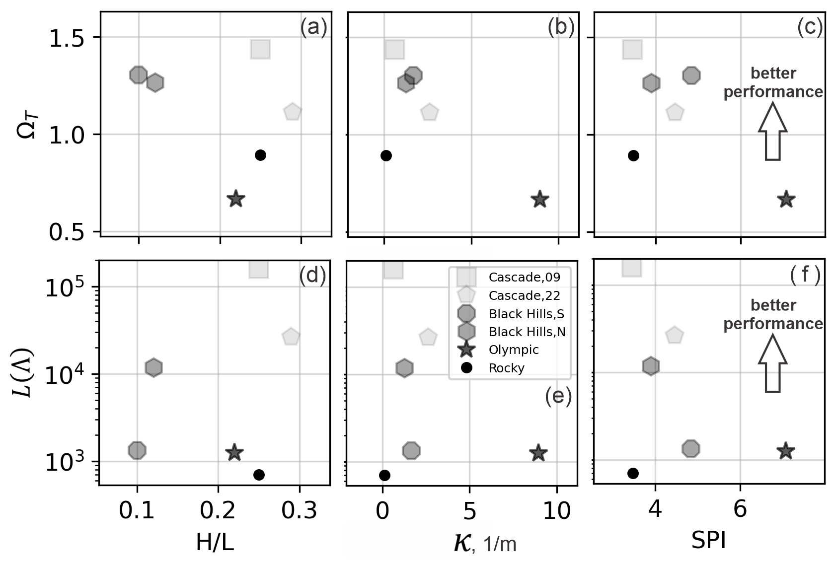
Figure 10 Illustration of model calibration, as reflected by the posterior parameter likelihood L(Λ) and planimetric fit (Ω_T) relative to topographic indices. There is no strong trend between the topographic indices and calibration performance. Note that the curvature values are scaled by a factor of 100.

In summary, using the calibration utility, we showed how MWR can be calibrated to a range of different landslide types and runout terrains. To a certain degree, though calibration, MWR can be parameterized to compensate for deficiencies in the DEM or processes not explicitly represented in the model (momentum, woody debris). While model performance at the Rocky Mountains site suggests that MWR may not perform as well on planar hillslopes, a relationship between model performance and topography was not eminent. This finding is likely a result of the contributions of numerous factors other than the terrain form, such as the DEM resolution, the quality of the DoD, the accuracy of the regolith map, and the importance of processes not explicitly included in the model that also impact performance.

6 Discussion

6.1 Strategic testing of MWR for hazard mapping applications

Having demonstrated calibrated model performance for a variety of landslides and runout terrains, we now strategically test MWR using the Cascade Mountains and Black Hills sites. Since both of these sites include two separate landslides, we can thus test model performance by swapping best-fit model parameters at each site, rerunning the models, and comparing results with the original calibrated results. At the Cascade Mountains site, the 2009 and 2022 landslides originated on the same hillslope (Fig. 8a and b). At the Black Hills site, the two landslides occurred on different hillslopes but in adjacent east–west-oriented watersheds (Fig. 8c and d).

As shown in Fig. 11, at three of the landslides (both the Cascade Mountains landslides and the Black Hills north landslide), when the best-fit parameters from the other landslide are used to predict runout, the accuracy of modeled runout planimetric extent drops but resultant Ω_T values can still be as high as or higher than values reported in other studies (compare to equivalent Ω_T values in Gorr et al., 2022, and Barnhart et al., 2021). In terms of modeled sediment transport and topographic change, swapping best-fit parameters has a more substantial effect. For the Cascade Mountains 2009 landslide, using the 2022 best-fit parameter values causes about half of the modeled runout material to be prematurely deposited on the hillslope, reducing the amount of sediment that reaches the valley floor ($Q_{{\mathrm{s}}_{\mathrm{E}}}$ increases by a factor of 9; Fig. 11). Using the Cascade Mountains 2009 parameter values on the Cascade Mountains 2022 landslide (Fig. 11b) increases modeled runout extent and results in nearly 4 times the entrainment and transport of sediment to the valley floor, causing $Q_{{\mathrm{s}}_{\mathrm{E}}}$ to increase by a factor of 20 and Δη_E by 83 %. At the Black Hills site, using the south basin best-fit model parameters at the north basin causes $Q_{{\mathrm{s}}_{\mathrm{E}}}$ and Δη_E to increase by 83 % and 39 %, respectively (Fig. 11c). Unlike the other three landslides, swapping best-fit parameters at the Black Hills south landslide results in both large sediment transport and runout extent error because the north landslide best-fit parameters applied to the south landslide causes the model to entrain too little and stop prematurely (Fig. 11d).

Figure 11 Model performance using the neighboring landslide parameter values, as indicated by maps of modeled runout extent, profile plots of Q_s, and values of Ω_T, Δη_E, and $Q_{{\mathrm{s}}_{\mathrm{E}}}$. Compare with Fig. 8. (a) Cascade Mountains, 2009; (b) Cascade Mountains, 2022; (c) Black Hills, north; (d) Black Hills, south.

As landslide hazard models often forecast hazard probabilistically, an alternative test to simply swapping the best-fit parameters is to swap parameter PDFs determined from the calibration utility and compare the probability of runout at each model node (Eq. 29). As shown in Fig. 12, similar to the first test, for three of the landslides, using the parameter distribution associated with the neighboring landslide results in relatively minor changes in model output, as indicated by where runout is more likely to occur versus not occur (probability of runout ≥50 %; Fig. 12a, b, and d), but at the Black Hills south landslide, swapping parameter PDFs causes a large change in runout probability (Fig. 12c).

Figure 12 Model tests by swapping parameter PDFs and comparing runout probability at the (a) Cascade Mountains 2009, (b) Cascade Mountains 2022, (c) Black Hills south, and (d) Black Hills north sites. (1) Runout using parameter distributions of the site and (2) runout using parameter distributions of the neighboring site.

The results of these two tests suggest that site-specific or even landslide-type-specific calibration may be needed to accurately predict runout behavior using MWR, especially when the user aims to apply MWR to sediment yield analyses and the study site consists of numerous landslide types, like the Black Hills and Cascade Mountain sites. While the need for calibration of MWR may limit model transferability across sites, this limitation holds true for most physics-based models. Barnhart et al. (2021) compared the ability of three different detailed mechanistic models to replicate an observed post-wildfire debris flow runout event in California, USA. All three models used a shallow-water-equation-based approach that conserved both mass and momentum, representing the flow as either a single-phase or double-phase fluid. All models gave comparable results in simulating the event, suggesting that there may not be a “true” best model. Despite the high level of detail and processes explicitly included in each model, all models were sensitive to and required an estimate of the total mobilized volume, and the ability to replicate observed runout ultimately depended on calibration.

We suspect that in regions where landslide processes are relatively uniform (like the Olympic Mountains site), parameterization determined through calibration to one landslide might be transferable across sites. Additionally, as noted in Sect. 3.1, we found that numerous parameter combinations allowed MWR to match observed runout extent. This finding suggests that if the project aim is limited to an evaluation of runout extent, model calibration to the site may not be as critical and parameter values from calibration to nearby landslides or even globally available repeated DEMs and air photos that show the slope of past landslide deposits (for S_c) and deposit thickness (for q_c) might be sufficient.

6.2 MassWastingRunout probability applications

In this section we briefly demonstrate how to determine runout probability from a probabilistically determined landslide hazard map or a specific, potentially unstable slope using MWR. The first application may be appropriate for watershed- to regional-scale runout hazard assessments. The second application is an example hazard assessment for a potentially unstable hillslope. Both applications are demonstrated at the Olympic Mountains site where landslide size and type tended to be relatively uniform and parameter PDFs determined through calibration may therefore represent typical runout processes in the basin.

6.2.1 Runout probability from a landslide hazard map

To determine runout probability from a landslide hazard map, we ran MWR Probability using Option 3, reading a series of mapped landslide source areas created by an externally run Monte Carlo landslide initiation model. For the landslide initiation model, we used LandslideProbability (Strauch et al., 2018), an existing component in Landlab that computes landslide probability by iteratively calculating the factor of safety (FS: ratio of the resisting to the driving forces) at each node on the raster model grid Np times from randomly selected soil (regolith) hydrology properties (e.g., soil depth, saturated hydraulic conductivity), soil strength (friction angle, cohesion), and recharge rates (precipitation input rate minus evapotranspiration and soil storage). Landslide probability at a node is defined as the number of times FS<1 divided by Np.

We first ran LandslideProbability using a 50-year precipitation event (WRCC, 2024) to determine landslide probability (Fig. 13a) over the entire Olympic Mountains model domain and create the series of Np FS maps. Details on the LandslideProbability setup are included in the Supplement. We then read the series of Np FS maps into MWR Probability, treating all nodes with FS<1 as a landslide source, and ran MWR Np times. Each iteration, MWR read a new FS map and randomly selected a new set of parameter values from S_c–q_c parameter PDFs created by the calibration utility.

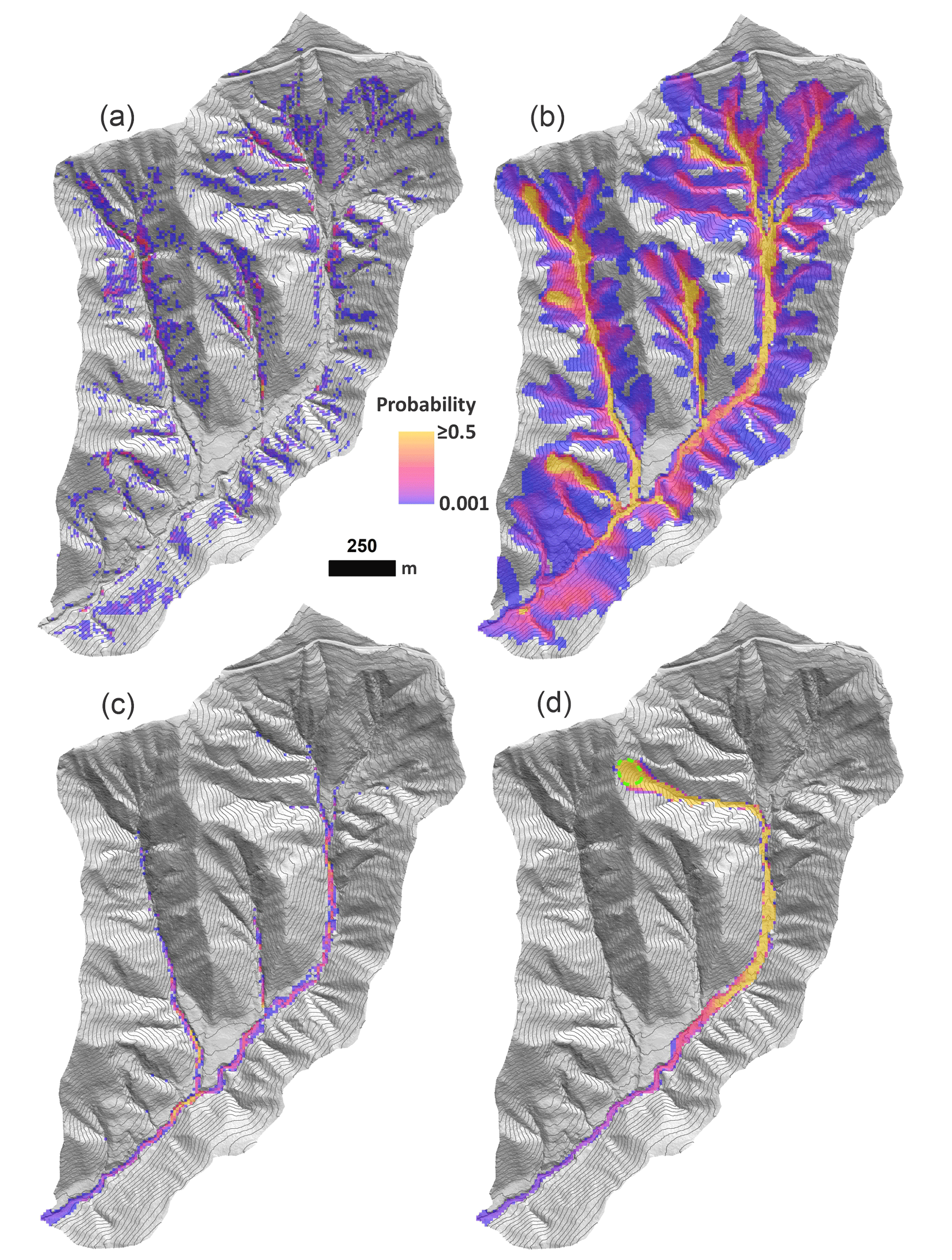
Figure 13 Olympic Mountains site. (a) Landslide probability, P(FS≤1). (b) Corresponding runout probability, P(Δη). (c) Probability of deposition greater than 1 m and (d) runout probability for the potentially unstable slope (dashed green polygon).

Runout probability, which reflects MWR parameter uncertainty (as illustrated in Fig. 7f) and uncertainty in the initial landslide size and location caused by a 50-year precipitation event, is illustrated in Fig. 13b and shows that the probability of runout is high in many of the second-order channels but low at the basin outlet. As discussed in Sect. 3, the probability of aggradation or erosion caused by the runout can be determined by adjusting the numerator of Eq. (29). As an example, the probability of deposition greater than 1 m is shown in Fig. 13c.

6.2.2 Runout probability for a specific, potentially unstable slope

When field evidence or other data indicate that a specific hillslope may be potentially unstable but the exact area of a potential landslide on that slope is unknown, MWR can be used to generate a hazard estimate that takes into account the uncertainty in the landslide area. For this application, MWR Probability is run using Option 2, which requires a polygon representing the extent of the potentially unstable slope. We designated a 0.6 ha, convergent hillslope in the headwaters of the Olympic Mountains site as a potentially unstable slope (Fig. 13d). For each model repetition, a landslide area can form anywhere within the potentially unstable slope and is at least as large as a user-defined minimum size but no larger than the potentially unstable slope. This example shows that, given uncertainty in the landslide size and location and uncertainty in MWR parameterization, if a landslide were to initiate on the potentially unstable slope, the probability of the runout reaching the basin outlet is less than 5 %.

7 Concluding remarks

In this study, we described, calibrated, and tested MassWastingRunout (MWR), a new cellular-automaton landslide runout model that combines the functionality of simple runout algorithms used in WSMs (landscape evolution and watershed sediment yield models) with the predictive detail typical of runout models used for landslide inundation hazard mapping. MWR is implemented in Python as a component for the Landlab earth surface modeling toolkit and is designed for WSM and probabilistic landslide hazard assessment applications. MWR includes a Markov chain Monte Carlo calibration utility that determines the best-fit parameter values for a site as well as empirical probability density functions (PDFs) of the parameter values. MWR also includes a utility called MWR Probability that takes the PDF output from the calibration utility to determine runout probability.

Given a DEM and map of approximate regolith depth, MWR needs only the location and geometry of an initial landslide source area to model the entire runout process. Results indicate that despite its simple conceptualization, MWR shows skill in modeling the final runout extent, sediment transport, and topographic change associated with a landslide. When compared to other models capable of replicating observed landslide inundation patterns, the strength of MWR lies in its use of field-inferable parameters, its ability to internally estimate the total mobilized volume (initial landslide body + erosion volume), and its relatively parsimonious model design.

MWR can be calibrated to a site using just two parameters (critical slope, S_c, and a threshold flux for deposition, q_c) and the MWR calibration utility enables the user to calibrate the model for a watershed within several hours on a standard desktop (Sect. 5.3). Although the predictive power of MWR hinges on calibration – a common requirement for mechanistic models – its reliance on two calibration parameters serves to constrain model uncertainty. Site-specific calibration may be needed when MWR is used for sediment yield analysis, but if the aim is limited to mapping runout extent, it may be possible to infer parameterization from nearby landslides or possibly from globally available repeated DEMs and air photos that show where past mass-wasting flows have stopped (for S_c) and how thick their frontal lobes are at the point of deposition (for q_c). Nonetheless, as a rule-based, cellular-automaton model, MWR is not designed to accurately simulate flow depth. For accurate flow depths or debris flow impact forces, a detailed mechanistic modeling approach should be used.

MWR shows a rich set of intuitive responses to topographic curvature and slope (Sect. 4). When calibrated to the runout of six different observed landslides, the volumetric error of MWR, Δη_E, ranged between 6 % and 15 % (median 9.1 %) of the observed total mobilized volume. Except for the Rocky Mountains site where MWR consistently modeled wider-than-observed flow, the cumulative flow error along the runout profile ($Q_{{\mathrm{s}}_{\mathrm{E}}}$) was limited to 5 %–19 % of the mean cumulative flow determined from the observed DEM of difference (DoD). These are considered acceptable levels of performance given that the total mobilized volume of many debris flow models assumes an order-of-magnitude range of confidence. A notable finding of this paper is that at most sites, MWR-modeled runout did not have any strong systematic bias in predictions (toward unrealistically short or wide flows, for example), which suggests that MWR is structurally sound. However, MWR may underperform compared to mechanistic models when flow momentum is the primary driver of runout extent (e.g., in areas of slope-perpendicular flow).

Finally, we briefly showed how to couple MWR with the landslide initiation model LandslideProbability to map debris flow hazard when the initial landslide location is uncertain. As a component of the Landlab earth surface modeling toolkit, MWR is designed to be compatible with other models and thus relatively easy to integrate into a WSM. An example WSM that incorporates MWR might include models for landslide initiation, hillslope diffusion, and fluvial incision to investigate the role of landslides and their runout in long-term landscape evolution. Future studies will explore large-scale application in landscape evolution or sediment yield models and characterize model parameters for different landslide types and hydroclimatic conditions. The use of a calibrated runout model in WSMs might allow for region-specific and more insightful predictions of landslide impact on landscape morphology and watershed-scale sediment dynamics.

Appendix A: Determination of k

The average erosion depth caused by the observed runout ($\stackrel{\mathrm{‾}}{E}$) can be determined from the DoD as the total erosion volume (∑EΔx²) divided by the erosion area (A_e):

$$\begin{array}{}\text{(A1)}& \stackrel{\mathrm{‾}}{E}={\displaystyle \frac{\sum E\mathrm{\Delta }{x}^{\mathrm{2}}}{A_{\mathrm{e}}}},\end{array}$$

where ∑EΔx² and A_e exclude the initial landslide body volume and area, areas of deposition (Δη>0), and areas with no change in elevation (Δη=0). In terms of the debriton conceptualization used in MWR, $\stackrel{\mathrm{‾}}{E}$ can also be written as a function of the mean number of times a debriton would need to pass over a grid cell ($\stackrel{\mathrm{‾}}{n}$) multiplied by an average erosion depth per debriton (${\stackrel{\mathrm{‾}}{h}}_{\mathrm{e}}$) to equal $\stackrel{\mathrm{‾}}{E}$ as

$$\begin{array}{}\text{(A2)}& \stackrel{\mathrm{‾}}{E}=\stackrel{\mathrm{‾}}{n}{\stackrel{\mathrm{‾}}{h}}_{\mathrm{e}}.\end{array}$$

An estimate for $\stackrel{\mathrm{‾}}{n}$ can be determined from the average length of the runout material divided by the cell width:

$$\begin{array}{}\text{(A3)}& \stackrel{\mathrm{‾}}{n}={\displaystyle \frac{l}{\mathrm{\Delta }x}}.\end{array}$$

At most sites, we approximate the average length of the runout material simply as the mapped landslide length (l). As the debritons move down slopes in excess of S_c, they entrain material, split, and spread, and the runout material tends to lengthen. Using the initial landslide length to represent the runout length thus represents a minimum value for $\stackrel{\mathrm{‾}}{n}$, and if needed, the numerator of Eq. (A3) can be multiplied by a coefficient to better match runout length. Combining Eqs. (A2) and (A3), ${\stackrel{\mathrm{‾}}{h}}_{\mathrm{e}}$ can be defined as the average erosion rate per unit length of runout debris ($\stackrel{\mathrm{‾}}{E}/l$) times the cell width:

$$\begin{array}{}\text{(A4)}& {\stackrel{\mathrm{‾}}{h}}_{\mathrm{e}}={\displaystyle \frac{\stackrel{\mathrm{‾}}{E}\mathrm{\Delta }x}{l}}.\end{array}$$

Rewriting Eq. (11) as a function of the average shear stress in the erosion-dominated reaches of the runout path ($\stackrel{\mathrm{‾}}{\mathit{\tau }}$) and assuming τ_c≅0, the debris flow erodibility parameter k can be estimated as

$$\begin{array}{}\text{(A5)}& k={\displaystyle \frac{{\stackrel{\mathrm{‾}}{h}}_{\mathrm{e}}}{{\stackrel{\mathrm{‾}}{\mathit{\tau }}}^f}}.\end{array}$$

To solve for k, we estimated $\stackrel{\mathrm{‾}}{\mathit{\tau }}$ from field-approximated debris flow depth and channel slope measurements in the erosion-dominated reaches of the runout path (Table 1). We used Eq. (13) to define $\stackrel{\mathrm{‾}}{\mathit{\tau }}$. For D_s, we used the average maximum grain size observed over the whole runout path. If τ is defined as a function of the grain-collision-dependent shear stress approach in Eq. (13) and k is determined as a function of f, as in Eq. (A5), the impact of f on model behavior is relatively small.

Appendix B

Table B1 Notation.