GraphFlood 1.0: an efficient algorithm to approximate 2D hydrodynamics for landscape evolution models

Computing hydrological fluxes at the Earth's surface is crucial for landscape evolution models, topographic analysis, and geographic information systems. However, existing formalisms, like single or multiple flow algorithms, often rely on ad hoc rules based on local topographic slope and drainage area, neglecting the physics of water flow. While more physics-oriented solutions offer accuracy (e.g. shallow-water equations), their computational costs limit their use in terms of spatial and temporal scales. In this contribution, we introduce GraphFlood, a novel and efficient iterative method for computing river depth and water discharge in 2D with a digital elevation model (DEM). Leveraging the directed acyclic graph structure of surface water flow, GraphFlood iteratively solves the 2D shallow-water equations. This algorithm aims to find the correct hydraulic surface by balancing discharge input and output over the topography. At each iteration, we employ fast-graph-theory algorithms to calculate flow accumulation on the hydraulic surface, approximating discharge input. Discharge output is then computed using the Manning flow resistance equation, similar to the River.lab model (Davy and Lague, 2009). The divergence of discharges iteratively increments flow depth until reaching a stationary state. This algorithm can also solve for flood wave propagation by approximating the input discharge function of the immediate upstream neighbours. We validate water depths obtained with the stationary solution against analytical solutions for rectangular channels and the River.lab and CAESAR-Lisflood models for natural DEMs. GraphFlood demonstrates significant computational advantages over previous hydrodynamic models, an with approximately 10-fold speed-up compared to the River.lab model (Davy and Lague, 2009). Additionally, its computational time scales slightly more than linearly with the number of cells, making it suitable for large DEMs exceeding 10⁶–10⁸ cells. We demonstrate the versatility of GraphFlood by integrating realistic hydrology into various topographic and morphometric analyses, including channel width measurement, inundation pattern delineation, floodplain delineation, and the classification of hillslope, colluvial, and fluvial domains. Furthermore, we discuss its integration potential in landscape evolution models, highlighting its simplicity of implementation and computational efficiency.

1 Introduction

River dynamics encompass key processes of landscape evolution at different temporal and spatial scales. Rivers transfer sediments downstream, control the base level of hillslopes, and set the pace of denudation rates (e.g. Clubb et al., 2019). Modelling landscape evolution and the development of fluvial landforms, in particular, thus requires a sound representation of how rivers erode, transport, and deposit material. As landscape evolution models are used to simulate the dynamics of topography over 10⁵–10⁷ years and at continental scales (Salles et al., 2023), accounting for short-term processes (e.g. daily variations of discharge, flood) at local scales remains a methodological and numerical challenge. Simulating flow in open environments in two or three dimensions requires sophisticated numerical methods, which are computationally demanding and which are thus mostly inappropriate for the challenge of simulating landscape evolution over geological timescales (Davy et al., 2017). Instead, a common approach to modelling water flow across landscapes consists of applying single or multiple flow algorithms (e.g. Tarboton, 1997; O'Callaghan and Mark, 1984). These techniques route water along topographic gradients towards one or multiple neighbouring pixels in a digital elevation model (DEM) and approximate discharge by drainage area weighted by precipitation rates (Adams et al., 2020). The approximation of steady flow using drainage-area-based discharge has been the cornerstone of integrating hydrodynamics in long-term erosion laws (e.g. Whipple and Tucker, 1999). This approach has the compelling advantage that it reduces flow patterns to a network of flow lines and has been widely used to establish empirical scaling laws relating drainage area to channel steepness and uplift (Wobus et al., 2006) or to unravel landscape evolution from the planform shape of river networks (Schumm et al., 2000; Willett et al., 2014). Moreover, these methods rely on efficient algorithms, which leverage graph theory to compute drainage area (e.g. Braun and Willett, 2013; Anand et al., 2020), flow across complex terrain (e.g. Barnes et al., 2014; Cordonnier et al., 2019; Barnes et al., 2021; Schwanghart and Scherler, 2017), or geomorphological metrics (e.g. Gailleton et al., 2019; Mudd et al., 2018; Grieve et al., 2018; Schwanghart et al., 2021). In particular, the single-flow-direction algorithm is thus the numerical workhorse for simulation software for landscape evolution (e.g. Hergarten, 2020; Braun and Sambridge, 1997; Willgoose et al., 1994; Campforts et al., 2017; Braun and Willett, 2013) and numerical frameworks for quantitative geomorphology (e.g. Barnhart et al., 2020; Gailleton et al., 2024; Schwanghart and Scherler, 2014; Mudd et al., 2019).

However, reducing rivers to lines in landscape evolution models may overtly simplify the dynamics and feedbacks of fluvial processes (Armitage, 2019). In fact, the response of rivers to climate variability, tectonic movements, or base-level changes is more varied than the simple propagation of a wave of vertical changes through a 1D network of lines. For example, changes in boundary conditions cause rivers to adjust their width (e.g. Dunne and Jerolmack, 2020; Baynes et al., 2022) and their planform flow pattern (e.g. Schuurman et al., 2013), both of which feed back on sediment fluxes (e.g. Davy and Lague, 2009). In addition, the past decade has seen the rising availability of high-resolution lidar-derived DEMs (< 1 m resolution). This means, however, that for a variety of geomorphological applications (e.g. Steer et al., 2022; Stammberger et al., 2024) rivers cannot be realistically represented by one-pixel-wide paths (Fig. 1d). Several recent studies demonstrate the advantages of integrating 2D hydrodynamics to inform the study of landforms, even on long timescales (Costabile et al., 2019; Costabile and Costanzo, 2021; Bernard et al., 2022). However, these methods are difficult to upscale for more generalized analysis due to their reliance on closed-source software and are not straightforward for non-specialists to adapt and reuse.

Here we present GraphFlood, a new and efficient method based on graph theory and finite differences, to fill this methodological gap and allow the efficient approximation of 2D hydrodynamics on high-resolution topography and/or in a longer-term landscape evolution model.

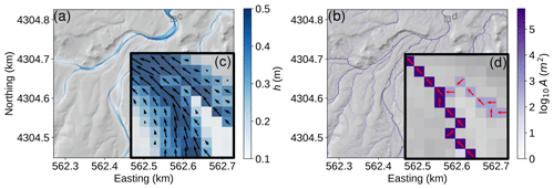
Figure 1 Comparison between water flows approximated with GraphFlood (a, c), calculating flow depth and discharge vectors, and with a classic drainage-area-based method (D8 steepest descent route) (b, d). The panels detail a channel junction and highlight how GraphFlood models flow patterns and how these differ from one-pixel-wide flows derived from the D8 algorithm. The black arrows in panel (c) represent the flow velocity vectors and are scaled to their magnitude. For panel (d), the red arrows represent the D8 flow direction. h is the flow depth and A the drainage area.

1.1 Existing solutions

A range of numerical models incorporating 2D to 3D hydrodynamics to study river systems and their morphological evolution exists, with widely different methods and levels of complexity, depending on the temporal and spatial scales of interest. Finite-element models are commonly used for reach-scale models, such as DELFT3D (Roelvink and Banning, 1995), HEC-RAS (Brunner, 2016), BASEMENT (Vanzo et al., 2021), or TELEMAC (Villaret et al., 2013). These models are designed for simulating the evolution of fluvial landforms over scales of 1–100 km and over 1–100 years and therefore fall outside the scope of this study.

Bates et al. (2010) developed a two-dimensional hydrodynamic model, Lisflood-FP, solving for the 2D shallow-water equations. Their cellular automata approach has been successfully incorporated into the landscape evolution model CAESAR Coulthard et al. (2013) to simulate reach- to catchment-scale fluvial hydro-morphodynamics (e.g. Yu and Coulthard, 2015; Liu and Coulthard, 2015; Coulthard and Van De Wiel, 2017). Lisflood-FP adopts a finite-difference scheme on the bidirectional water fluxes between pixels. While it has been applied to catchment scales over potentially thousands of years (e.g. Liu and Coulthard, 2017), its potential for longer-term and larger-scale studies remains hampered by the physics behind, which explicitly and gradually transfer water from one cell to another. Specifically, any upstream change in runoff input (e.g. precipitation) must be gradually propagated downstream one pixel per computational time step. Although modelling non-steady flows is crucial for simulating transient responses to individual storm events (e.g. Van De Wiel and Coulthard, 2010), it becomes a limiting factor when simulating over longer timescales or larger scales. Bates et al. (2010) and subsequent improvements by de Almeida et al. (2012) have been utilized in other landscape evolution frameworks (e.g. Barnhart et al., 2020) following the same principle.

An alternative approach is to focus on the stationary state of the river network (i.e. in equilibrium with the input field of runoff). The main challenge in efficiently estimating the stationary solution lies in spreading the flow to its equilibrium field. The latter depends on the final geometry of the hydraulic surface, which cannot be deduced from the geometry of the terrain alone. To address this point, Davy et al. (2017) developed an efficient particle-based solution to solve the shallow-water equations. In this approach, precipitons (i.e. elementary volumes of water) are released onto the landscape. Each precipiton follows a stochastic path down the hydraulic surface, increasing the flow depth by a constant value, representing the total water influx. This increase is balanced by a decrease in flow depth, calculated using Manning's equations and where each precipiton has its own timestamp. The frequency at which precipitons pass through a cell determines the final, stationary flow depth field. This method is computationally efficient in areas where flow converges and a high frequency of precipitons passes through (e.g. fluvial valleys). However, the efficiency and accuracy of River.lab (formerly FLOODOS) depend on the frequency of precipiton passage. Accurately approximating the shallow-water equation becomes challenging in regions with lower drainage areas or any domains where the frequency of precipiton passage is very low (e.g. flat areas, hilltops, hillslopes, smaller tributaries). This behaviour is accentuated in large DEMs, where the probability of precipiton passage is even lower.

Finally, Pelletier (2008) outlined the prototype of a highly iterative solution that repeatedly runs a multiple-flow-direction flow-routing DEM (e.g. Tarboton, 1997). This process incrementally and arbitrarily increases the flow height until satisfying an equilibrium between flow depth and input discharge. However, it requires a significant number of iterations to ensure all the cells have converged to the final result.

1.2 A new solution based on graph theory

In this contribution, we introduce GraphFlood, a novel iterative approach that is both efficient and adaptable for solving the shallow-water equations across entire landscapes. Numerically, each DEM location is linked to its neighbours through unique directional connections, either upstream or downstream. In graph theory, this structure is known as a directed acyclic graph, which allows for the application of efficient algorithms for information propagation through landscapes (e.g. Anand et al., 2020; Braun and Willett, 2013; Gailleton et al., 2024; Hergarten and Neugebauer, 2001). Similar to Davy et al. (2017), GraphFlood assumes steady flow to focus on the stationary solution, meaning that flow is propagated across the landscape instantaneously. However, unlike Davy et al. (2017), whose accuracy and efficiency vary depending on the frequency of passage of discrete particles, GraphFlood leverages the graph structure to process the entire landscape in each iteration. This includes domains with low drainage areas. Runoff is propagated using drainage area weighted by precipitation rates, and local discharge is calculated using Manning's friction equations. At each iteration, the balance of input and output discharges is incrementally adjusted for every cell in the landscape, refining the flow depth until hydraulic equilibrium is achieved. This global approach is scalable and allows for targeting larger DEMs without compromising the efficiency or accuracy of the algorithm.

In the following sections, we first describe the theory behind our method, then explain the algorithm and the associated finite-difference scheme. We then test different case studies to demonstrate the method's potential for flood modelling, morphometric analysis, and landscape evolution modelling. Finally, we discuss the limitations and potential future developments of the model.

2 Theoretical background

First, we outline the governing equations behind GraphFlood. We use the 2D shallow-water equations to approximate the physics of water flow in open environments. They integrate the three-dimensional Navier–Stokes equations over the vertical dimension, assuming that the velocity field varies primarily in the horizontal direction. Different variants of the shallow-water equations are commonly used to model flooding beyond reach scale (e.g. Bates et al., 2010; de Almeida et al., 2012; Davy et al., 2017; Bates, 2022). The 2D shallow-water equations consist of a mass conservation equation and a momentum conservation equation. Using the notation of Davy et al. (2017), the mass conservation equation can be written as

$$\begin{array}{}\text{(1)}& {\displaystyle \frac{\partial h}{\partial t}}-\mathrm{\nabla }\cdot \left(\mathit{q}\right)=\mathrm{0},\end{array}$$

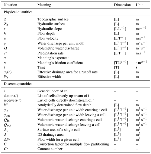
where h is the water depth [L], t the time [T], and q the discharge per unit width [L² T⁻¹].

Neglecting inertia, Manning et al. (1895) demonstrated that the momentum equation can be simplified into Manning's equations where flow velocity u (in L T⁻¹) is expressed as

$$\begin{array}{}\text{(2)}& \mathit{u}={\displaystyle \frac{h^{\mathit{\alpha }}}{n}}{\displaystyle \frac{\mathit{s}}{\Vert \mathit{s}{\Vert }^{\frac{\mathrm{1}}{\mathrm{2}}}}},\end{array}$$

where α is Manning's exponent, usually assumed to equal $\frac{\mathrm{2}}{\mathrm{3}}$, n is Manning's friction coefficient, and s is the steepest gradient of the hydraulic surface. The hydraulic surface is $Z_{\mathrm{h}}=Z+h$, the elevation of the flow depth h on the top of the topographic surface Z.

In order to insert Eq. (2) into Eq. (1), discharge per unit width and velocity are related via flow depth.

$$\begin{array}{}\text{(3)}& \mathit{q}=\mathit{u}\cdot h\end{array}$$

Unlike similar methods (e.g. Bates et al., 2010) or more sophisticated formulations (e.g. Brunner, 2016) incorporating additional physical elements (e.g. inertia, turbulence), our method is designed to be optimized when these components can be neglected (Davy et al., 2017). We use Q to refer to the volumetric flux [L³ T⁻¹] and the subscript Q_in and Q_out to respectively refer to quantities entering or leaving a given cell.

These equations can simulate the propagation of water through space and time dynamically, solving a transient flood wave. ∇⋅q is the difference between q_in made of q_out from upstream neighbours and q_out from the current cell to its downstream neighbours. For a constant input of q_in on a landscape (e.g. constant precipitation rates, fixed input discharge), the system has an equilibrium state – or stationary solution – where the water depth and hydraulic slope lead to a q_out balancing q_in. The total Q_in for the stationary state for a given location becomes the integration of all the source terms (e.g. precipitation, resurgence) over the drainage area upstream of a given location.

In this contribution, we refer to the transient solution when we seek to solve the transient propagation of Q through space and time and to the stationary solution when we are only interested in the equilibrated fields.

3 A graph-based iterative method

We present a numerical framework to solve the governing equations outlined in Sect. 2. Our scheme applies various variants of an explicit finite-difference method on a directed acyclic graph (see Braun and Willett, 2013; Barnhart et al., 2020; Gailleton et al., 2024, for other geomorphological models using this family of methods). It aims to provide efficient solutions, suitable for large-scale DEMs and landscape evolution models. Our iterative scheme is optimized for the stationary solution but can be used for transient simulation. In the following, we detail the numerical graph structure required by our method, describe the finite-difference scheme, explain the transient and stationary solutions, and validate them against analytical solutions.

3.1 Numerical structure

We use the following terms adopted from graph theory (see  Heckmann et al., 2015, for a comprehensive review of the use of graph theory applied to geomorphological applications): a discrete location is represented by a node, linked to its neighbour nodes via links. The links are directed edges linking donors to their downstream receivers. In our reference donors have a higher hydraulic surface (Z+h) than their receivers. The algorithm is compatible with any type of grid (e.g. hexagonal grid or triangular network), as long as the directed acyclic graph structure defines the topology between the pixels or facets. Each link is characterized by a specific length ∂l representing the distance between the two neighbour nodes and a link width ∂w representing the local width. Each node represents a cell area A_c ([L²]). The scheme also requires common directed acyclic graph algorithms: topological ordering, which provides a list of nodes sorted from upstream to downstream, and sink filling, a method for filling local minima disconnected from the rest of the graph (e.g. lakes, local noise). The directed acyclic graph can utilize either a single-flow-direction topology (Braun and Willett, 2013), where each node has a single receiver (e.g. steepest descent or D8), or a multiple-flow-direction directed acyclic graph where each node is linked to multiple receivers (e.g. Tarboton, 1997; Anand et al., 2020). This distinction is important because operations on single-flow-direction directed acyclic graphs are generally simpler and more efficient than those on multiple-flow-direction directed acyclic graphs (e.g. Braun and Willett, 2013; Anand et al., 2020). However, it is worth noting that the latter captures more details about flow topology and tends to increase the accuracy of the represented processes (e.g. Armitage, 2019).

In this contribution, we developed the method for regular grids. In the stationary case, we use the algorithms of Barnes et al. (2014) and Cordonnier et al. (2019) to ensure flow continuity and proceed to an initial filling of the local minima (e.g. noise, lake). Topological sorting operations use a modified version of Braun and Willett (2013) for a single flow direction and a variant of Anand et al. (2020) for multiple flow directions. These modifications involve minor data structure changes that enhance performance and readability without altering overall functioning (see Gailleton et al., 2024, for detailed implementations). One advantage of GraphFlood is that it can be implemented using existing computational frameworks for DEM analysis and landscape evolution model (LEM) simulation (e.g. Schwanghart and Scherler, 2014; Gailleton and Mudd, 2021; Barnhart et al., 2020): the base of the algorithm only needs to calculate flow direction and topological order. A notable difference compared to existing frameworks is that we calculate the directed acyclic graph using the hydraulic surface rather than the topography.

3.2 Iterative explicit finite-difference scheme

We use an explicit finite-difference scheme to solve Eq. (1). In the transient case, the numerical solution predicts flow depth change for every node i:

$$\begin{array}{}\text{(4)}& {\displaystyle \frac{h_i^{t+\mathrm{1}}-h_i^t}{\mathrm{\Delta }t}}={\displaystyle \frac{\sum _{d=\mathrm{donors}\left(i\right)}{Q}_{{\mathrm{in}}_d}-\sum _{r=\mathrm{receivers}\left(i\right)}{Q}_{{\mathrm{out}}_r}}{A_{\mathrm{c}}}},\end{array}$$

where $Q_{{\mathrm{in}}_d}$ represents the discharge from a donor d to the node i and $Q_{{\mathrm{out}}_r}$ the discharge from the node i and a receiver r. For the latter, in the case of a single flow direction (i.e. single receiver), Eq. (3) becomes

$$\begin{array}{}\text{(5)}& Q_{{\mathrm{out}}_i}={\displaystyle \frac{\mathrm{\Delta }W}{n}}{h}_i^{\mathit{\alpha }}\sqrt{s_{ir}},\end{array}$$

where i and r are a given node and its single receiver, respectively, and ΔW is the flow width ([L]) in the given direction. Because flow can only go through one link, ΔW is easy to determine. For example, for our case of a regular grid, it is Δx in the y direction, Δy in the x direction, and the diagonal length for the other cases. As noted by Coulthard et al. (2013), multiple flow directions can become increasingly more complicated: multiple receivers mean ΔW “overlaps” and using the direct width of flow for each link can break the conservation of mass. Let us imagine a regular grid considering D8 neighbouring (cardinal and diagonal directions): a node that would discharge to all these directions would integrate twice the total flow width. Porting this formulation to multiple flow directions requires a correction factor. Equation (3) in a multiple-flow-direction directed acyclic graph therefore becomes

$$\begin{array}{}\text{(6)}& Q_{{\mathrm{out}}_i}={\displaystyle \frac{C}{n}}{h}_i^{\mathit{\alpha }}{\displaystyle \frac{\sum _{j\mathrm{in}\mathrm{receivers}}{s}_{i,j}\mathrm{\Delta }{W}_{i,j}}{\sqrt{s_{i,j,\max }}}},\end{array}$$

where $s_{i,j,\max }$ is the hydraulic slope in the direction of maximum descent.

By definition, and for a given flow depth, both single-flow-direction and multiple-flow-direction discharges should be equal. Therefore, the correction factor is

$$\begin{array}{}\text{(7)}& C={\displaystyle \frac{s_{i,j\max }\mathrm{\Delta }{W}_{i,j\max }}{\sum _{j\mathrm{in}\mathrm{receivers}}{S}_{i,j}\mathrm{\Delta }{W}_{i,j}}},\end{array}$$

Eq. (6) is then equivalent to Eq. (5), and the difference between the two solvers only remains in the partitioning of Q_in, which becomes proportional to $s_{i,j}\mathrm{\Delta }{W}_{i,j}$.

Both transient and stationary solutions follow that scheme to calculate the output discharge; the difference is the calculation Q_in for all nodes. The overall process is outlined in Algorithm 1.

Algorithm 1 Iterative stationary solver.

Initialize directed acyclic graph structure on hydraulic surface

while Convergence criterion (see Sect. 3.3 and 3.4) not met do

Update directed acyclic graph with hydraulic surface

for each node n in downstream topological order do

Calculate s(n) and weight partitioning

Determine Q_in(n) from upstream nodes

Calculate Q_out(n)

Transfer Q to receivers of n

end for

Increment h_w for all nodes

end while

3.3 Transient solution

For the transient solution, $Q_{{\mathrm{in}}_{di}}$ is $Q_{{\mathrm{out}}_{di}}$ calculated between the donor and this node plus an eventual local external Q_in source term (e.g. resurgence, precipitation, grid edge input). The method becomes similar to Bates et al. (2010) – but their formulation includes an approximation of inertia and has a D4 flow topology. Although straightforward and massively parallelizable (e.g. Apel et al., 2022), this method does not benefit from the directed acyclic graph data structure as signals are propagated from one node to their immediate neighbours. If external Q_in is kept constant long enough, this solution converges toward a unique equilibrium stationary state and is not efficient if the intermediate transient steps are not important.

Like any explicit finite-difference methods, higher time steps lead to fewer iterations and more efficient spread but also more instability. Equation (2) expresses the velocity of a flood wave and therefore its stability can be approximated using the Courant–Friedrichs–Levy (CFL) conditions:

$$\begin{array}{}\text{(8)}& Cr=\mathrm{\Delta }t{\displaystyle \frac{u_{\max }}{\mathrm{\Delta }{x}_{\max }}},\end{array}$$

where Cr is the Courant number.

The transient solution converges toward an equilibrium hydraulic surface and Q field. We estimate convergence based on median h and $\frac{\mathrm{\Delta }h}{\mathrm{\Delta }t}$ for the whole landscape. We stop the iterative process once the first plateaus and when the increment in flow depth becomes lower than an acceptable ad hoc threshold (e.g. 10⁻⁹ m).

3.4 Stationary solution

The stationary solution optimizes convergence towards the equilibrated solution – i.e. the steady-state flow depth and discharge fields to an input runoff. Ultimately, the amount of water flowing through a landscape equates to the runoff rate propagated into the drainage network. Numerically speaking, it results in calculating a weighted drainage area, a procedure already in use in GIS applications and LEMs when it comes to integrating the effect of spatial variations in precipitation (e.g. Leonard et al., 2023). In the case of effective precipitation, each node receives a local P(x,y)ΔxΔy. In reach mode, the model receives Q_in in the boundary cells corresponding to the upstream section of the river. In both cases, received water is then recursively transferred to all the downstream nodes following the topological order. It effectively reduces the need to propagate a signal gradually from upstream to downstream one node at a time. However, the final hydraulic surface being different than the topographic surface, the algorithm needs to iterate to gradually build the hydraulic surface. From the first iteration, discharge is propagated through the full landscape and starts “piling up” h on the whole flow path. Every iteration recomputes the directed acyclic graphs from the updated hydraulic surface, effectively spreading Q_in towards its final geometry balanced by Q_out. The time step in the stationary mode is a numerical stability criterion modulating the magnitude of flow depth increment. Similarly to the transient solution, we estimate convergence based on median h and Δh between each iteration for the whole landscape and consider convergence reached once median $\mathrm{\Delta }h<\mathrm{1}\times {\mathrm{10}}^{-\mathrm{9}}$ m.

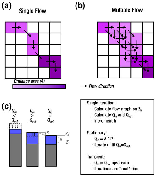
Figure 2 Graphical representation of a single iteration with GraphFlood. Panels (a) and (b) show the flow routing structuring the graph for a single flow direction and multiple flow directions, respectively, in map view. Note that this figure only displays flow routing from a single source for clarity. Panel (c) illustrates in cross-sectional view the increment or decrement of flow depth at the end of the iteration depending on calculated or propagated discharges.

3.5 Validation

We validate the numerical scheme against an analytical solution (Fig. 3) using a rectangular channel (Bates et al., 2010; Davy et al., 2017). We combine Eqs. (1) and (3) to obtain an analytical stationary flow depth denoted h^*.

$$\begin{array}{}\text{(9)}& h^{*}={{\displaystyle \frac{n{Q}_{\mathrm{in}}}{\mathrm{d}x\sqrt{\mathit{s}}}}}^{\frac{\mathrm{1}}{\mathit{\alpha }}}\end{array}$$

Equation (2) predicts that in the case of a rectangular channel with a constant given slope S₀, the slope of the stationary water surface s should be equal to S₀. Assuming a boundary condition of fixed hydraulic slope, we can calculate a reference h^*.

We run GraphFlood with the transient and stationary solvers as well as multiple-flow-direction and single-flow-direction schemes on a 200 m × 40 m rectangular channel with a regular dx=1 m (more details in the Fig. 3 caption). Figure 3a shows the results for all runs. Each simulation converges towards h^*, validating the numerical methods. The number of iterations to reach h^* – directly linked to the computational efficiency of the algorithms – is significantly higher for the transient model as it needs to propagate the flood wave through the whole channel one node per iteration. This behaviour is likely to worsen with the complexity of a natural river network where any junction would need catchment-wise upstream information before being equilibrated and being able to propagate a signal downstream. Figure 3b zooms in on the stationary models that reach a stationary state in about 300–1000 iterations, roughly 400 times faster than the transient model. Adaptive time stepping based on the CFL condition slightly reduces the number of iterations required to reach the analytical solution, and the single-flow-direction model converges in fewer iterations than the multiple-flow-direction model.

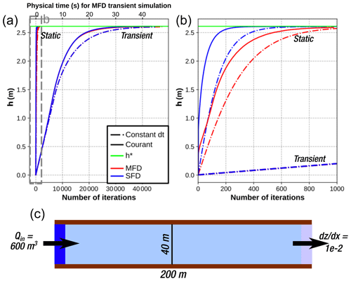
Figure 3 Validation tests for the multiple-flow-direction and single-flow-direction stationary and transient simulation for a given Q_in=15 m³ s⁻¹. The scenarios with constant dt were set to $\mathrm{1}\times {\mathrm{10}}^{-\mathrm{3}}$ s, and the scenarios with the CFL condition were calculated with $Cr=\mathrm{3}\times {\mathrm{10}}^{-\mathrm{3}}$. Both were chosen empirically as values balancing model performance and stability of the final results. Panel (a) displays the full results for all the simulations, while panel (b) zooms in on the stationary model results. Panel (c) describes the model setting in map view. A total of 1000 iterations of GraphFlood on this small rectangular channel take about 0.7 s for a single flow direction and 1.2 s for multiple flow directions with a CPU Intel i9-11950H.

3.6 Test sites

We test GraphFlood on two lidar-derived DEMs and aim to explore the effect of different geographical contexts on the algorithm in terms of both relief and climate. Our first test site is located near Green River (Utah, USA), a low-relief area in an arid context with smooth hillslopes. The second test site is the Hanalei River catchment in Hawaii (USA), with sharp relief made of volcanic rocks, steep hillslopes, and entrenched valleys. The original spatial resolution of both DEMs is 1 m, provided pre-processed from point clouds and provided by https://www.opentopography.org (OpenTopography, 2020, 2012). We also down-sample the DEM of the Hanalei River catchment to a resolution of 5 m using a cubic resampling implemented by GDAL/OGR contributors (2023) to process a larger watershed and test GraphFlood at multiple resolutions.

4 Results

4.1 Numerical behaviour for a single simulation

We first explore the behaviour of the model during a single simulation, where we run the multiple-flow-direction stationary algorithm for both test sites for a high-intensity rainfall rate of 100 mm h⁻¹. We deliberately chose an extreme rainfall rate to test the algorithm under high-flow conditions during which multiple diverging river channels are activated.

We run the model to convergence (Fig. 4 – see caption for the full simulation parameters). In terms of channel network topology, GraphFlood is able to reproduce diverging and converging flow patterns that follow converging and diverging channel networks. This behaviour is striking on Green River, where the broad valleys consist of an interwoven network of channels, but also well-captured on the clearer channel beds of Hanalei. GraphFlood in that way contrasts with drainage-area-based flow patterns which by nature converge toward a single line of flow (e.g. Fig. 1). In both cases the majority of the DEM pixels display insignificant flow depth (< 1 cm) as one should expecting from natural landscapes where rivers only represent small portions of the landscape.

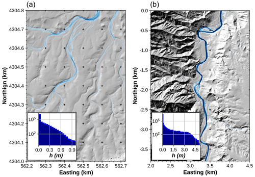
Figure 4 Flow depth field calculated with GraphFlood for fluvial valleys in Green River, Wyoming, USA (a), and Hanalei, Hawaii, USA (b). The maps are zoomed in on major fluvial valleys for clarity. Both histograms show the distribution of water height for the multiple-flow-direction stationary solutions calculated during a high storm event (precipitation rate 100 mm h⁻¹). Note the logarithmic y scale on the histogram demonstrating that the majority of points have low flow depth (< 1 cm).

GraphFlood reaches convergence in 4000 and 3000 numerical iterations for the Green River and Hanalei (Fig. 5a and b), respectively, based on the criterion outlined in Sect. 3.3 and 3.4. At first glance, this number is high, but we observe a discrepancy in the spatial and temporal patterns of convergence. The model converges asymptotically in the fluvial domain only where fewer than 200 iterations for Green River and fewer than 60 for Hanalei are enough, as illustrated by the striking spatial variations in Fig. 5c and d. Low drainage area on the hillslopes induces lower increments of flow depth, which combined with high slopes explains the slower convergence on the hillslopes.

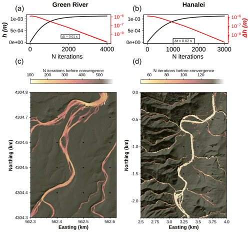
Figure 5 Rate of convergence for the simulation in Fig. 4 with $\mathrm{\Delta }t=\mathrm{1}\times {\mathrm{10}}^{-\mathrm{2}}$ and $\mathrm{\Delta }t=\mathrm{2}\times {\mathrm{10}}^{-\mathrm{2}}$ s. In panels (a) and (b), we show in black the median flow depth function of the number of numerical iterations and in red the changes in flow depth between each iteration. Panels (c) and (d) demonstrate the spatial variability in the rate of convergence. Note that GraphFlood converges significantly faster in the fluvial domain. The number of iterations before convergence is defined as the first iteration reaching 95 % of its equilibrium value.

We test the sensitivity of the model to its numerical parameter Δt and its discretization Δx. Δt controls the magnitude of the h increment. Maximizing it optimizes the spreading of Q to its equilibrium field. However, our tests also highlight that while significant overestimation provokes numerical divergence, slight overestimation converges to an underestimated final h. The spatial resolution of a DEM, Δx, can be dictated by the availability of source data, but it can be interesting to reduce the resolution of a DEM in order to process a larger area (if computing speed or memory are limiting factors). For this test, we use the Green River DEM resampled from dx = 1 m to dx = 10 m. Flow patterns remain relatively similar from one resolution to another. However, loss of detail is observed at lower resolution as expected. Lowering the resolution leads to lower hydraulic slopes on average and subsequently a decrease in Q_out and an increase in the total volume of water stored on the DEM.

We also test the sensitivity to the physical parameters. Manning's coefficient is an empirical friction parameter reflecting the local surface condition (e.g. vegetation, bed roughness; see Arcement and Schneider, 1989, for different measurements). Higher friction values predicts a higher and more distributed water surface required to reach the same Q_out. Higher input discharges or precipitation rates lead to higher flow velocity and therefore lower the stability condition, thus impacting the speed of convergence.

4.2 Comparison with existing models

We compared GraphFlood with previous models sharing similar applications (relatively large-scale and medium-term hydrology): CAESAR-Lisflood (Coulthard et al., 2013) and River.lab (formerly EROS/FLOODOS – Davy et al., 2017). We ran the three models on Green River with a constant rainfall rate of 30 mm h⁻¹ and a classical friction coefficient of 0.033. We ran the three stationary simulations, as detailed in Sect. 3.4. We compared the fields of flow depth by pairs of models (Fig. 6). Overall, the differences between the models are minimal, centred between $\mathrm{3}\times {\mathrm{10}}^{-\mathrm{4}}$ and $\mathrm{5}\times {\mathrm{10}}^{-\mathrm{4}}$ m. The differences can be linked to the differences in flow routing. CAESAR-Lisflood can only route flow to cardinal directions, and therefore the distribution of slopes is not exactly the same as GraphFlood and River.lab, which include diagonals. River.lab relies on a stack of consecutive 1D stochastic paths on a 2D grid, while GraphFlood offers a continuous solution in space and time, explaining the small differences in the final solutions.

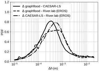
Figure 6 Benchmark comparing the difference in the stationary field of flow depth between CAESAR-Lisflood, River.lab (formerly EROS/FLOODOS), and GraphFlood. The data express the distribution of flow depth differences for each pair of models. The distributions are estimated using a kernel density estimation.

5 Applications and potential

5.1 Flood extent

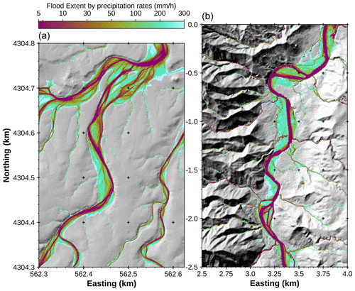
The computational efficiency of GraphFlood enables the rapid simulation of stationary flow depth and extents under different runoff intensities. We ran the model for effective precipitation rates ranging from 5 mm h⁻¹ – approximating low-flow conditions – to 300 mm h⁻¹ – extreme storm conditions. Figure 7 shows the flood extent for each different scenario on a per node basis. In addition to fast engineering application or flood risk assessment (e.g. Bates, 2022), Bernard et al. (2022) noted that flow metrics calculated from different precipitation rates could be used to determine the extent of flood plains and of the different channels of a river system. While more computationally demanding than the geometrical method (e.g. Clubb et al., 2022), GraphFlood offers a physics-based method for self-emerging the floodplain geometry. Low-flow conditions in purple in Fig. 7 emphasize the geometry of channel beds, while higher-flow storm-related conditions in blue indicate the maximum extent of the floodplain. We only computed uniform-precipitation-rate scenarios, but GraphFlood can ingest spatially variable matrices of effective precipitation if coupled with more sophisticated precipitation/infiltration data or models.

Figure 7 Flood extent at stationary solutions for different precipitation rates. The colours represent the minimum precipitation rate at which the area is flooded by at least 10 cm of water. Note the self-emergence of bedforms and floodplains.

5.2 Flood waves

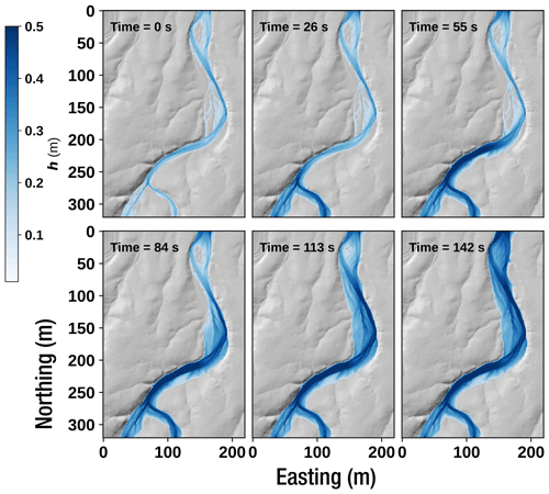
While the model is primarily designed and optimized for the stationary state, we illustrate its capabilities to model the transient propagation of a flood wave (e.g. sudden increase in input discharge in reach mode) in Fig. 8. We isolated a small section from the Green River site and started from equilibrated low-flow conditions (time 0 s). We instantly increase the input discharge by a factor of 3, and the different panels display the spatial propagation of the resulting flood wave through time.

Figure 8 Propagation of a flood wave through time using GraphFlood in transient mode. The initial conditions correspond to a steady flow for a total input of 3 m³ s⁻¹, which is triple at the start of the simulation. The times indicated in the different panels are the simulation times.

5.3 Hydromorphometry

One of the main technical challenges in topographic analysis studies is to determine from topographic data the transitions between the fluvial network, colluvial channels, and hillslopes. Such classification is useful for understanding landscape dynamics (e.g. Grieve et al., 2016; Hurst et al., 2019) to constrain geomorphological laws (e.g. Perron, 2011). Landscape evolution models also routinely apply different process laws based on that transition (e.g. Perron, 2011) or to assess the response of landscape to tectonics or climate changes (e.g. Willett, 1999). A common approach consists of isolating breaks in slope–area distributions to determine a critical drainage area value (e.g. DiBiase et al., 2010; Whipple et al., 2013). A number of geometrical/empirical methods have also been developed to isolate individual channel heads in higher-resolution DEMs (e.g. Pelletier, 2013; Clubb et al., 2014; Lurin et al., 2023). These methods' intrinsic limitation is the use of surface topography: the latter by nature cannot express the actual geometry of water bodies, making them harder to detect.

Recent studies (Costabile et al., 2019; Costabile and Costanzo, 2021; Bernard et al., 2022) have demonstrated that approaches explicitly approximating hydrodynamics effectively overcome that limitation by computing hydrology-derived geomorphological metrics from hydraulic surface and discharge. In particular, Bernard (2022) show that the slope–area relationship can incorporate hydrological information by replacing topographic slope by the hydraulic slope at equilibrium and D8 drainage area by a specific drainage area $a_{\mathrm{s}}\left(r\right)=\frac{q}{r}$, where r is the runoff precipitation rate and q the discharge per unit width. s and a_s(r) are naturally embedded within the directed acyclic graph structure of GraphFlood, allowing a more systematic and straightforward bulk computation.

First, as illustrated in Fig. 7, applying GraphFlood with high precipitation rates proves to be an efficient method for determining the extent of the floodplain. Next, we extracted s and a_s(r) for both test sites and applied thresholds based on the breaks in slope of the log a_s(r)–log s plots to delineate different domains (Fig. 9a and b). Following the approach of Bernard (2022), we isolated domains I, II, and III, which correspond to the classic geomorphological features of convex hillslopes, concave valleys, and fluvial regions, respectively.

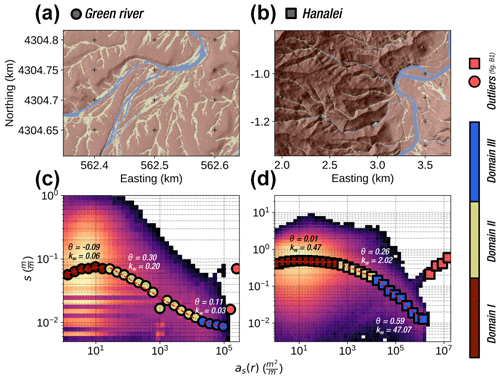
Figure 9 Classification of different domains at the test sites based on the s–a_s(r) relationship. Panels (a) and (b) show the classification of an area of interest for the Green River and Hanalei test sites, respectively. Panels (c) and (d) show the corresponding log s–log a_s(r) plots. The colour of the points corresponds to their domains. As described in the main text, we determined the separations of the domains using the breaks in slope in the binned data. Outliers, belonging to nodes showing high a_s(r) and potentially high s, are displayed in Appendix Fig. B1.

The s-a_s(r) relationships for both catchments (Fig. 9c and d) generally exhibit patterns similar to those observed in classic slope–area techniques. In domain I, s increases and then plateaus before decreasing, with breaks in slope in the log–log space defining the transitions to domains II and III (e.g. Montgomery, 2001). Notably, domains I and III define hillslopes and fluvial areas, as discussed in Bernard (2022). Domain II reveals a variety of patterns, including (i) convergent hillslopes that gradually concentrate flow into small channels and (ii) divergent branches of fluvial channels in partially flooded regions. For each domain, we calculated θ and k_w, which are equivalent to the concavity and steepness indices in Flint's law (Flint, 1974). The observed variation in θ values is greater than that typically seen in Flint's law (Gailleton et al., 2021). The significant scatter in the log s–log a_s(r) plots is consistent with common slope–area plots. However, the incorporation of hydraulic information and the reduction of topographic noise by using the hydraulic surface allow us to link local outliers to specific morphological features. For example, low s and low a_s(r) values reflect a flat surface disconnected from the active channel (e.g. a fluvial terrace), a feature that traditional methods might struggle to detect. The fluvial domains also exhibit an interesting surge in s for high a_s(r), a novel feature compared to traditional slope–area plots, decoupled from the typical monotonic downstream increase in drainage area. We isolated these outliers using the last break in slope in Fig. 9c and d and visualized some of them in Appendix Fig. B1. A few of these points represent numerical artefacts linked to local minima that artificially increase h and, consequently, the discharge and a_s(r). Most of them correspond to areas of accelerated flow and concentrated discharge where channels narrow and branches converge and potentially where hydraulic slopes increase due to topographic knickpoints.

This last observation highlights the kind of additional information the hydrology-aware approach unravels. Bernard et al. (2022) built on earlier work restricted to a hillslope (Gallant and Hutchinson, 2011), where $s\equiv \frac{\mathrm{d}z}{\mathrm{d}x}$, to develop this principle further and express a proxy for channel width, called specific width w_s(r). The specific width is calculated from the ratio between single-flow-direction drainage area (i.e. most convergent flow lines) and the specific drainage area (i.e. representing the flow field spread to its natural extent). As acknowledged by the authors, the challenge lies in the choice of the single flow path, which will determine A: if the latter does not coincide with that main discharge field, the results are highly noisy and difficult to interpret. With the precipiton method, Bernard et al. (2022) suggest the calculation should be post-processed on the discharge field calculated at low-flow conditions and following its maximum values.

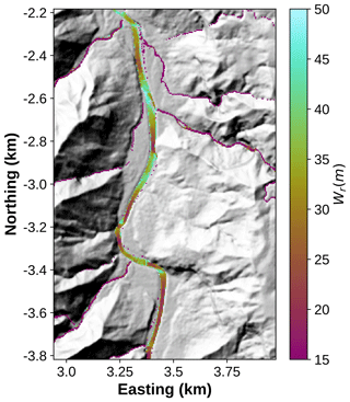
We leverage GraphFlood integrated directed acyclic graph data structure to optimize this process and generalize it to the 2D channel network. Using the directed acyclic graph calculated from the equilibrated hydraulic surface, we repeat a stochastic walk to calculate A, where the steepest receivers of each node are determined from the multiple flow receivers using the hydraulic surface and a probability function of these receivers' Q_out. Repeating this walk about 50 times and keeping track of node-wise max(w_s) ensures all the channel pixels are visited. Figure 10 displays the resulting field of flow width where we simply apply a threshold to filter out unreasonable values where A lies out of the main channel for a few nodes. This method effectively highlights fine-grained variations in flow width and allows its systematic, efficient extraction by unravelling patterns of “width” knickpoints.

Figure 10 Effective width for a section of the Hanalei River, reflecting channel widening and narrowing.

6 Discussion

6.1 Controls on numerical efficiency and accuracy

Computational efficiency to reach the stationary solution is one of the main advantages of GraphFlood, and Fig. 12 provides a number or benchmark function of the number of nodes of the DEM. However, computational efficiency depends on multiple factors, making the efficiency partly case-dependent.

First, part of the method relies on subjective choices. As demonstrated on Fig. 5, there are spatial discrepancies in GraphFlood convergence speed. A study focusing on fluvial domains (e.g. flood extent) often only requires < 100 iterations, while obtaining convergence for the entire landscape (e.g. separate the different process-based domains) can take up to a few thousand iterations. The time step also influences the speed and accuracy of the algorithm. Maximizing the time step reduces the number of iterations to reach convergence. Yet, it also impacts the accuracy, consistency, computational time, and stability of the solution (i.e. a higher time step plateau to a fluctuating hydraulic surface).

Secondly, switching the model from multiple flow directions to single-flow-direction mode reduces the number of operations to compute and therefore the computational time. However, the resulting water surface is impacted by this choice due to the over-focusing of flow in single flow routing (Fig. 11). The line concentrating all the flow overestimates Q_in, while all the other channel nodes overestimate Q_out, resulting in a global underestimation of h. The error in Green River is concentrated around 10 %.

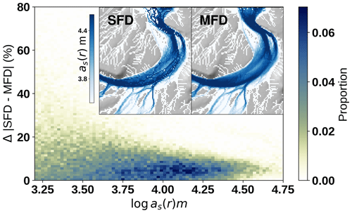
Figure 11 Differences in final results for a single flow solver and multiple flow solvers. The multiple-flow-direction solution is cleaner and has fewer artefacts. The magnitude of the differences is a function of the frequency at which the D8 single-flow-direction flow passes through a cell (proxied here by multiple flow directions, a_s(r)). While single-flow-direction solvers are faster and simpler, their accuracy will be a function of diverging flow patterns. Smaller Δt can reduce the differences.

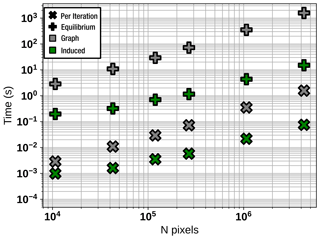
Figure 12 Time benchmark comparing the computational efficiency of GraphFlood and its induced graph variant for the Green River DEM resampled at various resolutions. The global convergence time represents the timing for converging the model for the fluvial and colluvial domains, while the time per iteration is an important metric when considering GraphFlood for LEMs.

Finally, the performances of GraphFlood are tightly linked to the numerical framework used for its implementation. The simplicity and versatility of GraphFlood make it straightforward to re-implement in different frameworks as long as they offer basic graph data structure and local minima handling. Computing the directed acyclic graph and the related algorithms for each iteration accounts for a big part of the computational time. Therefore, the implementations of these algorithms strongly impact the overall performances. For example, the exact same simulation takes approximately 250 or 800 ms in the Python/C++ implementation or using MATLAB©/TopoToolBox (Schwanghart and Scherler, 2014), respectively. The time-consuming algorithms are the topological ordering (e.g. Anand et al., 2020; Braun and Willett, 2013; Carretier et al., 2016), the local minima resolver (e.g. Cordonnier et al., 2019; Barnes et al., 2014; Gailleton et al., 2024), and the receiver and donor computations as they need updates at each iteration.

A detailed time benchmark comparison with other methods can also quickly be misleading because of the divergence of scopes: GraphFlood focuses on steady flow, which is conceptually too different to compare to transient solvers (e.g. Bates et al., 2010; Brunner, 2016). River.lab (Davy et al., 2017, formerly Floodos) also targets the stationary solution. Bernard (2022) demonstrated that the method could reach the same orders of magnitude for the time required to get a convergent solution in the main rivers in specific cases where the influx of precipitons is optimized to enter only the main channel via discrete inlets from tributary junctions. However, the efficiency of this method decreases when simulating other parts of the landscape, such as hillslopes, due to the low frequency of precipitation passage on non-convergent areas.

Nevertheless it is worth noting that the algorithm is scalable: the Green River site converges in about 20 s for the main rivers, with less than 200 ms per iteration. We also tested GraphFlood on an 83-million-pixel DEM on a laptop with 32 GB of memory, and the model converged for the main rivers in about 20 h with 100 s per iteration.

6.2 Potential optimizations

An obvious optimization consists of developing a parallel version of GraphFlood. In this paper, we made the choice to remain on a single-threaded CPU (i) for simplicity, (ii) for flexibility, and (iii) to favour the possibility of running concurrent models to explore parameter space. The transient mode can be parallelized, even on a GPU, as each node is independent of the others at a time t, similar to Apel et al. (2022). Stationary GraphFlood, on the other hand, has a strong non-local component in the calculation of Q_in and would require significant modification to be partially parallelized using, for example, Barnes et al. (2021) .

Another optimization consists of improving our management of time stepping. CFL conditions only theoretically apply to our calculation of Q_out but not to the propagation of Q_in in stationary mode. An alternative finite-difference formulation like Runge–Kutta or an implicit formulation could allow for larger time steps. However, these methods would only increase the efficiency of a single iteration but would still suffer from the highly iterative nature of the algorithm to reach an equilibrated hydraulic surface.

Finally, we can significantly reduce the computation time of studies interested in the fluvial domain only. As suggested in Bernard (2022) and illustrated in Fig. 4, GraphFlood converges significantly faster in areas with higher Q. The fluvial domain only represents a minor subset of the total number of nodes in a landscape, and theoretically, focusing only on these nodes could significantly speed up the process. Induced sub-graph methods offer solutions to apply algorithms in a subset of a directed acyclic graph without the need to process its entirety. In the case of rivers, it requires the identification of all the nodes of interest, i.e. downstream of a given discharge or drainage area threshold. Taking full advantage of this optimization is challenging as it requires the dynamic identification of the nodes of interest without processing the whole graph.

We developed an induced sub-graph method to take advantage of that optimization. The principle remains the same as in Sect. 3.1, except that graph-related operations are computed on a node-to-node basis (e.g. computing the directed acyclic graph donors and receivers, handling of local minima, topological ordering). A pre-computing step determines input points based on drainage area thresholds or arbitrary input points (Tarboton, 1997). These points are pushed in a priority queue that sorts active nodes per decreasing elevation (opposite to Barnes et al., 2014), ensuring that the most upstream node of interest that has not been processed yet is always next in queue. The nodes are popped and processed from the priority queue sequentially. Once Q_in and Q_out are computed according to Sect. 3.1, we push in the priority queue the receivers of the active node. The process is repeated until the queue is empty. Note that if a node has no receiver and is not a model edge, we gradually fill the local depression until an outlet is found, in a way similar to Davy et al. (2017) or Gailleton et al. (2024).

This version of the algorithm reproduces the results from the original one, except that there are minor artefacts near the input points. One iteration takes 250 ms with GraphFlood and 15 ms with the induced graph method. For a discharge threshold of 36 000 m² and a precipitation rate of 50 mm yr⁻¹, the models converge for the main rivers in about 50 s for GraphFlood vs. 3 s for the induced graph method, demonstrating strong potential for studies focusing on the fluvial domain. The complexity of the algorithm is tied to the priority queue and is therefore 𝒪(nlog n), with n being the number of nodes in each traversal, meaning computation time increases nonlinearly as the drainage area threshold decreases. Figure 12 provides an extensive time benchmark comparing the efficiency of both methods in a global and per-iteration perspective.

6.3 Potential for hydromorphometry and landscape evolution models

Bernard et al. (2022) demonstrated the potential of informing common scaling laws used in tectonic geomorphology (e.g. Kirby and Whipple, 2012) with hydrodynamics. GraphFlood represents a step toward making the inclusion of hydrology more systematic in geomorphological analysis. For example, s−a_s(r) plots, as illustrated by both Bernard et al. (2022) and Fig. 9, isolate more signals than classic S–A as per originally designed by Morisawa (1962) and Flint (1974). a_s(r) is not strictly a function of the downstream distance like A and has the potential to express a wider range of landforms. Data points with high a_s(r) and/or high s are likely to represent areas of increased stream power beyond the common geometrical knickpoint (e.g. increased discharge due to local channel narrowing), as demonstrated in Fig. B1. Alternatively, low s and low a_s testify to abnormally flat areas (i.e. flat areas not visited by rivers), which if calculated from multiple runoff rates could unravel families of terraces. Commonly used metrics linked to S–A (e.g. concavity index, steepness index) are likely to express a wider range of signals when extracted from s–a_s(r). Both our test sites and the study of Bernard (2022) show similar global patterns in s–a_s(r) plots while displaying notably different values, regression coefficient and intercept, and absolute values.

Combined with effective width or the direct calculation of shear stress from h, hydromorphometrics can help identify and quantify a new family of responses to perturbations. Alongside geometrical knickpoints (e.g. Gailleton et al., 2019), areas of channel narrowing or widening or accelerated flow can be identified, unravelling wider ranges of landscape responses to perturbations. Systematic calculations of all these metrics for multiple ranges of runoff rates could help redefine and complete global scaling laws comparing discharge, drainage area, channel width, and hydraulic slopes.

GraphFlood's ability to extract metrics for various precipitation rates also opens possibilities for indirect metrics. For instance, Clubb et al. (2022) and Clubb et al. (2023) highlighted the importance of valley width in understanding landscape evolution. By using extremely high precipitation rates with GraphFlood, it becomes possible to flood the valley and systematically determine its width. Another potential application could involve gradually increasing precipitation rates to progressively flood a fluvial system from its bed to its floodplain, revealing multiple families of terraces.

GraphFlood allows the fast approximation of hydrodynamics and therefore shear stress. Coupling GraphFlood with physics-based morphodynamics (e.g. Davy and Lague, 2009; Minor et al., 2022) would allow the upscaling of short-term fluvial dynamics to a longer timescale and larger spatial scales.

7 Conclusion

This study introduces GraphFlood, an efficient algorithm for solving 2D hydrodynamics based on 2D shallow-water equations specifically tailored for large DEMs. By employing Manning's equation within a graph theory framework, GraphFlood iteratively computes a stationary flow depth and discharge equilibrated to prescribed runoff rates. Leveraging graph theory algorithms ensures numerical efficiency, enabling GraphFlood to compute solutions for rivers in just seconds for a million-pixel DEM. Validation against analytical solutions and established models demonstrates the accuracy of GraphFlood. The simplicity, efficiency, and versatility of GraphFlood position it as a promising engine for incorporating 2D hydrodynamics into large-scale topographic analysis and landscape evolution models. Future work could utilize GraphFlood to investigate river inundation patterns, systematically extract river width as a function of water discharge, or focus on classifying landscapes to better relate landscape shape to geomorphological processes.

Appendix A: Notations

Table A1 Nomenclature for scientific notations.

Appendix B: Outliers in s–a_s(r)

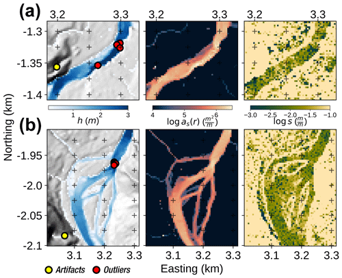
Figure B1 Zoom-in on outliers for the Hanalei test site, isolated using data from Fig. 9. From left to right, the maps show the flow depth with the localization of the outliers, the specific area, and the hydraulic slope. Panel (a) displays outliers concentrating flow on a narrowing section of the river or on its bends. Panel (b) shows the case of converging branches. In both cases, outliers are accompanied by a slight increase in s.