Influence of cohesive clay on wave–current ripple dynamics captured in a 3D phase diagram

Wave–current ripples that develop on seabeds of mixed non-cohesive sand and cohesive clay are commonplace in coastal and estuarine environments. While laboratory research on ripples forming in these types of mixed-bed environments is relatively limited, it has identified deep cleaning, the removal of clay below the ripple troughs, as an important factor controlling ripple development. New large-scale flume experiments seek to address this sparsity in data by considering two wave–current conditions with initial clay content, C₀, ranging from 0 % to 18.3 %. The experiments record ripple development and pre- and post-experiment bed clay contents to quantify clay winnowing. The present experiments are combined with previous wave-only, wave–current, and current-only experiments to produce a consistent picture of larger and smaller flatter ripples over a range of wave–current conditions and C₀. Specifically, the results reveal a sudden decrease in the ripple steepness for C₀ > 10.6 %, likely associated with a decrease in hydraulic conductivity of 3 orders of magnitude. Accompanying the sudden change in steepness is a gradual linear decrease in wavelength with C₀ for C₀ > 7.4 %. Ultimately, for the highest values of C₀, the bed remains flat, but clay winnowing still takes place, albeit at a rate 2 orders of magnitude lower than for rippled beds. For a given flow, the initiation time, when ripples first appear on a flat bed, increases with increasing C₀. This, together with the fact that the bed remains flat for the highest values of C₀, demonstrates that the threshold of motion increases with C₀. The inferred threshold enhancement, and the occurrence of large and small ripples, is used to construct a new three-dimensional phase diagram of bed characteristics involving the wave and current Shields parameters and C₀, which has important implications for morphodynamic modelling.

1 Introduction

In coastal and estuarine environments, the superposition of waves and currents, termed combined wave–current flows, is a common occurrence. In these environments, which include continental shelves, the shoreface, and tidal flats, combined wave–current flows frequently form ripples on the seabed (e.g. Osborne and Greenwood, 1993; Li and Amos, 1999; Héquette et al., 2008; Gao, 2019). Ripple dynamics play a crucial role in sediment transport, which in turn affects the prediction of large-scale coastal morphodynamic numerical models (Brakenhoff et al., 2020), the underwater scour around civil engineering structures (Sumer et al., 2001), and the transport of nutrients and contaminants (Vercruysse et al., 2017). Moreover, combined-flow ripples have been found in the geological record, thus providing key information for reconstructing palaeoenvironments (e.g. Myrow et al., 2006; Beard et al., 2017). It is therefore crucial to examine how combined-flow hydrodynamics control ripple dimensions and vice versa, particularly in muddy coastal and estuarine environments that are widespread in nature (Healy et al., 2002) and characterized by sediment consisting of a mixture of cohesive clay and non-cohesive sand. A full understanding of this process will ultimately prove significant for coastal and estuarine management and ecological balance maintenance, especially as such areas may face more extreme weather events in the context of climate change and sea level rise (e.g. Mousavi et al., 2011; Vitousek et al., 2017).

To date, however, there has been a scarcity of relevant literature on this topic. Wu et al. (2022) were the first to consider ripple dynamics in sand–clay mixtures under combined flows. Their study showed that small flat ripples formed for initial clay contents, C₀, greater than 10.6 % under hydrodynamic conditions that formed large equilibrium ripples in clean sand. Moreover, Wu et al. (2022) demonstrated that clay winnowing efficiency plays a significant role in the development towards clean-sand-like ripples on mixed sand–clay beds. They also highlighted the process of deep cleaning of clay below ripple troughs for C₀≤ 10.6 %, whereas Wu et al. (2018) revealed a more modest deep accumulation of clay beneath rippled beds under wave-only conditions for C₀≤ 7.4 %. This suggests a dynamic balance between loss and accumulation of clay during ripple development. However, the key factors governing this dynamic balance, and the resulting ripple size, remain unclear, primarily due to the limited number of flow conditions considered thus far. This knowledge deficiency in mixed sand–clay experiments is reflected in the existing ripple predictors, i.e. bedform phase diagrams and empirical formulae, that are based exclusively on clean-sand experiments.

Phase diagrams group similar bedform types and cross-sectional geometries for known hydrodynamic conditions and sediment properties (e.g. Van den Berg and Van Gelder, 1993). In the last 30 years, a substantial number of experimental studies have made progress in compiling combined-flow ripple phase diagrams (Arnott and Southard, 1990; Kleinhans, 2005; Dumas et al., 2005; Cummings et al., 2009; Perillo et al., 2014). Using a range of combined-flow conditions in an experimental flume, Perillo et al. (2014) expanded the bedform phase diagrams of Arnott and Southard (1990) and Dumas et al. (2005) by subdividing bedform types based on planform geometry. The phase diagram of Baas et al. (2021), based on field observations of bedforms on an intertidal flat in the Dee Estuary, UK, captured bedform types generated under a wider range of flow conditions, including those generated under waves and currents at angles to one another. Compared to wave-only and current-only ripple predictors, relatively few predictors are available for combined-flow ripples. Tanaka and Dang (1996) modified a widely used predictor for wave ripples developed by Wiberg and Harris (1994) by considering the influence of grain size and the relative strength of the wave and current velocities on the ripple size. Khelifa and Ouellet (2000) developed a new formulation to predict ripple dimensions by introducing an effective combined-flow mobility parameter.

The experiments of Wu et al. (2022) were conducted under a single wave-dominated combined-flow condition, but further study considering wider hydrodynamic conditions is required for a more comprehensive understanding of the interaction between ripple development and winnowing-induced clay loss from beds. These insights are critical for the development of morphodynamic models applicable in muddy estuaries and the coastal zone. Therefore, the present study extends the experiments of Wu et al. (2022) and describes a systematically collected set of data from large-scale flume experiments on ripple development. This study also draws in available sand–clay experiments under current-only and wave-only conditions (Baas et al., 2013; Wu et al., 2018). The three specific objectives of this study were (1) to compare ripple development and occurrence on beds with similar initial clay contents under different hydrodynamic conditions; (2) to compare clay winnowing efficiency during ripple development, under different flow conditions; and (3) to propose a new phase diagram for bedforms generated in sand–clay substrates to systematize the experiments, using the knowledge gained from objectives 1 and 2.

2 Materials and methods

2.1 Experiment setup

The experiments were undertaken in a recirculating flume tank in the Total Environment Simulator at the University of Hull. Three equal-size channels, 11 m long and 1.6 m wide, were separated by brick walls, 0.2 m high, in the tank (Fig. 1). Combined-flow conditions were maintained during the experiments and flow velocities in each channel were measured by a 25 Hz Vectrino profiler throughout the entire duration of the experiments. Freshwater was used in all experiments, and the water depth, h, was set to 0.4 m. A 2 MHz ultrasonic ranging sensor (URS), containing 32 probes, monitored the ripple evolution and migration in the test section (Fig. 1). Further details of the instrument setup are available in Wu et al. (2022).

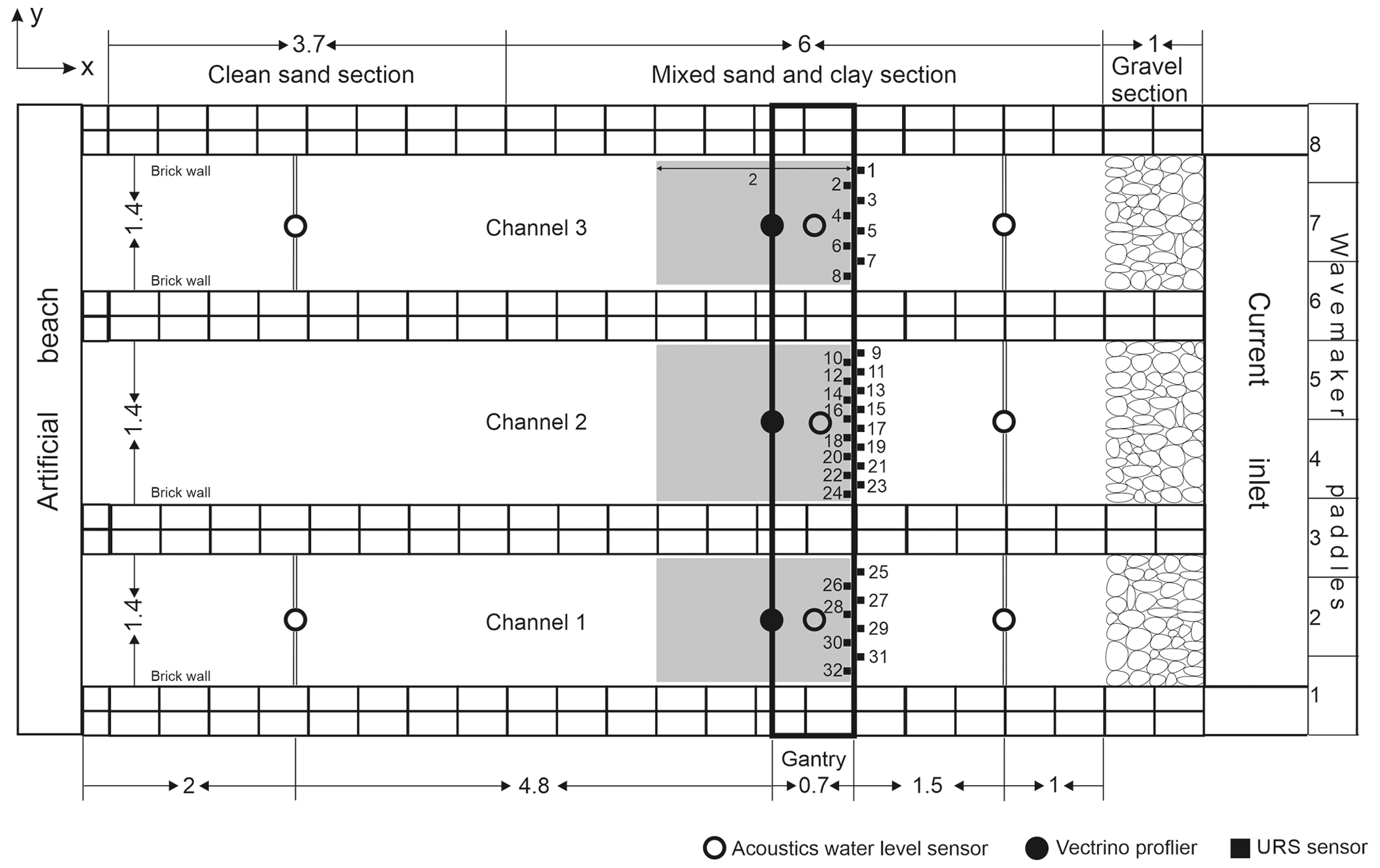
Figure 1 Plan view of the experimental setup. The grey area was scanned by an ultrasonic ranging sensor (URS) with numbered probes (black squares). White and black circles denote acoustic water level sensors and Vectrino profilers respectively. Dimensions are in metres.

2.2 Experimental procedure and wave–current settings

To complement the wave-dominated flow condition of Wu et al. (2022), with depth-average current, U_c≈ 0.16 m s⁻¹, and wave velocity amplitude, U_w≈ 0.32 m s⁻¹ (Appendix Table A1), the present experiments comprised two additional flow conditions of increased relative current strength, with U_c≈ 0.3 m s⁻¹ and U_w≈ 0.27 and 0.13 m s⁻¹, with wave heights, H, of 0.05 and 0.1 m, and wave period, T, of 2 s (Table 1). The wave–current flow conditions (WC1, in Table A1 from Wu et al., 2022; WC2 and WC3, in Table 1) are numbered according to increasing relative current strength, from the weakest, WC1, to the strongest, WC3. The experiments involved different initial mass concentrations of clay, C₀, in each of the three channels, with the same flow conditions for each channel. The bed was composed of a well-sorted sand with a median diameter, D₅₀, of 0.45 mm and cohesive kaolinite clay with D₅₀= 0.0089 mm. The sand, clay, water depth, and wave period in the present experiments were the same as in Wu et al. (2022). The order of the experiments was from high to low clay content, by taking advantage of the natural winnowing of the bed during the experiments. Run 1, the sand-only control, and Run 2, with C₀ of 9.9 %, 13.1 %, and 18.3 % by dry weight in channels 1 to 3, were under WC3 flow conditions (Table 1). The beds in Run 2 remained essentially flat after 650 min. In Run 3, the wave height was doubled (WC2) and the duration was increased to 1850 min. In Run 4, three beds were prepared with relatively low clay contents, C₀≤ 6.4 %, and the same WC3 conditions as in Runs 1 and 2 were imposed.

Table 1 Experimental parameters.

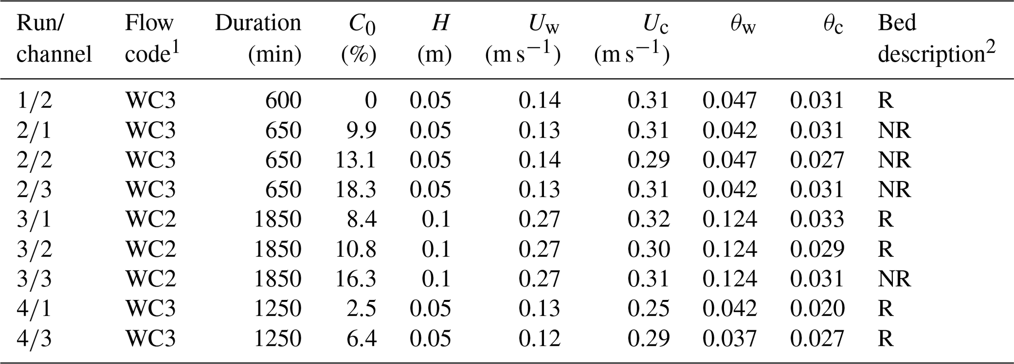
¹The flow code represents the relative current strength, where WC1 (Wu et al., 2022, Table A1) is the weakest and WC3 is the strongest. For WC1 conditions (Table A1), corresponding to 0 $\le C_{\mathrm{0}}\le$ 12.6, 0.31 $\le U_{\mathrm{w}}\le$ 0.33 m s⁻¹, 0.15 $\le U_{\mathrm{c}}\le$ 0.2 m s⁻¹, 0.15 ≤ θ_w≤ 0.16, and 0.007 $\le {\mathit{\theta }}_{\mathrm{c}}\le$ 0.13, ripples always developed. ² R – ripples formed; NR – no ripples formed.

To ensure homogeneity in the mixed section of each channel (Fig. 1), the clay was mixed into the sand using a handheld plasterer's mixer and the sediment beds were flattened using a wooden leveller between runs. A terrestrial 3D laser scanner (FARO Focus3D X330) was used to scan the sediment bed in each channel before and after the run, after the water had been drained. Furthermore, the flow was temporarily stopped during the runs at pre-set times to make URS bed scans and collect sediment cores from the bed using syringes with a diameter of 20 mm and a maximum length of 90 mm. These short pauses in the experiments resulted in negligible bed deposition of suspended clay particles due to their slow settling velocity. Details of the protocols for URS bed scanning and sediment core collection are available in Wu et al. (2022). Channel 2 of Run 4 was excluded from the analysis, because core samples collected from the flat bed showed that the sediment in this channel was not sufficiently well mixed.

Wu et al. (2022) justified their choice of flow conditions by demonstrating that they were largely consistent with the observations of the intertidal field site in the macrotidal Dee Estuary (UK) of Baas et al. (2021), where D₅₀= 0.227 mm, 0 < h≤ 3.5 m, 0 < U_c≤ 0.6 m s⁻¹, 0 < U_w≤ 0.45 m s⁻¹, and 0 < C₀≤ 14 %. Baas et al. (2021) produced a phase diagram based on the equivalent wave-only and current-only skin friction, τ_w and τ_c, using the shear stress calculation of Malarkey and Davies (2012) with the strong non-linear option. Here in Fig. 2, the phase diagram of Baas et al. (2021) has been non-dimensionalized to the equivalent wave-only and current-only Shields parameters, θ_w and θ_c, given by $\mathit{\tau }/({\mathit{\rho }}_{\mathrm{s}}-\mathit{\rho })g{D}_{\mathrm{50}}$, where ρ_s is the sediment density (= 2650 kg m⁻³), ρ is the water density (= 1000 kg m⁻³ for freshwater, 1027 kg m⁻³ for seawater), and g is the acceleration due to gravity (= 9.81 m s⁻²). This allows the present experiments (Table 1, WC2 and WC3) and previous wave–current experiments (WC1, Table A1), together with the current-only and wave-only experiments of Baas et al. (2013) and Wu et al. (2018) (Tables A2 and A3), to be compared to one another. In Fig. 2, the critical Shields parameter for the clean-sand threshold of motion, θ₀, is determined with the formula of Soulsby (1997), θ₀= $\mathrm{0.3}/(\mathrm{1}+\mathrm{1.2}{D}_{*})+\mathrm{0.055}[\mathrm{1}-\exp (-\mathrm{0.02}{D}_{*}\left)\right]$, where $D_{*}=D_{\mathrm{50}}\left[\right({\mathit{\rho }}_{\mathrm{s}}-\mathit{\rho })g{\mathit{\nu }}^{\mathrm{2}}/\mathit{\rho }{]}^{\mathrm{1}/\mathrm{3}}$ and ν is the kinematic viscosity of water. It should be noted that the threshold of motion is different for each grain size: θ₀= 0.032 for WC1–WC3, where D₅₀= 0.45 mm; θ₀= 0.032 for Wu et al. (2018), where D₅₀= 0.496 mm; θ₀= 0.061 for Baas et al. (2013), where D₅₀= 0.143 mm; and θ₀= 0.05 for Baas et al. (2021), where D₅₀= 0.227 mm. In Fig. 2 the threshold of motion appears as a straight line given by ${\mathit{\theta }}_{\mathrm{w}}+{\mathit{\theta }}_{\mathrm{c}}={\mathit{\theta }}_{\mathrm{0}}$ because, unlike in the field study of Baas et al. (2021), all experimental flows were co-linear. Whilst θ₀ is clearly affected by grain size, it is assumed that the other boundaries in the phase diagram are not.

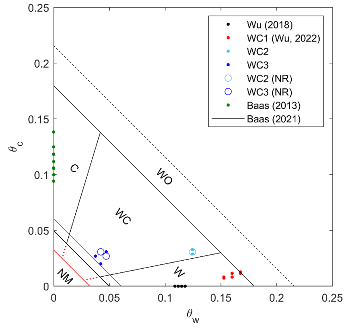
Figure 2 Non-dimensional, θ_w–θ_c phase diagram after Baas et al. (2021), showing all wave-only (Wu et al., 2018), wave–current, WC1 (Wu et al., 2022), WC2, WC3, and current-only (Baas et al., 2013) conditions. Open circles show cases where no ripples (NR) were present, and the various regions are marked C – current-dominant, WC – wave–current, W – wave-dominant, NM – no motion, and WO – washout. The additional threshold of motion lines, θ₀, are coloured red for WC1–WC3 and Wu et al. (2018) and green for Baas et al. (2013).

The phase diagram (Fig. 2) identifies the flow conditions of Wu et al. (2018) and WC1 as wave-dominated (W), θ_c < 0.2θ_w, those of Baas et al. (2013) as current-dominated (C), θ_c > 3.3θ_w, and those of the present experiments (WC2 and WC3) as wave–current (WC), 0.2θ_w < θ_c < 3.3θ_w. Whilst not all experiments produced ripples (open circles and NR in Table 1), all the data were between the washout limit ${\mathit{\theta }}_{\mathrm{w}}+{\mathit{\theta }}_{\mathrm{c}}=$ 0.18 and the clean-sand threshold of motion, ${\mathit{\theta }}_{\mathrm{w}}+{\mathit{\theta }}_{\mathrm{c}}={\mathit{\theta }}_{\mathrm{0}}$. It is anticipated that ultimately above washout there are flat featureless upper stage plane beds (for waves and currents at angles this may be complicated by the occurrence of lunate ripples, Baas et al., 2021). The reason that not all conditions produce ripples is related to higher clay contents enhancing the threshold shear stress. This is a shortcoming of the phase diagram of Baas et al. (2021) and is the justification for the new phase diagram proposed in this paper.

2.3 Data processing

Raw bed elevation profiles recorded from each URS scan, consisting of 16 profiles for channel 2 and 8 profiles for channels 1 and 3, were processed after de-spiking and smoothing. A MATLAB “peaks and troughs” tool was used to identify individual ripple heights, η, and wavelengths, λ, followed by calculation of the mean across-channel values of λ_t and η_t at a bed scanning time of t to construct the development curves of ripple height and wavelength and hence determine equilibrium bedform dimensions. Following Wu et al. (2022), the equilibrium ripple height, η_e, and wavelength, λ_e, and equilibrium time for ripple height, T_η, and wavelength, T_λ, were calculated using the procedure of Baas et al. (2013), which includes a delay time for the first appearance of ripples, t_i, and an initial wavelength, λ_i:

$$\begin{array}{}\text{(1)}& {\displaystyle \frac{{\mathit{\eta }}_t}{{\mathit{\eta }}_{\mathrm{e}}}}=\mathrm{1}-{\mathrm{0.1}}^{\frac{t-t_i}{T_{\mathit{\eta }}-t_i}},\text{(2)}& {\displaystyle \frac{{\mathit{\lambda }}_t-{\mathit{\lambda }}_i}{{\mathit{\lambda }}_{\mathrm{e}}-{\mathit{\lambda }}_i}}=\mathrm{1}-{\mathrm{0.1}}^{\frac{t-t_i}{T_{\mathit{\lambda }}-t_i}},\end{array}$$

The ripples were also characterized by their steepness, RS, and ripple symmetry index, RSI, given by

$$\begin{array}{}\text{(3)}& {\displaystyle }\mathrm{RS}={\mathit{\eta }}_{\mathrm{e}}/{\mathit{\lambda }}_{\mathrm{e}},\text{(4)}& {\displaystyle }\mathrm{RSI}={\mathit{\lambda }}_{\mathrm{s}}/{\mathit{\lambda }}_{\mathrm{l}},\end{array}$$

where λ_s and λ_l are the length of the stoss and lee side of the ripple (RSI < 1.3 for symmetric and 1.3 < RSI < 1.5 for quasi-asymmetric ripples, Perillo et al., 2014) (Table 2).

Table 2 Bedform characteristics.

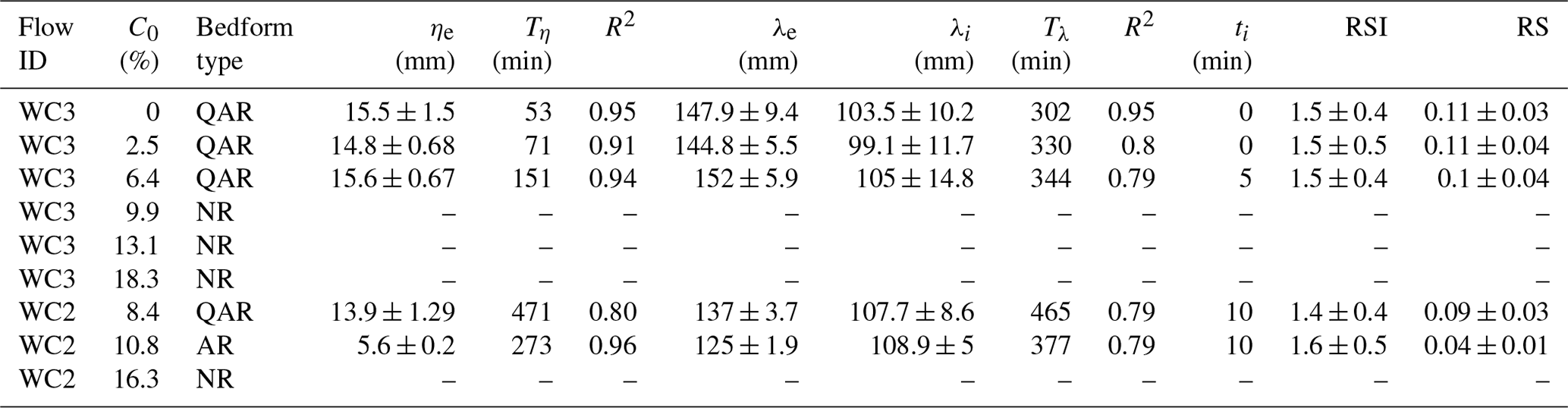
QAR: quasi-asymmetric ripple. AR: asymmetric ripple. NR: no ripples. R²: squared correlation coefficient of the best fit curve. The values given after ± are 1 standard deviation.

Sediment cores from the initial flat bed and the ripple crests and troughs were sliced into 10 mm intervals for grain-size analysis using a Malvern Mastersizer 2000. In the crest cores, the region corresponding to the active layer (ripple crest down to trough) was sliced into 5 mm intervals for better resolution of the clay content within the ripples. The measured clay content, C, in the sediment cores was further processed to acquire the total amount of clay removed from the bed, I, by integrating the clay deficit, defined as $C_{\mathrm{def}}=C_{\mathrm{0}}-C$, from the lowest reference level, $z=-\mathrm{100}$ mm up to the crest level, z= 0 mm. These quantities allow the equivalent clean-sand depth, d_c, to be given by

$$\begin{array}{}\text{(5)}& d_{\mathrm{c}}=I/C_{\mathrm{0}},\end{array}$$

which is the amount of clean sand available in the uppermost layers for ripple growth. Finally, the sediment concentration profiles were characterized by a Gaussian-type function. Full details of all data processing are available in Wu et al. (2022).

3 Results

3.1 Ripple development

Figure 3 shows the development of ripple height and wavelength for different C₀ values in the present experiments (WC2 and WC3). For C₀= 0 % (WC3), clean-sand ripples appeared immediately after the start of the experiment (t_i= 0), developed rapidly and reached an equilibrium height and wavelength of η_e= 15.5 mm and λ_e= 147.9 mm (Fig. 3a and b; Table 2). As shown in Fig. 4a, the clean-sand ripples were two-dimensional in plan view, with straight continuous crest lines. In cross section, these ripples were quasi-asymmetric, with a ripple symmetry index (RSI) of 1.4 and a ripple steepness (RS) of 0.11 (Table 2).

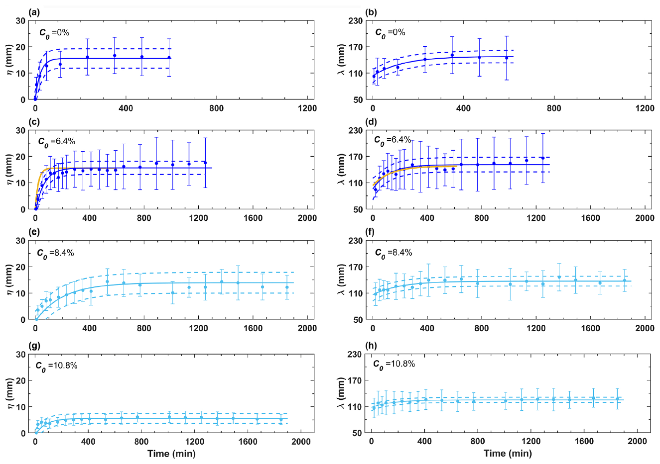
Figure 3 Development of ripple height and wavelength for WC3 (dark blue dots in a–d) and WC2 (light blue dots in e–f) for different values of C₀. The error bars denote 1 standard deviation from the mean dimension. Continuous dark and light blue lines are based on fitting to Eqs. (1) and (2), and dashed dark and light blue lines are their corresponding 95 % confidence intervals. The yellow lines in (c) and (d) are the best-fit curves for clean sand from (a) and (b).

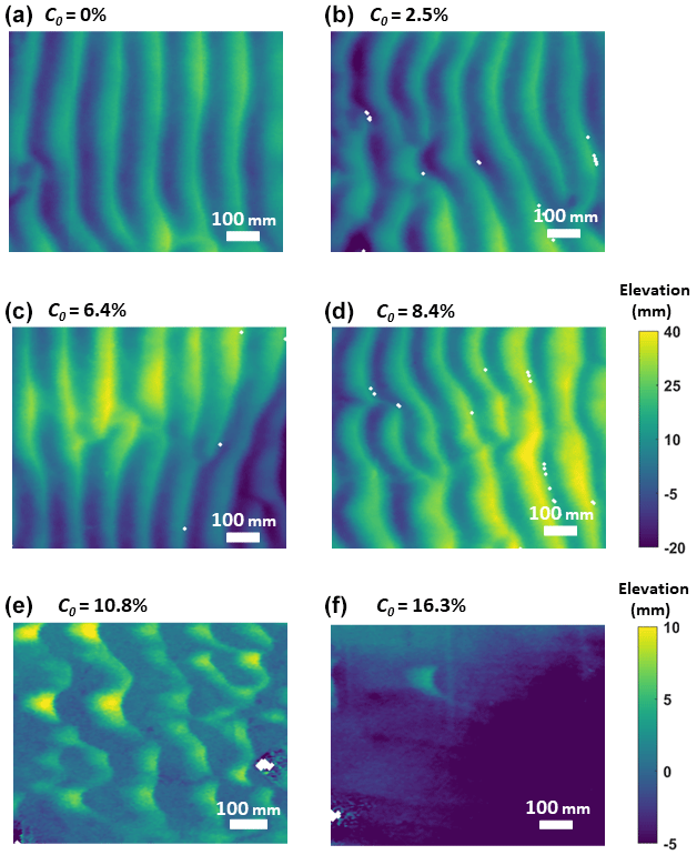
Figure 4 Plan view of ripple morphology in the test section acquired by the 3D FARO scanner at the end of the experiment. (a–c) rippled beds formed under WC3 conditions; (d–f) bed states under WC2 conditions. C₀ is the initial clay content, and the flow direction is from left to right. Note the elevation scale for (d) also applies to (a)–(c), and elevation scale for (f) also applies to (e).

For C₀= 2.5 % and 6.4 % (WC3), the ripples developed to similar equilibrium dimensions as their clean-sand counterparts, η_e= 15.6 mm and λ_e= 152.5 mm for C₀= 6.4 % (Fig. 3c and d), and the bed was again covered in two-dimensional, quasi-asymmetric ripples (Fig. 4b and c).

The three WC3 cases with C₀≥ 9.9 % remained flat over the entire 10 h duration (Table 2), implying there was no sand movement in these cases. Despite flat-bed conditions persisting, winnowing during the experiment caused the bed clay content to decrease, as will be seen in the next section, such that the initial clay contents were C₀= 8.4 %, 10.8 %, and 16.3 % for the three channels in the subsequent run under WC2 conditions, where U_w was doubled to 0.27 m s⁻¹. For C₀= 8.4 % (WC2), small ripples appeared at t= 10 min. Thereafter, ripple dimensions developed gradually over a period of around 7 h, stabilizing to an equilibrium height and wavelength of 13.9 and 137 mm (Fig. 3e and f). The equilibrium ripples retained similar geometries to those developed under WC2 conditions, characterized by two-dimensional plan forms with quasi-asymmetric cross sections (Table 2; Fig. 4d).

At C₀= 10.8 % (WC2), ripples again appeared at t= 10 min but only grew to equilibrium dimensions of η_e= 5.6 mm and λ_e= 125 mm (Fig. 3g and h, Table 2). These small ripples were three-dimensional with discontinuous, sinuous crest lines in plan view. In cross section, these ripples were asymmetric and flatter, with RSI = 1.6 and RS = 0.04 (Fig. 4e, Table 2). The general trends in equilibrium time for ripple height, T_η, and wavelength, T_λ, with C₀ were similar to those found by Wu et al. (2022). For the C₀= 16.3 % (WC2) case, the bed remained flat (Fig. 4f); there was no sand movement.

3.2 Comparison of pre- and post-experiment vertical bed clay content

Figure 5 shows the pre- and post-experiment vertical clay content in the bed, based on grain-size analysis of the sediment cores. In each case, the vertical solid and dashed grey lines show the value of C₀ ± 1 standard deviation. Figure 5a–d show the pre-experiment clay contents and Fig. 5e–h show the post-experiment clay contents for WC3. The three WC3 flat-bed cases (Fig. 5f–h) were used as the pre-experiment cores for WC2, with post-experiment cores shown in Fig. 5i–k. For WC3, C₀= 6.4 %, the sediment cores show a 100 % clay loss in the active layer (ripple crest down to the ripple trough level) and an additional layer of substantial clay loss with a thickness of ca. 80 mm below the active layer (Fig. 5e). The equivalent clean-sand depth (horizontal dashed black line), $d_{\mathrm{c}}=I/C_{\mathrm{0}}$, was 57 mm, more than 2 times the ripple height (25 mm). For WC2, C₀= 8.4 % (Fig. 5i), a small amount of clay, 2.9 %, remained at the base of the active layer. In contrast to the C₀= 6.4 % case, d_c= 13.1 mm is smaller than the ripple height (17.5 mm). For C₀= 10.8 % (Fig. 5j), there were much smaller ripples (Fig. 3g and h, and Table 2), which contained a higher clay content of 8 % at the base of the active layer. Here, d_c= 10.1 mm, compared to the ripple height of 5.6 mm.

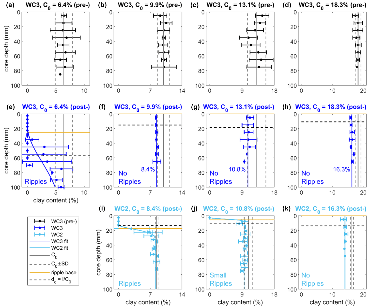
Figure 5 Pre-and post-experiment vertical profiles of clay content in cores collected from beds in the mixed sand–clay section. In each case, the pre- and post-experiment profiles are directly above one another: for WC3 conditions (pre-experiment a–d and post-experiment e–h) and for WC2 conditions (pre-experiment f–h and post-experiment i–k). Note the three WC3 flat-bed cases (f–h) were used as the pre-experiment cores for WC2 (i–k). The solid dark/light blue lines are the fits to WC3/WC2 post-experiment clay contents at each depth. The vertical solid and dashed grey lines represent mean initial clay content, C₀, and 1 standard deviation from the mean for comparison. The horizontal error bars denote 1 standard deviation of the mean clay content at that depth. For post-experiment cores, the yellow lines represent the ripple base and the dashed horizontal black lines represent the equivalent clean-sand depth.

No ripples formed for C₀≥ 9.9 % under WC3 conditions and C₀= 16.3 % under WC2 conditions (Table 2). Nevertheless, the post-experiment sediment cores clearly demonstrate clay loss at all measured depths (Fig. 5f–h and k). Specifically, there was an approximate 10 % reduction in clay content on beds with C₀= 16.3 % and 18.3 %, whereas there was a higher percentage of clay loss from the lower C₀ beds: 15 % for C₀= 9.9 % and 18 % for C₀= 13.1 %. This difference is reflected in the d_c values: 15 and 19 mm for C₀= 9.9 % and 13.1 % compared to 14 and 11 mm for C₀= 16.3 % and 18.3 %.

4 Discussion

4.1 The effect of clay and hydrodynamic conditions on ripple dimensions and geometries

The experiments of Wu et al. (2022), under WC1 flow conditions, revealed two distinct types of equilibrium ripples with a threshold C₀ value of 10.6 %. For C₀≤ 10.6 %, large 2D ripples with similar dimensions and geometries to their clean-sand counterparts developed, whereas for C₀ > 10.6 % only small flat 3D ripples developed. In the present experiments under WC2 conditions, this discontinuity in equilibrium ripple size was also observed (Table 2), with small equilibrium ripples generated in the C₀= 10.8 % case, consistent with C₀ > 10.6 %. Additionally, the clay content at the base of the active layer was ca. 8 %, which is consistent with the threshold of Wu et al. (2022) that restricts the ripples from growing beyond their small, flat stage. Wu et al. (2022) argued that this latter 8 % threshold was more general than the C₀= 10.6 % threshold as it was also found to be the case at the base of the active layer for the C₀= 13 % threshold of Baas et al. (2013) for fine-sand current ripple sizes (Table A2).

Figure 6a, which includes WC1–WC3 and the wave-only cases of Wu et al. (2018), shows that the two ripple types correspond to two quite distinct constant steepness groupings, RS, which change at C₀= 10.6 %. For WC3 conditions, the C₀= 10.6 % small–large ripple threshold is hypothetical as the bed shear stresses for what would be small ripples are below the threshold of motion for C₀≥ 9.9 %, and hence no ripples form (RS = 0). The threshold of motion will be discussed in Sect. 4.3. Figure 6a demonstrates another feature of the larger wave-only and wave–current ripples which can also be seen in the data of Perillo et al. (2014). The steepness is directly related to the current shear stress: RS = 0.145 for Wu et al. (2018), where θ_c= 0; RS = 0.120 for WC1, where θ_c= 0.008–0.013; and RS = 0.103 for WC2 and WC3, where θ_c= 0.020-0.033 (Tables 1, A1, and A3, and Fig. 2). This is the background current shear stress limiting the growth of wave ripples with increasing effect, such that for the strongest current the steepness is only just above the threshold for boundary-layer separation and vortex ejection (RS > 0.1, Sleath, 1984). Compared to the large ripples, the steepness of the small ripples was 0.04, implying there was no boundary layer separation (Fig. 6a and Wu et al., 2022).

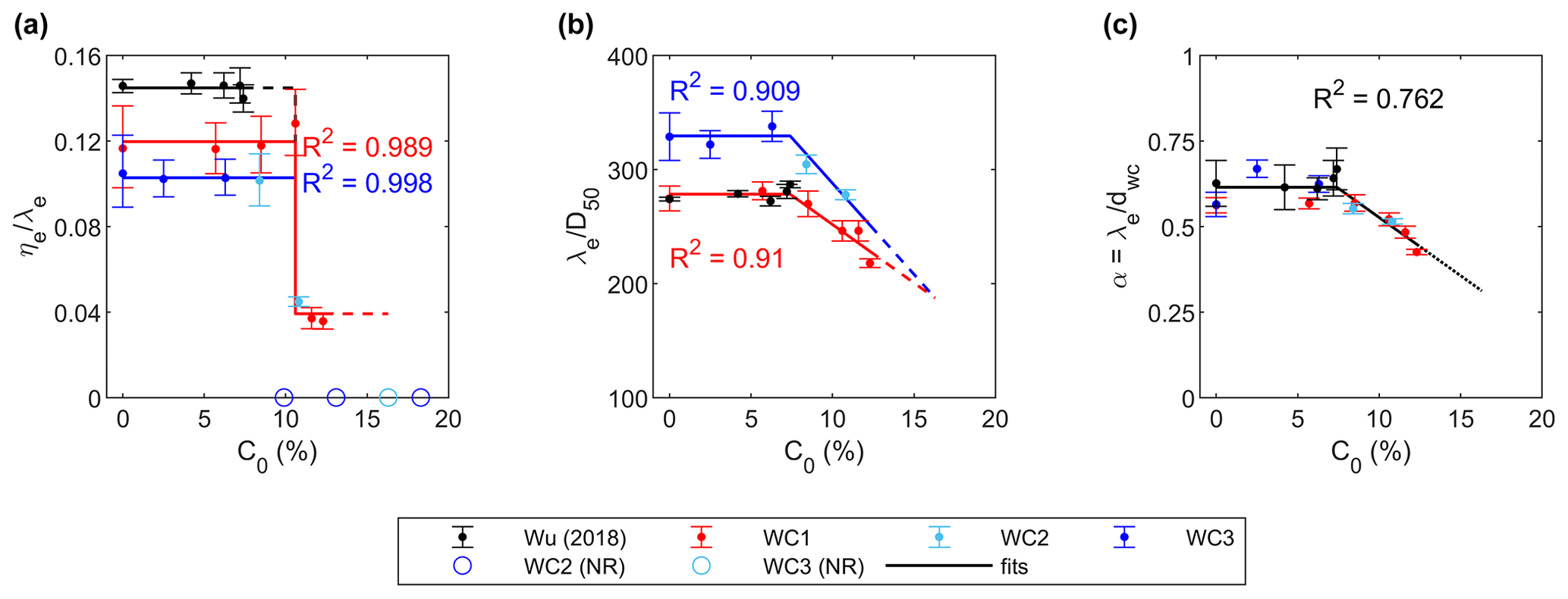
Figure 6 Equilibrium ripple steepness, RS $={\mathit{\eta }}_{\mathrm{e}}/{\mathit{\lambda }}_{\mathrm{e}}$, (a); non-dimensional ripple wavelength, ${\mathit{\lambda }}_{\mathrm{e}}/D_{\mathrm{50}}$, (b); and the α parameter, $\mathit{\alpha }={\mathit{\lambda }}_{\mathrm{e}}/d_{\mathrm{wc}}$, (c), as a function of initial bed clay content, C₀, for Wu et al. (2018) and WC1–WC3. Open circles show that no ripples (NR) were present and dots are based on measured values of η_e, λ_e, and α and their error bars. Solid lines correspond to least-squares fits to the data with R² values quoted.

Other than this reduction in steepness, current strength was found to have a modest influence on ripple geometry; for example, RSI ≈ 1.5 for the large ripples for WC2 and WC3 (Table 2) compared to RSI ≈ 1.4 for WC1 (Wu et al., 2022). However, previous flume experiments with an increasing current component have shown a more dramatic effect (Yokokawa, 1995; Dumas et al., 2005; Perillo et al., 2014). Perillo et al. (2014) found that ripples became more asymmetric, with RSI increasing from 1.4 to 1.7, as U_c increased from 0.1 to 0.3 m s⁻¹, with U_w= 0.25 m s⁻¹. The relatively coarse sediment used in WC1–WC3, D₅₀= 0.45 mm, may have resulted in a greater tendency towards 2D symmetric ripples, compared to the finer sediment of Perillo et al. (2014), D₅₀= 0.25 mm, forming more 3D asymmetric ripples (Cummings et al., 2009; Pedocchi and García, 2009).

Figure 6b shows that the non-dimensional equilibrium wavelength, ${\mathit{\lambda }}_{\mathrm{e}}/D_{\mathrm{50}}$, is approximately constant for C₀≤ 7.4 %. However, unlike the ripple steepness, there is a gradual linear reduction with C₀ for C₀ > 7.4 % (the upper limit of the experiments of Wu et al., 2018). Interestingly, this 7.4 % limit is very similar to the 8 % limit at the base of the active layer discussed above. Based on the trend lines fitted to the data in Fig. 6b, the clean-sand equivalent equilibrium ripple wavelengths fall into two distinct groups: a wave-dominant group, comprising the WC1 and Wu et al. (2018) cases, where ${\mathit{\lambda }}_{\mathrm{e}}/D_{\mathrm{50}}=$ 278, and a wave–current group, comprising the WC2 and WC3 cases, where ${\mathit{\lambda }}_{\mathrm{e}}/D_{\mathrm{50}}=$ 329 (18 % larger). All ripples with C₀≤ 10.6 % are clearly 2D and orbital in nature (Fig. 4a–d; Fig. 3a–d in Wu et al., 2022, 2018), including such characteristic features as bifurcations (Perron et al., 2018), implying that the wavelength is directly proportional to the wave orbital diameter. This together with the fact that skin friction stresses show that the flow can reverse (θ_w > θ_c), even for WC3 conditions, implies that the wavelength should be described by λ_e=αd_wc, where α is the constant of proportionality (= 0.62, according to Wiberg and Harris, 1994) and d_wc is the orbital diameter enhanced by the current. The orbital diameter scales the ripple spacing, as it represents the distance a neutrally buoyant particle can move in half a wave cycle (Clifton and Dingler, 1984). With the addition of a current, this particle can move further and Appendix B explains how d_wc is determined based on a sinusoidal wave. The value of d_wc is open to some interpretation, as the near-bed wave orbital diameter is combined with the depth-averaged current. Here, it has been chosen to reflect the difference in the clean-sand values of ${\mathit{\lambda }}_{\mathrm{e}}/D_{\mathrm{50}}$ between the two groups: $d_{\mathrm{wc}}/D_{\mathrm{50}}=$ 469 and 539, for the wave-dominant and wave–current groups respectively. The Wiberg and Harris (1994) definition confirms that these flows are both within the orbital ripple regime ($d_{\mathrm{wc}}/D_{\mathrm{50}}\le$ 1754).

With the wave–current orbital diameter, d_wc, now determined, it is possible to calculate the quantity α ($={\mathit{\lambda }}_{\mathrm{e}}/d_{\mathrm{wc}}$), which is shown in Fig. 6c. While there is scatter (R²= 0.762), all the data collapse onto a single curve with a similar behaviour to the wavelength (Fig. 6b):

$$\begin{array}{}\text{(6)}& \mathit{\alpha }=\left\{\begin{array}{ll}\mathrm{0.61},& C_{\mathrm{0}}\le C_{\mathrm{0}\mathrm{m}},\\ \mathrm{0.61}-\mathrm{3.36}(C_{\mathrm{0}}-C_{\mathrm{0}\mathrm{m}}),& C_{\mathrm{0}}>C_{\mathrm{0}\mathrm{m}},\end{array}\right.\end{array}$$

where C_0m= 7.4 %, such that α= 0.31 when C₀= 16.3 %. For C₀≤ 7.4 %, ripples are orbital (α is constant), and the constant is very close to the Wiberg and Harris (1994) clean-sand value, 0.62. For C₀ > 7.4 %, where α reduces, the ripples effectively become increasingly anorbital in character.

4.2 Potential factors controlling deep cleaning of clay

Winnowing is an important mechanism in ripple development because it provides the necessary supply of clean sand in the active layer from which ripples can grow. Significant clay loss beneath equilibrium ripples was observed in the C₀= 6.4 % (WC3) case (Fig. 5e), as occurred for C₀≤ 10.6 % in WC1 (Wu et al., 2022). Wu et al. (2022) highlighted the process of deep cleaning of clay from the substrate after ripples reached equilibrium, with clay loss occurring in a layer approximately 3 to 4 times the ripple height below the equilibrium ripple base. However, the deep-cleaning effect was considerably weaker in the C₀= 8.4 % (WC2) case, despite the increased hydrodynamic forcing compared to WC3 (Fig. 5i). In Fig. 7, clay loss is quantified by the average mass flux of clay out of the bed over each experiment, F_b, given by $I/t_{\mathrm{d}}$, where t_d is the duration of the experiment, allowing the rippled and flat-bed cases to be compared with one another. For large ripples, $F_{\mathrm{b}}\approx \mathrm{3.5}\times {\mathrm{10}}^{-\mathrm{6}}$ g mm⁻² min⁻¹ under WC1 and WC3 conditions, whereas it decreased to $\mathrm{9.4}\times {\mathrm{10}}^{-\mathrm{7}}$ g mm⁻² min⁻¹ under WC2 conditions. By comparing ripple migration to pore water velocity magnitude, Wu et al. (2022) demonstrated winnowing dominance over hyporheic processes for WC1. While winnowing dominance is undoubtedly also the case for WC2 and WC3 in the active layer (Fig. 5e and i), it is not necessarily the case below the active layer. In fact ripple migration rates were faster for WC2 conditions, 23–34 mm min⁻¹, than for WC1 and WC3 conditions, 5–20 and 8–13 mm min⁻¹, respectively. For N₂O cycling beneath current ripples, Jiang et al. (2022) showed that increasing ripple migration can result in directional changes of hyporheic pore water flow in the bed from vertical to horizontal, potentially inhibiting clay removal or in the extreme case trapping the clay at depth. In the C₀= 8.4 % case, ca. 20 % of the clay was still able to be removed from a thin layer of approximately 20 mm beneath the active layer (Fig. 5i); suggesting that pore water direction did not change completely from vertical to horizontal. F_b decreased to ca. $\mathrm{8.5}\times {\mathrm{10}}^{-\mathrm{7}}$ g mm⁻² min⁻¹ for small ripples under WC1 and WC2 conditions, which is comparable to the large ripple flux for WC2. This suggests strong bed cohesion, as well as ripple migration, controls clay winnowing at depth (Teitelbaum et al., 2021, 2022). Further study is needed to quantify the relationship between ripple migration and clay winnowing efficiency.

A similar difference in deep cleaning between WC2 and WC3 was observed in the cases where no ripples formed (NR): F_b= $\mathrm{4.8}\times {\mathrm{10}}^{-\mathrm{8}}$ g mm⁻² min⁻¹ for WC3 and F_b= $\mathrm{1.9}\times {\mathrm{10}}^{-\mathrm{8}}$ g mm⁻²min⁻¹ for WC2. For flat beds, Higashino et al. (2009) found that increasing the shear velocity, u_*, increases the pore water velocity but decreases its penetration depth. If u_* is proportional to ${\mathit{\theta }}_{\mathrm{rms}}^{\mathrm{1}/\mathrm{2}}=$ ($\mathrm{1}/\mathrm{2}{\mathit{\theta }}_{\mathrm{w}}^{\mathrm{2}}+{\mathit{\theta }}_{\mathrm{c}}^{\mathrm{2}}{)}^{\mathrm{1}/\mathrm{4}}$, where θ_rms is the root-mean square of the instantaneous shear stress, then u_* is 50 % larger for WC2 than for WC3, suggesting that the ability of WC2 conditions to remove clay at depth is reduced. Compared to rippled beds, the fluxes from flat beds are 2 orders of magnitude smaller; this is consistent with previous studies showing that hyporheic exchange is enhanced by the presence of bedforms (Huettel et al., 1996; Packman et al., 2004; Higashino et al., 2009). Furthermore, Fig. 7 shows the general stepping down of the flux as C₀ increases; this is probably an indication of the clay-forming blocked layers as can occur in sand–silt mixtures (e.g. Bartzke et al., 2013) which reduces permeability and also hydraulic conductivity, thus inhibiting the clay's removal.

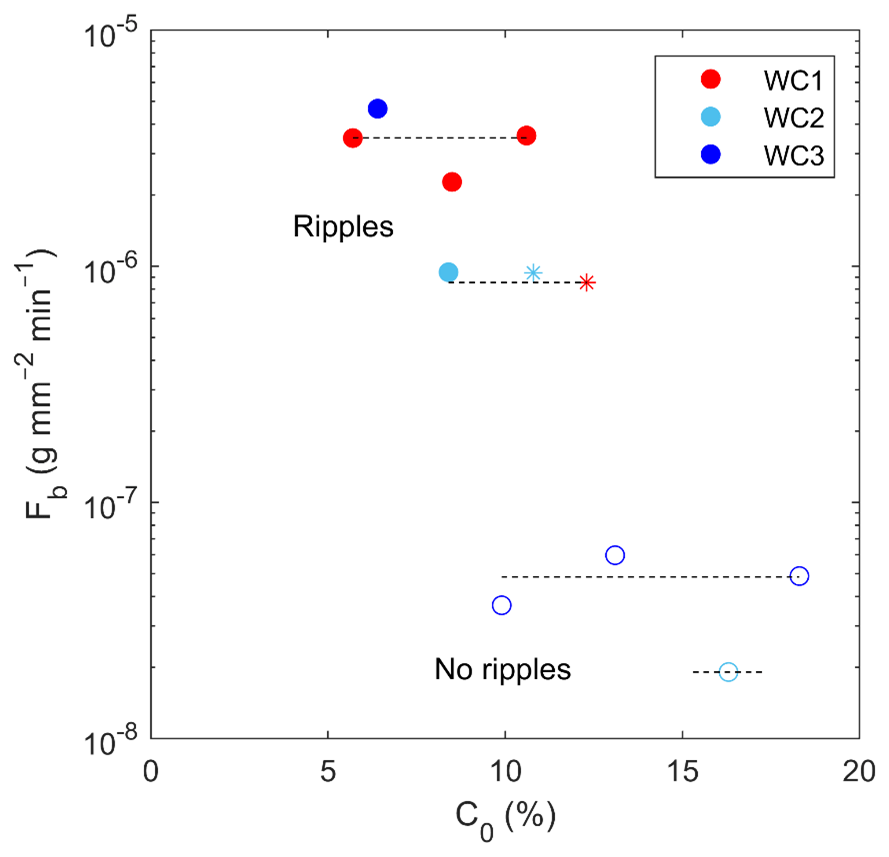
Figure 7 Average clay mass flux out of the bed, F_b, against initial clay content, C₀, for WC1 (red; Wu et al., 2022), WC2 (light blue), and WC3 (dark blue). Here solid circles, asterisks, and open circles signify large, small, and no ripples.

Ignoring changes in porosity and cohesion, the hydraulic conductivity is approximately proportional to $D_{\mathrm{10}\mathrm{m}}^{\mathrm{2}}$, where D_10m is the 10th percentile of the sand–clay mixture (Chapuis, 2012). For the mixture, there is little overlap in the sand and clay size distributions, D₅₀ ≫ D_50c, where D_50c is the median diameter of the clay particles (∼0.009 mm) and D₁₀= 0.34, 0.3, and 0.072 mm for the sand in the Wu et al. (2018), WC1–WC3, and Baas et al. (2013) cases. As C₀ increases, D_10m, and therefore the conductivity, will decrease gradually. However, when C₀ ≥ 10 %, D_10m switches from its approximate clean-sand value (∼D₁₀) to a much smaller size associated with the clay (∼D_50c), resulting in a reduction of 3 orders of magnitude for the Wu et al. (2018) and WC1–WC3 cases and 2 orders of magnitude for Baas et al. (2013). This reduction in hydraulic conductivity alone does not fully explain the behaviour seen in Fig. 7, as there are the effects of changes in permeability and erosion threshold to consider as well. However, it may be the reason for the drastic change in ripple steepness at C₀= 10.6 % for the Wu et al. (2018) and WC1–WC3 cases (Fig. 6a) and at the slightly higher value of C₀= 13 % for the Baas et al. (2013) cases, discussed in Sect. 4.1.

4.3 Enhanced threshold of motion

The phase diagram of Fig. 2 shows several cases without ripples (NR) (cf. Fig. 6a and Table 2), despite the skin friction being above the clean-sand threshold of motion (C₀≥ 16.3 % for WC2 and C₀≥ 9.9 % for WC3). The explanation for this discrepancy is that the clean-sand threshold of motion is enhanced by the presence of the clay. According to Whitehouse et al. (2000), for C₀≤ 30 % the enhanced threshold of motion can be expressed generically as

$$\begin{array}{}\text{(7)}& {\mathit{\theta }}_{\mathrm{0}\mathrm{E}}={\mathit{\theta }}_{\mathrm{0}}(\mathrm{1}+P_{\mathit{\theta }}{C}_{\mathrm{0}}),\end{array}$$

where P_θ is usually taken to be 20, but it can be anywhere within the range 6.7 $\le P_{\mathit{\theta }}\le$ 45. For WC1–WC3 and Wu et al. (2018), where D₅₀= 0.45 and 0.496 mm respectively, the clean-sand threshold is θ₀= 0.032. For combined colinear wave–current flow, the threshold line is described by ${\mathit{\theta }}_{\mathrm{0}\mathrm{E}}={\mathit{\theta }}_{\mathrm{w}}+{\mathit{\theta }}_{\mathrm{c}}$, where θ_c+θ_w is the maximum stress in the wave cycle. This results in the threshold line in Fig. 2 moving diagonally upward towards the upper right-hand corner with increasing C₀. If θ_0E for WC1–WC3 and Wu et al. (2018) is to be consistent with the bed characterizations (Tables 1, A1, and A3), it is necessary for θ_0E < θ_w+θ_c, when ripples are present (R), and θ_0E > θ_w+θ_c, when ripples are absent (NR). With P_θ= 20, for WC3 and C₀≥ 9.9 %, θ_0E≥ 0.095 > θ_w+θ_c, which is consistent with the R/NR bed characterizations. However, for WC2 and C₀= 16.3 %, θ_0E= 0.136 < θ_w+θ_c, which is inconsistent with its NR characterization (Table 1). Taking C₀= 16.3 % (WC2) as the limiting case, ${\mathit{\theta }}_{\mathrm{0}\mathrm{E}}={\mathit{\theta }}_{\mathrm{w}}+{\mathit{\theta }}_{\mathrm{c}}=$ 0.155, this gives a higher P_θ of 23 in Eq. (7) which restores consistency and is still within the range of Whitehouse et al. (2000). Figure 8a–f shows the magnitude of the time-varying skin friction using

$$\begin{array}{}\text{(8)}& \mathit{\theta }=\mathrm{|}{\mathit{\theta }}_{\mathrm{w}}\cos \mathit{\sigma }t+{\mathit{\theta }}_{\mathrm{c}}\mathrm{|},\end{array}$$

where σ= $\mathrm{2}\mathit{\pi }/T$, and the values of θ_w and θ_c are obtained from Tables 1, A1, and A3, compared with θ_0E using Eq. (7) with P_θ= 23 (yellow line). For all wave-only and wave–current cases, the above-threshold (rippled-bed) and below-threshold (flat-bed) cases are grouped together. Figure 8g shows the initiation time, t_i, when ripples begin to develop, from Tables 2, A1, and A3. In all cases, the skin friction is above threshold for only a fraction of the wave cycle. For each hydrodynamic condition, as the threshold increases with increasing C₀, these wave-cycle fractions above threshold decrease, with a corresponding increase in t_i (Fig. 8g), until the flat-bed cases, where the skin friction is always below threshold (Fig. 8e and f). In each below-threshold case there is an additional dashed line, which corresponds to the threshold based on the clay content at the end of the experiments (Fig. 5f, g, h and k). Apart from WC2 and C₀= 16.3 %, which is just above threshold at the end of the experiment (Fig. 8f), and WC3 and C₀= 6.4 %, which is just below threshold, by about the same amount (Fig. 8a), this new enhancement (P_θ= 23 in Eq. 7) is consistent with all combined wave–current and wave-only cases (Tables 1, A1, and A3).

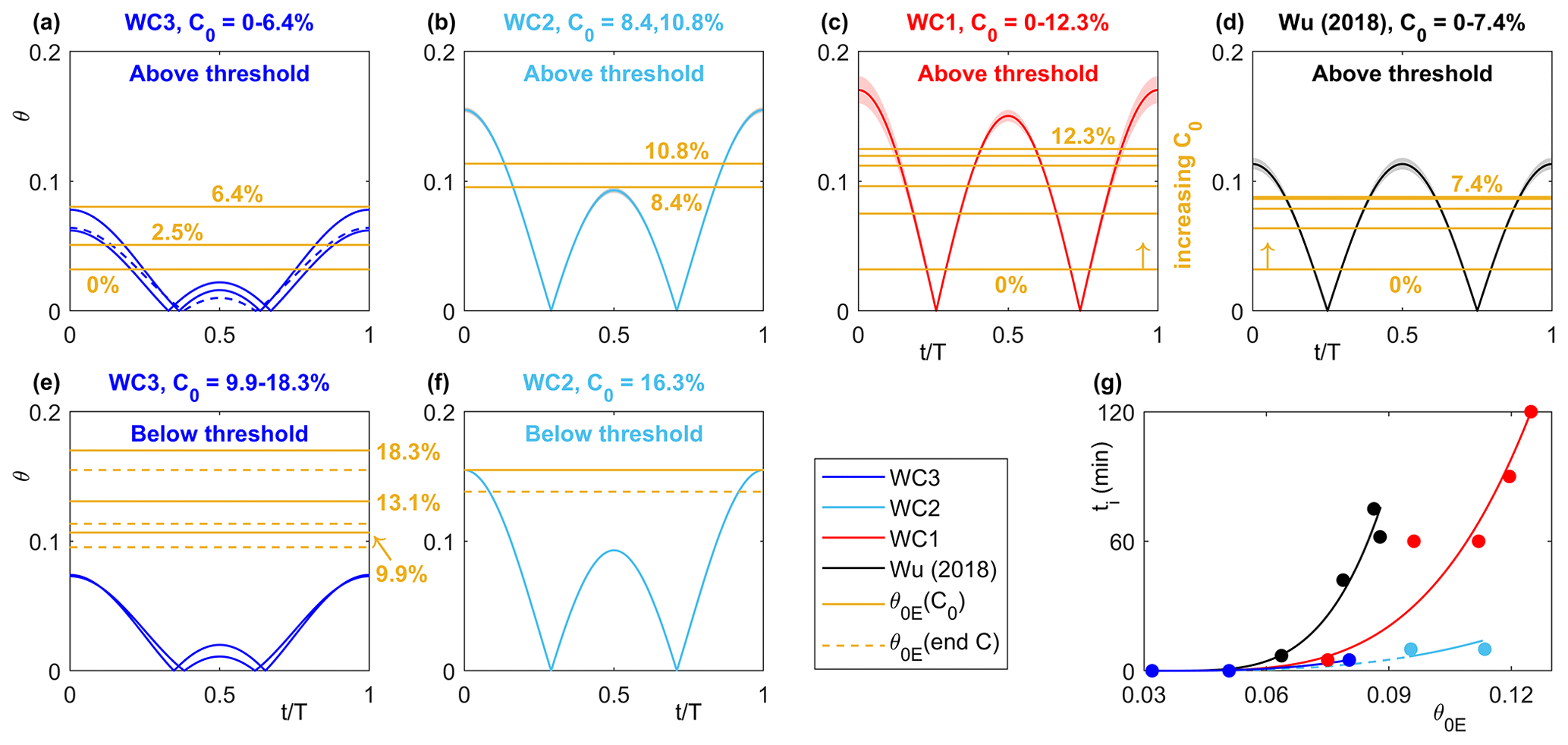
Figure 8 Time-varying skin friction using Eq. (8) compared to θ_0E using Eq. (7) with P_θ= 23, for the above- and below-threshold WC3 cases (a, e) and WC2 cases (b, f) and the above-threshold WC1 cases (c) and Wu et al. (2018) wave-only cases (d), as well as the initiation time, t_i, versus θ_0E (g), grouped according to flow condition. The legend applies to all panels. In (a) the dashed blue line corresponds to the C₀= 6.4 % case, in (c) and (d) the shaded region corresponds to the range of instantaneous skin friction values, and in (e) and (f) the below-threshold cases show an additional dashed line for θ_0E corresponding to the final sediment concentration.

In fine-sand, current-only experiments of Baas et al. (2013) (Table A2), runs with C₀≥ 5.4 % were below the enhanced threshold, θ_c < θ_0E, based on Eq. (7) with P_θ = 20. This is inconsistent with the observations as ripples appeared in these runs, indicating that this enhancement is too strong for D₅₀= 0.143 mm. Baas et al. (2019) found a far more modest threshold enhancement of P_θ= 3 in their threshold experiments for a similar grain size (D₅₀= 0.142 mm), where the velocity was stepped up sequentially over mixtures of sand and kaolinite clay until motion was detected. However, the enhancement of Baas et al. (2019) is a conservative estimate, since there was likely a cumulative effect of the sequential velocity steps, winnowing some of the clay from the bed before the threshold was passed for the sand grains. Figure 8 clearly shows that for the wave-only and wave–current cases, the initiation time is related to the fraction of the wave cycle when shear stresses are above threshold. However, the current-only cases are fundamentally different as a substantial initiation time infers that the bed must initially be below threshold. In the experiments of Baas et al. (2013), the C₀= 16.2 % and 18 % cases resulted in substantial initiation times (Table A2). Since the experiment with C₀= 13.8 % of Baas et al. (2013) did not have a substantial initiation time, it can be assumed to be above threshold. Taking the lowest θ_c for large ripples (C₀= 11.8 %) to represent the limiting case (θ_0E=θ_c); this gives P_θ= 6.4 in Eq. (7), which is close to the accepted range of Whitehouse et al. (2000) and is then consistent with all of the current-only experiments of Baas et al. (2013).

The critical shear stress enhancement for all mixed sand–kaolinite experiments can therefore be expressed as

$$\begin{array}{}\text{(9)}& {\mathit{\theta }}_{\mathrm{0}E}={\mathit{\theta }}_{\mathrm{0}}\times \left\{\begin{array}{ll}\mathrm{1}+\mathrm{6.4}{C}_{\mathrm{0}},& D_{\mathrm{50}}=\mathrm{0.143}\mathrm{mm},\\ \mathrm{1}+\mathrm{23}{C}_{\mathrm{0}},& \mathrm{0.45}\le D_{\mathrm{50}}\le \mathrm{0.50}\mathrm{mm},\end{array}\right.\end{array}$$

where θ₀= 0.061 for D₅₀= 0.143 mm and θ₀= 0.032 for 0.45 $\le D_{\mathrm{50}}\le$ 0.5 mm. Equation (9) states that there is a stronger enhancement of the threshold of motion for coarse sand compared to fine sand. This grain-size difference has been explained by van Rijn (2020) in terms of the clay content required to envelop a sand particle. Specifically, to completely envelop sand grains with a clay layer of thickness, d, the volumetric concentration of clay required can be expressed as an increasing function of $d/D_{\mathrm{50}}$. Therefore, for a given clay concentration, the ratio of d around the two sand sizes is given by $\mathrm{0.45}/\mathrm{0.143}$ ≈ 3. Interestingly, this ratio is similar to the ratio of constants in Eq. (9) for the two grain sizes. Thus, the thicker clay layer around the coarser grains likely causes increased enhancement of the threshold of motion, which has also been found in field observations (Harris et al., 2016). It can be expected that the Baas et al. (2021) field data, where D₅₀= 0.227 mm and 0.6 $\le C_{\mathrm{0}}\le$ 5.4 %, should have a coefficient somewhere between 6.4 and 23. The coefficient would probably be closer to 6.4, as there was no obvious change in the threshold during the field campaign. However, it is difficult to be more specific as the dominant clay mineral in the sediment was illite rather than kaolinite, and there is also the presence of extracellular polymeric substances (EPS) to consider (Malarkey et al., 2015; Baas et al., 2019).

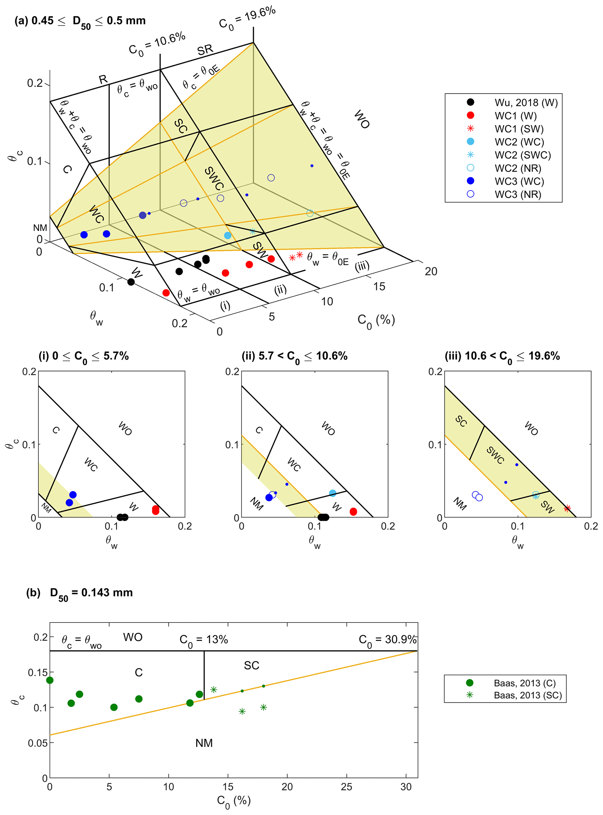
Figure 9 Orthographic projection of the 3D phase diagram with clay dependence for 0.45 $\le D_{\mathrm{50}}\le$ 0.50 mm (a) and 2D C₀−θ_c plot for D₅₀= 0.143 mm (b), with the enhance critical shear stress, θ_0E, based on Eq. (9), represented as the yellow surface. Below-threshold cases have appropriately coloured small dots to mark the critical shear stress on the surface. In (a) there are also three 2D cross sections viewed from the C₀= 0 % end: (i) 0 ≤C₀ ≤ 5.7 % (ii) 5.7 < C₀≤ 10.6 %, and (iii) 10.6 < C₀≤ 19.6 %, marked in the 3D plot. Solid circles: large ripples (R), asterisks: small ripples (SR), open circles: no ripples (NR), C: current-dominant, WC: wave–current, W: wave-dominant (S prefix in SC and SWC for small ripples), NM: no motion, and WO: washout.

4.4 Bedform phase diagrams

As proposed by Schindler et al. (2015), clay content can be incorporated into 3D phase diagrams. This has been done in Fig. 9a and b by making use of Eq. (9) and separating all the data depicted in Fig. 2 into the two different grain-size ranges: 0.45 $\le D_{\mathrm{50}}\le$ 0.5 mm and D₅₀= 0.143 mm (for the latter case only the current shear stress axis is shown as there is insufficient data for the full 3D plot). In this new 3D phase diagram framework, there are four main regions: no motion (NM), ripples (R), small ripples (SR), and washed-out ripples (WO). The upper boundary of NM is the yellow surface described by ${\mathit{\theta }}_{\mathrm{w}}+{\mathit{\theta }}_{\mathrm{c}}={\mathit{\theta }}_{\mathrm{0}\mathrm{E}}$, where θ_0E is given by Eq. (9), such that θ_0E= θ₀ when C₀= 0 %. The NM region gradually expands with increasing C₀. This expanding region means the threshold eventually reaches the washout limit, θ_0E=θ_wo, where the ripple height starts to decrease near sheet flow conditions. Here, θ_0E=θ_wo corresponds to C₀= 19.6 %, for 0.45 $\le D_{\mathrm{50}}\le$ 0.5 mm, and C₀= 30.9 %, for D₅₀= 0.143 mm, which is broadly consistent with the lower limit of Whitehouse et al. (2000) of between 20 % and 30 % for cohesive erosion in mixtures of sand and clay.

In Fig. 9a, the large and small ripple regions are each subdivided into three subregions: wave-dominant (W and SW; θ_c < 0.2θ_w), wave–current (WC and SWC; 0.2θ_w < θ_c < 3.3θ_w), and current-dominant (C and SC; θ_c > 3.3θ_w). The C/SC subdivision is shown in Fig. 9b. Figure 9a also shows 2D cross sections viewed from the C₀= 0 % end: (i) 0 $\le C_{\mathrm{0}}\le$ 5.7 %, (ii) 5.7 < C₀≤ 10.6 %, and (iii) 10.6 < C₀≤ 19.6 %, marked in the 3D plot for reference. In Fig. 9b for D₅₀= 0.143 mm, the small current ripples for C₀= 16.2 % and 18 % appear in the NM region because it is thought that these cases were initially below threshold, as explained in Sect. 4.3. It is also likely that these ripples had not reached equilibrium (Table A2; Baas et al., 2013). This illustrates the point that this phase diagram is dynamic: even if the flow conditions place the data in the no movement region for sand, or indeed the washout region, clay can still be winnowed out of the bed as it was in some of the WC3 and WC2 cases (Fig. 5f, g, h, and k).

5 Implications for palaeowave climate predictions and bedform phase diagrams

The reduction in ripple wavelength with increasing C₀, and specifically how it relates to the orbital diameter through Eq. (6), may have consequences for palaeoenvironmental reconstruction. Based on orbital ripples preserved in the rock record, Diem (1985) used α= 0.65 to determine the orbital diameter and hence the palaeowave climate, which included water depth and wave height and period. Thus, it is likely that if α is lowered by the presence of clay this would underpredict the ancient orbital diameter, resulting in inaccurate palaeowave climate predictions.

The predictions of the new 3D phase diagram framework show a dramatic reduction in bedform size and therefore form roughness, which is proportional to ${\mathit{\eta }}^{\mathrm{2}}/\mathit{\lambda }$ (Soulsby, 1997). In the specific case of the intertidal field site in the Dee Estuary of Baas et al. (2021), on which the 2D phase diagram (Fig. 2) is based, there were no instances of smaller flatter ripples, which is consistent with the range of C₀ measured: 0.6 $\le C_{\mathrm{0}}\le$ 5.4 %. However, considering the widespread occurrence of mixed sand and mud flats (Murray et al., 2019), the scenario that an increase in the threshold shear stress in the presence of clay significantly affects the state of the bed could occur frequently. Thus, it is likely that ripple dimensions could have been commonly overestimated by existing ripple predictors, potentially affecting the performance of morphodynamic models. The applicability of these 3D phase diagrams therefore requires further testing in muddy environments.

6 Conclusions

The present experiments examined ripple dynamics on cohesive beds under two different combined wave–current conditions with initial clay content, C₀, ranging from 0 % to 18.3 %. For the lowest C₀, these experiments produced quasi-asymmetric ripples, which are similar to their clean-sand counterparts, with equilibrium heights and wavelengths within the ranges 13.9 $\le {\mathit{\eta }}_{\mathrm{e}}\le$ 15 mm and 137 $\le {\mathit{\lambda }}_{\mathrm{e}}\le$ 148 mm respectively, with the larger values corresponding to the strongest relative current. For higher C₀, smaller flatter ripples that were fully asymmetric, with η_e= 5.6 mm and λ_e= 125 mm, were produced. Finally, for the highest C₀, no ripples were produced and the bed remained flat.

Combining the present experiments with previous wave-only and wave–current experiments (Wu et al., 2018, 2022) demonstrates the existence of a large to small equilibrium ripple discontinuity at C₀= 10.6 %, with two distinct ripple steepness (RS) groupings, RS ≥ 0.09 and RS ≈ 0.04, which is probably related to a decrease of 3 orders of magnitude in the hydraulic conductivity. The larger RS grouping shows a decrease from 0.14 to 0.1 with increasing current strength. Ripple wavelength was independent of initial clay content for C₀≤ 7.4 %, but it decreased linearly with initial clay content for C₀ > 7.4 %. For C₀≤ 7.4 %, the wavelength was proportional to the current-enhanced orbital diameter, d_wc, so that λ_e= αd_wc, where α= 0.61. For C₀ > 7.4 %, α decreased linearly, which could be important for palaeoenvironment reconstruction, when λ_e is measured and d_wc is unknown. During the experiments, clay winnowing removed clay from both the active layer (crest to trough) and deep beneath it, in the case of most large ripples. Winnowing was quantified by the average mass flux of clay out of the bed over the duration of the experiment. Winnowing still occurred from flat beds, but compared to the large ripples the flux was typically 2 orders of magnitude smaller.

The ripple initiation time increased with initial clay content, and ultimately the bed remained flat when the initial clay content was large enough, demonstrating the enhancement of the threshold of sediment motion with increased initial clay content. When combined with the fine-sand current-only experimental results of Baas et al. (2013), this allowed the enhancement of the threshold to be quantified for both coarse (0.45 ≤ D₅₀≤ 0.5 mm) and fine (D₅₀= 0.143 mm) mixed sand–clay motion. On the basis of these enhancements, new 3D phase diagrams, involving the non-dimensional wave and current shear stresses and C₀, are proposed to characterize the two ripple size groupings under different flow conditions. This new 3D phase diagram framework should prove important to the morphodynamic modelling community.

Appendix A: Experimental conditions of Wu et al. (2022), Baas et al. (2013) and Wu et al. (2018).

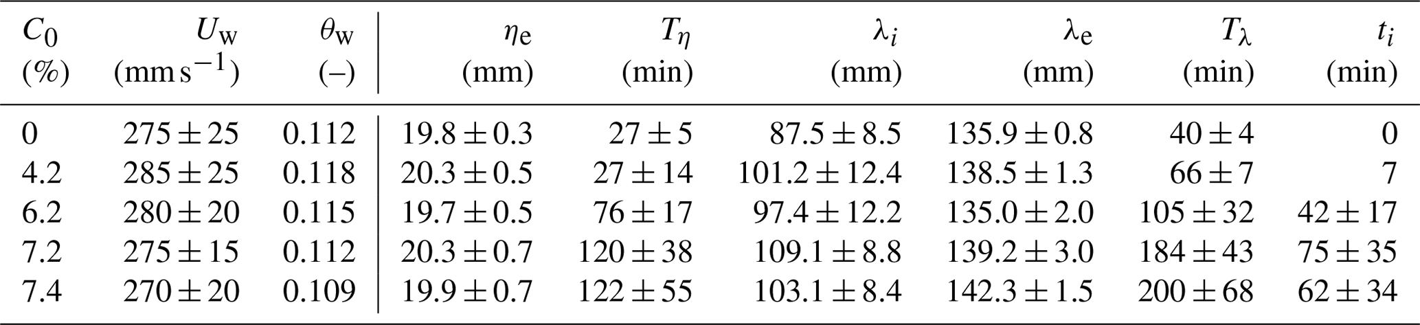
Table A1 Wave–current experiments of Wu et al. (2022), where h= 400 mm, T= 2 s, D₅₀= 0.45 mm, ν= 1.12 mm² s⁻¹, and ρ= 1000 kg m⁻³, referred to in the main text as WC1 (θ₀= 0.032). Bedforms developed in all cases (R). ^* This fit is based on fitting two stages to the growth (see Wu et al., 2022).

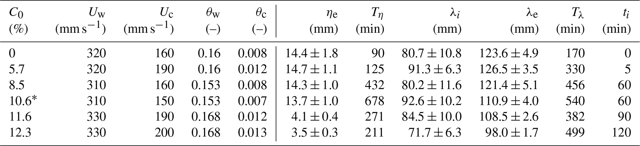
Table A2 Current-only experiments of Baas et al. (2013), with U_w= 0 mm s⁻¹ (θ_w= 0), D₅₀= 0.143 mm, ν= 1.02 mm² s⁻¹, and ρ= 1000 kg m⁻³ (θ₀= 0.061). Bedforms developed in all cases (R). ^* Equilibrium not reached after 2 h.

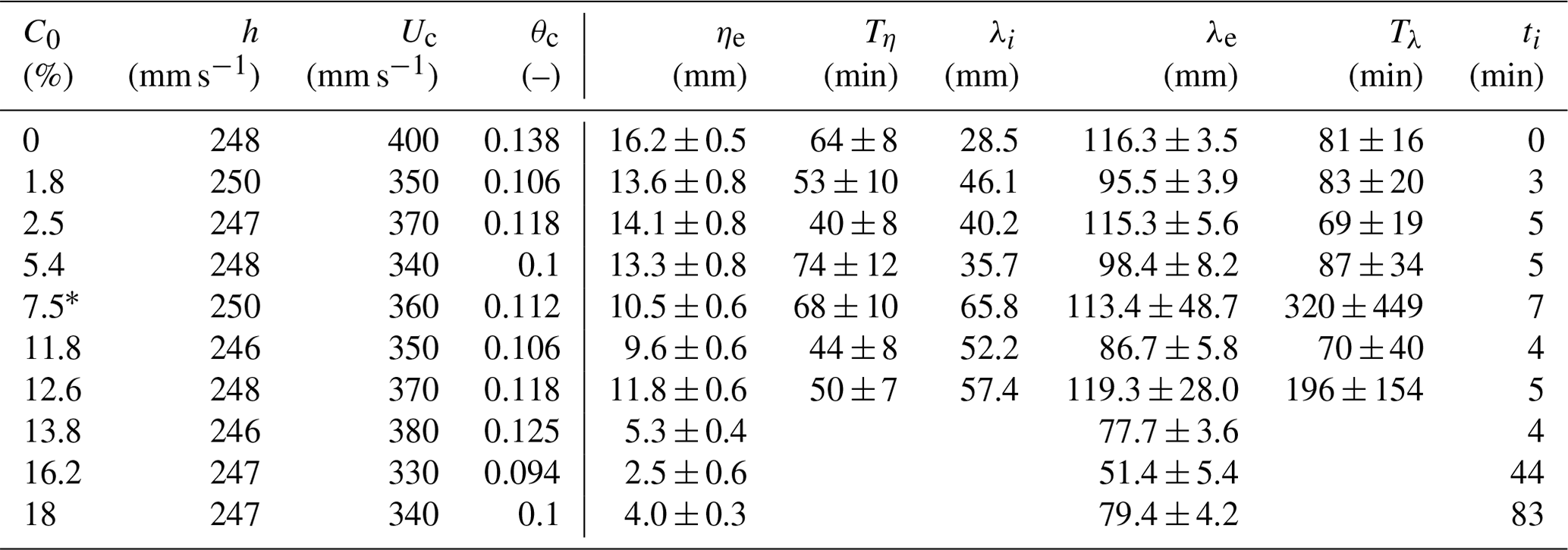
Table A3 Wave-only experiments of Wu et al. (2018), with U_c= 0 mm s⁻¹ (θ_c= 0), h= 600 mm, T= 2.48 s, D₅₀= 0.496 mm, ν= 1.14 mm² s⁻¹, ρ= 1015 kg m⁻³, and U_w= (U_won+U_woff)$/\mathrm{2}$ ± (U_won−U_woff)$/\mathrm{2}$, where U_won and U_woff are the onshore and offshore freestream velocities (θ₀= 0.032). Bedforms developed in all cases (R).

Appendix B: Determining the effective orbital diameter under combined flow

For a colinear sinusoidal wave and current, the horizontal velocity close to the bed is

$$\begin{array}{}\text{(B1)}& u_{\mathrm{wc}}=U_{\mathrm{w}}(\cos \mathit{\phi }+b),\end{array}$$

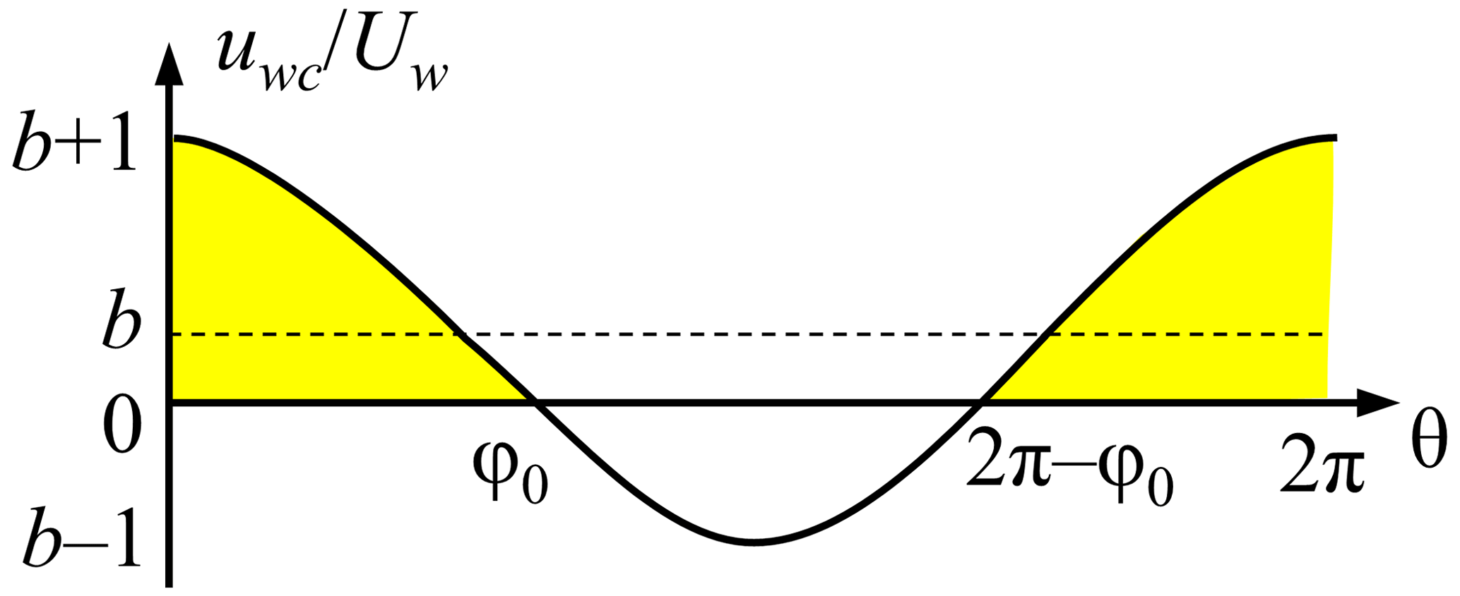
where φ=σt is the phase of the wave, σ= 2$\mathit{\pi }/T$, t is time, b= $A{U}_{\mathrm{c}}/U_{\mathrm{w}}$, and A is constant (A < 1 as the near-bed current will be less than the depth-averaged current velocity). Figure B1 shows Eq. (B1) graphically. The orbital diameter, which is the horizontal distance moved between the two flow reversals for the positive wave half cycle, is shown by the shaded area under the curve. The zero-crossing phase is given by

$$\begin{array}{}\text{(B2)}& {\mathit{\phi }}_{\mathrm{0}}=\arccos [max(-b,-\mathrm{1}\left)\right].\end{array}$$

When b≥ 1, φ₀=π; there are no zero crossings, and only a single minimum. The effective orbital diameter, d_wc, corresponding to the shaded area in Fig. B1 is

$$\begin{array}{}\text{(B3)}& d_{\mathrm{wc}}=\mathrm{2}\mathit{\sigma }{\int }_{\mathrm{0}}^{{\mathit{\phi }}_{\mathrm{0}}}{u}_{\mathrm{wc}}d\mathit{\phi }=d_{\mathrm{0}}(\sin {\mathit{\phi }}_{\mathrm{0}}+b{\mathit{\phi }}_{\mathrm{0}}),\end{array}$$

where $d_{\mathrm{0}}=U_{\mathrm{w}}T/\mathit{\pi }$ (Soulsby, 1997) is the wave-only orbital diameter for the wave alone, when b= 0. For the wave–current experiments, the value of A used in the parameter b was A= 0.1, 0.22, and 0.42 for WC1, WC2, and WC3 respectively; for the wave-only Wu et al. (2018) experiments, d_wc =d₀ since b= 0.

Figure B1 Plot of Eq. (B1), where shaded area represents d_wc in Eq. (B3).

Appendix C

Nomenclature
C Measured core clay content	ηe Equilibrium ripple height
C0 Initial clay content	ηt Mean ripple height at time t
Cdef Clay deficit ($=C_{\mathrm{0}}-C$)	θ Instantaneous Shields parameter
D* Dimensionless grain size	θ0 Clean-sand threshold Shields parameter
D10 10th percentile of sand	θ0E Enhanced threshold Shields parameter
D10m 10th percentile of sand–clay mixture	θc Current-only Shields parameter
D50 Median grain size of sand	θrms Root-mean square of θ
D50c Median grain size of clay	θw Wave-only Shields parameter
dc Equivalent clean-sand depth ($=I/C_{\mathrm{0}})$	θwo Washout Shields parameter
dwc Current-enhanced orbital diameter	λ Ripple wavelength
Fb Average mass flux of clay out of bed	λe Equilibrium ripple wavelength
g Acceleration due to gravity	λl Length of ripple lee side
H Wave height	λs Length of ripple stoss side
h Water depth	λt Mean ripple wavelength at time t
I Total amount of clay removed from bed	ν Kinematic viscosity of water
T Wave period	ρ Water density
Tη Equilibrium time for ripple height	ρs Sediment density
Tλ Equilibrium time for ripple wavelength	τc Current-only skin friction
t Bed scanning time	τw Wave-only skin friction
td Duration of experiment
ti Time of first appearance of ripples
Uc Depth-average current velocity	Abbreviations
Uw Wave velocity amplitude	NM No movement
u* Shear velocity scale	NR No ripples
z Vertical position relative to crest	RS Ripple steepness ($={\mathit{\eta }}_{\mathrm{e}}/{\mathit{\lambda }}_{\mathrm{e}})$
α Constant of proportionality	RSI Ripple symmetry index ($={\mathit{\lambda }}_{\mathrm{s}}/{\mathit{\lambda }}_{\mathrm{l}}$)
η Ripple height	WO Washout