the Creative Commons Attribution 4.0 License.
the Creative Commons Attribution 4.0 License.
 | 29 Apr 2024
On the relative role of abiotic and biotic controls in channel network development: insights from scaled tidal flume experiments
Sarah Hautekiet
Jan-Eike Rossius
Olivier Gourgue
Maarten Kleinhans
Stijn Temmerman
Tidal marshes provide highly valued ecosystem services, which depend on variations in the geometric properties of the tidal channel networks dissecting marsh landscapes. The development and evolution of channel network properties are controlled by both abiotic (dynamic flow–landform feedbacks) and biotic processes (e.g. vegetation–flow–landform feedbacks). However, the relative role of biotic and abiotic processes, and under which condition one or the other is more dominant, remains poorly understood. In this study, we investigated the impact of spatio-temporal plant colonization patterns on tidal channel network development through flume experiments. Four scaled experiments mimicking tidal landscape development were conducted in a tidal flume facility: two control experiments without vegetation, a third experiment with hydrochorous vegetation colonization (i.e. seed dispersal via the tidal flow), and a fourth with patchy colonization (i.e. by direct seeding on the sediment bed). Our results show that more dense and efficient channel networks are found in the vegetation experiments, especially in the hydrochorous seeding experiment with slower vegetation colonization. Further, an interdependency between abiotic and biotic controls on channel development can be deduced. Whether biotic factors affect channel network development seems to depend on the force of the hydrodynamic energy and the stage of the system development. Vegetation–flow–landform feedbacks are only dominant in contributing to channel development in places where intermediate hydrodynamic energy levels occur and mainly have an impact during the transition phase from a bare to a vegetated landscape state. Overall, our findings suggest a zonal domination of abiotic processes at the seaward side of intertidal basins, while biotic processes have an additional effect on system development more towards the landward side.
- Article
(13656 KB) - Full-text XML
-
Supplement
(50316 KB) - BibTeX
- EndNote


Tidal wetlands are valuable coastal ecosystems providing numerous ecosystem services such as shoreline protection and carbon sequestration (Allen, 2000; Barbier et al., 2011; Leonardi et al., 2018; Mcowen et al., 2017; Rogers et al., 2019). The landscape is dissected by tidal channel networks, which play a key role in the ecosystem functioning since channels act as major flow paths for water, nutrients, sediments, and biota (Fagherazzi et al., 1999, 2012; Huiskes et al., 1995; Kearney and Fagherazzi, 2016; Temmerman et al., 2007; Vandenbruwaene et al., 2012). The geometric properties of the channel networks (e.g. density of channelization, channel width, depth, and cross-sectional area) can widely vary within tidal marsh systems both locally and globally. Understanding these spatial variations in geometric properties is essential as they may imply variability in the ecosystem functioning and associated ecosystem services of tidal marshes. For instance, it has been shown that (1) the depth of subsurface groundwater fluctuations varies with distance from channels (Ursino et al., 2004; Van Putte et al., 2020), and hence related processes such as vegetation zonation, rates of carbon sequestration, and nutrient cycling in marsh sediments also vary as a function of distance from channels and thus channel drainage density (Krask et al., 2022; Roner et al., 2016; Xin et al., 2022); (2) marsh resilience to sea level rise depends on sediment accretion rates which also vary as a function of distance from channels (D'Alpaos et al., 2007; Fagherazzi et al., 2012; Kirwan et al., 2008; van Dobben et al., 2022); and (3) storm surge attenuation is less effective when marshes have wider, deeper, and denser channel networks (Stark et al., 2016; Temmerman et al., 2012, 2023).
Abiotic and biotic processes actively shape the tidal landscape and affect the geometric properties of channel networks. Tidal channels develop due to abiotic feedback between spatial heterogeneity in topography and/or sediment erodibility, on the one hand, and tidal flow and erosion patterns, on the other hand. Once initial depressions form by spatial heterogeneity, flow converges to these depressions, initiating channel formation (D'Alpaos et al., 2006; Kleinhans et al., 2009; Stefanon et al., 2010). The evolution of these channels is typically driven by headward erosion (Kleinhans et al., 2012; D'Alpaos et al., 2005; Stefanon et al., 2010), which is mainly induced by ebb currents (Geng et al., 2020). Such channels are ebb-dominant in the unvegetated state, meaning that the landward fluxes of sediment, nutrients, and biota remain limited (Kleinhans et al., 2009; D'Alpaos et al., 2005; Mariotti and Fagherazzi, 2011). But once vegetation has settled alongside the channels, the tides within the channels are more symmetrical, allowing sediment trapping (Kleinhans et al., 2009; Stark et al., 2017). In the past few decades, geometric features of tidal wetlands have been extensively investigated, revealing an abiotic relation between tidal prism and channel cross-sectional area, not only for tidal inlets (e.g. Byrne et al., 1980; Jarrett, 1976; Myrick and Leopold, 1963) but also explaining variations in channel cross-sectional areas within channel networks of tidal wetlands (D'Alpaos et al., 2010; Rinaldo et al., 1999b). Furthermore, spatial variations in geometric properties of marsh channel networks were found to be related to the respective tidal watershed area (D'Alpaos et al., 2010; Marani et al., 2003; Rinaldo et al., 1999a, b).
Biotic factors affect the landscape configuration of tidal wetlands through feedback between plants, water flow, and sediment (Bouma et al., 2013; Temmerman et al., 2005, 2007; Vandenbruwaene et al., 2013). Vegetation slows down flow velocity locally within patches (Zong and Nepf, 2010, 2011, 2012; Ortiz et al., 2013; Meire et al., 2014) and triggers the initiation of channel formation by flow acceleration next to and in between vegetation patches (Schwarz et al., 2014; Temmerman et al., 2007; Vandenbruwaene et al., 2015). The resulting landscapes have a higher density of channelization (Vandenbruwaene et al., 2013) and more efficiently draining channel networks in comparison to unvegetated landscapes, as larger portions of marsh platforms are closer to a channel (Kearney and Fagherazzi, 2016). Moreover, life history traits, such as plant recruitment strategies, can influence wetland geomorphology and channel network characteristics (Bij de Vaate et al., 2020; Schwarz et al., 2018, 2022). Specifically, a slow patchy colonization pattern seems to enhance the formation of new channels. In contrast, a fast homogeneous colonization pattern tends to favour stabilization of pre-existing channels, leading to a lower density of channel networks (Schwarz et al., 2018, 2022).
Both abiotic and biotic controls on tidal channel formation and evolution have been identified, but the relative role of abiotic and biotic factors, and under which conditions one or the other is more dominant, remains poorly understood. We suspect this is partly because tidal channel networks develop over large spatial (∼ km2) and temporal scales (∼ decades), while biota and their patterns have much smaller scales. Furthermore, subtle differences in gradual marsh vegetation development, caused by different life history traits, might cumulatively lead to large-scale, long-term effects on tidal channel network development. Present insights mainly come from either numerical models simulating tidal channel network development over such large spatial scales and timescales as a result of plant–flow–sediment feedbacks (D'Alpaos et al., 2007; Gourgue et al., 2022; Kirwan and Murray, 2007; Schwarz et al., 2018), which have the disadvantage that they may ignore real-life processes, or empirical analyses of tidal channel geometric properties from different wetland sites (Kearney and Fagherazzi, 2016; Kleinhans et al., 2009; Liu et al., 2022; Vandenbruwaene et al., 2013), which have the drawback that site-specific conditions that may have affected the channel development are not necessarily known and difficult to control. Experimental studies, which enable the isolation of abiotic and biotic effects (e.g. by repeated experiments with and without vegetation), are practically impossible on the relevant spatial (∼ km2 ) and temporal scales (∼ decades) unless they are scaled.
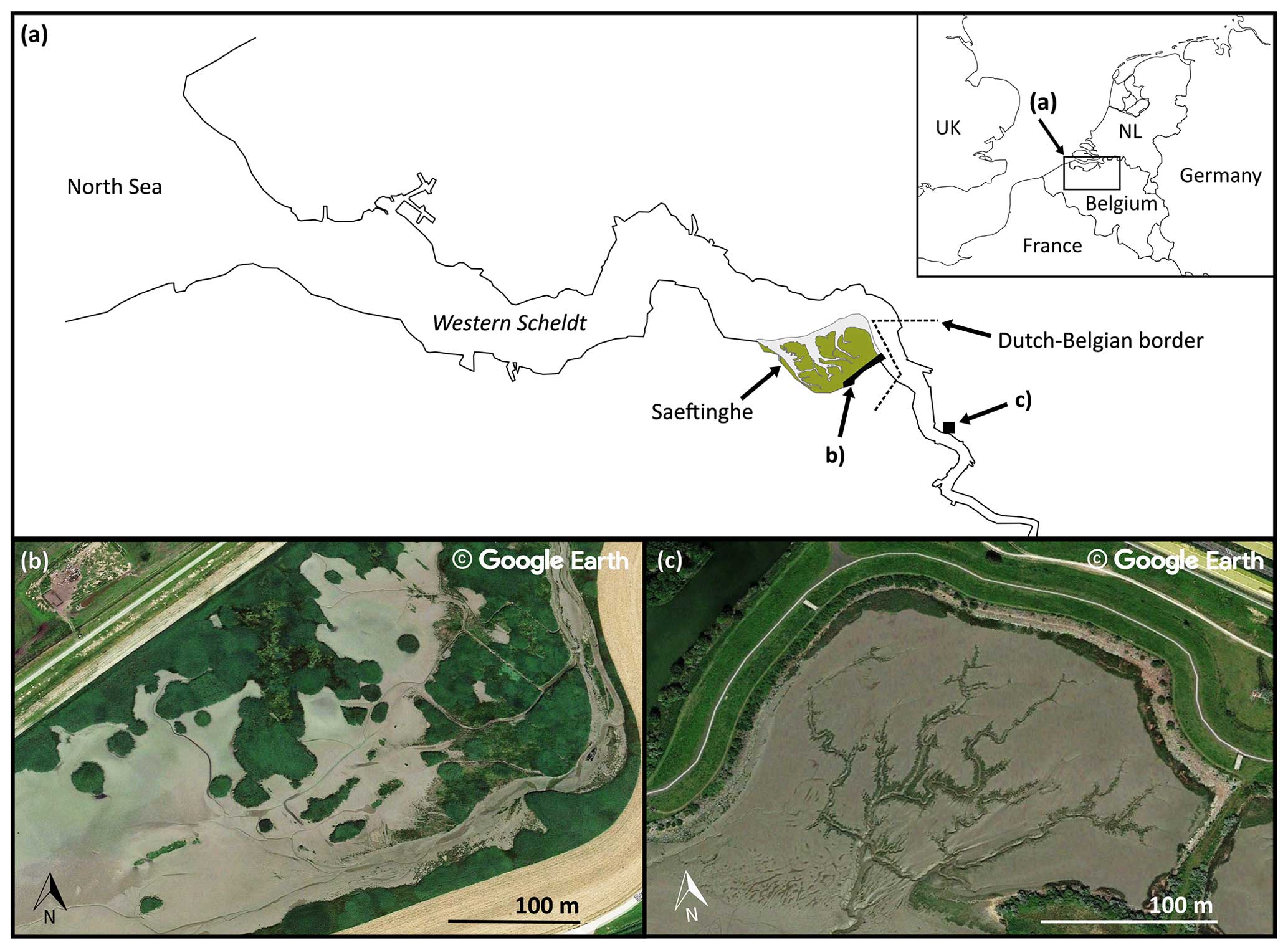
Figure 1(a) Overview of two example sites along the Scheldt estuary (N Belgium and SW Netherlands) where patchy and hydrochorous plant colonization patterns can be found: (b) the Sieperda marsh (NL), showing a patchy colonization strategy, and (c) the Lillo-Potpolder (BE), exhibiting a hydrochorous colonization strategy. The satellite imagery was extracted from © Google Earth 2013 (image of the Sieperda marsh) and © Google Earth 2021 (image of the Lillo-Potpolder).
In general, scaled laboratory experiments have been used to study the formation and evolution of fluvial and tidal landscapes with live vegetation in a simplified setting (Kleinhans et al., 2015a; Tal and Paola, 2007; Piliouras et al., 2017; Piliouras and Kim, 2019a, b; Zhou et al., 2014). Nevertheless, few morphodynamic experiments with tides have been conducted due to issues with scale effects (e.g. Stefanon et al., 2010; Tambroni et al., 2005; Vlaswinkel and Cantelli, 2011). Recent advances made in scaled tidal morphodynamic experiments, in particular using flumes with a tilting bed to generate tidal flow, allow for overcoming the most limiting scale effects and developing realistic estuarine morphologies (Kleinhans et al., 2012, 2017b, 2015b). So far, most flume experiments comparing bare and vegetated tidal systems have been carried out in an estuarine context (i.e. with a landward river discharge boundary and seaward tidal boundary) and indicate that vegetation can influence the morphological development of partially filled estuaries (Kleinhans et al., 2022; Weisscher et al., 2022). These experiments showed that vegetation confines the flow into channels and reduces both channel mobility and local flow velocity, ultimately contributing to bar stabilization and further infilling of the estuary. To our knowledge, experiments have not been conducted yet with a focus on (1) channel network development in an intertidal basin context (i.e. only seaward tidal boundary and closed landward boundary) and (2) the role of vegetation presence or absence and colonization patterns in the resulting channel network geometric properties.
In this study, we aim to advance our understanding of the relative roles of abiotic and biotic effects in the development of landward-branching, blind-ending tidal channel networks within intertidal basins through novel flume experiments. Specifically, we investigate the impact of three different spatio-temporal plant colonization strategies on channel network formation: (1) a control without plant colonization, (2) hydrochorous colonization, and (3) patchy colonization (see Fig. 1). The hydrochorous colonization experiment represents certain aspects of tidal wetland systems dominated by annual (e.g. Salicornia spp.) and biennial (e.g. Aster spp.) pioneer plants producing many seeds that typically disperse hydrochorously with the tidal flow (Gray, 1971; Davy et al., 2001; Huiskes et al., 1995). The patchy colonization experiment, on the other hand, represents systems dominated by slowly colonizing perennial plants (e.g. Scirpus or Spartina spp.), which reproduce clonally, thereby developing gradually expanding vegetation patches (Bouma et al., 2007; Schwarz et al., 2018, 2022; Vandenbruwaene et al., 2011). We hypothesize that the patchy recruitment strategy will be associated with local flow deceleration within vegetation patches and flow acceleration next to expanding patches. Hence, it might enhance channel formation and result in higher channel density compared to the scenario without plant colonization. The hydrochorous recruitment strategy may show a more homogenous spatial recruitment pattern. Therefore, it might generate less local flow concentration and thus produce less dense channel networks. The effect of vegetation is hypothesized to be most relevant during the transition phase from bare to vegetated intertidal wetlands, after which the system is expected to evolve toward a morphodynamic equilibrium.
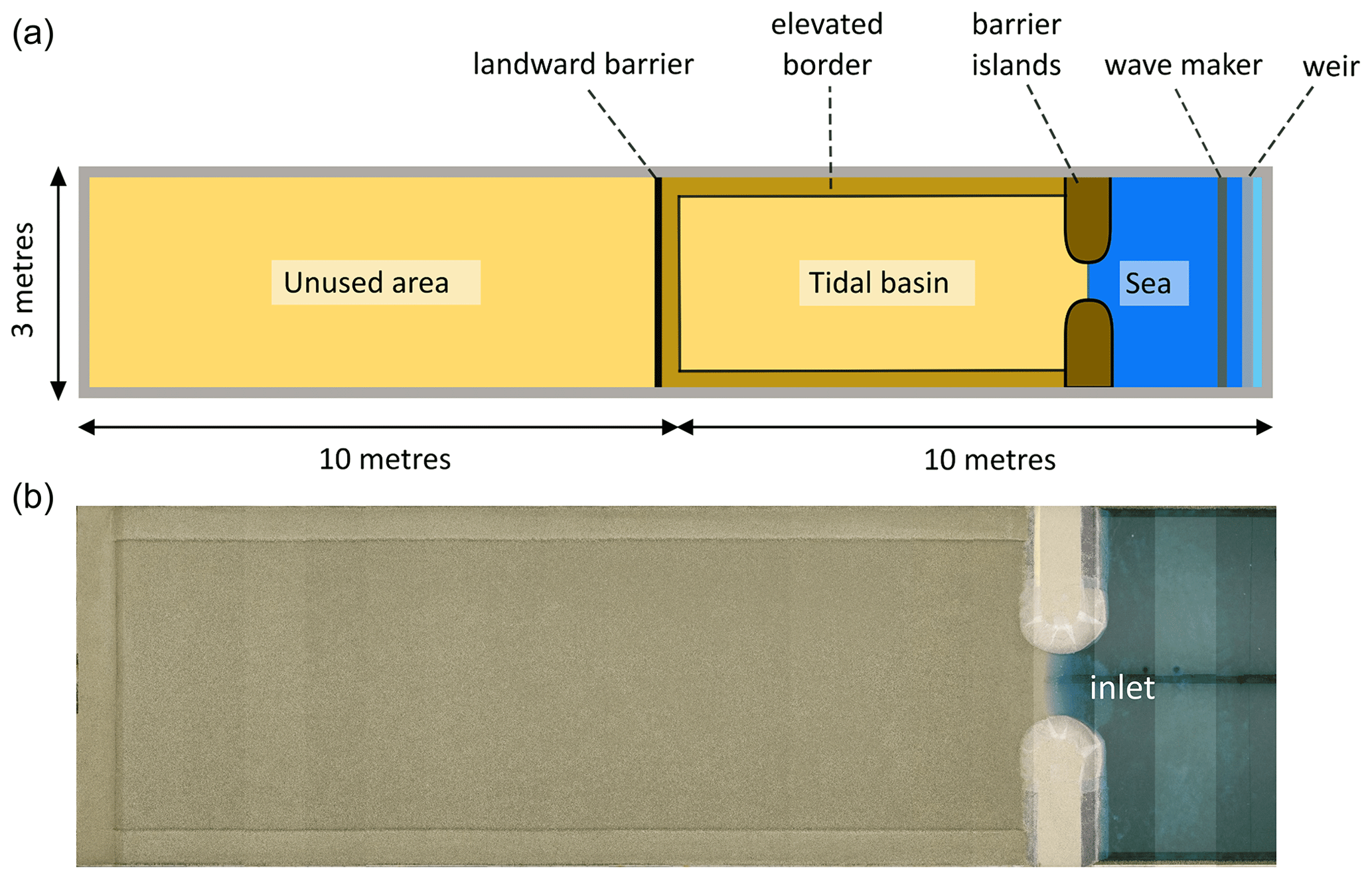
Figure 2Top-view sketch (a) and overhead photograph mosaic (b) of the experimental set-up of the flume showing features such as the tidal basin, elevated borders along the tidal basin, the landward barrier of the tidal basin, the sea basin, and barrier islands adjacent to the tidal inlet connecting the sea and tidal basin.
2.1 Experimental set-up and procedure
Four landscape-scale experiments of salt marshes were conducted in the Metronome tidal facility at Utrecht University: two control experiments without vegetation (only sand), a third experiment with hydrochorous seeding of vegetation, and a fourth with patchy seeding. Initial conditions and general settings were the same for all four experiments, and only the presence or absence of vegetation and the type of vegetation seeding were different (see Sect. 2.2).
The Metronome is a 20 m long and 3 m wide box-shaped flume where tides are generated by periodically tilting the construction over the short central axis (Kleinhans et al., 2017b). It has been designed to overcome scale problems observed in previous scaled morphodynamic studies of tidal landscapes (e.g. Stefanon et al., 2010). A complete overview of the design and functioning of the flume can be found in Kleinhans et al. (2017b). For the current experiments, a 7.4 m long and 2.4 m wide zone, acting as an intertidal basin, was created and filled with an 11.5 cm thick sand bed (Fig. 2). It was bordered by two fixed non-erodible barrier islands connecting the intertidal basin with the “sea basin”, which initially had no sand bed but just the fixed flume bottom. The barrier islands (each 50 cm wide, ±1.23 m long, and 25 cm high) were installed to create a 55 cm wide tidal inlet. We decided to use fixed barriers to avoid interference with the flume walls and to create a branching channel network similar to the results obtained by Kleinhans et al. (2012). These barriers consisted of a wooden framework with inclined sides and sandy round heads. Their entire exterior was covered in bubble wrap to have a uniform surface with increased hydraulic roughness.
Furthermore, a landward barrier along the complete width of the tidal basin was created to confine the system. The 30 cm wide borders of the tidal basin were slightly elevated at 14.5 cm (Fig. 2). The initial bed, including elevated borders, was levelled and consisted of poorly sorted sand with a median grain size d50=0.55 mm, d10=0.32 mm, and d90=1.2 mm.
The experiments were run for 5000 (first control experiment), 5500 (hydrochorous vegetation experiment), and 10 000 tidal cycles (second control and patchy vegetation experiment), respectively. These numbers correspond to about 7, 8, and 14 years of natural tidal cycles in case of a semi-diurnal tidal regime. As every tidal cycle in the Metronome takes 40 s, the experiments took 5 and 10 d to run for the first and second control experiment, respectively. The vegetated experiments took longer to run as we had to wait 4 d between sowing events for seeds to germinate and grow sprouts. They both took around 1.5 months (±50 d) to run. The selected experimental settings were based on 12 pilot experiments (all without inclusion of vegetation) in which settings such as sea level and tidal inlet width were varied until a dendritic channel network was created while avoiding interference with the flume walls.
Tidal asymmetry was imposed on the tilting flume to create a flood-dominant system. A principal tide (M2) was generated with a period of 40 s at an amplitude of 75 mm, while the overtide (M4) had an amplitude of 15 mm (i.e. 20 % of M2 component) over a period of 20 s. This resulted in a maximum slope of 0.009 m m−1 during flood and a maximum slope of 0.006 m m−1 during ebb. These conditions are similar to those in Weisscher et al. (2022), where the tidal asymmetry limited net seaward export of sediment observed in most tidal experiments in the literature. At the seaward end, waves were generated by a horizontal paddle with a frequency of 2 Hz during the flood phase. These monochromatic waves impacted initial system development and the rate of channel development as sediments were mobilized by the combined action of waves and tidal currents. Behind the wave maker, a vertically moving weir regulated the water level in the sea basin (Fig. 2) so that a constant horizontal water level of 9.2 cm above the flume floor was maintained within the sea basin. Due to the tilting of the flume, water was flooding in and draining out of the tidal basin part of the flume.
The main reason for driving the tidal flow by tilting rather than periodic sea level fluctuation is that, with the latter, flow friction is larger in the flume than in the real world, leading to unrealistically low velocities and sediment mobility. By tilting the flume, sediment transport dynamics are more realistic (Kleinhans et al., 2017b). This is important as the sediment has to be rather coarse to obtain channels and shoals and avoid the ubiquitous but unrealistic scours usually observed in scaled tidal landscape experiments (Kleinhans et al., 2017a).
2.2 Vegetation protocol
A single plant species was selected for the vegetation experiments based on previous experiments (Lokhorst et al., 2019; Weisscher et al., 2022) and pilot tests (see the Supplement): Lotus pedunculatus. This species was found to be suitable for our scaled tidal marsh experiments as (1) it germinates and develops into sprouts within a few days in the Metronome, (2) it does not grow too tall (∼2–3 cm) in the absence of nutrients, (3) it shows eco-engineering traits similar to marsh vegetation such as increased friction and bank stabilization, and (4) compared to other species such as alfalfa (used in previous scaled flume studies on rivers such as Tal and Paola, 2007) it does not establish in unsuitable locations (i.e. in channels).
After an initial 1000 tidal cycles, allowing initial morphodynamic development without presence of vegetation, we started the first sowing event, followed by 440 or 500 tidal cycles, then sowed again, followed by another 440 or 500 tidal cycles. This procedure was repeated until we reached 4500 (patchy experiment) and 5000 (hydrochorous vegetation experiment) tidal cycles. We performed two experiments with two different sowing patterns, as explained below. More information about the sowing procedure can be found in the Supplement.
2.2.1 Hydrochorous sowing experiment
During this experiment, Lotus seeds were dropped in the water at the tidal inlet between the two barrier islands (see Fig. 2) and then dispersed by the flowing water (hereafter “hydrochorously”), representing a system dominated by predominantly hydrochorous seed dispersal, such as observed in real tidal marshes formed by Aster spp. or Salicornia spp. The seeds were soaked for 24 h prior to every sowing event to stimulate germination. Hydrochorous sowing events took place over the course of 60 tidal cycles, which were part of the 500-cycle interval between subsequent sowing events. Before every sowing event, the flume was drained, as acquiring digital surface models requires a dry sand bed. Afterwards, the first 10 tidal cycles were run without adding seeds to re-establish a normal tidal flow pattern. In the subsequent 25 tidal cycles, a spoonful of Lotus was released per flood phase in the tidal inlet, followed by another 25 tidal cycles to spread the seeds. Finally, the flume was stopped for 4 consecutive days to allow germination and development of the sprouts. We maintained a water level of 9.2 cm in the sea basin to keep the sand bed in the tidal basin moist to avoid subsurface drainage and plant growth in channels and other submerged areas that eventually developed within the tidal basin. Around 160 000 seeds (i.e. 200 g) were supplied per sowing event to obtain a vegetation cover equalling about half the tidal basin at the end of the experiment. This was not achieved as many seeds either ended on the ebb delta seaward from the tidal inlet or disappeared entirely from the system into the sea basin. The low vegetation cover could be related to the fact that Lotus seeds did not disperse over the whole tidal basin during sowing events since they are transported as bed load.
2.2.2 Patchy sowing experiment
In contrast to the hydrochorous experiment, vegetation was sown manually in circular patches while tilting of the flume was halted. As such, we aimed to mimic a system dominated by a patchy colonization pattern typically observed in real Spartina or Scirpus spp. marshes. A different sowing procedure was used as soaked seeds are difficult to handle for manual sowing. Pilot tests (see the Supplement) showed that this procedure did not substantially alter seed viability and germination rate. Before every sowing event, seeds were soaked for 1 d and then dried the following day. The objective was to obtain a vegetation cover of 60 % over the tidal basin (i.e. ±10.7 m2) after 4500 tidal cycles, considering an average density of 10 seeds per cm2 and a germination rate of 50 %. For every sowing event, 13 new patches with a radius of 2.5 cm were sown and the radius of existing patches was increased by 5 cm. To resemble natural processes, we did not re-sow in areas where (part of) a patch disappeared or where a channel developed (see Fig. 6a). Also, new patches were not sown in channels. The exact location of every patch was pre-determined using a computer algorithm that provided a random distribution of gradually expanding patches over the tidal basin (Fig. 3). Similar to the hydrochorous experiment, the flume was stopped for 4 d to allow germination and development of the sprouts.
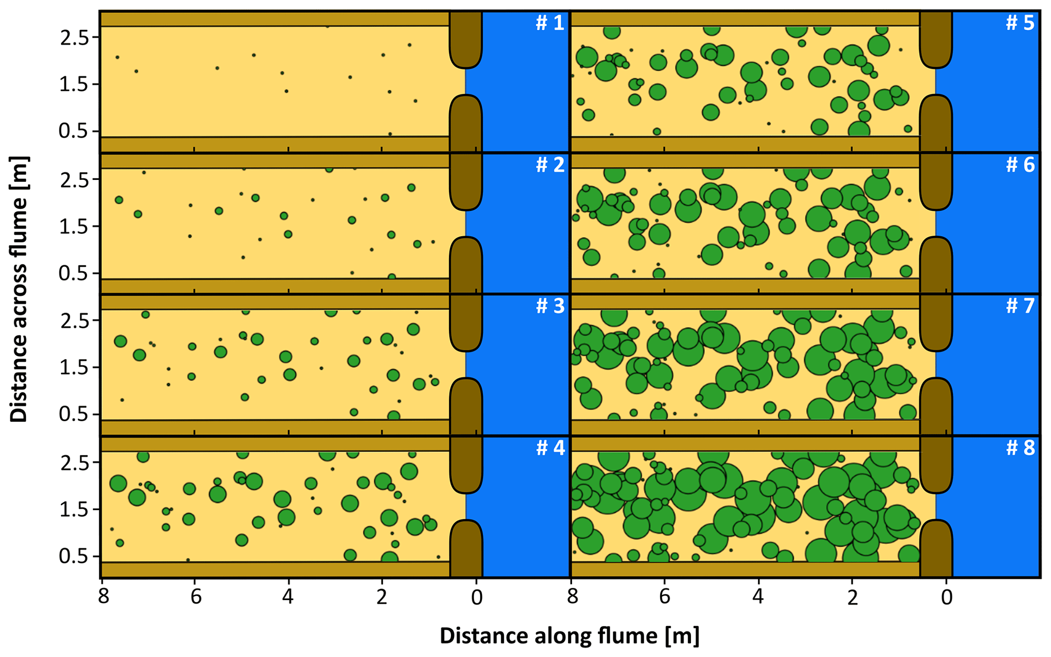
Figure 3Overview of the computer-generated, random patch locations over the course of eight sowing events in the patchy vegetation experiment. The green circles represent patches; 13 new patches appear per sowing event, while the existing patches expand. The numbers indicate the order of sowing events taking place with an interval of 500 tidal cycles in between: no. 1 represents the start of these events (after 1000 tidal cycles) and no. 8 the end (after 4500 tidal cycles).
2.3 Data collection and analysis
Digital elevation models were acquired using laser line scanning to analyse the morphological development of all experiments. Specifically, we worked with digital surface models (DSMs) as these include the top of the vegetation canopy. The laser line scanner was installed on a gantry above the flume, which moved over the entire length of the flume. It projected a laser line covering the complete width of the flume, which was then registered by a camera, within which the laser line position was identified and filtered at subpixel resolution. The laser line scanner had a horizontal resolution of about 0.75 mm and a vertical resolution of about 0.2 mm.
DSM acquisition requires a dry bed. Therefore, the flume was drained slowly to avoid morphological perturbation. DSMs were acquired every 440 or 500 tidal cycles (i.e. in line with the sowing events) until the end of every experiment. The first control experiment ended after 5000 tidal cycles when a morphodynamic equilibrium was reached (i.e. when the rate of change in system properties, such as eroded volume and channel migration, stabilized; Figs. 10, 11, and S6). In the hydrochorous experiment, another DSM was captured at 5500 tidal cycles. The patchy vegetation and second control experiment ran longer, until 10 000 tidal cycles, in order to check whether a morphodynamic equilibrium was indeed reached after 5000 tidal cycles. During the second half of these experiments, DSMs were acquired with an interval of 500 or 1000 cycles.
Additional to the laser line scanner, a single-lens reflex camera was mounted on the moving gantry. Overhead photos with a resolution of 4000 by 6000 pixels were taken from the dry and wet sand bed before and after DSMs were acquired. We took extra overhead photos during the vegetation experiments after the 4 d germination period following each sowing event. The images were calibrated for internal and external parameters (i.e. lens correction, geometric rectification) before they were stitched (see the Supplement and Leuven et al., 2018).
2.3.1 DSM processing
As mentioned before, DSMs were acquired from laser line scanning. First, the raw laser line scanner data underwent a calibration and correction process for the laser–camera system. Subsequently, the corrected data were filtered to exclude the 10th and 90th percentiles to remove outliers before interpolating them to a 3×3 mm grid size. Erosion and sedimentation maps were computed by subtracting a DSM with a DSM from the previous time step. During the hydrochorous vegetation experiment, an external disturbance slightly changed the position of the laser–camera system between 1500 and 3500 tidal cycles. Basic corrections were applied. Specifically, a correction value was retrieved by calculating the median of the differences between two DSMs (one “undisturbed” DSM and one DSM after the position of the laser–camera system changed). This value was then added to the elevation data.
2.3.2 Vegetation detection
The corrected and stitched overhead photos were used to detect vegetation and observe its cover development. We computed the green chromatic coordinate (GCC) as this colour index has been proven to track canopy development successfully (Nijland et al., 2014; Sonnentag et al., 2012). Furthermore, Sonnentag et al. (2012) have shown that GCC suppresses changes in scene illumination more effectively than other colour indices. The index was calculated using Eq. (1):
where B, R, and G represent the blue, red, and green bands from the images.
To explore the spatial variability in the temporal development of the vegetation cover as a function of distance from the tidal inlet, mean vegetation cover was computed over six zones of 1 m long along the full length of the tidal basin and across the complete width of the flume (3 m).
2.3.3 Channel geometric properties
Various channel geometric properties were quantified to compare the channel networks obtained by the different experiments. For this purpose, the Python toolbox TidalGeoPro (see Gourgue et al., 2022) was applied. This toolbox consists of a fully automated methodology to extract channel networks and their geometric properties from an input digital elevation model. The process involves several steps. First, a median neighbourhood analysis was performed on the DSMs (Liu et al., 2015). For each pixel, the median elevation was calculated among all neighbouring pixels within a window of several sizes to incorporate small-, medium-, and large-sized channels (i.e. 201 by 201, 501 by 501, and 1001 by 1001 pixels). If the difference between the window median and the local pixel elevation was below a certain threshold (0.0015, 0.005, and 0.0055 m) for at least one window size, the local pixel was identified as a channel. A raw channel network skeleton was retrieved containing some “erroneous” skeleton sections that did not connect to the channel network. This skeleton was cleaned in the next step by applying a threshold ratio (i.e. skeleton section length divided by the distance between the downstream node and the remaining skeleton). If a skeleton section length is below this threshold (1.7 in this case), it is removed. Then, a final channel network skeleton with equidistant skeleton points (3 mm) was computed as the centre line of the channel network. Finally, the tidal watershed area (based on distance to channel pixels) and the total upstream channel length (i.e. combined length of all channels with the tidal watershed) were computed for every skeleton point. The channel drainage density, the mean unchannelled path length, and the geometric efficiency were only computed at the inlet for the entire channel network.
The drainage density (D) represents the extent of tidal channelization and is defined as the total upstream channel length divided by the watershed surface area (Horton, 1932, 1945; Marani et al., 2003). However, it fails to capture the branching and meandering characteristics of the channel network (Kirchner, 1993; Marani et al., 2003). The geometric efficiency (eg) is a more appropriate measure to characterize these features (Kearney and Fagherazzi, 2016) and is defined as the inverse of drainage density (D−1) divided by the mean unchannelled path length (Marani et al., 2003). The mean unchannelled path length (mUPL) of a watershed is calculated as the mean distance to the closest channel, thus providing another proxy for the efficiency with which tidal channels drain a watershed (Marani et al., 2003; Tucker et al., 2001).
Finally, we computed a measure of local drainage densities (DL) for six zones (mentioned in Sect. 2.3.2) to explore spatial variability in drainage densities among zones at increasing distances from the tidal inlet. The local drainage density is the total channel length within the zone divided by the zone surface area.
2.3.4 Data correction for variability in initial system development
Although we aimed to start each of the four experiments from the same initial conditions, it is unavoidable to have slight differences in the initial sediment bed slopes and sediment properties. These differences induced different rates of channel development in the initial phases of the experiments when no vegetation was sown yet, which caused the channel development to occur faster or slower and hence to appear shifted in time when compared between the four experiments. To allow comparison of the later development of the four experiments, after the sowing of vegetation started and channel branching initialized, the origin of the time axis (i.e. number of tidal cycles) of each experiment was determined at a point in time where the same volume of sediment was displaced and the development decelerated. In this case, the erosion of the tidal basins in terms of volume per unit of time decelerated around the time an eroded volume of 0.02 m3 was reached (see Fig. S6). The curve, describing erosion volume with time, started to flatten at that point and the effects of the variability in initial system development damped out. Therefore, the timescale in the time series plots and maps was shifted up to about 1000–2000 cycles to a corrected tidal cycle number of zero when an eroded volume of 0.02 m3 was reached in every experiment.

Figure 4Plan view of digital surface models (DSMs) showing the four phases throughout the morphological development of the salt marsh experiments without vegetation but only sand (Control 1 and 2 in the two left columns), with hydrochorous seeding of vegetation and with patchy seeding (two right columns). Numbers indicate the corrected number of tidal cycles after which the DSM is shown.
3.1 Salt marsh development and dynamics
In general, four phases could be distinguished throughout the experiments' morphological development (Fig. 4). During the first phase, seen after around 500–1000 tidal cycles, one to three small channels formed around the inlet which expanded by backward erosion (see Fig. 5). In the next phase, around 1000–1500 tidal cycles (T=1.5 year to 2 years in real time), one of these channels developed into an elongated main channel with small side branches. The side branches were increasingly larger near the inlet, creating a Christmas-tree-shaped channel system. In the third phase, around 1500–2000 tidal cycles (–3 years), the main channel became wider and the channel system continued expanding through backward erosion during the ebb phases. During the flood phases, a sediment depositional lobe developed at the landward end of the channel system (see Figs. 4 and 5b, c). In the final phase, around 2000–2500 tidal cycles (–3.5 years), multiple channels branched off from the main channel in the landward part of the system. This led to an expansion of channels over the width of the flume and the development of channel bends cutting into the elevated borders. A dynamic channel bar pattern emerged between these channel bends cutting into the elevated borders. Past this point (>4000 tidal cycles − T≥5.5 years), morphological change declined drastically (see the Supplement – Figs. S1–S4) and a dynamic equilibrium was reached, in which channels were still able to migrate by erosion on one side and deposition on the other side of channels, but without much new channel expansion (Fig. 5d and e). The most landward area remained largely unaffected during the experiments.
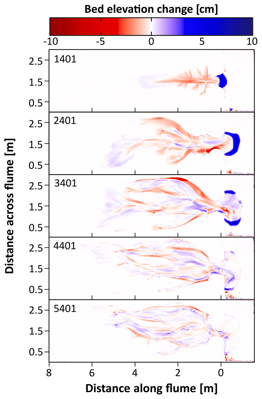
Figure 5Maps of erosion (red shades) and sedimentation (blue shades) resulting from the first control experiment for different time steps showing a decline in morphological change. Erosion and sedimentation are computed with respect to the previous time step in steps of 500 tidal cycles. For each time step, numbers indicate the corrected number of tidal cycles after which the erosion–sedimentation maps are shown. Only one experiment (Control 1) is shown here as an example. Erosion and sedimentation maps for the other experiments can be found in the Supplement.
Differences in morphological development between experiments started to occur once sufficient vegetation had been established, which was observed between phases three and four (Fig. 4). During both control experiments without vegetation, the main channel started to branch and widen close to the inlet, as the absence of vegetation enabled channel erosion. The main channel started to branch more landward in the vegetation experiments. Furthermore, in the vegetation experiments, a more landward elongated main channel developed, while the channel system widened further landward from the inlet. This pattern is most noticeable in the hydrochorous experiment, which could be caused by the establishment of vegetation fringing along the banks of the main channel. In the patchy experiment, an asymmetrical expansion of the channel system was observed as erosion of the left bank was limited by the presence of dense vegetation patches (Figs. 4, 7, and 8).
3.2 Vegetation establishment and disappearance
Analysis of the dynamic changes in vegetation cover depicted clear differences between the vegetation colonization patterns in the hydrochorous and patchy experiments (Fig. 7). In the hydrochorous experiment, vegetation first established along the channel banks close to the inlet. As the experiment progressed, vegetation settled more landward along the channel fringes (see Fig. 6b) and the depositional lobe. In the patchy experiment, the emergence of new and expansion of established circular patches can be seen. Patches disappeared partly or completely in unfavourable locations where channel erosion occurred or where the force of tidal flow was too strong. For instance, after 4500–5500 cycles, we observed that the left channel bend (assuming an observer looks from the seaward inlet into the landward direction ) was cutting through patches. Some of the uprooted vegetation was dispersed by the tide within the system and re-settled in different locations, such as the channel banks near the inlet. In both experiments, vegetation cover development started tentatively. Vegetation cover remained too low for visualization until 2500 tidal cycles, even though two sowing events had already occurred. Thereafter, vegetation cover started to increase. A similar vegetation cover development was observed in the most seaward zone of the tidal basin (Fig. 8a–c), followed by the zone with the lowest vegetation cover (Fig. 8d), coinciding with the development of channel bends. In the most landward part, an exponential increase in vegetation cover took place as disturbance by tidal flow or channel erosion remained low (Fig. 8e and f). Besides, uprooted and secondary dispersed vegetation tended to settle in these areas. Overall, vegetation mainly grew above mean sea level in the upper half of the intertidal zone (see Fig. S7).

Figure 6Photographs of vegetation-induced features in the experiments: (a) a germinating patch of seeds sown next to a channel, (b) a vegetated levee fringing along a channel, (c) channel initiation induced by vegetation, (d) channel bank stabilization by vegetation, and (e) sediment trapping induced by blocking of tidal flow in front of vegetation (flood flow direction indicated by arrow).
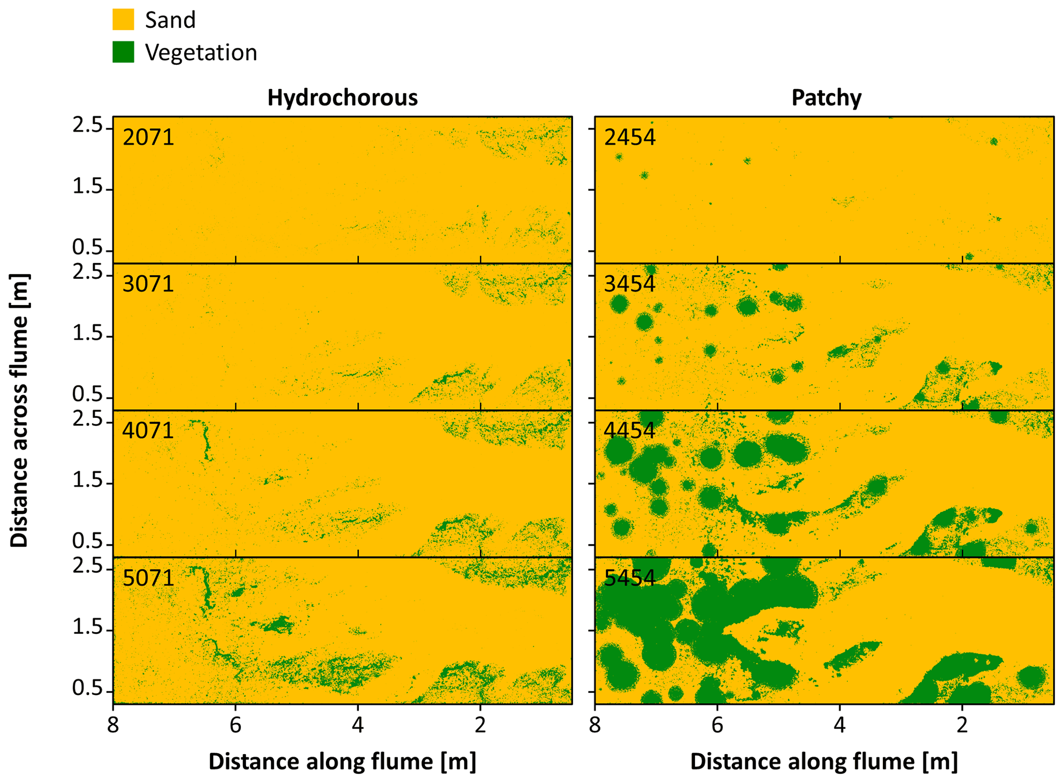
Figure 7Vegetation cover development in the hydrochorous and patchy seeding experiments. Numbers indicate the corrected number of tidal cycles after which the vegetation cover is shown.

Figure 8Development of vegetation cover over corrected number of tidal cycles in six zones divided along the length of the flume (i.e. at different distances from the tidal inlet): (a) 0–1 m, (b) 1–2 m, (c) 2–3 m, (d) 3–4 m, (e) 4–5 m, and (f) 5–6 m.
To get a better understanding of the vegetation cover development, a map of vegetation establishment and disappearance over time was made (Fig. 9). The hydrochorous experiment mainly showed disappearance of vegetation in the seaward part of the system. Specifically, the vegetated channel banks started eroding over time as the main channel widened (see Fig. 6d). In the patchy experiment disappearance mainly took place in the vegetated bar in the zone 3 to 4 m from the inlet during the intermediate stages. The uprooted vegetation of these patches then started to be redistributed and settle more landward, near other existing patches. The combination of this redistribution and settling of vegetation and continuously expanding patches around 5 to 6 m from the inlet resulted in a very dense patch of vegetation around 5500 tidal cycles (Figs. 8 and 9). During the second half of the patchy experiment (5000–10 000 tidal cycles − to 14 years in real time), the fixed vegetated bank around 1.5 to 3 m from the inlet eroded as the left channel bend (as seen from vertical top view) expanded laterally. The dense vegetation patch had a major impact on the system development as it limited the travel distance of tidal flow. Some vegetation closest to the landward channel ends got uprooted but remained in place as sand deposition restricted movement (see Fig. 6e). Shortly after 9000 tidal cycles, the right side of the vegetation patch breached, making space for system expansion. However, the uprooted vegetation (obtained from this breach) settled landward from the area, creating a new vegetation barrier.

Figure 9Maps showing the timing (expressed as corrected number of tidal cycles) of vegetation establishment and disappearance in the experiments with hydrochorous seeding (a) and patchy seeding (b). Green and blue colour shades depict vegetation establishment over time; green represents manual seeding and blue hydrochorous seed dispersal. Seeds were added until the corrected time step of ±5000 cycles. Red and yellow colour palettes depict disappearance over time; red corresponds to disappearance of manually sown patches and yellow to disappearance of hydrochorously spread vegetation. Hydrochorous seed dispersal in the patchy experiment is attributed to uprooted vegetation that dispersed with the flow and settled at different locations. Darker shades indicate vegetation establishment or disappearance during earlier stages of the experiments. Grey shows areas where vegetation never settled.
3.3 Channel geometric properties
The geometric properties of the developing channel systems were compared between all experiments after correcting the time axis and revealed certain differences. In the early stages of the experiments, from 0 to around 2000 tidal cycles, drainage density appeared to develop very similarly in all experiments but remained slightly smaller in the second control experiment (Fig. 10a). Around 2500 to 5000 tidal cycles, higher drainage densities were observed in the vegetation experiments. Differences became more quickly apparent in the hydrochorous experiment (2500 tidal cycles), while higher densities only started to become noticeable in the patchy experiment around 3500 tidal cycles. The higher degree of channelization is associated with vegetation establishment (Figs. 7–9). Drainage density stabilized after 5000 tidal cycles (corresponding to ±7 years in real time). Similar patterns were found in geometric efficiency (Fig. 10b) and mean unchannelled path length (Fig. 10c). However, it is apparent that mainly the hydrochorous experiment led to higher geometric efficiency around 3500 to 5000 tidal cycles, thus reflecting a more branching and meandering channel network. After 5000 tidal cycles, the patchy vegetation pattern also started to influence geometric efficiency. Geometric efficiency stabilized during the patchy and second control experiment during these final stages (>5000 tidal cycles). The mean unchannelled path lengths also began to differ between experiments around 2500 to 3000 tidal cycles. Once again, differences first started becoming visible in the hydrochorous experiment (around 2500 tidal cycles), while the patchy experiment lagged a bit behind (around 4500 tidal cycles). We observed larger mean unchannelled path lengths in both control experiments. A comparison between the vegetation experiments revealed larger mean unchannelled path lengths in the patchy experiment. Based on these results, it seems that the tidal channels of the hydrochorous experiment were most efficient in terms of draining a watershed.
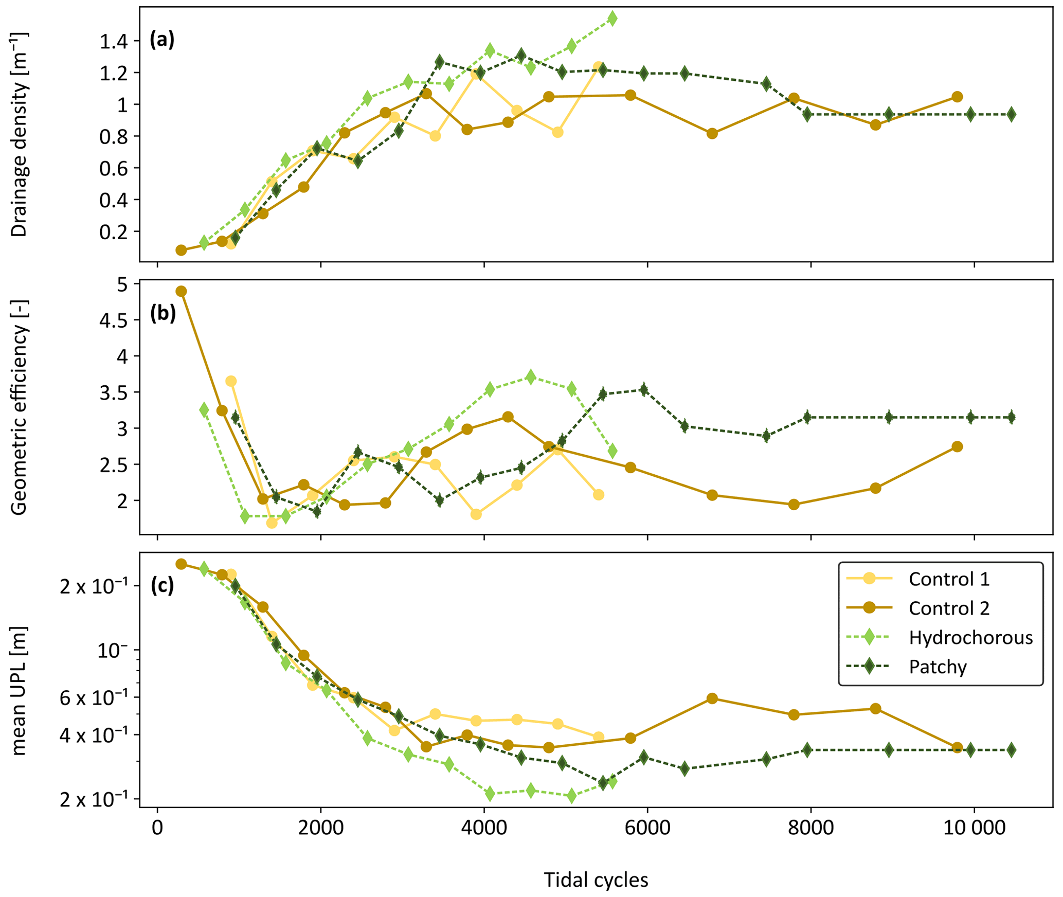
Figure 10Comparison of channel network metrics between the control experiments (yellow: Control 1; light brown: Control 2 and solid lines) and vegetated experiments (light green: hydrochorous; dark green: patchy and dashed lines). Evolution of (a) drainage density, (b) geometric efficiency, and (c) mean unchannelled path length (mean UPL) over time (expressed as corrected number of tidal cycles).
To have a closer look at spatial variability of the channel geometric properties within the simulated tidal basins, drainage densities were calculated for the aforementioned six zones (see Sect. 2.3.3). We observed a very dynamic pattern in the first two zones, starting from the inlet, without a discernible vegetation effect (Fig. 11a and b). Local drainage densities increased during the early stages of the experiments. Around 1500 to 2000 tidal cycles, a sudden decrease was noticed in all experiments. This decrease was caused by the widening of the main channel at the expense of side channels. The local drainage densities recovered from this decline as side channels reconnected and channel bends started moving more seaward. After 5000 tidal cycles, the variables stabilized.
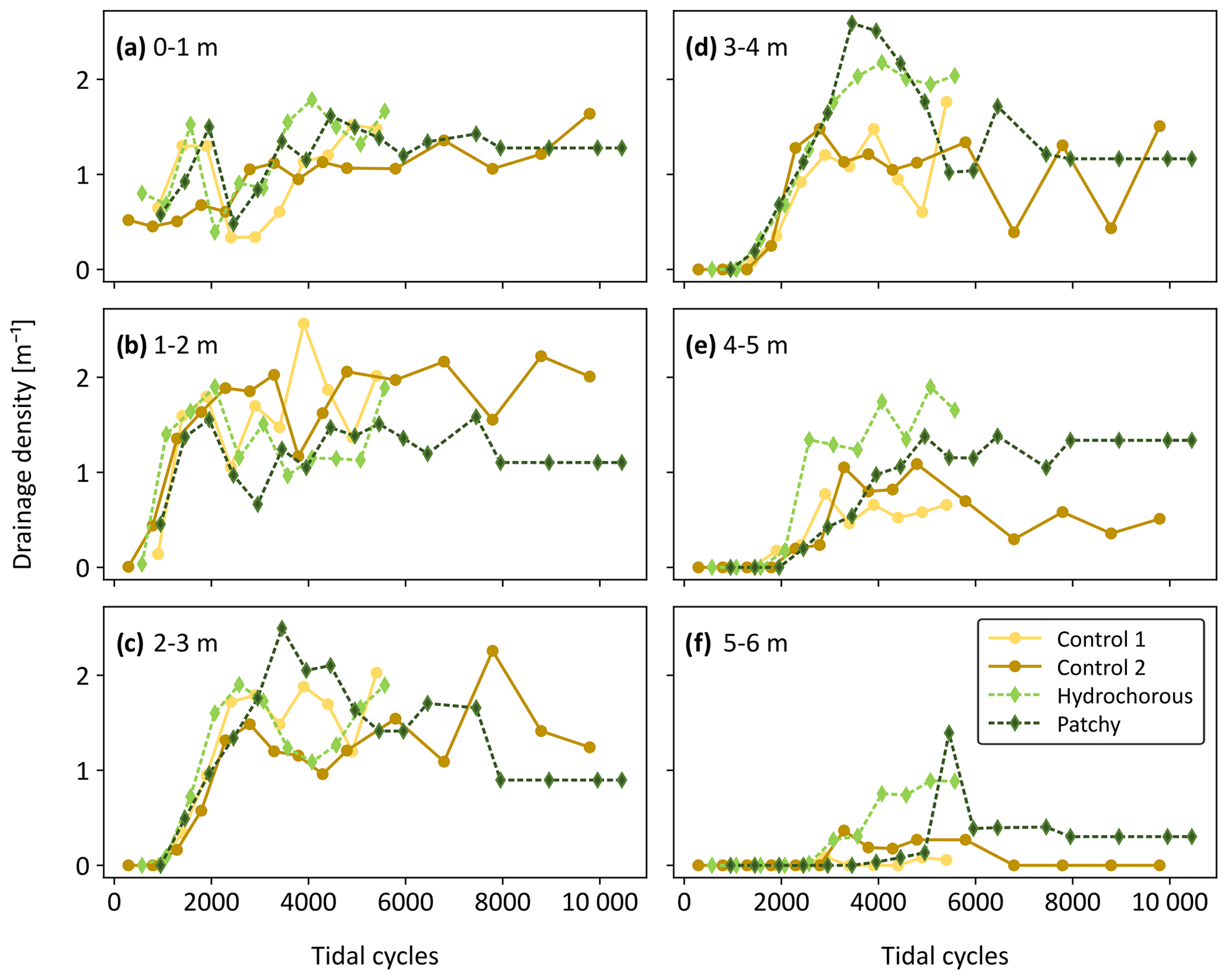
Figure 11Evolution of drainage density over time (expressed as corrected number of tidal cycles) in six zones divided along the length of the flume (i.e. at different distances from the tidal inlet): (a) 0–1 m, (b) 1–2 m, (c) 2–3 m, (d) 3–4 m, (e) 4–5 m, and (f) 5–6 m.
A similar trend was observed in the more landward zones (2 to 6 m – see Fig. 11c–e). Here, we finally started to see flow–vegetation interaction around 2500 tidal cycles. The patchy experiment reached peak local drainage density (DL) in zones 2 to 3 m and 3 to 4 m from the inlet, while the positive effect of vegetation on DL decreased in the most landward zones (4 to 5 m and 5 to 6 m from the inlet). The peak, seen around 5500 to 6000 tidal cycles, in the most landward zone coincided with a late expansion of central branching channels. Afterwards, the DL decreased since the left side branch became less active before reaching an equilibrium. In the hydrochorous experiment, peak drainage densities developed more landward. In contrast to the patchy experiment, the positive effect of vegetation on drainage density did not decrease but rather stabilized in the landward zones.
To get a better overview of where peak DL was reached, the variables were plotted along the length of the flume for specific time steps (Fig. 12). We focused on the time steps around 3000 to 5500 tidal cycles as by then sufficient vegetation had established to affect the system development. Earlier and later stages either did not include enough vegetation or exhibited stabilization in drainage densities. The location of local drainage density peaks differed between the unvegetated and vegetated experiments. The highest DL in both control experiments was found in the second closest zone to the inlet (Fig. 12b and c: 1 to 2 m), corresponding to the seaward system expansion seen in the morphological development (see Figs. S1–S4). Peak DL was reached more landward in the vegetation experiments. During the patchy experiment a peak was depicted around 2 to 3 m before reaching a plateau around 3 to 4 m, followed by a steep decrease in DL. A more diffused peak was observed in the hydrochorous experiment around 3 to 4 m before gradually decreasing in more landward zones. If we compare the drainage densities with the vegetation cover during the same time steps, we can notice that the variables mirror each other. Vegetation cover slowly increased in seaward areas before decreasing around 3 to 4 m. In landward areas, vegetation cover rose quickly over time, which is especially noticeable in the patchy experiment (Fig. 12e and f).

Figure 12Local drainage density and vegetation cover of all experiments between approximately 3000 and 5500 corrected tidal cycles for different zones along the length of the flume (i.e. at different distances from the tidal inlet). The solid lines represent peak drainage density.
Tidal channel networks and their geometric properties play an import role in the functioning of tidal wetlands (Fagherazzi et al., 1999; Friedrichs and Perry, 2001; Kearney and Fagherazzi, 2016; Temmerman et al., 2007). Novel scaled flume experiments, simulating a developing intertidal basin, were conducted to improve our understanding of the relative roles of abiotic and biotic processes in the development of tidal landscapes. The experiments showed that abiotic and biotic factors both affect the development and evolution of channel networks, where abiotic factors cause a general similarity in tidal system dimensions and development, but biotic factors cause considerable differences. The vegetated experiments led to more efficient channel networks, both on a local and system-wide scale. At the same time, the contrasting recruitment strategies produced surprising differences in channel geometric properties. The hydrochorous seeding experiment resulted in a better-drained system with a higher geometric efficiency compared to the patchy seeding experiment.
4.1 System-wide scale
Our findings on geometric channel network properties on a system-wide scale generally align with other studies showing more efficient channel networks in vegetated intertidal marshes compared to adjacent non-vegetated intertidal flats based on numerical models (e.g. Schwarz et al., 2014; Temmerman et al., 2007) and remote sensing analyses (e.g. Kearney and Fagherazzi, 2016; Vandenbruwaene et al., 2013). In line with these previous studies, we can explain this as vegetation establishment slowing down the flow inside vegetated zones while at the same time concentrating and accelerating the flow in between vegetated zones (Bouma et al., 2013; Vandenbruwaene et al., 2011), thereby favouring channel development and resulting in higher channel drainage density and efficiency. However, the differences we found between the two recruitment strategies are at first sight in contrast to the findings of Schwarz et al. (2018), who showed more efficient channel networks in systems with a slow, patchy plant colonization (by Spartina spp.) compared to systems with a fast, more homogenous plant colonization (by Salicornia spp.). The authors proposed that this can be related to local flow concentration. The resulting channel development is favoured between slowly colonizing vegetation patches, while such flow concentration is limited in the case of rapid, more homogeneous colonization. The different outcome of our experiments might be connected to the rate of vegetation cover development and final vegetation cover obtained. In the hydrochorous seeding experiment, the vegetation cover increased slowly over time and remained lower than in the patchy seeding experiment. Hence our hydrochorous experiment did not resemble a rapid, more homogeneous colonization pattern, as observed in marshes dominated by rapid and widespread hydrochorous seed dispersal by Salicornia spp. (Schwarz et al., 2018). Ultimately, in our hydrochorous experiment, the low vegetation cover and slow colonization might explain why flow concentration between the slowly developing vegetation zones favoured new channel development and why we saw more efficient channel networks than in the patchy experiment with more rapid colonization. As such, our experimental results suggest that the rate of vegetation cover development plays a more dominant role than vegetation patchiness in affecting the resulting channel network development. This finding is quite similar to previous non-tidal experimental results, suggesting that rapid vegetation colonization can inhibit channel network development (Piliouras et al., 2017; Tal and Paola, 2007), and it adds new insights compared to previous studies (Schwarz et al., 2018, 2022). An additional possibility is that the distribution of the circular patches in the patchy seeding experiment affected system development. Patches located in undisturbed areas (most landward from the inlet) could expand without inhibitions, while uprooted vegetation also tended to settle in these regions. This led to the growth of a giant patch on the landward side, which might have impeded system development and led to a lower channel network efficiency.
The observed differences between the vegetated and non-vegetated experiments (Figs. 10–12) were most noticeable during the transition from a bare to a “vegetated state” (tidal basin covered by a sufficient number of dense vegetation patches). Once a vegetated state was reached, channel geometric properties stabilized and differences between the experiments became less noticeable. The stabilization of network characteristics could be attributed to the stabilization of channel banks, slowing down of erosion, and potentially the slight reduction in tidal prism (e.g. Kleinhans et al., 2022; Marani et al., 2003; Tal and Paola, 2010; Vandenbruwaene et al., 2012, 2013; Weisscher et al., 2022). This stabilization or slight reduction in tidal prism might be related to the ebb delta, which kept growing in height and width over the course of the experiments and reduced the volume of water entering the system.

Figure 13Conceptual graph of main results. The effects of tidal prism (reflecting hydrodynamic energy) and vegetation cover on drainage density are expressed. The grey shaded regions represent zones varying in levels of tidal prism in which we see the highest drainage density for bare and vegetated landscapes. Bare landscapes show peak drainage density in regions with high tidal prism. Landscapes with hydrochorous and patchy recruitment strategies reach their peak in regions with intermediate hydrodynamic energy and vegetation cover. High vegetation cover in combination with low tidal prism leads to a decrease in drainage density.
4.2 Local scale
Based on the results on a local scale, we introduce a conceptual diagram (Fig. 13) proposing an interdependency between abiotic and biotic factors in the development of tidal channel networks. Abiotic processes (ambient hydrodynamic energy determined by tidal prism) control whether biotic factors (vegetation colonization) play an additional role in channel development. This seems consistent with the findings of the remote sensing analysis of Liu et al. (2022), where the authors suggest that abiotic factors have a stronger control on channel network geometry than biotic factors. The influence of biotic factors is secondary, but it remains important during system development (most notably during the early stages).
In the most seaward zones of the intertidal basin (Fig. 11; 0–3 m from the tidal inlet), we could not observe systematic differences in channel drainage density between the vegetated and non-vegetated experiments, suggesting that abiotic factors predominantly affect the formation of channels in this most seaward zone. We hypothesize that the tidal prism tends to be large there (leading to strong hydrodynamic energy) and impedes interaction between vegetation and channel development as vegetation establishment is hindered by the strong flow conditions, except for the edges of the tidal basin where lower-flow currents occur. Another possibility is that the existence of channels before sowing events commenced reduced the influence of plant–flow interactions (D'Alpaos et al., 2005; Schwarz et al., 2014).
In the more landward zone (Fig. 11; 3–5 m from the tidal inlet), where hydrodynamic energy is supposedly weaker due to a landward reduction in tidal prism, we observed higher channel drainage densities in the vegetated experiments than in the non-vegetated control experiments. This suggests that biotic factors play a dominant role during the development of channel networks in zones with more intermediate hydrodynamic energy levels. Plant–flow interactions can take place as vegetation is not washed away, while concentrated flow around vegetation patches promotes channel development, resulting in a higher degree of channelization (Schwarz et al., 2014; Temmerman et al., 2007; Vandenbruwaene et al., 2013, 2015). The more spatially homogeneous and hence weaker hydrodynamics in bare systems, on the other hand, may be responsible for the lower degree of channelization (e.g. Temmerman et al., 2005; Vandenbruwaene et al., 2013, 2015; Kearney and Fagherazzi, 2016). Field studies (such as Vandenbruwaene et al., 2015) have shown that this is related to more spatially homogenous sheet flow conditions on bare mudflats because of more spatially homogenous bed friction. In vegetated marshes, spatial heterogeneity in vegetation-induced friction promotes flow concentration towards bare channels.
Finally, in the most landward zones of the tidal basin (Fig. 11; 5–6 m from tidal inlet), we suggest that both biotic and abiotic factors no longer affect further channel network development. The hydrodynamic energy is too low to allow flow–topography feedback and plant–flow interactions. At the same time, dense vegetation patches impede system expansion by blocking the tidal flow, leading to low drainage densities.
Our findings might have important implications for understanding the relative role of abiotic and biotic processes in channel network development in tidal systems with an overall landward gradient of decreasing tidal hydrodynamic forces (e.g. back-barrier tidal basins with a seaward tidal inlet or tidal flat–marsh complexes with an overall seaward-sloping topography). Smaller-scale individual marsh islands with more complex topographies will likely show a more complex spatial pattern in tidal hydrodynamic forces than our experiments. Further research is required to investigate the interdependencies between these processes as it could provide valuable insights for managing, conserving, and restoring tidal marsh ecosystems. Besides, examining the influence of different hydrodynamic energy levels on the role of biotic processes in channel development could potentially help predict how tidal marshes may respond to environmental changes, including sea level rise or altered hydrological regimes. Overall, these findings highlight the complexity of tidal marsh ecosystem dynamics and emphasize the need for a holistic approach to managing and restoring tidal marshes.
Our findings uncovered an interdependency between abiotic and biotic processes in tidal channel network development in which the abiotic processes seem to control whether biotic processes affect channel development. The relative role of these processes relies on the different hydrodynamic energy zones found over the tidal landscape and the stage of the system development. Abiotic factors (flow–topography feedback) mainly dominate channel development in seaward zones with strong hydrodynamics as vegetation gets washed away. Biotic factors (i.e. vegetation colonization) start having an additional effect in more landward zones with an intermediate level of hydrodynamic energy as they allow plant–flow interaction. The vegetation patches lead to concentrated flow around vegetation patches, promoting channel development and a higher channel network efficiency. The resulting channel networks are mainly affected by the rate of vegetation cover development instead of vegetation patchiness. Once the hydrodynamic energy level gets too low, biotic processes hardly play a role. The tidal flow is too weak to ensure plant–flow interaction and initiate further channel network development. Both processes predominantly have an impact during the transition from a bare to a vegetated landscape.
DSMs and overhead imagery are available at https://doi.org/10.24416/UU01-0MNEHQ (Hautekiet et al., 2023).
The supplement related to this article is available online at: https://doi.org/10.5194/esurf-12-601-2024-supplement.
All authors conceptualized the study. SH and JER conducted the scaled experiments. SH and JER analysed the data with contributions from OG under the supervision of MGK and ST. SH wrote the draft of the paper, which was reviewed and edited by OG, MGK, and ST.
The contact author has declared that none of the authors has any competing interests.
Publisher's note: Copernicus Publications remains neutral with regard to jurisdictional claims made in the text, published maps, institutional affiliations, or any other geographical representation in this paper. While Copernicus Publications makes every effort to include appropriate place names, the final responsibility lies with the authors.
We would like to thank our BSc thesis and MSc thesis students Tim van Meurs and Thomas Veerman for the help provided during the scaled flume experiments. Furthermore, we cordially acknowledge the technical support of the experiments by the lab technicians and help during the sowing events. The resources and services used in part of the data analysis were provided by the VSC (Flemish Supercomputer Center), funded by the Research Foundation – Flanders (FWO) and the Flemish Government.
This research has been supported by the Fonds Wetenschappelijk Onderzoek (grant no. OZ8299).
This paper was edited by Andreas Lang and reviewed by Luca Carniello and three anonymous referees.
Allen, J.: Morphodynamics of Holocene salt marshes: a review sketch from the Atlantic and Southern North Sea coasts of Europe, Quaternary Sci. Rev., 19, 1155–1231, https://doi.org/10.1016/S0277-3791(99)00034-7, 2000.
Barbier, E. B., Hacker, S. D., Kennedy, C., Koch, E. W., Stier, A. C., and Silliman, B. R.: The value of estuarine and coastal ecosystem services, Ecol. Monogr., 81, 169–193, https://doi.org/10.1890/10-1510.1, 2011.
Bij de Vaate, I., Brückner, M. Z. M., Kleinhans, M. G., and Schwarz, C.: On the Impact of Salt Marsh Pioneer Species-Assemblages on the Emergence of Intertidal Channel Networks, Water Resour. Res., 56, e2019WR025942, https://doi.org/10.1029/2019WR025942, 2020.
Bouma, T. J., van Duren, L. A., Temmerman, S., Claverie, T., Blanco-Garcia, A., Ysebaert, T., and Herman, P. M. J.: Spatial flow and sedimentation patterns within patches of epibenthic structures: Combining field, flume and modelling experiments, Cont. Shelf Res., 27, 1020–1045, https://doi.org/10.1016/j.csr.2005.12.019, 2007.
Bouma, T. J., Temmerman, S., van Duren, L. A., Martini, E., Vandenbruwaene, W., Callaghan, D. P., Balke, T., Biermans, G., Klaassen, P. C., van Steeg, P., Dekker, F., van de Koppel, J., de Vries, M. B., and Herman, P. M. J.: Organism traits determine the strength of scale-dependent bio-geomorphic feedbacks: A flume study on three intertidal plant species, Geomorphology, 180–181, 57–65, https://doi.org/10.1016/j.geomorph.2012.09.005, 2013.
Byrne, R. J., Gammisch, R. A., and Thomas, G. R.: Tidal prism-inlet area relations for small tidal inlets, Int. Conf. Coast. Eng., 1, 149, https://doi.org/10.9753/icce.v17.149, 1980.
D'Alpaos, A., Fagherazzi, S., and Rinaldo, A.: Tidal network ontogeny: Channel initiation and early development, J. Geophys. Res., 110, F02001, https://doi.org/10.1029/2004JF000182, 2005.
D'Alpaos, A., Lanzoni, S., Mudd, S. M., and Fagherazzi, S.: Modeling the influence of hydroperiod and vegetation on the cross-sectional formation of tidal channels, Estuar. Coast. Shelf Sci., 69, 311–324, https://doi.org/10.1016/j.ecss.2006.05.002, 2006.
D'Alpaos, A., Lanzoni, S., Marani, M., and Rinaldo, A.: Landscape evolution in tidal embayments: Modeling the interplay of erosion, sedimentation, and vegetation dynamics, J. Geophys. Res., 112, F01008, https://doi.org/10.1029/2006JF000537, 2007.
D'Alpaos, A., Lanzoni, S., Marani, M., and Rinaldo, A.: On the tidal prism–channel area relations, J. Geophys. Res., 115, F01003, https://doi.org/10.1029/2008JF001243, 2010.
Davy, A. J., Bishop, G. F., and Costa, C. S. B.: Salicornia L. (Salicornia pusilla J. Woods, S. ramosissima J. Woods, S. europaea L., S. obscura P. W. Ball & Tutin, S. nitens P. W. Ball & Tutin, S. fragilis P. W. Ball & Tutin and S. dolichostachya Moss), J. Ecol., 89, 681–707, https://doi.org/10.1046/j.0022-0477.2001.00607.x, 2001.
Fagherazzi, S., Bortoluzzi, A., Dietrich, W. E., Adami, A., Lanzoni, S., Marani, M., and Rinaldo, A.: Tidal networks: 1. Automatic network extraction and preliminary scaling features from digital terrain maps, Water Resour. Res., 35, 3891–3904, https://doi.org/10.1029/1999WR900236, 1999.
Fagherazzi, S., Kirwan, M. L., Mudd, S. M., Guntenspergen, G. R., Temmerman, S., D'Alpaos, A., van de Koppel, J., Rybczyk, J. M., Reyes, E., Craft, C., and Clough, J.: Numerical models of salt marsh evolution: Ecological, geomorphic, and climatic factors, Rev. Geophys., 50, RG1002, https://doi.org/10.1029/2011RG000359, 2012.
Friedrichs, C. T. and Perry, J. E.: Tidal Salt Marsh Morphodynamics: A Synthesis, J. Coast. Res., 27, 7–37, 2001.
Geng, L., Gong, Z., Zhou, Z., Lanzoni, S., and D'Alpaos, A.: Assessing the relative contributions of the flood tide and the ebb tide to tidal channel network dynamics, Earth Surf. Proc. Land., 45, 237–250, https://doi.org/10.1002/esp.4727, 2020.
Gourgue, O., van Belzen, J., Schwarz, C., Vandenbruwaene, W., Vanlede, J., Belliard, J.-P., Fagherazzi, S., Bouma, T. J., van de Koppel, J., and Temmerman, S.: Biogeomorphic modeling to assess the resilience of tidal-marsh restoration to sea level rise and sediment supply, Earth Surf. Dynam., 10, 531–553, https://doi.org/10.5194/esurf-10-531-2022, 2022.
Gray, A. J.: Variation in Aster tripolium L., with particular reference to some British populations, PhD thesis, Keele University, https://eprints.keele.ac.uk/id/eprint/5892/ (last access: 2 December 2023), 1971.
Hautekiet, S., Rossius, J.-E., Gourgue, O., Kleinhans, M. G., and Temmerman, S.: Data supplement to `On the relative role of abiotic and biotic controls on channel network development: insights from scaled tidal flume experiments' (1.0), Utrecht University [data set], https://doi.org/10.24416/UU01-0MNEHQ, 2023.
Horton, R. E.: Drainage-basin characteristics, Trans. AGU, 13, 350, https://doi.org/10.1029/TR013i001p00350, 1932.
Horton, R. E.: Erosional development of streams and their drainage basins: hydrophysical approach to quantitative morphology. Bulletin of the Geological Society of America 56, 275–370, Prog. Phys. Geogr., 19, 533–554, https://doi.org/10.1177/030913339501900406, 1945.
Huiskes, A. H. L., Koutstaal, B. P., Herman, P. M. J., Beeftink, W. G., Markusse, M. M., and Munck, W. D.: Seed Dispersal of Halophytes in Tidal Salt Marshes, J. Ecol., 83, 559, https://doi.org/10.2307/2261624, 1995.
Jarrett, J. T.: Tidal Prism – Inlet Area Relationships, Coastal Engineering Research Center (US), General Investigation of Tidal Inlets Research Program Engineer Research and Development Center (US), https://hdl.handle.net/11681/3226 (last access: 3 September 2023), 1976.
Kearney, W. S. and Fagherazzi, S.: Salt marsh vegetation promotes efficient tidal channel networks, Nat. Commun., 7, 12287, https://doi.org/10.1038/ncomms12287, 2016.
Kirchner, J. W.: Statistical inevitability of Horton's laws and the apparent randomness of stream channel networks, Geology, 21, 591, https://doi.org/10.1130/0091-7613(1993)021<0591:SIOHSL>2.3.CO;2, 1993.
Kirwan, M. L. and Murray, A. B.: A coupled geomorphic and ecological model of tidal marsh evolution, P. Natl. Acad. Sci. USA, 104, 6118–6122, https://doi.org/10.1073/pnas.0700958104, 2007.
Kirwan, M. L., Murray, A. B., and Boyd, W. S.: Temporary vegetation disturbance as an explanation for permanent loss of tidal wetlands, Geophys. Res. Lett., 35, L05403, https://doi.org/10.1029/2007GL032681, 2008.
Kleinhans, M. G., Schuurman, F., Bakx, W., and Markies, H.: Meandering channel dynamics in highly cohesive sediment on an intertidal mud flat in the Westerschelde estuary, the Netherlands, Geomorphology, 105, 261–276, https://doi.org/10.1016/j.geomorph.2008.10.005, 2009.
Kleinhans, M. G., van der Vegt, M., van Scheltinga, R. T., Baar, A. W., and Markies, H.: Turning the tide: experimental creation of tidal channel networks and ebb deltas, Neth. J. Geosci., 91, 311–323, https://doi.org/10.1017/S0016774600000469, 2012.
Kleinhans, M. G., Braudrick, C., van Dijk, W. M., van de Lageweg, W. I., Teske, R., and van Oorschot, M.: Swiftness of biomorphodynamics in Lilliput- to Giant-sized rivers and deltas, Geomorphology, 244, 56–73, https://doi.org/10.1016/j.geomorph.2015.04.022, 2015a.
Kleinhans, M. G., van Scheltinga, R. T., van der Vegt, M., and Markies, H.: Turning the tide: Growth and dynamics of a tidal basin and inlet in experiments, J. Geophys. Res.-Earth, 120, 95–119, https://doi.org/10.1002/2014JF003127, 2015b.
Kleinhans, M. G., Leuven, J. R. F. W., Braat, L., and Baar, A.: Scour holes and ripples occur below the hydraulic smooth to rough transition of movable beds, Sedimentology, 64, 1381–1401, https://doi.org/10.1111/sed.12358, 2017a.
Kleinhans, M. G., van der Vegt, M., Leuven, J., Braat, L., Markies, H., Simmelink, A., Roosendaal, C., van Eijk, A., Vrijbergen, P., and van Maarseveen, M.: Turning the tide: comparison of tidal flow by periodic sea level fluctuation and by periodic bed tilting in scaled landscape experiments of estuaries, Earth Surf. Dynam., 5, 731–756, https://doi.org/10.5194/esurf-5-731-2017, 2017b.
Kleinhans, M. G., Roelofs, L., Weisscher, S. A. H., Lokhorst, I. R., and Braat, L.: Estuarine morphodynamics and development modified by floodplain formation, Earth Surf. Dynam., 10, 367—381, https://doi.org/10.5194/esurf-10-367-2022, 2022.
Krask, J. L., Buck, T. L., Dunn, R. P., and Smith, E. M.: Increasing tidal inundation corresponds to rising porewater nutrient concentrations in a southeastern U.S. salt marsh, PLoS ONE, 17, e0278215, https://doi.org/10.1371/journal.pone.0278215, 2022.
Leonardi, N., Carnacina, I., Donatelli, C., Ganju, N. K., Plater, A. J., Schuerch, M., and Temmerman, S.: Dynamic interactions between coastal storms and salt marshes: A review, Geomorphology, 301, 92–107, https://doi.org/10.1016/j.geomorph.2017.11.001, 2018.
Leuven, J. R. F. W., Braat, L., Dijk, W. M., Haas, T., Onselen, E. P., Ruessink, B. G., and Kleinhans, M. G.: Growing Forced Bars Determine Nonideal Estuary Planform, J. Geophys. Res.-Earth, 123, 2971–2992, https://doi.org/10.1029/2018JF004718, 2018.
Liu, Y., Zhou, M., Zhao, S., Zhan, W., Yang, K., and Li, M.: Automated extraction of tidal creeks from airborne laser altimetry data, J. Hydrol., 527, 1006–1020, https://doi.org/10.1016/j.jhydrol.2015.05.058, 2015.
Liu, Z., Gourgue, O., and Fagherazzi, S.: Biotic and abiotic factors control the geomorphic characteristics of channel networks in salt marshes, Limnol. Oceanogr., 67, 89–101, https://doi.org/10.1002/lno.11977, 2022.
Lokhorst, I. R., Lange, S. I., Buiten, G., Selaković, S., and Kleinhans, M. G.: Species selection and assessment of eco-engineering effects of seedlings for biogeomorphological landscape experiments, Earth Surf. Proc. Land., 44, 2922–2935, https://doi.org/10.1002/esp.4702, 2019.
Marani, M., Belluco, E., D'Alpaos, A., Defina, A., Lanzoni, S., and Rinaldo, A.: On the drainage density of tidal networks, Water Resour. Res., 39, 1040, https://doi.org/10.1029/2001WR001051, 2003.
Mariotti, G. and Fagherazzi, S.: Asymmetric fluxes of water and sediments in a mesotidal mudflat channel, Cont. Shelf Res., 31, 23–36, https://doi.org/10.1016/j.csr.2010.10.014, 2011.
Mcowen, C., Weatherdon, L., Bochove, J.-W., Sullivan, E., Blyth, S., Zockler, C., Stanwell-Smith, D., Kingston, N., Martin, C., Spalding, M., and Fletcher, S.: A global map of saltmarshes, Biodivers. Data J., 5, e11764, https://doi.org/10.3897/BDJ.5.e11764, 2017.
Meire, D. W. S. A., Kondziolka, J. M., and Nepf, H. M.: Interaction between neighboring vegetation patches: Impact on flow and deposition, Water Resour. Res., 50, 3809–3825, https://doi.org/10.1002/2013WR015070, 2014.
Myrick, R. M. and Leopold, L. B.: Hydraulic geometry of a small tidal estuary, US Geological Survey Professional Paper 422-B, US Geological Survey, 1–18, https://pubs.usgs.gov/publication/pp422B (last access: 25 June 2023), 1963.
Nijland, W., de Jong, R., de Jong, S. M., Wulder, M. A., Bater, C. W., and Coops, N. C.: Monitoring plant condition and phenology using infrared sensitive consumer grade digital cameras, Agr. Forest Meteorol., 184, 98–106, https://doi.org/10.1016/j.agrformet.2013.09.007, 2014.
Ortiz, A. C., Ashton, A., and Nepf, H.: Mean and turbulent velocity fields near rigid and flexible plants and the implications for deposition: Vegetation Impact On Flow And Deposition, J. Geophys. Res.-Earth, 118, 2585–2599, https://doi.org/10.1002/2013JF002858, 2013.
Piliouras, A. and Kim, W.: Delta size and plant patchiness as controls on channel network organization in experimental deltas, Earth Surf. Process. Land., 44, 259–272, https://doi.org/10.1002/esp.4492, 2019a.
Piliouras, A. and Kim, W.: Upstream and Downstream Boundary Conditions Control the Physical and Biological Development of River Deltas, Geophys. Res. Lett., 46, 11188–11196, https://doi.org/10.1029/2019GL084045, 2019b.
Piliouras, A., Kim, W., and Carlson, B.: Balancing Aggradation and Progradation on a Vegetated Delta: The Importance of Fluctuating Discharge in Depositional Systems, J. Geophys. Res.-Earth, 122, 1882–1900, https://doi.org/10.1002/2017JF004378, 2017.
Rinaldo, A., Fagherazzi, S., Lanzoni, S., Marani, M., and Dietrich, W. E.: Tidal networks: 2. Watershed delineation and comparative network morphology, Water Resour. Res., 35, 3905–3917, https://doi.org/10.1029/1999WR900237, 1999a.
Rinaldo, A., Fagherazzi, S., Lanzoni, S., Marani, M., and Dietrich, W. E.: Tidal networks: 3. Landscape-forming discharges and studies in empirical geomorphic relationships, Water Resour. Res., 35, 3919–3929, https://doi.org/10.1029/1999WR900238, 1999b.
Rogers, K., Kelleway, J. J., Saintilan, N., Megonigal, J. P., Adams, J. B., Holmquist, J. R., Lu, M., Schile-Beers, L., Zawadzki, A., Mazumder, D., and Woodroffe, C. D.: Wetland carbon storage controlled by millennial-scale variation in relative sea-level rise, Nature, 567, 91–95, https://doi.org/10.1038/s41586-019-0951-7, 2019.
Roner, M., D'Alpaos, A., Ghinassi, M., Marani, M., Silvestri, S., Franceschinis, E., and Realdon, N.: Spatial variation of salt-marsh organic and inorganic deposition and organic carbon accumulation: Inferences from the Venice lagoon, Italy, Adv. Water Resour., 93, 276–287, https://doi.org/10.1016/j.advwatres.2015.11.011, 2016.
Schwarz, C., Ye, Q. H., van der Wal, D., Zhang, L. Q., Bouma, T., Ysebaert, T., and Herman, P. M. J.: Impacts of salt marsh plants on tidal channel initiation and inheritance: salt marsh plants channel development, J. Geophys. Res.-Earth, 119, 385–400, https://doi.org/10.1002/2013JF002900, 2014.
Schwarz, C., Gourgue, O., van Belzen, J., Zhu, Z., Bouma, T. J., van de Koppel, J., Ruessink, G., Claude, N., and Temmerman, S.: Self-organization of a biogeomorphic landscape controlled by plant life-history traits, Nat. Geosci., 11, 672–677, https://doi.org/10.1038/s41561-018-0180-y, 2018.
Schwarz, C., van Rees, F., Xie, D., Kleinhans, M. G., and van Maanen, B.: Salt marshes create more extensive channel networks than mangroves, Nat. Commun., 13, 2017, https://doi.org/10.1038/s41467-022-29654-1, 2022.
Sonnentag, O., Hufkens, K., Teshera-Sterne, C., Young, A. M., Friedl, M., Braswell, B. H., Milliman, T., O'Keefe, J., and Richardson, A. D.: Digital repeat photography for phenological research in forest ecosystems, Agr. Forest Meteorol., 152, 159–177, https://doi.org/10.1016/j.agrformet.2011.09.009, 2012.
Stark, J., Plancke, Y., Ides, S., Meire, P., and Temmerman, S.: Coastal flood protection by a combined nature-based and engineering approach: Modeling the effects of marsh geometry and surrounding dikes, Estuar. Coast. Shelf Sci., 175, 34–45, https://doi.org/10.1016/j.ecss.2016.03.027, 2016.
Stark, J., Meire, P., and Temmerman, S.: Changing tidal hydrodynamics during different stages of eco-geomorphological development of a tidal marsh: A numerical modeling study, Estuar. Coast. Shelf Sci., 188, 56–68, https://doi.org/10.1016/j.ecss.2017.02.014, 2017.
Stefanon, L., Carniello, L., D'Alpaos, A., and Lanzoni, S.: Experimental analysis of tidal network growth and development, Cont. Shelf Res., 30, 950–962, https://doi.org/10.1016/j.csr.2009.08.018, 2010.
Tal, M. and Paola, C.: Dynamic single-thread channels maintained by the interaction of flow and vegetation, Geology, 35, 347, https://doi.org/10.1130/G23260A.1, 2007.
Tal, M. and Paola, C.: Effects of vegetation on channel morphodynamics: results and insights from laboratory experiments, Earth Surf. Proc. Land., 35, 1014–1028, https://doi.org/10.1002/esp.1908, 2010.
Tambroni, N., Bolla Pittaluga, M., and Seminara, G.: Laboratory observations of the morphodynamic evolution of tidal channels and tidal inlets: tidal channels and tidal inlets, J. Geophys. Res., 110, F04009, https://doi.org/10.1029/2004JF000243, 2005.
Temmerman, S., Bouma, T. J., Govers, G., Wang, Z. B., De Vries, M. B., and Herman, P. M. J.: Impact of vegetation on flow routing and sedimentation patterns: Three-dimensional modeling for a tidal marsh:, J. Geophys. Res., 110, F04019, https://doi.org/10.1029/2005JF000301, 2005.
Temmerman, S., Bouma, T. J., Van de Koppel, J., Van der Wal, D., De Vries, M. B., and Herman, P. M. J.: Vegetation causes channel erosion in a tidal landscape, Geology, 35, 631, https://doi.org/10.1130/G23502A.1, 2007.
Temmerman, S., De Vries, M. B., and Bouma, T. J.: Coastal marsh die-off and reduced attenuation of coastal floods: A model analysis, Global Planet. Change, 92–93, 267–274, https://doi.org/10.1016/j.gloplacha.2012.06.001, 2012.
Temmerman, S., Horstman, E. M., Krauss, K. W., Mullarney, J. C., Pelckmans, I., and Schoutens, K.: Marshes and Mangroves as Nature-Based Coastal Storm Buffers, Annu. Rev. Mar. Sci., 15, 95–118, https://doi.org/10.1146/annurev-marine-040422-092951, 2023.
Tucker, G. E., Catani, F., Rinaldo, A., and Bras, R. L.: Statistical analysis of drainage density from digital terrain data, Geomorphology, 36, 187–202, https://doi.org/10.1016/S0169-555X(00)00056-8, 2001.
Ursino, N., Silvestri, S., and Marani, M.: Subsurface flow and vegetation patterns in tidal environments, Water Resour. Res., 40, W05115, https://doi.org/10.1029/2003WR002702, 2004.
Vandenbruwaene, W., Temmerman, S., Bouma, T. J., Klaassen, P. C., de Vries, M. B., Callaghan, D. P., van Steeg, P., Dekker, F., van Duren, L. A., Martini, E., Balke, T., Biermans, G., Schoelynck, J., and Meire, P.: Flow interaction with dynamic vegetation patches: Implications for biogeomorphic evolution of a tidal landscape, J. Geophys. Res., 116, F01008, https://doi.org/10.1029/2010JF001788, 2011.
Vandenbruwaene, W., Meire, P., and Temmerman, S.: Formation and evolution of a tidal channel network within a constructed tidal marsh, Geomorphology, 151–152, 114–125, https://doi.org/10.1016/j.geomorph.2012.01.022, 2012.
Vandenbruwaene, W., Bouma, T. J., Meire, P., and Temmerman, S.: Bio-geomorphic effects on tidal channel evolution: impact of vegetation establishment and tidal prism change, Earth Surf. Proc. Land., 38, 122–132, https://doi.org/10.1002/esp.3265, 2013.
Vandenbruwaene, W., Schwarz, C., Bouma, T. J., Meire, P., and Temmerman, S.: Landscape-scale flow patterns over a vegetated tidal marsh and an unvegetated tidal flat: Implications for the landform properties of the intertidal floodplain, Geomorphology, 231, 40–52, https://doi.org/10.1016/j.geomorph.2014.11.020, 2015.
van Dobben, H. F., de Groot, A. V., and Bakker, J. P.: Salt Marsh Accretion With and Without Deep Soil Subsidence as a Proxy for Sea-Level Rise, Estuar. Coasts, 45, 1562–1582, https://doi.org/10.1007/s12237-021-01034-w, 2022.
Van Putte, N., Temmerman, S., Verreydt, G., Seuntjens, P., Maris, T., Heyndrickx, M., Boone, M., Joris, I., and Meire, P.: Groundwater dynamics in a restored tidal marsh are limited by historical soil compaction, Estuar. Coast. Shelf Sci., 244, 106101, https://doi.org/10.1016/j.ecss.2019.02.006, 2020.
Vlaswinkel, B. M. and Cantelli, A.: Geometric characteristics and evolution of a tidal channel network in experimental setting, Earth Surf. Proc. Land., 36, 739–752, https://doi.org/10.1002/esp.2099, 2011.
Weisscher, S. A. H., Van den Hoven, K., Pierik, H. J., and Kleinhans, M. G.: Building and Raising Land: Mud and Vegetation Effects in Infilling Estuaries, J. Geophys. Res.-Earth, 127, e2021JF006298, https://doi.org/10.1029/2021JF006298, 2022.
Xin, P., Wilson, A., Shen, C., Ge, Z., Moffett, K. B., Santos, I. R., Chen, X., Xu, X., Yau, Y. Y. Y., Moore, W., Li, L., and Barry, D. A.: Surface Water and Groundwater Interactions in Salt Marshes and Their Impact on Plant Ecology and Coastal Biogeochemistry, Rev. Geophys., 60, e2021RG000740, https://doi.org/10.1029/2021RG000740, 2022.
Zhou, Z., Olabarrieta, M., Stefanon, L., D'Alpaos, A., Carniello, L., and Coco, G.: A comparative study of physical and numerical modeling of tidal network ontogeny, J. Geophys. Res.-Earth, 119, 892–912, https://doi.org/10.1002/2014JF003092, 2014.
Zong, L. and Nepf, H.: Flow and deposition in and around a finite patch of vegetation, Geomorphology, 116, 363–372, https://doi.org/10.1016/j.geomorph.2009.11.020, 2010.
Zong, L. and Nepf, H.: Spatial distribution of deposition within a patch of vegetation, Water Resour. Res., 47, 2010WR009516, https://doi.org/10.1029/2010WR009516, 2011.
Zong, L. and Nepf, H.: Vortex development behind a finite porous obstruction in a channel, J. Fluid Mech., 691, 368–391, https://doi.org/10.1017/jfm.2011.479, 2012.