Evaluating the accuracy of binary classifiers for geomorphic applications

Increased access to high-resolution topography has revolutionized our ability to map out fine-scale topographic features at watershed to landscape scales. As our “vision” of the land surface has improved, so has the need for more robust quantification of the accuracy of the geomorphic maps we derive from these data. One broad class of mapping challenges is that of binary classification whereby remote sensing data are used to identify the presence or absence of a given feature. Fortunately, there is a large suite of metrics developed in the data sciences well suited to quantifying the pixel-level accuracy of binary classifiers. This analysis focuses on how these metrics perform when there is a need to quantify how the number and extent of landforms are expected to vary as a function of the environmental forcing (e.g., due to climate, ecology, material property, erosion rate). Results from a suite of synthetic surfaces show how the most widely used pixel-level accuracy metric, the F₁ score, is particularly poorly suited to quantifying accuracy for this kind of application. Well-known biases to imbalanced data are exacerbated by methodological strategies that calibrate and validate classifiers across settings where feature abundances vary. The Matthews correlation coefficient largely removes this bias over a wide range of feature abundances such that the sensitivity of accuracy scores to geomorphic setting instead embeds information about the size and shape of features and the type of error. If error is random, the Matthews correlation coefficient is insensitive to feature size and shape, though preferential modification of the dominant class can limit the domain over which scores can be compared. If the error is systematic (e.g., due to co-registration error between remote sensing datasets), this metric shows strong sensitivity to feature size and shape such that smaller features with more complex boundaries induce more classification error. Future studies should build on this analysis by interrogating how pixel-level accuracy metrics respond to different kinds of feature distributions indicative of different types of surface processes.

1 Motivation

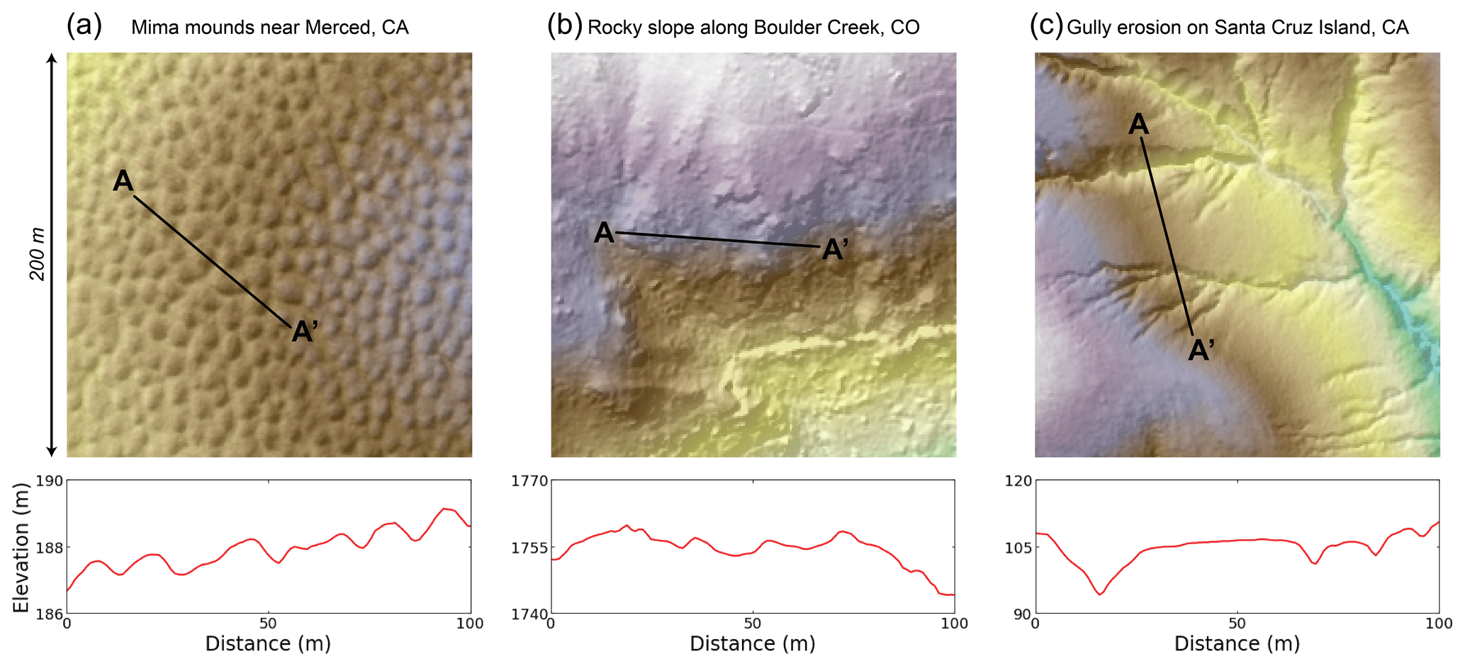
Figure 1 (a) Mima mounds near Merced, CA, USA; (b) bedrock outcrops along Boulder Creek, CO, USA; and (c) gully erosion on Santa Cruz Island, CA, USA, as observed from 1 m shaded relief maps. Note that even though the areal extent is the same among these scenes (200 × 200 m), topographic relief is drastically different (total relief in a is 7 m, in b is 146 m, and in c is 76 m). The 100 m elevation transects from A to A' for each site are shown to illustrate how different features manifest as roughness elements in the topography. Airborne lidar for the Mima mounds and rocky slope sites was flown by the National Center for Airborne Laser Mapping (NCALM). Airborne lidar for the gully erosion site was flown by the United States Geological Survey (USGS). All lidar datasets were downloaded from OpenTopography (Reed, 2006; Anderson et al., 2012; 2010 Channel Islands Lidar Collection, 2012). Interpretations of features classified from lidar data can be found in Reed and Amundson (2012), Rossi et al. (2020), and Korzeniowska et al. (2018) for the Mima mound, rocky slope, and gully sites, respectively.

High-resolution topographic datasets are transforming our ability to characterize the fine-scale structure of the Earth's surface (Passalacqua et al., 2015). Airborne lidar, in particular, has changed how geomorphic fieldwork is conducted by enabling scientists to quantify the form and extent of meter-scale features over large areas (Roering et al., 2013). Because lidar “sees” through vegetation, lidar has accelerated progress in both discovery science and testing hypotheses wherein the prevalence of features is expected to vary as a function of the environmental forcing (e.g., in response to differences in climate, ecology, material property, erosion rate). Airborne lidar has now been used to map Mima mounds (Reed and Amundson, 2012), termite mounds (Levick et al., 2010; Davies et al., 2014), tree throw pits and mounds (Roering et al., 2010; Doane et al., 2023), landslide boundaries and classes (Jaboyedoff et al., 2012; Bunn et al., 2019; Prakesh et al., 2020), channel networks (Pirotti and Tarolli, 2010; Clubb et al., 2014; Korzeniowska et al., 2018), bedrock structure (Cunningham et al., 2006; Pavlis and Bruhn, 2011; Morell et al., 2017), and bedrock exposure (DiBiase et al., 2012; Milodowski et al., 2015; Rossi et al., 2020).

Figure 1 shows three examples of features that can be mapped using 1 m airborne lidar data. The utility of the binary classification of feature locations for each of these geomorphic applications is clear. However, examples also highlight how the number, size, shape, amplitude, and pattern of features can vary. Regular, repeating morphologies with a characteristic spatial scale (e.g., Mima mounds in Fig. 1a; Reed and Amundson, 2012) pose different challenges to classification than irregular, heterogeneous morphologies that occur at many scales (e.g., bedrock exposure in Fig. 1b; Rossi et al., 2020). Furthermore, the importance of flowing water for surface processes means that many geomorphic features form directional networks with substantial anisotropy (e.g., gully erosion in Fig. 1c; Korzeniowska et al., 2018). Perhaps unsurprisingly then, accuracy assessment in the geomorphic literature has varied a lot even as formal methods for evaluating pixel-level accuracy of binary classifiers are now becoming standard practice in the remote sensing and machine learning literature (e.g., Wang et al., 2019; Prakesh et al., 2020; Agren et al., 2021). Slow adoption of these standard methods in accuracy assessment may arise from two tendencies of geomorphic studies that employ lidar classifiers: (1) process-based studies are typically more interested in the properties and densities of features rather than their contingent locations, and (2) classifiers are expected to work across large gradients in the prevalence of features to test our understanding of the relevant transport laws at play. The former tendency arises from the fact that predicting the actual locations of features (e.g., mounds, outcrops, channels) is not usually a viable target for numerical models of landscapes where uncertainty in initial conditions and the stochastic nature of processes preclude a deterministic forecasting of the precise locations of features (e.g., Barnhart et al., 2020). The latter tendency arises from the need to use classified data to constrain natural experiments wherein geomorphic transport laws (Dietrich et al., 2003) can be tested against governing variables (e.g., across climo-, eco-, litho-, or tectono-sequences). As shown below, these tendencies can be at odds with pixel-level accuracy metrics designed to assess positional accuracy for balanced data (i.e., data for which the frequency of positive and negative values are similar).

Nevertheless, there are several important benefits to adopting pixel-level accuracy metrics when reporting the success of geomorphic classifiers. First, these metrics provide common standards for evaluating classifier accuracy across studies, including direct comparison between proxy-based classifiers and those developed using machine learning. Second, trends in pixel-level accuracy scores may reveal patterns in the spatial structure of error. Third, pixel-level measures are easy to apply to new objectives as long as their limitations are properly considered. This paper focuses on how two widely used metrics, F measures (van Rijsbergen, 1974; Chinchor, 1992) and the Matthews correlation coefficient (Matthews, 1975; Baldi et al., 2000), perform when the research design intentionally calibrates and tests binary classifiers across large gradients in how balanced the data are. The general approach is to synthetically generate “model” and “truth” data that have a known error structure. Pixel-level accuracy scores are then calculated as a function of feature abundance. Despite the simplicity of the scenarios considered, this analysis helps constrain the range over which pixel-level metrics can be reliably compared across gradients in feature abundance. Synthetic scenarios also reveal how the shape and scale of individual objects can strongly influence pixel-level scores when there are small co-registration errors between model and truth data.

2 Approach

One common use of binary classifiers is to build an inventory of feature boundaries and abundances using remotely sensed data. This typically entails using scenes where the truth is known through detailed field or air photo mapping. An algorithm built from an independent data source (e.g., lidar) is then used to model the locations of features. Models are commonly trained and tested so that the classifier can be used for larger-scale geomorphic mapping. If the density, size distribution, and form of features vary from scene to scene, then it is important to understand how pixel-level accuracy metrics will perform as a function of scene-level properties (e.g., feature fraction). To mimic this task, this paper examines how two widely used accuracy metrics, the F₁ score and Matthews correlation coefficient (MCC), behave on synthetic truth and model data. Synthetic truth data are generated by randomly placing features in a scene at a given abundance. Model data are either independent from truth data or derived from the truth data using an assumed error structure. Pixel-level accuracy scores are then calculated for each scene.

2.1 Grid generation

To generate grids of features within a matrix, the pseudo-random number generator in NumPy is used to create a scene of size m×n cells. Continuous values are converted into binary classes (0: matrix; 1: feature) based on a user-specified value for the feature fraction (f_f), which is simply the fraction of the surface covered by features. The simplest scenario is for features with a size of 1 pixel. While synthetic surfaces are scale-free, results are reported assuming a grid spacing of 1 m to represent a typical case using airborne lidar. To simulate features that have a scale greater than 1 m², the pseudo-random numbers instead specify a first guess at the locations of the centers of incipient features. The first guess at the number of features is calculated by finding the integer number of features of length l that most closely matches f_f. However, as the number of feature centers increases, so does the probability that two neighboring objects overlap and coalesce into a larger object. As such, the first guess generally produces an actual feature fraction lower than the user-specified value. The ratio between the specified f_f and this underestimate is then used to proportionally increase the number of incipient features in the model domain. The process is iterated until either the synthetic fraction is within 0.5 % of the specified value or 50 iterations, whichever comes first. The number of incipient objects is always higher than the actual number of objects in the scene because smaller incipient features increasingly coalesce into larger objects at higher feature fractions.

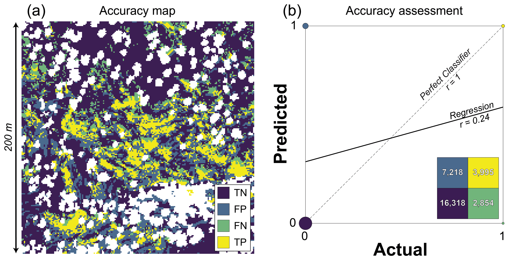
Figure 2 (a) Pixel classes for Fig. 1b and (b) the corresponding confusion matrix (inset) and correlation plot (main). In (a), the four outcomes of the binary classification are shown in color (TN: true negative; FP: false positive; FN: false negative; TP: true positive). The areas in white were obscured by the vegetation canopy in air photos (24 % of area) and thus excluded from accuracy assessment. In (b), the colors of each cell in the confusion matrix and each point in the plot are the same as in (a). The number of observations for each class is shown in the confusion matrix, and point sizes on the plot are scaled to the relative frequency of each value. This classified map is site P01 from Rossi et al. (2020), where more details on mapping methods are described.

Table 1 Accuracy metrics for Fig. 2 using the alternative target classes of bedrock and soil.

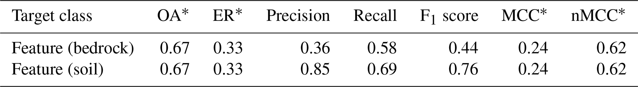
^* Metrics that do not vary as a function of the target class in binary classification.

All scenarios in this study rely on comparing simulated truth and model grids across the full range of feature fractions (0 < f_f < 1). Where the truth and model data are independent of each other, the two grids are generated using different pseudo-random seed numbers in NumPy (Sect. 3). In scenarios in which the model grid is dependent on the truth grid, the model grid is a copy of the truth data using the specified error structure. Details for how random error (Sect. 4.1), systematic error (Sect. 4.2), and random plus systematic error (Sect. 4.3) are implemented are described in context below. For each scenario, the truth and model grids are evaluated by building the confusion matrix and calculating accuracy metrics at each feature fraction (Sect. 2.2).

2.2 Pixel-level accuracy metrics

While there are many metrics used to quantify the accuracy of binary classifiers, the focus of this paper is on two of the most widely used ones: the F₁ score and Matthews correlation coefficient (MCC). These metrics are frequently used to evaluate pixel-level performance of classified maps generated from machine learning (e.g., Wang et al., 2019; Prakesh et al., 2020; Agren et al., 2021). Application of these metrics need not be limited to the training and testing of machine learning algorithms. They are broadly useful to any binary classification task for which positional accuracy is important. Both the F₁ score and MCC can be calculated directly from the confusion matrix. The confusion matrix for binary classification is a 2×2 table where the column headers are the true classes and the row headers are the model classes, thereby summarizing the occurrence of the four possible classification outcomes: true negatives (TNs), true positives (TPs), false positives (FPs), and false negatives (FNs).

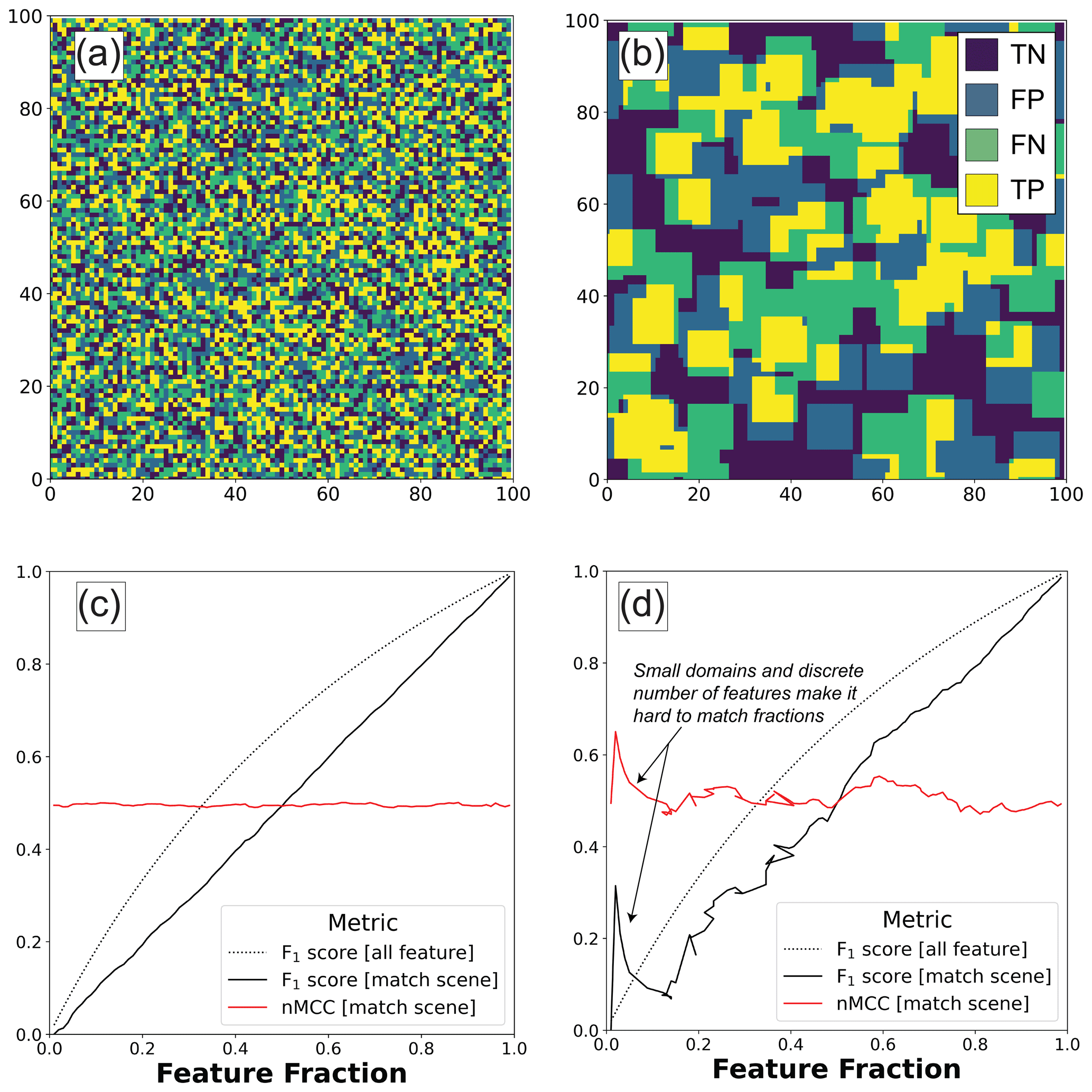
Figure 3 Classified 100×100 m maps of (a) 1 m and (b) 10 m long incipient features showing the four classification outcomes (TN: true negative, FN: false negative, FP: false positive, TP: true positive). How accuracy scores vary as a function of feature fraction is also shown for (c) 1 m and (d) 10 m long incipient features. The “all feature” scenario is where the model assumes that the entire surface is a feature with no matrix, regardless of scene-level properties. The “match scene” scenario is where the model data match the actual feature fraction, but whose feature locations are independent of each other. In (a–b), example maps are shown for the case in which 50 % of the surface is covered by features. In (c–d), the normalized Matthews correlation coefficient (nMCC) is only shown for the match scene scenario because it is undefined in the “all feature” scenario.

For example, the scene in Fig. 1b is readily reclassified into these four outcomes (Fig. 2a) using the feature mapping from Rossi et al. (2020). The frequency of these outcomes is summarized using the confusion matrix (Fig. 2b inset). The simplest accuracy metric is the overall accuracy (OA) and its complement the error rate (ER), where

$$\begin{array}{}\text{(1)}& {\displaystyle }\mathrm{OA}={\displaystyle \frac{\mathrm{TP}+\mathrm{TN}}{\mathrm{TP}+\mathrm{TN}+\mathrm{FP}+\mathrm{FN}}},\text{(2)}& {\displaystyle }\mathrm{ER}={\displaystyle \frac{\mathrm{FP}+\mathrm{FN}}{\mathrm{TP}+\mathrm{TN}+\mathrm{FP}+\mathrm{FN}}}.\end{array}$$

While OA and ER are straightforward to calculate, they provide little insight into the relative frequencies of FP and FN. To address this limitation, there is a large family of accuracy metrics that better characterize different types of error. For example, precision and recall explicitly characterize the relative frequencies of FP and FN. Precision, also known as the positive predictive value, is the ratio of true positives to all positives predicted by the model (accounts for FP):

$$\begin{array}{}\text{(3)}& \mathrm{Precision}={\displaystyle \frac{\mathrm{TP}}{\mathrm{TP}+\mathrm{FP}}}.\end{array}$$

Recall, also known as the true positive rate, is the ratio of true positives to all positives (accounts for FN):

$$\begin{array}{}\text{(4)}& \mathrm{Recall}={\displaystyle \frac{\mathrm{TP}}{\mathrm{TP}+\mathrm{FN}}}.\end{array}$$

Figure 2 is an example in which the precision is low (0.36), but the recall is reasonably good (0.58) (Table 1). F measures were designed to summarize precision and recall into a single metric (van Rijsbergen, 1974; Chinchor, 1992). The case in which both are equally weighted is referred to as the F₁ score, where

$$\begin{array}{}\text{(5)}& {\mathrm{F}}_{\mathrm{1}}\mathrm{score}={\displaystyle \frac{\mathrm{2}\times \mathrm{TP}}{\left(\mathrm{2}\times \mathrm{TP}\right)+\mathrm{FP}+\mathrm{FN}}}.\end{array}$$

By representing the harmonic mean of precision and recall, this metric accounts for both errors of omission and commission. F₁ scores only characterize the success at identifying the target class, and low values can occur even if the overall accuracy is high because it excludes true negatives. As such, this metric is sensitive to the prevalence of positive values. Higher F₁ scores are favored when the positive class is more abundant (e.g., Chicco and Jurman, 2020). Related to this sensitivity to imbalanced data is the property of asymmetry. Asymmetric metrics are those for which the accuracy score differs when the target classes are switched. Table 1 shows that the F₁ score for Fig. 2 would be 72 % higher if the target feature was soil instead of bedrock. Asymmetry arises because there is more soil than bedrock in the scene and TNs are not included in calculations of precision, recall, or F₁ score. These well-known limitations of F measures are better handled by metrics that incorporate all four classes of the confusion matrix. One such metric is the Matthews correlation coefficient (MCC), where

$$\begin{array}{}\text{(6)}& \begin{array}{rl}& \mathrm{MCC}=\\ & {\displaystyle \frac{\left(\mathrm{TP}\times \mathrm{TN}\right)-\left(\mathrm{FP}\times \mathrm{FN}\right)}{\sqrt{\left(\mathrm{TP}+\mathrm{FP}\right)\times \left(\mathrm{TP}+\mathrm{FN}\right)\times \left(\mathrm{TN}+\mathrm{FP}\right)\times \left(\mathrm{TN}+\mathrm{FN}\right)}}}.\end{array}\end{array}$$

MCC is equivalent to a Pearson correlation coefficient where the model classes are regressed against the true classes in a binary classification task (Fig. 2b). Values of MCC can be similarly interpreted where −1.0 indicates perfect anticorrelation, 0 indicates no correlation, and 1.0 indicates perfect correlation. And while MCC is just one of several metrics that include all four quadrants of the confusion matrix (e.g., balanced accuracy, markedness, Cohen's kappa), recent work suggests that MCC is the most robust to imbalanced data (Chicco and Jurman, 2020; Chicco et al., 2021a, b). In this analysis, I report a normalized version of MCC as

$$\begin{array}{}\text{(7)}& \mathrm{nMCC}={\displaystyle \frac{\mathrm{MCC}+\mathrm{1}}{\mathrm{2}}}.\end{array}$$

By rescaling MCC from zero to 1, nMCC facilitates comparison with the F₁ score on plots and in discussion. It is worth noting that interpretations of low values of nMCC differ from interpretations of low values of the F₁ score. The former implies anticorrelation between model and truth data, while the latter does not. For example, the scene in Fig. 2 indicates a weak positive correlation (i.e., nMCC greater than 0.5) even though the F₁ score is lower than 0.5 (Table 1). As such, direct comparison of these metrics should be done with caution.

3 Independence between truth and model data

The distinction between pixel-level and scene-level accuracy, in part, motivates the approach taken to examine how accuracy metrics handle imbalanced data in this study. Pixel-level accuracy requires that the precise locations of features are honored, with a lower bound to feature detection set by the spatial resolution of the data used. Scene-level accuracy characterizes the mismatch between model and truth data at some coarser scale and typically assesses statistical properties of the target feature class (e.g., bedrock fraction, mound densities, drainage densities). While high pixel-level accuracy ensures high scene-level accuracy, the converse need not be true. Given the importance of developing binary classifiers that work across a range of feature densities and sizes, there is a need to better understand how pixel-level accuracy metrics perform across a range of scene-level properties like feature fraction. One mark of a good accuracy metric is its ability to diagnose the case of independence. In this context, independence means that the locations of features in the model contain no information about the true locations of features. If accuracy metrics produce similar scores when the model and truth data are independent from each other, then it means the metric can be reliably compared for different feature fractions. A perhaps trivial example is the case in which feature fractions are assumed to be constant (e.g., total feature coverage) regardless of the true feature fraction. A more interesting example is the case in which scene-level fractions are the same in the truth and model data (i.e., high scene-level accuracy) but the actual locations of features are unrelated (i.e., low pixel-level accuracy).

Figure 3 shows the sensitivity of the F₁ score and nMCC to imbalanced data when the model and truth data are independent from each other ($m=n=$ 100). Each scenario assumes features are randomly distributed throughout the scene for any given feature fraction. In the first scenario, the classifier predicts that the feature is found everywhere regardless of the truth data (dashed lines). Because this “all feature” model produces neither false negatives nor true negatives, nMCC is undefined in this scenario (see Eqs. 6–7). The F₁ score nonlinearly improves with increasing feature fraction and approaches unity as the actual fraction nears the “all feature” model. In the second scenario, the classifier is forced to match the feature fraction in the truth grid, though the locations of features in the model are independent from the truth data (solid lines). This represents a worst-case scenario for a classifier that successfully models the scene-level fraction while also providing zero predictive value at the pixel level. The values of nMCC rightly diagnose independence between the model and truth data by showing zero correlation across the full range of feature fractions (nMCC ∼ 0.5). In contrast, the F₁ score increases as a linear function of feature fraction. As this and subsequent examples show, the F₁ score embeds a spurious correlation with feature fraction, all other things being equal, because the number of true negatives is ignored. In contrast, nMCC provides a robust metric to evaluate positional error for classifiers that have been calibrated to scene-level properties. While these relationships do not depend on incipient feature size, larger mapping areas are needed to adequately sample the statistics of feature locations when incipient features are large with respect to the area of the scene (Fig. 3d). The noisy relationships in Fig. 3d largely reflect the inability to match the specified feature fraction using a discrete number of random features whose locations are set by the specific pseudo-random seed used. In fact, 49 % of the grids generated for Fig. 3d failed to meet the 0.5 % tolerance of specified feature fractions after 50 iterations. For subsequent analyses, larger 1000 × 1000 m scenes are used to mitigate the effect of domain size on accuracy scores. For the larger domain, nearly all (> 99 %) the subsequent grid pairs meet the tolerance criterion before 50 iterations, which manifest as smoother curves in plots.

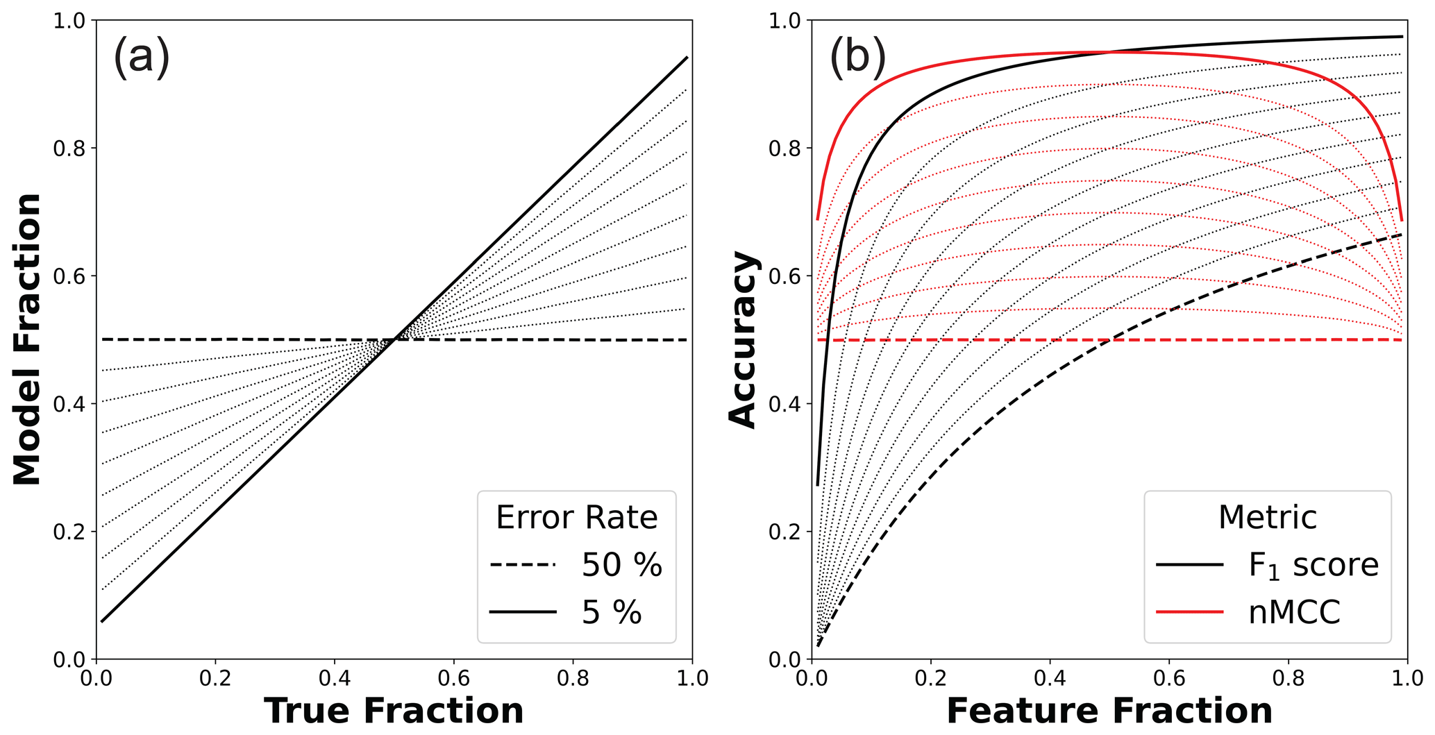
Figure 4 (a) Model feature fractions and (b) associated accuracy scores as a function of the true feature fraction in the random error scenario (1000 × 1000 m map area). In both plots, the minimum and maximum error rates are highlighted, and 5 % increments of error rate are shown as dotted lines. In (a), matching the model fraction to the actual fraction of bedrock is not enforced like in other scenarios (Figs. 3, 5). However, the two fractions are linearly related, and the slope of the relationship is directly related to the error rate (Appendix A). In (b), lower rates of random error amplify the nonlinearity between the F₁ score and feature fraction, while nMCC more uniformly improves across a broad range of feature fractions.

4 Error structure and accuracy

The previous section showed how the F₁ score and nMCC vary as a function of feature prevalence for classifiers that only honored scene-level attributes (i.e., feature fraction) with no predictive skill at identifying feature locations. While this is a useful baseline scenario, a good classifier should identify the locations of features and reproduce scene-level attributes, albeit with some residual error. To illustrate these more realistic conditions, three different error scenarios are presented where the error structure is either random (Sect. 4.1), systematic (Sect. 4.2), or both (Sect. 4.3). While actual sources of error in geomorphic studies are typically more complex, these simple scenarios facilitate interpretation and provide insight into how pixel-level accuracy scores perform when the research design explicitly samples across a gradient in feature prevalence.

4.1 Random error

The first error scenario considered is the situation in which the binary classifier successfully identifies feature locations with a fixed rate of random error (${\stackrel{\mathrm{‾}}{e}}_{\mathrm{r}}$). To create synthetic surfaces of this type, a truth grid is first generated (for Fig. 4 $m=n=$ 1000) for a given feature fraction. Features are assumed to occupy a single pixel, though results are robust to different sizes of incipient features because where error occurs is independent of feature locations. To produce the associated model grid, an error grid is first generated using a different pseudo-random seed than that used to generate the truth data. The continuous values of the error grid are converted to binary classes (0: no error; 1: error) using the specified error rate as the threshold. The error grid is then used to construct the model grid from the truth grid by flipping feature classifications wherever the error grid value equals 1. Note that the maximum error rate shown in Fig. 4 is 50 %. This is the scenario in which the truth and model data are least correlated. Increasing the error rate further will produce increasingly stronger negative correlations between the model and truth data. Once both truth and model grids are generated, the F₁ score and nMCC are calculated. This analysis is done for feature fractions that range from 0.01 to 0.99 and error rates ranging from 5 % to 50 %.

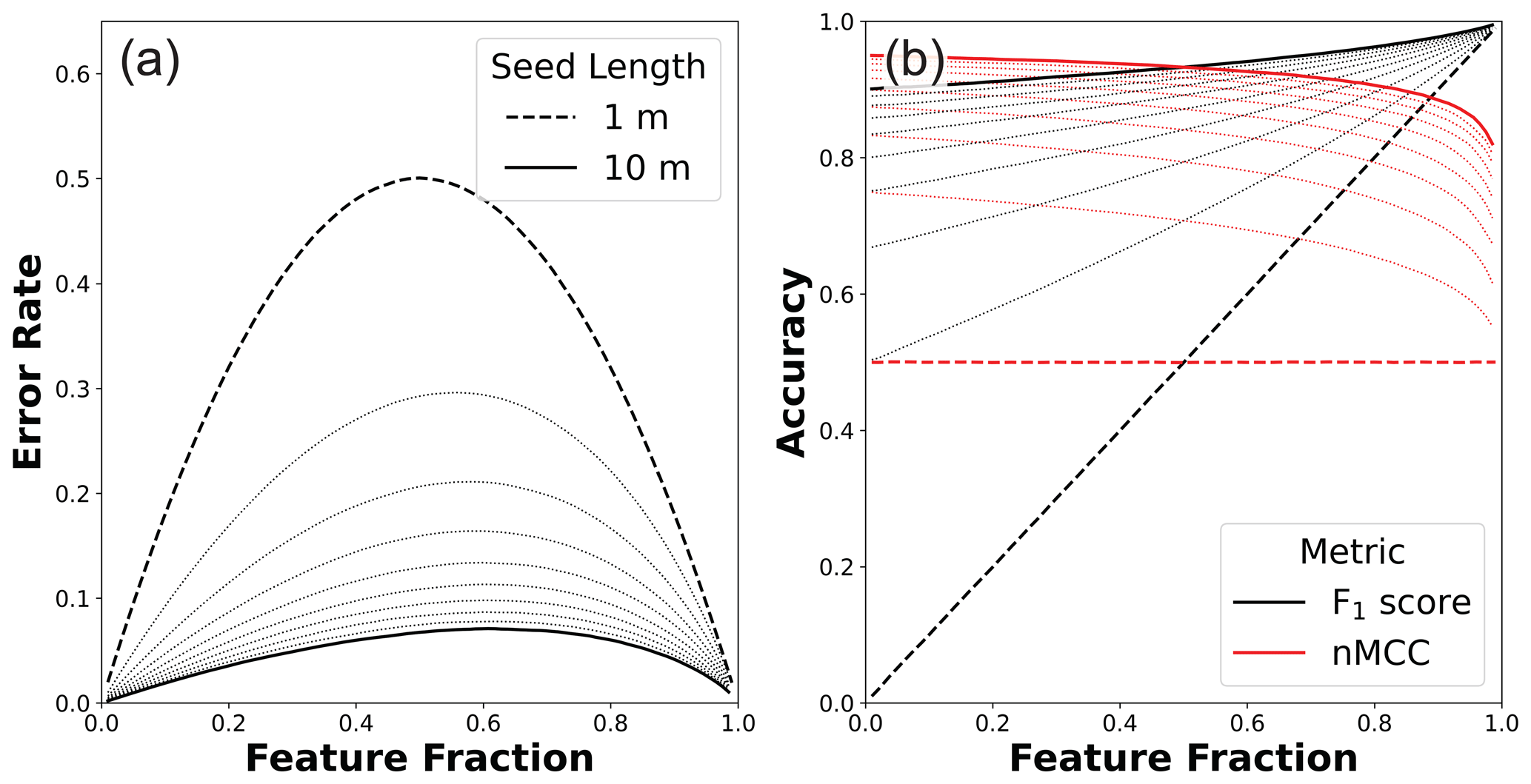
Figure 5 (a) Variable error rates and (b) associated accuracy scores as a function of the true feature fraction for the systematic error scenario (1000×1000 m map areas). In both plots, the minimum and maximum incipient feature lengths are highlighted, and 1 m increments are shown as dotted lines. In (a), the error rate (Eq. 2) is nonuniform with lower rates at both low and high feature fractions. As incipient feature size gets larger, the error rate function becomes increasingly asymmetrical with peak values of 0.5 and 0.66 in bedrock for 1 and 10 m long seeds, respectively. In (b), the nonuniform error rates lead to more linear relationships between the F₁ score and feature fraction than in the case of random error (Fig. 4b). In contrast, nMCC shows modest negative relationships with feature fraction for all incipient feature sizes.

Figure 4 shows the results of this analysis for 10 numerically simulated error rates. Results can be derived analytically from Eqs. (5)–(7) and the imposed random error rate (Appendix A). However, presenting the results from numerical surfaces (1) ensures that synthetic scenes adequately sample population statistics and (2) facilitates integration with scenarios that include non-random error (Sect. 4.3). As should be expected, Fig. 4 shows that accuracy scores increase as error rates go down. However, the sensitivity of these scores is not uniform with respect to feature fraction. Much like in the previous scenario (Fig. 3), F₁ scores always monotonically improve with increasing feature fraction. Note here, though, that the worst random error case (Fig. 4 dashed black line; 50 % error rate) is not equivalent to the case in which the model is independent from the truth data (i.e., the solid black line in Fig. 3). In the random error scenario, model data are correlated with, but not equal to, actual feature fractions (Fig. 4a). The fixed error rate preferentially modifies the larger frequency class near the end-member cases of zero and full coverage of the surface by features. This is most easily envisioned at the limits of feature abundance. If the actual surface is all features, then the random error model will produce matrix pixels in proportion to the error rate. Similarly, if the actual surface is all matrix, then the random error model will produce feature pixels in proportion to the error rate. For this error scenario, the slope of the relationship between modeled and actual feature fractions equals $\mathrm{1}-\mathrm{2}{\stackrel{\mathrm{‾}}{e}}_{\mathrm{r}}$ (Appendix A). The symmetry of the sensitivity of nMCC to a uniform, random error rate allows for comparison of map accuracies across a wide range of feature abundances, specifically over the domain over which nMCC is approximately invariant (Fig. 4b). In contrast, disentangling the spurious correlation between the F₁ score and feature fraction interacts with the preferential modification of classes in a complex way, leading to increasing nonlinearity for better classifiers with lower error rates.

4.2 Systematic error

The second error scenario considered is the situation in which the binary classifier successfully identifies features with some imposed systematic error. This scenario is motivated by the common challenge of aligning two datasets collected using different sensors or collected at different times (e.g., Bertin et al., 2022). To create synthetic surfaces of this type, a truth grid is first generated (for Fig. 5 $m=n=$ 1000) for a given feature fraction and incipient feature size. Incipient features are randomly distributed throughout the model domain. To produce the associated model grid, a copy of the truth grid is linearly offset by 1 pixel to the right in the x direction, though results are insensitive to the direction of the shift. By using wrap-around boundaries, synthetic truth and model grids always have identical feature fractions. Note that the systematic error rate (${\stackrel{\mathrm{‾}}{e}}_{\mathrm{s}}$) is not constant and is instead a function of the feature fraction, the magnitude of the systematic offset, and the shape and size of features. Once both truth and model grids are generated, the F₁ score and nMCC are calculated. This analysis is done for feature fractions that range from 0.01 to 0.99 and for incipient feature sizes that range from 1×1 to 10×10 m².

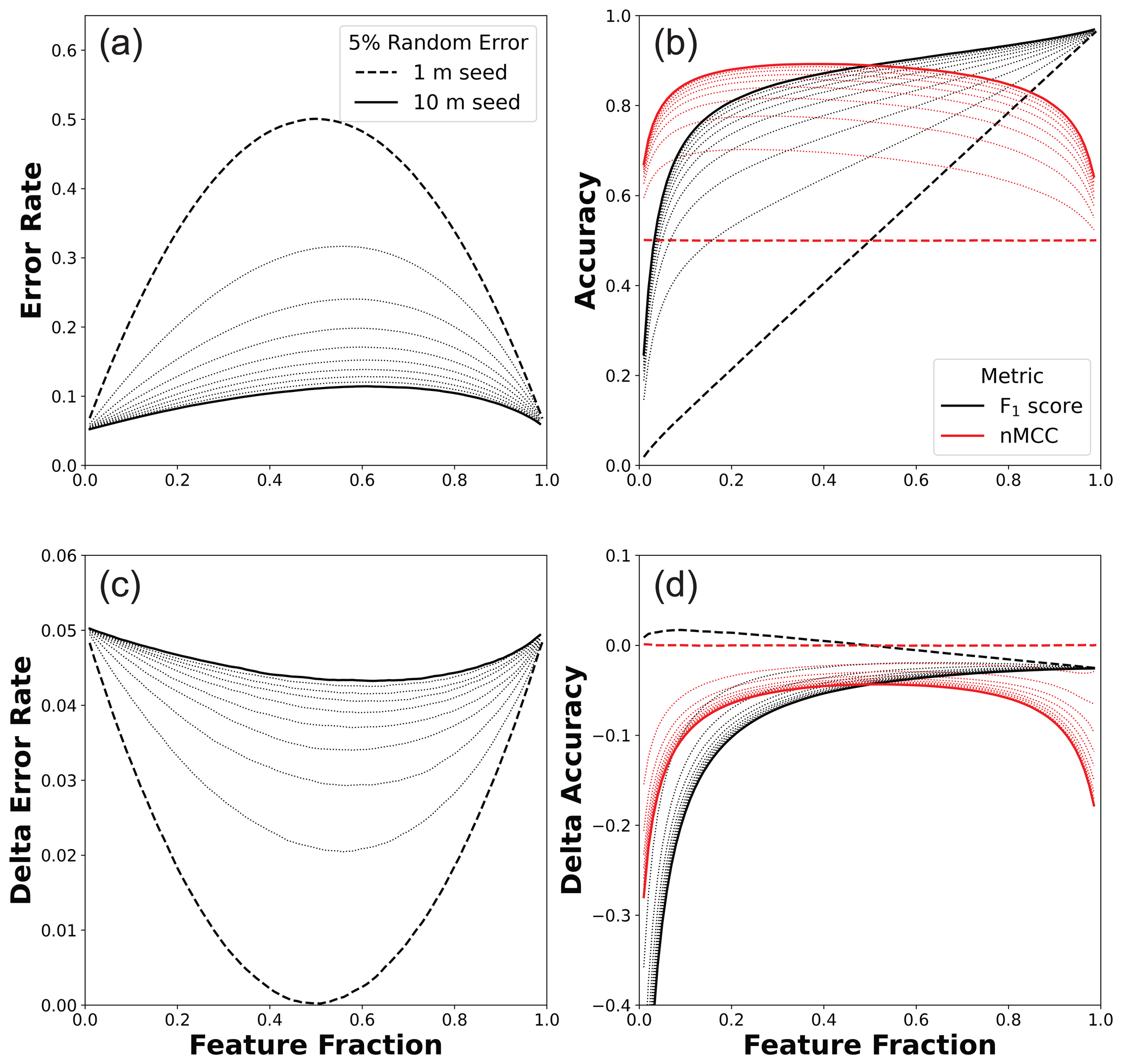
Figure 6 (a) Variable error rates and (b) associated accuracy scores as a function of the true feature fraction for the systematic plus random error scenario (1000×1000 m map areas). These panels are analogous to Fig. 5a and b but now include a 5 % random error term. Differences in (c) error rates and (d) accuracy scores between this scenario and systematic error alone (Fig. 5) are shown to enable comparison. In (c), the additional 5 % random error term is linearly added to the systematic error term at the end-member cases of zero and total feature coverage. The random error translates into something less than 5 % for intermediate cases with minima near zero for 1 m seeds and 0.043 for 10 m seeds. In (d), nMCC exhibits strong reductions from systematic error alone near end-member cases (high negative values) and a muted, more uniform reduction at intermediate values.

Figure 5 shows the results of this analysis for 10 different incipient seeds that span from 1 to 10 m in length (1 to 100 m²). While results throughout this paper are discussed in terms of a scale typical to airborne lidar (i.e., 1 m spatial resolution), the relationships shown here are better cast as the ratio of the incipient feature scale (i.e., seed length in pixels) to the error scale (1 pixel length) where the feature detection limit is 1 pixel. When systematic error is of the order of feature length, systematic error mimics the case in which the truth and model data are independent (e.g., compare long dashed lines in Fig. 5b to solid lines in Fig. 3c–d). As the systematic error gets small with respect to the incipient feature size, both the F₁ score and nMCC improve. The largest improvements occur for small incipient feature sizes and at low feature fractions (Fig. 5b). When feature fractions are low, the error is largely due to the geometric effect of the shift of individual square objects surrounded by matrix. As feature fraction increases, incipient objects increasingly coalesce into a smaller number of objects, and the error is set by these more complex geometries (see discussion in Sect. 5.2). Figure 5a shows that increasing the incipient feature size leads to lower error rates and increasing asymmetry in the error rate function, where the highest error is biased towards higher feature abundances. These error rate functions manifest as a modest negative relationship between nMCC and feature fraction regardless of incipient feature size (Fig. 5b). The asymmetric error structure also impacts the F₁ score, albeit in a way that is much harder to diagnose due to the spurious correlation between the F₁ score and feature fraction (Figs. 3–4). The notion of systematic error in scene-level mapping was envisioned for situations in which co-registration error between the remote sensing data used to map the truth and the remote sensing data used to build the classifier produces a systematic, translational offset. Strictly speaking then, this synthetic scenario represents the case in which a translational offset is the same for all scenes, a plausible situation if the truth and model data for different scenes were acquired at the same time and in the same way. However, even under the less stringent condition in which co-registration errors are oriented differently in different scenes (i.e., due to different acquisition parameters and times), the relationships shown in Fig. 5 will still hold as long as the magnitude of the systematic error is similar across scenes and there is no preferred orientation to feature objects.

4.3 Random plus systematic error

The third error scenario considered is the situation in which the binary classifier is systematically offset from the truth grid with an additional random error term. To create synthetic surfaces of this type, a truth grid is first generated (for Fig. 6 $m=n=$ 1000) for a given feature fraction and incipient feature size. Incipient features are randomly distributed throughout the model domain. To produce the associated model grid, a copy of the truth grid is first linearly offset by 1 pixel to the right in the x direction using a wrap-around boundary condition. A random error grid is then generated using a different pseudo-random seed than that used to generate the truth data. The continuous values of the error grid are converted to binary classes (0: no error; 1: error) using a random error rate of 0.05 as a threshold. The error grid is used to flip classifications in the offset feature grid wherever the error grid value equals 1. Note that feature fractions in the model need not match the truth data, and error rates are now a function of the feature fraction, the magnitude of the systematic offset, the size and shape of features, and the random error rate. Once both truth and model grids are generated, the F₁ score and nMCC are calculated. This analysis is done for feature fractions that range from 0.01 to 0.99 and incipient feature sizes that range from 1×1 to 10×10 m².

Figure 6 is analogous to Fig. 5 with error rates (Fig. 6a) and accuracy scores (Fig. 6b) plotted as a function of feature fraction for different incipient features sizes. The random error rate sets the minimum observed error and contributes to the total error in a nonuniform way. This is because the random error term can flip values where systematic error has occurred (i.e., both sources of error can combine to produce true positives). Figure 6c–d show the differences in error rates and accuracy scores, respectively, between the systematic plus random error scenario shown here (Fig. 6a–b) and systematic error alone (Fig. 5a–b). The addition of random error is relatively more influential in cases in which the classifier is more accurate (i.e., larger incipient features) and near end-member bedrock fractions (i.e., zero and total coverage of features). For a given incipient feature size, the minimum error added by the random error rate of 0.05 occurs at intermediate bedrock fractions and ranges from near zero for 1 m long seeds to 0.043 for 10 m long seeds. Figure 6 shows that the relative importance of random versus systematic error changes as a function of feature fraction. Because random error is the dominant term of the total error rate near the end-member cases of zero and total feature coverage, it leads to correspondingly large reductions in nMCC (Fig. 6d). In contrast, at intermediate bedrock fractions there is a slight negative slope to nMCC like that observed in the systematic error scenario (Fig. 5b). This is because reductions in nMCC induced by random error at intermediate feature fractions are relatively smaller, approximately invariant across a broad range of fractions, and symmetrical with respect to feature fraction (Fig. 6d). While only one random error rate is shown, this example illustrates how the complex interactions between random and systematic error need to be simulated to understand their implications for pixel-level accuracy scores.

5 Discussion

Whether mapping orographic gradients in bedrock exposure (Rossi et al., 2020), characterizing precipitation controls on termite mound density (Davies et al., 2014), or inferring how wind extremes induce tree throw frequencies (Doane et al., 2023), lidar topography has revolutionized our ability to map differences in the density of fine-scale features. None of these examples used pixel-level accuracy scores in their analyses. In fact, it is not immediately apparent how well such methods would perform even if the authors had adopted pixel-level accuracy assessment. For those geomorphic studies that have used pixel-level accuracy scores on lidar-based classifiers (e.g., Bunn et al., 2019; Clubb et al., 2014; Milodowski et al., 2015), it is also not obvious how accuracy scores are expected to vary as a function of feature prevalence. To help address this challenge, this paper presented a suite of synthetic scenarios that show how the F₁ score and Matthews correlation coefficient (MCC) perform across gradients in feature prevalence when the error structure between model and truth data are known. While the scenarios are simple, they provide insight into how well suited, and under what conditions, two of the most widely used accuracy metrics can be used when data are imbalanced (Sect. 5.1). The systematic error scenarios further revealed a strong sensitivity of accuracy metrics to the shape and size of feature objects (Sect. 5.2). Finally, the results from synthetic scenarios are used to provide a tentative set of best practices for using pixel-level metrics in geomorphic studies (Sect. 5.3).

5.1 Accuracy assessment for imbalanced mapping tasks

One main goal of this study was to understand the sensitivity of the F₁ score and MCC to feature prevalence. It is useful for accuracy scores to be invariant with respect to feature fraction under a given error structure so that classified scenes can be calibrated and validated using a wide range of geomorphic settings. For example, the Matthews correlation coefficient (MCC) and its normalized equivalent (nMCC) readily diagnosed the case of independence between truth and model data across the full range of feature abundances (red lines in Fig. 3). In contrast, a spurious correlation between feature abundance and the F₁ score was only exacerbated by adding scene-level constraints to this case (black lines in Fig. 3). Because the F₁ score only considers true positives, false positive, and false negatives, it is an asymmetric accuracy metric (Table 1). Asymmetry refers to the fact that the score is dependent on the choice of target class. All pixel-level assessments that do not consider all four components of the confusion matrix (e.g., precision, recall, F measures, receiver operating characteristic curves) are asymmetric. Asymmetric metrics may not be problematic if one outcome is much more important than its alternative due to its consequences (e.g., a medical diagnosis). However, for many of the geomorphic mapping applications posed here, the relative importance of one class over the other is unclear (e.g., bedrock versus soil, mound versus inter-mound, incised versus un-incised). Successfully identifying both the occurrence and non-occurrence of features is important. In multi-class accuracy assessment, it is common to calculate a “macro” F₁ score, which is the arithmetic mean of F₁ scores for all classes. This macro averaging can also be applied to binary tasks by calculating the F₁ score for the alternative cases when target classes are swapped (Sokolova and Lapalme, 2009). While a macro F₁ score for binary classification is symmetrical and easy to calculate, adoption of this approach is still relatively rare (Chicco and Jurman, 2020).

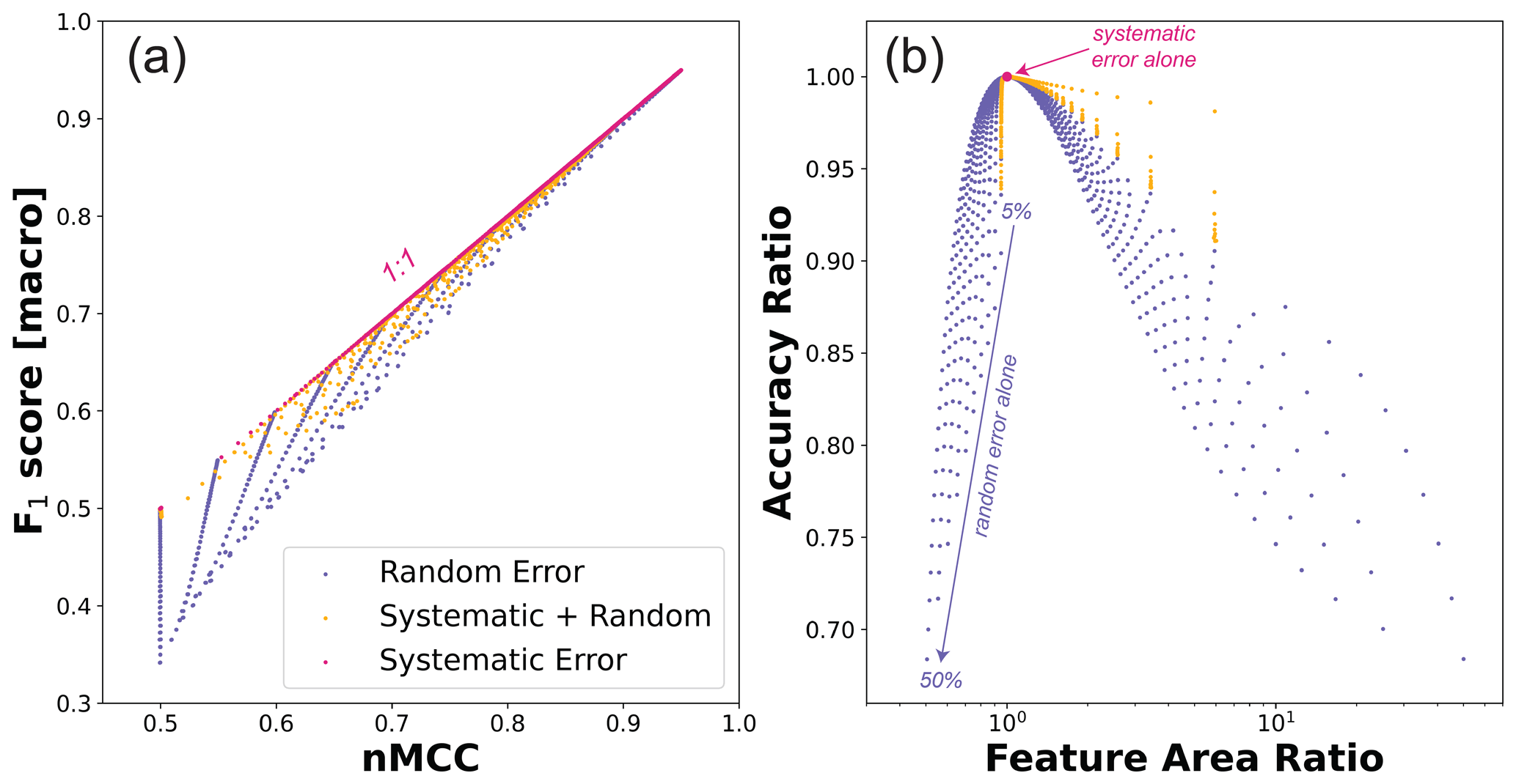
Figure 7 (a) Relationship between nMCC and macro F₁ score for all the error scenarios posed in this study. (b) Ratio of accuracy scores (nMCC $/$ macro F₁ score) as a function of feature area ratios (model area $/$ true area). In (a), the macro score is the arithmetic mean of the two F₁ scores calculated when classes are swapped. In (b), the ratio of scores is plotted as a function of the ratio of feature areas to show that when the model and truth data exhibit different scene-level properties (e.g., feature areas or fraction), the macro F₁ score produces lower values. The systematic error scenario enforced the property that model and truth data match scene-level fractions, which is why they all plot at the coordinates [1,1]. The other error scenarios often produced mismatches between scene-level feature fractions. In these cases, the accuracy metrics are only equivalent when the scene-level fractions match.

Figure 7 shows how macro F₁ scores compare to nMCC for each of the error scenarios considered in this paper. This modified version of the F₁ score addresses the problem of asymmetry and produces similar values to nMCC when the error is small. In the systematic error scenario, the scene-level fraction of bedrock in the model data is identical to the truth data. This leads to a direct correspondence between the nMCC and macro F₁ score (red symbols in Fig. 7). However, for the scenarios that include a fixed rate of random error, the macro F₁ scores generally plot below the 1:1 relationship (Fig. 7a). In these scenarios, accuracy metrics are only equivalent in cases in which the scene-level fractions are the same between the model and truth data (Fig. 7b). Notably, the systematic plus random error scenario produces accuracy metric ratios (Fig. 7b) closer to unity than random error alone for feature area ratios greater than 1 (low feature fractions). When feature area ratios are less than 1 (high feature fractions), accuracy ratios instead follow the trend defined by random error alone. Two important insights can be gleaned from Fig. 7: (1) even though the macro F₁ score addresses the problem of asymmetry, it penalizes random error more than nMCC, and (2) the mismatch between the macro F₁ score and nMCC is encoding disparities between scene-level and pixel-level measures of accuracy, albeit in a highly nonlinear way. Given that the macro F₁ score produces stronger sensitivity than nMCC to the random error scenarios (i.e., accuracy ratios < 1), nMCC should still be favored as a more stable metric when calibrating and validating feature classifiers across gradients in feature prevalence. However, and despite its relative success, caution is still warranted in comparing nMCC across gradients in feature fraction. Uniform, random error preferentially modifies the dominant class, leading to strong reductions in accuracy near end-member cases (Fig. 4; Appendix A). Even for relatively accurate classifiers, random error limits the domain over which nMCC is comparable (e.g., accuracy scores for 5 % random error stabilize between ∼ 20 % and 80 % feature abundances; Fig. 4).

The synthetic scenarios posed in this study were motivated by tasks for which differences in scene-level feature abundances are driven by differences in geomorphic setting (e.g., due to climate, ecology, material property, erosion rate). As such, the synthetic surfaces generated for this analysis assumed that feature locations were homogeneously distributed within each scene (like the Mima mounds in Fig. 1a). The key difference across scenes was feature prevalence, which was used to identify how sensitive accuracy metrics are to imbalanced data. However, the sensitivity of accuracy metrics to feature fraction also provides insight into how metrics might behave when features are heterogeneously distributed within a scene (like the bedrock and gully erosion maps in Fig. 1b–c). While it is beyond the scope of this analysis to systematically explore this, a simple thought experiment using the scenes generated from this study show why within-scene heterogeneity might be important to pixel-level accuracy assessment. There are many combinations of scenes with different feature fractions that can merge into a larger one with the same feature fraction. Table 2 shows a suite of examples that each produce 50 % feature coverage.

Table 2 Merged scenes that produce 50 % feature area* (scene 1 %/scene 2 %).

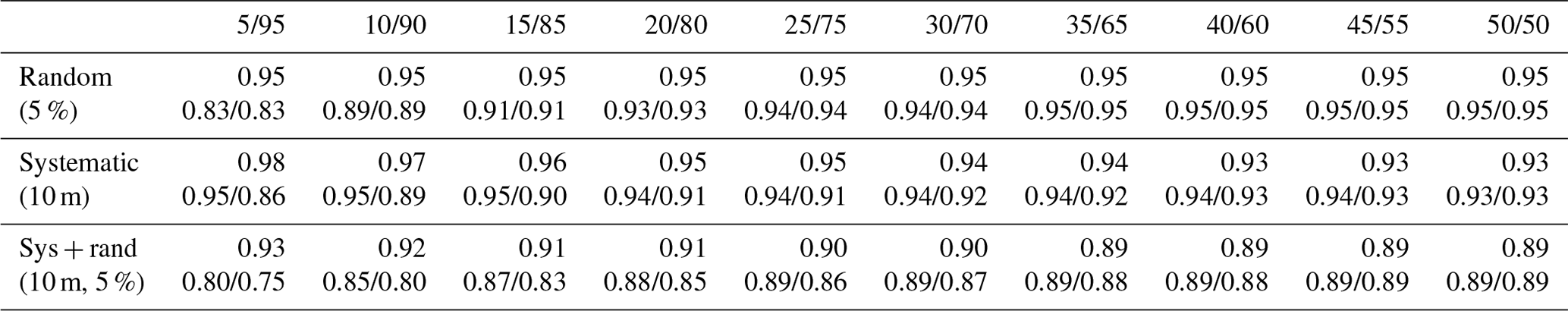
^* The top row is the nMCC of merged scenes. The bottom row is the nMCC of each individual scene that was merged.

The merging of scenes in Table 2 helps illustrate how heterogeneous feature distributions may impact nMCC. For the random error scenario, the strong sensitivity to end-member cases is erased, and nMCC is uniform across all 10 scene mixtures. For the systematic error scenario, accuracy improves for the higher feature fraction portion of the scene, while accuracy marginally decreases for the lower feature fraction portions of the scene. For the systematic plus random error scenario, accuracy improves for both the higher and lower feature fraction portions of the scene. In all cases, nMCC is higher for the merged scenes than for their constituent components, until they converge on each other when fully homogenous. While systematic error clearly induces nonuniform mixing (i.e., merged nMCC varies with different constituent feature fractions), all three cases suggest that heterogeneity generally favors more stable estimates of accuracy by sampling portions of the scene with both more and less abundant features. More thorough examination of this claim is needed. Taken at face value, these results argue that it is better to train a model on all the data at once than on individual scenes with different feature fractions if the source of classification error is expected to be similar. However, scene-level comparisons may provide more insight into variations in the error structure of the classification model itself, which is often poorly constrained.

Taken as a whole, nMCC should be strongly preferred over the F₁ score when building and testing classifiers across gradients in feature abundance, with heterogeneous scenes and pooling of data perhaps favoring more stable assessment. Despite this result, the two scenarios that include systematic error also suggest that asymmetry in accuracy scores is arising in response to the geometries and genesis of features. In these cases, asymmetry is not due to limitations of the accuracy metric itself, but is instead a result of how features are simulated in synthetic examples. Whether the synthetic generative process (i.e., randomly distributed square features of constant size) is representative of real transitions from low to high feature fractions is an open question that likely depends on the feature of interest. Nevertheless, these synthetic examples provide an opportunity to probe how the evolution of feature geometries influence accuracy scores, a topic that is explored in much more depth below.

5.2 Size and shape of features

The focus of this paper has largely been on what to expect from pixel-level accuracy scores when a binary classifier is applied across gradients in feature prevalence. Embedded in this analysis are assumptions for how features emerge at higher abundances. Intriguingly, a negative correlation between nMCC and feature prevalence emerged in scenarios with systematic error, regardless of the incipient feature size (Figs. 5b and 6b). Given that nMCC addresses the problem of asymmetry with respect to target class (Figs. 3c–d and 4b), what causes this asymmetrical sensitivity of nMCC to systematic error? One likely candidate is the simulated changes in feature prevalence entailing a corresponding change in the size and shape of feature objects. A feature object is defined here as a spatially isolated occurrence of the target class (i.e., the ones in a binary classification) enveloped by pixels of non-occurrence (i.e., the zeros in a binary classification). As features become more abundant, small objects coalesce into larger ones. This section probes the role of object size and shape in error by examining how the incipient feature shape interacts with translational error.

5.2.1 Shape and scale of incipient features

All the synthetic scenarios presented above used incipient features with square shapes and whose scale was varied using a single parameter, the incipient feature length. The square geometry was useful because squares are oriented in the same way as the regular grids being used, thus imposing a rotational symmetry to translational offsets. However, other rotationally symmetrical shapes could have been used. Figure 8 shows four alternative shapes whose rotational symmetry makes them insensitive to the direction of translational offset between truth and model data. Because these shapes are constrained by their raster representation, it is hard to create different shapes with the same area when objects are small. For the shapes “square”, “rounded”, “plus”, and “star”, all four shapes have approximately equivalent areas (< 3 % difference) for shape diameters of 6, 7, 10, and 11 pixels, respectively (Fig. 8a). The number of false positives and false negatives for a 1-pixel offset is a function of both the object size and shape (Fig. 8b). As feature objects get larger, the relative error induced by a 1-pixel offset typically goes down. For a given object area, the relative frequency of error induced by a 1-pixel offset appears to be sensitive to the complexity of object boundaries.

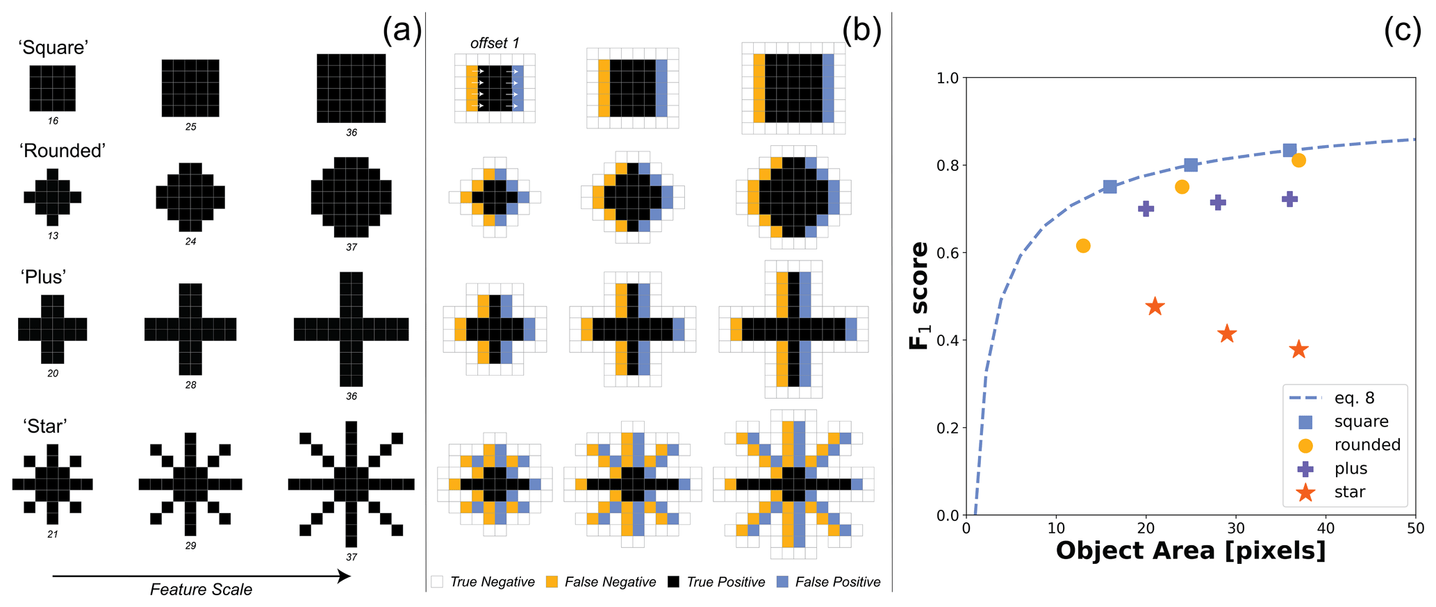
Figure 8 (a) The shape and scale of incipient feature objects directly affect (b) the subsequent frequencies of false negatives (yellow) and false positives (blue) to a 1-pixel translational offset in model classification, (c) which also results in different scaling relationships between object areas and the F₁ score. In (a), four different objects are shown that have either convex (i.e., square, rounded) or concavo-convex (i.e., plus, star) boundaries with respect to the matrix. The object area is reported below each shape in pixels. Note that the smallest “rounded” example is not actually round, but a rotated square. In (b), error classes are shown for a 1-pixel shift to the right. Because shapes are all rotationally symmetric with respect to the four cardinal directions, error rates do not depend on the direction of the shift. Only true negatives that share an edge with the other classes are shown. In (c), the F₁ score for each of the 16 shapes is plotted as a function of the object area. The function describing how the object area and F₁ score vary for square features (Eq. 8) is also plotted as a dashed line for reference.

To help interpret the relative trade-off between object size and shape, Fig. 8c plots the F₁ scores of the example feature objects in Fig. 8a as a function of object area. Due to the symmetry of translational offset, recall, precision, and F₁ score are equivalent for this kind of systematic error. Each of these metrics provides a measure of accuracy induced by feature shape alone, independent of the scene-level abundance of features. The error induced by a 1-pixel shift between truth and model classification can be directly derived for the square case because of its simple geometry. The number of true positives is equal to l²−l, and the number of false positives and false negatives is each equal to l, where l is the length of the square in integer units of pixels. Substituting these terms into Eq. (5) and simplifying yields an equation for the F₁ score specific to square features:

$$\begin{array}{}\text{(8)}& {\mathrm{F}}_{\mathrm{1}}{\mathrm{score}}_{\mathrm{sq}}=\mathrm{1}-{\displaystyle \frac{l}{l^{\mathrm{2}}}}.\end{array}$$

The last term in Eq. (8) explains why accuracy improves as a function of feature area. The area of a square increases faster than its length, thus leading to lower sensitivity to the 1-pixel offset. This ratio is equivalent to the number of pixel edges divided by the total number of pixels for a rasterized shape, which is referred to here as the edge-to-area ratio. The edge-to-area ratio can be calculated for any raster shape and sets how sensitive the F₁ score is to a translational offset. The kinds of shapes differ in how the edge-to-area ratio changes as they get larger, thus defining different scaling relationships between accuracy and feature size (Fig. 8c). In general, concave shapes (i.e., square and rounded) are more conducive to higher F₁ scores. Concavo-convex shapes have more complex boundaries, with some shapes even showing a reduction in accuracy with increasing size (e.g., star shape). Even though the synthetic scenarios used in this study assumed square seeds for their incipient features, the coalescing of these incipient shapes into larger objects means that complex boundaries, and thus increasing edge-to-area ratios, emerge as feature prevalence increases.

5.2.2 Shape and scale of emergent features

In the synthetic scenarios presented above, the minimum feature size is set by the incipient feature length (i.e., 1 to 10 pixels). Because incipient features are placed on the surface randomly, more complex objects are produced where incipient features overlap by chance. To illustrate the implications of this, Fig. 9a shows examples of individual objects that can be generated using square seeds. Examples are organized by incipient feature size (rows) and object areas (columns). Adjacent to each object is the error induced by a 1-pixel shift to the right, with its corresponding F₁ score reported above it. Note that individual objects are not necessarily rotationally symmetric. If an object has a preferred orientation, then error will be enhanced for objects for which the long axis is perpendicular to the translational offset and reduced for objects for which the long axis is parallel to the translational offset. In practice, the sensitivity of error to object orientation is not realized in the synthetic scenarios above because the random placement of features results in objects without a preferred orientation.

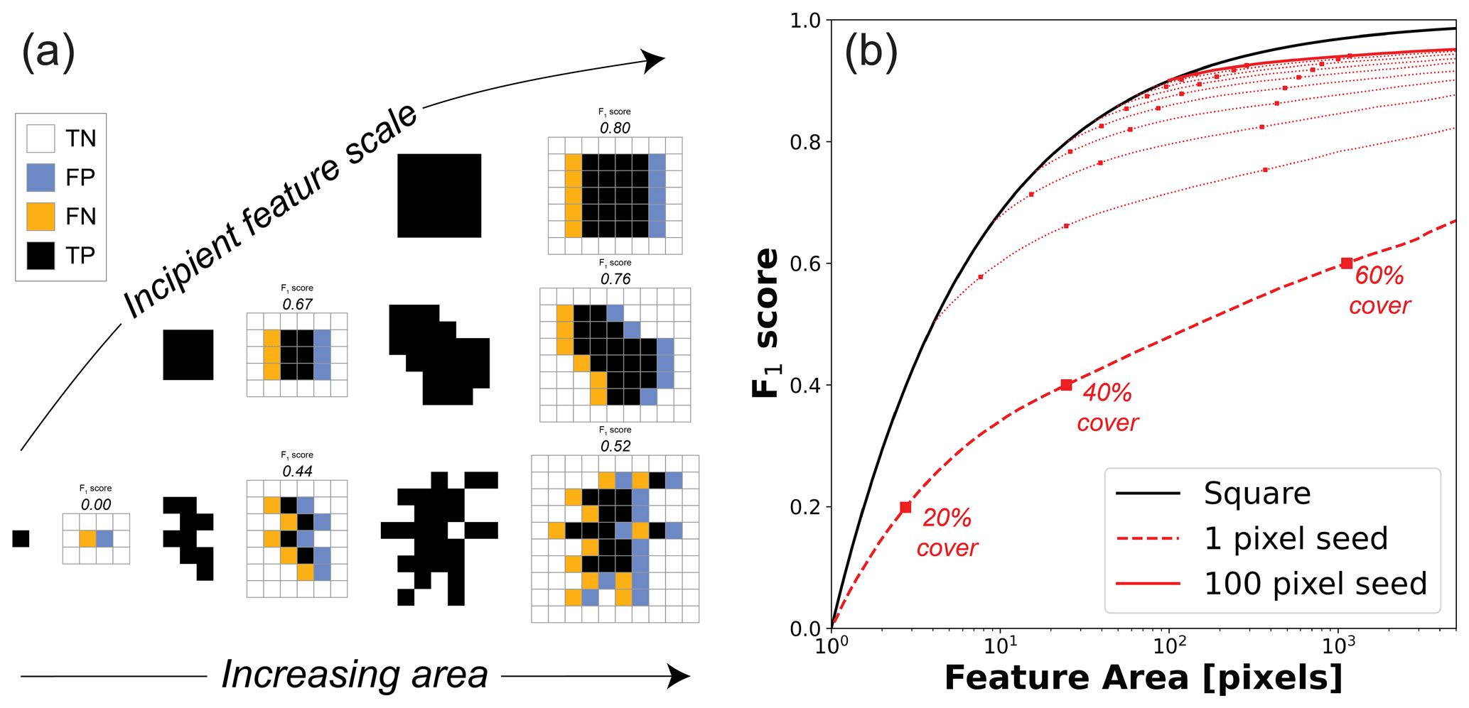
Figure 9 (a) For a given object area, the frequency of false positives and false negatives differs among incipient objects and the emergent objects that coalesce from smaller ones such that (b) F₁ scores increase with average object area more slowly than square objects do in response to a 1-pixel offset. In (a), six permissible object shapes are shown for three different incipient feature sizes (rows) and three different object areas (columns). The incipient feature shape controls both the minimum object size and the complexity of object boundaries. Smaller incipient features can produce more complex shapes and higher error rates for a given feature size (see associated F₁ scores). In (b), the F₁ score is plotted as a function of average object area for the systematic error scenario (Fig. 5). Markers show values at three different feature fractions. The black line is the function describing how the F₁ score responds to a 1-pixel offset for an individual square object (Eq. 8).

While the examples shown in Fig. 9a reiterate the point that error is reduced for larger objects with simpler shapes in response to a 1-pixel offset, it still does not show how object properties vary in the synthetic scenarios presented above. Figure 9b plots the F₁ score as a function of the mean object area for the systematic error scenario. To calculate object areas, the binary map of features (i.e., pixel values equal to one) is segmented into objects. Object segmentation is based on adjacency of the target feature class to at least one of its eight neighbors (see examples in Fig. 9a). Objects can contain holes, but these holes do not contribute to their object area. After segmenting the scene into objects, the average object area is calculated and linked to the F₁ scores reported earlier (Fig. 5). Figure 9b shows that the F₁ score generally improves with increasing object area, albeit in a way that is strongly mediated by the incipient feature size. All lines intersect with the function describing the F₁ score for square features (Eq. 8; solid black line) for the limiting case in which there is only one object in the scene. For any given incipient feature size though, the F₁ score quickly drops off this function due to the increasing complexity of object boundaries. There is a monotonic increase in the F₁ score with average object area and feature prevalence (markers in Fig. 9b) regardless of the incipient feature size. The scenarios above do not produce shapes like the stars shown in Fig. 8. Larger features do lead to higher F₁ scores (Fig. 9b). It was already shown that placing larger features in the landscape improves accuracy in response translational offset (Figs. 5–6). As such, the negative trends in nMCC shown in Figs. 5b and 6b suggest that the net result of increasing the size of objects, for a given incipient seed, is outweighed by the complexity of feature boundaries generated by coalescing them. This analysis suggests that it is paramount to understand the scaling properties of features as they become more prevalent to understand how accuracy scores may be affected by small co-registration errors. Finally, the sensitivity of accuracy metrics to the size and shape of individual features begs important questions as to how stable accuracy metrics are to increasing spatial resolution. As airborne remote sensing is supplemented and superseded by drone-based mapping, there is good reason to believe that the sizes and shapes of better-resolved features may change and thus influence how binary classifiers perform.

5.3 Recommendations and future directions

Many geomorphic tasks share the need for binary classifiers that perform well across gradients in feature abundance. Whether constraining the density of landslide scars, channel erosion, bedrock outcrops, or pit–mound features, geomorphic studies often rely on fine-scale mapping to determine how feature size, extent, and prevalence respond to differences in environmental forcing. There is a general need for classifiers that successfully handle imbalanced data. This paper set out to understand how two widely used pixel-level accuracy metrics perform across gradients in feature prevalence. By using synthetic examples in which the error structure of the data is known, heuristics can be developed for best practices when the research design specifically calibrates and validates binary classifiers across gradients in feature abundance. Four key recommendations emerged.

1. The Matthews correlation coefficient and its normalized equivalent (nMCC) are much better suited than the F₁ score to comparing accuracy scores when feature abundances vary across classified scenes. Even after addressing the problem of asymmetry, the macro F₁ score tends to overpenalize random error.

2. For random error, caution is warranted in interpreting nMCC near the end-member cases of zero and full feature coverage because random error preferentially modifies the dominant class. Though scores are relatively invariant only between ∼ 20 %–80 % feature coverage, this domain might be expanded for scenes with more heterogeneous feature distributions.

3. For systematic error, nMCC is strongly sensitive to the size and shape of individual objects. Larger objects with simpler boundaries are less sensitive to this kind of error because their edge-to-area ratios are small. As such, it is important to characterize both co-registration uncertainty and the attributes of the individual objects being mapped.

4. Before training and testing classifiers on imbalanced data, it is essential to establish baseline expectations for how pixel-level accuracy scores respond to potential sources of error over the range of feature abundances observed. This can be accomplished through numerical simulation.

Simulating a suite of simple scenarios with a known error structure and uniform incipient seeds provided some insight into how pixel-level accuracy metrics behave across gradients in feature prevalence. Real-world applications are decidedly more complex. In the scenarios presented here, increased feature density was simulated by randomly distributing the nuclei of incipient features within the model domain. Such a treatment may be relevant to some applications but is clearly limited. Figure 1 anticipated three clear limitations of simulating features in this way. Many features show evidence of a characteristic size and spacing (e.g., Mima mounds in Fig. 1a), size distributions spread across a wide range of scales (e.g., bedrock exposure in Fig. 1b), and anisotropy (e.g., gully erosion in Fig. 1c). As such, more work is needed to understand how pixel-level accuracy metrics perform on imbalanced data that exhibit these properties. To this end, three promising future research directions are the following.

1. As landscape evolution modeling attempts to keep pace with increasingly higher-resolution observations (Tucker and Hancock, 2010), it also has wide potential for error analysis. Instead of randomly generating features, numerical models can produce more realistic feature distributions that are derived from the relevant geomorphic transport laws at play (Dietrich et al., 2003). A process-based approach towards error assessment could be used to identify under what conditions binary classifiers can be reliably compared across gradients in feature fraction.

2. Pixel-level accuracy scores are built on the confusion matrix, which does not retain the spatial autocorrelation structure or the semantic content of feature objects. Given the importance of the size and shape of features to some error scenarios, the path forward may lie in multi-scale, object-based image analysis (e.g., Drăguţ and Eisank, 2011). Object-based image analysis is on the cutting edge of feature extraction from remote sensing data (Hossain and Chen, 2019). Yet, how to reliably evaluate the accuracy of image segmentation algorithms will require creative rethinking and retooling of standard pixel-level accuracy scores (Cai et al., 2018).

3. Both opportunities above emphasize the overarching challenge of the rapidly changing landscape of data with increasing spatial resolution. Higher-resolution data impact the practical challenge of co-registration error and highlight the more theoretical challenge of semantic vagueness, or the notion that feature boundaries may not be sharply defined (Sofia, 2020). As data resolution increases, traditional methods in image segmentation and binary classification may require new approaches (Zheng and Chen, 2023).

On the one hand, this paper is a call to action on adopting standard methods from the data sciences in research on surface processes. On the other hand, geomorphic questions provide a diversity of real-world use cases in which these “standard” methods can be put to the test and new methods can be developed. As machine learning approaches towards geomorphic mapping proliferate, better understanding is needed of how these methods will perform on the scientific tasks that are currently driving surface process research forward.

6 Conclusions

Pixel-level accuracy assessment provides a powerful tool for understanding how well classifiers built from high-resolution topography are performing. To be most useful, the limitations of commonly used metrics like precision, recall, and F₁ score need to be considered. Classification tasks that span large gradients in feature abundance are particularly vulnerable to biases in these metrics because data are imbalanced and the choice of target class matters. More robust metrics like MCC and nMCC largely address these methodological challenges. However, caution is still warranted in comparing pixel-level scores across gradients in feature density and extent. If error is random and uniform across scenes, then nMCC will dramatically worsen near end-member cases because the more prevalent class is preferentially modified, though this effect may be mediated by pooling data from many different scenes. If the model is systematically offset from the truth grid, then an asymmetrical sensitivity of nMCC can arise depending on assumptions for the genesis and growth of individual features. As the size of individual features increases, there is lower sensitivity to systematic offset. However, if the shapes of features are also getting more complex, then the increased edge-to-area ratio of individual features can counteract and exceed improvements in accuracy associated with larger feature sizes. Though pixel-level metrics used in the machine learning and remote sensing community should be more widely adopted in geomorphic research, further work is needed to understand how different sources of error might decouple pixel-level from scene-level measures of accuracy.

Appendix A: Random error and accuracy metrics

Section 4.1 reported how pixel-level accuracy scores vary as a function of bedrock fraction for a fixed rate of random error. While the synthetic surfaces were generated using Python, the results shown in Fig. 4 can be directly derived from the mean random error rate (${\stackrel{\mathrm{‾}}{e}}_{\mathrm{r}}$) and true feature fraction (f_f) analytically. Under this scenario, the probability of flipping either class is independent of the prevalence and location of features such that we can define the average frequencies for all four components of the confusion matrix. The relative frequencies of each outcome are the product of the average rate of error (or non-error) and the average abundance of the true class. For example, the true positives reflect both the probability of the feature occurring (f_f) and the probability of not being flipped in the model due to random error (i.e., $\mathrm{1}-{\stackrel{\mathrm{‾}}{e}}_{\mathrm{r}}$). The frequencies of all four classification outcomes are as follows:

$$\begin{array}{}\text{(A1)}& {\displaystyle }{f}_{\mathrm{TP}}=\left(\mathrm{1}-{\stackrel{\mathrm{‾}}{e}}_{\mathrm{r}}\right)f_{\mathrm{f}},\text{(A2)}& {\displaystyle }{f}_{\mathrm{FP}}={\stackrel{\mathrm{‾}}{e}}_{\mathrm{r}}{f}_{\mathrm{f}},\text{(A3)}& {\displaystyle }{f}_{\mathrm{FN}}={\stackrel{\mathrm{‾}}{e}}_{\mathrm{r}}\left(\mathrm{1}-f_{\mathrm{f}}\right),\text{(A4)}& {\displaystyle }{f}_{\mathrm{TN}}=\left(\mathrm{1}-{\stackrel{\mathrm{‾}}{e}}_{\mathrm{r}}\right)\left(\mathrm{1}-f_{\mathrm{f}}\right).\end{array}$$

Because we also know that the feature fraction in the model (f_fm) must equal the sum of the fractions of true positives and false negatives, these equations yield the following relationship:

$$\begin{array}{}\text{(A5)}& f_{\mathrm{fm}}=\left(\mathrm{1}-{\stackrel{\mathrm{‾}}{e}}_{\mathrm{r}}\right)f_{\mathrm{f}}+{\stackrel{\mathrm{‾}}{e}}_{\mathrm{r}}\left(\mathrm{1}-f_{\mathrm{f}}\right).\end{array}$$

Equation (A5) can be rearranged and simplified to describe how the model feature fraction is related to the true feature fraction,

$$\begin{array}{}\text{(A6)}& f_{\mathrm{fm}}=\left(\mathrm{1}-\mathrm{2}{\stackrel{\mathrm{‾}}{e}}_r\right)f_{\mathrm{f}}+{\stackrel{\mathrm{‾}}{e}}_{\mathrm{r}}.\end{array}$$

The relationships shown in Fig. 4a (main text) are equivalent to Eq. (A6) for different error rates. That the Python-generated scenes match the analytical solution indicates that the domain used for these synthetic scenes is large enough to adequately sample population statistics. Note that Eq. (A6) provides a prediction for the relationship between true and model bedrock fractions only if error is uniform and random across scenes. In such cases, the average error rate can be directly inferred from both the slope and y intercept of the regression.

Because pixel-level accuracy scores can be derived directly from the confusion matrix, the simplified assumptions of random, uniform error also facilitate prediction for how the F₁ score and nMCC will vary with the true feature fraction. Substituting the values from Eqs. (A1)–(A4) into Eq. (5) (main text) yields

$$\begin{array}{}\text{(A7)}& {\mathrm{F}}_{\mathrm{1}}\mathrm{score}={\displaystyle \frac{\mathrm{2}{f}_{\mathrm{f}}\left(\mathrm{1}-{\stackrel{\mathrm{‾}}{e}}_{\mathrm{r}}\right)}{\mathrm{2}{f}_{\mathrm{f}}\left(\mathrm{1}-{\stackrel{\mathrm{‾}}{e}}_{\mathrm{r}}\right)+{\stackrel{\mathrm{‾}}{e}}_{\mathrm{r}}}},\end{array}$$

which is equivalent to the numerically generated black curves in Fig. 4b. Similarly, substituting Eqs. (A1)–(A4) into Eq. (6) (main text) yields

$$\begin{array}{}\text{(A8)}& \begin{array}{rl}& \mathrm{MCC}=\\ & {\displaystyle \frac{\sqrt{f_{\mathrm{f}}}\times \sqrt{\mathrm{1}-f_{\mathrm{f}}}\times \left(\mathrm{1}-\mathrm{2}{\stackrel{\mathrm{‾}}{e}}_{\mathrm{r}}\right)}{\sqrt{f_{\mathrm{f}}+{\stackrel{\mathrm{‾}}{e}}_{\mathrm{r}}-{\stackrel{\mathrm{‾}}{e}}_{\mathrm{r}}^{\mathrm{2}}-f_{\mathrm{f}}^{\mathrm{2}}-\mathrm{4}{\stackrel{\mathrm{‾}}{e}}_{\mathrm{r}}{f}_{\mathrm{f}}-\mathrm{4}{\stackrel{\mathrm{‾}}{e}}_{\mathrm{r}}{f}_f^{\mathrm{2}}-\mathrm{4}{\stackrel{\mathrm{‾}}{e}}_{\mathrm{r}}^{\mathrm{2}}{f}_{\mathrm{f}}-\mathrm{4}{\stackrel{\mathrm{‾}}{e}}_{\mathrm{r}}^{\mathrm{2}}{f}_{\mathrm{f}}^{\mathrm{2}}}}},\end{array}\end{array}$$

which is equivalent to the numerically generated red curves in Fig. 4b. Though the expression for MCC under random, uniform error is complex, it reveals why there is strong and symmetrical sensitivity near the end-member cases of zero and all bedrock. The numerator in Eq. (A8) decreases faster than the denominator near end-member cases regardless of the average error rate. Since f_f and 1−f_f are complementary and ${\stackrel{\mathrm{‾}}{e}}_{\mathrm{r}}$ is assumed to be constant, this reduction in MCC is also symmetrical around an optimal bedrock fraction of 0.5.