Decadal-scale decay of landslide-derived fluvial suspended sediment after Typhoon Morakot

Landslides influence fluvial suspended sediment transport by changing sediment supply and grain size, which alter suspended sediment concentrations and fluxes for a period of time after landsliding. To investigate the duration and scale of altered suspended sediment transport due to landsliding, we analyzed suspended sediment concentration and water discharge measurements at 87 gauging stations across Taiwan over an 11-year period after Typhoon Morakot, which generated nearly 20 000 landslides in 2009. At each gauging station, we computed annual rating curves to quantify changes over time in the sensitivity of suspended sediment concentrations to water discharge. Among the 40 stations in basins that were impacted by landsliding, the discharge-normalized rating curve coefficient $\stackrel{\mathrm{̃}}{a}$ was higher than that before Morakot by a factor of 5.1±1.1 (mean ± standard error) in 2010, the first year after Morakot. The rating curve exponent b did not decrease at most stations until a year later (2011), when the average b value was lower than that before Morakot by 0.25±0.05. Across the compilation of gauging stations, post-Morakot changes in discharge-normalized sediment concentration ($\stackrel{\mathrm{̃}}{a}$) were positively correlated with landslide intensity for 7 years after Morakot, while post-Morakot changes in the exponent of the discharge–concentration relationship (b) were negatively correlated with landslide intensity from 2011 to 2014. This reflects a tendency for larger changes in $\stackrel{\mathrm{̃}}{a}$ and b to occur in basins with more intense landsliding. At 26 of these 40 stations, elevated values of $\stackrel{\mathrm{̃}}{a}$ declined after the initial post-Morakot peak, consistent with a gradual return to pre-Morakot suspended sediment transport conditions. Exponential regressions to these $\stackrel{\mathrm{̃}}{a}$ values reveal a median characteristic decay time of 8.8 years (interquartile range: 5.7–14.8 years). Values of $\stackrel{\mathrm{̃}}{a}$ increased more and declined faster in basins with more intense landsliding, with a mean characteristic decay time of 6 years in the basins hit hardest by landsliding. Furthermore, changes in $\stackrel{\mathrm{̃}}{a}$ and b tended to be larger in basins with more intense landsliding. At stations that were not impacted or only minimally impacted by landsliding, neither $\stackrel{\mathrm{̃}}{a}$ nor b exhibited systematic responses to Morakot. To quantify the effect of landsliding on sediment discharge, we compared the measured sediment discharges after Morakot to the hypothetical sediment discharges that would have occurred if Morakot had induced no landslides, calculated by applying each station's pre-Morakot rating curve to its post-Morakot water discharge history. This analysis suggests that Morakot-induced landsliding increased sediment discharge by as much as > 10-fold in some basins in the 1–2 years after Morakot. Together, these results indicate that the influence of Morakot-induced landsliding on rating curves was large shortly after Morakot but diminished in less than a decade in most of the study rivers and will be imperceptible in another few decades in all of the study rivers. To the extent that these results are applicable to other landscapes, this suggests that periods of elevated sediment transport efficiency after landsliding should persist for years to decades, even if the landslide deposits persist for centuries to millennia.

1 Introduction

Widespread landsliding events, such as those caused by heavy rainfall (e.g., Milliman and Kao, 2005; Marc et al., 2018; Yamada et al., 2012), can deliver large amounts of sediment to rivers and temporarily elevate suspended sediment concentrations and sediment discharge (e.g., Milliman and Syvitski, 1992; Hovius et al., 2000; Hovius et al., 2011). In fluvial monitoring records, this is often characterized by a brief spike in suspended sediment concentrations followed by a protracted tail of elevated suspended sediment concentrations (e.g., Hicks et al., 2008). In a given river, the duration of the tail depends on the river's ability to transport the landslide-mobilized material and hence on the river’s transport capacity and the size of the landslide deposit accessible to the river. Recent studies have inferred a wide range of recovery times for sediment fluxes responses to landsliding, from several years for suspended sediment fluxes (e.g., Hicks et al., 2008; West et al., 2014; Croissant et al., 2017) to hundreds of years for bedload fluxes (e.g., Yanites et al., 2010).

Questions about the persistent influence of mass wasting on sediment concentrations are particularly relevant in Taiwan, which experiences frequent landsliding due to large rainfall events and large earthquakes. Taiwan is susceptible to frequent landsliding because it is undergoing rapid uplift in response to arc–continent collision between Eurasia and the Philippine Sea Plate (Suppe, 1984) and is one of the most rapidly eroding places on Earth, with denudation rates exceeding 10 mm yr⁻¹ in some areas (Dadson et al., 2003; Fox et al., 2014). In many mountainous regions in Taiwan, rock uplift rates outpace erosion rates by diffusive soil transport, and landslides are the dominant source of hillslope erosion (Hovius et al., 2000). For example, the 1999 magnitude 7.3 Chi-Chi earthquake caused over 20 000 landslides covering over 150 km² (Dadson et al., 2004). Similarly, Typhoon Toraji in 2001 induced > 30 000 landslides, which resulted in > 175 Mt of suspended sediment discharge in 1 d from the Choshui River (Dadson et al., 2005), equivalent to 3 times its annual average sediment load over the period from 1986 to 1999.

In this study, we focus on the responses to landslides induced by Typhoon Morakot (5–9 August 2009). This was the wettest typhoon on record in Taiwan, generating > 3 m of rainfall in the south-central portion of Taiwan (Fig. 1a) and close to 20 000 landslides with a net area > 250 km² (Lin et al., 2011). This disturbance was such that it may have altered the regional microseismicity (Steer et al., 2020), and it resulted in amplified fluvial sediment fluxes in many basins across Taiwan (Kao et al., 2010). Huang and Montgomery (2013) documented fluvial responses to Morakot by analyzing measurements of suspended sediment concentration (C) and water discharge (Q) at 19 gauging stations in southern Taiwan monitored by Taiwan's Water Resources Agency. With these data, they calculated two rating curves of the form C=aQ^b (where a and b are constants) at each station: one for the monitoring period before Morakot, which spanned several decades, and another for the 2 years of post-Morakot measurements that had been made by that time. This revealed that the centered rating curve coefficient a increased and the rating curve exponent b decreased after Morakot at 15 of the 19 study stations, indicating more efficient suspended sediment transport at a given discharge and a smaller sensitivity of C to Q.

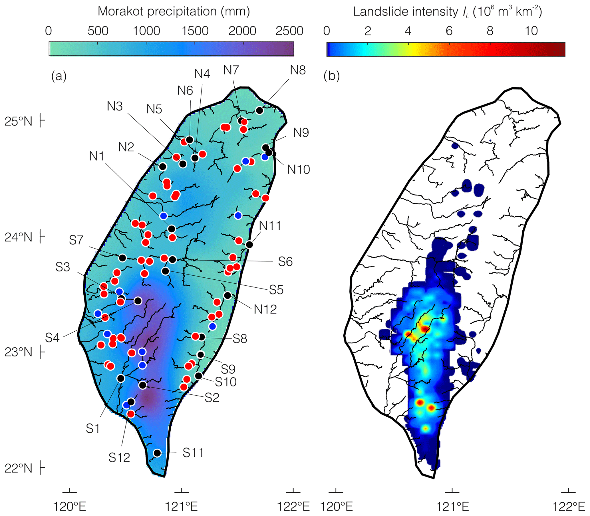
Figure 1 (a) Locations of fluvial gauging stations analyzed in this study. The stations of focus in Figs. 4, 5, 7, and 9 (black dots) are labeled S1–S12 in southern Taiwan and N1–N12 in northern Taiwan. Large red dots indicate stations used to calculate trends in rating curve parameters, and blue dots indicate stations used to compute sediment discharge (Table S1). Contoured colors represent rainfall totals during Typhoon Morakot derived from a kriging-based interpolation of rainfall gauging stations (Water Resources Agency, 2020). (b) Spatial density of landsliding (volume of mobilized material per unit area) smoothed from the compilation in Marc et al. (2018).

Huang and Montgomery (2013) interpreted these changes in the rating curves as reflecting a shift from coarser to finer sediment, which would generate a decrease in b at the same time as an increase in a. This was supported by bed grain size measurements before and after Morakot by the Water Resources Agency in the Beinan River, which revealed a reduction in median grain size at this site after Morakot. Huang and Montgomery (2013) further observed that the magnitude of the grain size fining in the Beinan River would be enough to shift the sediment transport regime from threshold bed (gravel) to live bed (sand), which would increase sediment discharge at low flow. As Huang and Montgomery (2013) noted, although the perturbations to the rating curves were large in many rivers, it was not possible to evaluate how long these perturbations would last, since only 2 years of post-Morakot measurements were available at the time. If these perturbations persisted for long times, then this would imply that large landslide events should generate enduring changes in the sediment transport regime, sediment fluxes, and erosional unloading. If, on the other hand, these perturbations diminished quickly, then large landslide events should only generate elevated sediment fluxes for geologically short times and have little influence on long-term mass fluxes.

Recent advances offer an opportunity to reassess the duration of fluvial responses to Morakot and to quantify the sensitivity of these perturbations to landsliding. Marc et al. (2018) generated a new inventory of Morakot-induced landslides across Taiwan, which provides a comprehensive assessment of landslide volumes (Fig. 1b). In addition, suspended sediment concentrations and discharge have continued to be monitored at many rivers across Taiwan, with more than a decade of measurements now accumulated since Morakot (Water Resources Agency, 2020).

Here we build on Huang and Montgomery (2013) to revisit two questions. (1) How much did Typhoon Morakot affect fluvial suspended sediment fluxes at rivers across Taiwan? (2) How long did these effects last? To address these questions, we analyzed suspended sediment concentration and water discharge measurements at 87 fluvial gauging stations in basins across Taiwan (Water Resources Agency, 2020), which were affected by Morakot to varying degrees. Some of these basins experienced intense landsliding during Morakot and showed major changes in suspended sediment transport after Morakot. Others experienced no landsliding and showed no measurable change in suspended sediment transport after Morakot, offering a baseline point of comparison for basins that experienced widespread landsliding. Collectively, these gauging station records provide a means to quantify erosional responses to Morakot across Taiwan and a means to test the sensitivity of these erosional responses to the intensity of landsliding.

This paper is structured around an analysis of the effects of Morakot-induced landsliding on suspended fluvial sediment fluxes. Section 2 summarizes the gauging station measurements and the methods we used to compute suspended sediment loads and rating curves. Section 3 presents annual estimates of the rating curve parameters, suspended sediment loads, and basin-averaged erosion rates, which reveal spatial and temporal variations in sediment fluxes across Taiwan in the decade after Morakot. Section 4 discusses the duration of the perturbation to the rating curve parameters and their sensitivity to the intensity of landsliding. Together, these results constrain the spatial and temporal extent of suspended sediment responses to Morakot-induced landsliding, and they suggest that elevated suspended sediment concentrations in these basins will dissipate within a few decades.

2 Methods

To quantify the duration of fluvial sediment fluxes affected by Typhoon Morakot, we analyzed monitoring records at 87 river gauging stations (Fig. 1a), all of which were operated by Taiwan's Water Resources Agency (WRA; Water Resources Agency, 2020). Supplement Table S1 lists each gauging station's WRA ID, river name, location, and monitoring duration. The monitoring records at these stations are of variable length, with some dating back to 1948 and others starting as late as 2017. The monitoring records consist of measurements of average water discharge at daily intervals and depth-averaged suspended sediment concentrations at less frequent and irregular intervals (Kao et al., 2005). The median sampling interval for suspended sediment concentrations across all gauging stations is 12 d during the typhoon season (June–October) and 15 d during the rest of the year.

As we describe below, we use the gauging station measurements to create rating curves relating suspended sediment concentration to water discharge, and we use these rating curves to compute suspended sediment discharge at each gauging station during each year of each station's operation (Supplement Tables S1–S5). In Sects. 3–4 we present figures from a subset of 24 stations (Fig. 1a) that collectively span the range of responses across the full set of 87 stations and which therefore illustrate the sensitivity of fluvial suspended sediment fluxes to Morakot-induced landsliding. A total of 12 of the 24 focus stations (labeled S1–S12 in Fig. 1a) are in the southern half of the island, where precipitation during Morakot was highest and where landsliding was most intense. These stations were selected based on the completeness of their monitoring records and because they are in basins with high landslide intensity, and therefore these basins are thought to represent some of the higher responses to landsliding found in the southern part of the island. In these basins, the volume of landslide-mobilized material per unit drainage area ranged from 440 to 2.7×10⁵ m³ km⁻². The other 12 stations (N1–N12) are farther north in Taiwan, where precipitation during Morakot was less intense and landsliding was less common. These basins were selected based on the completeness of their monitoring records and are representative of a typical response for northern stations. A total of 8 of these 12 basins had no Morakot-induced landsliding, and in the remaining 4 basins, the volume of landslide-mobilized material per unit drainage area ranged from 4 to 34 m³ km⁻². These provide a baseline against which the responses at stations S1–S12 can be compared.

The focus stations in the north and south share similar characteristics, with the exception of the rainfall and landslide intensity received during Morakot. For example, the southern and northern focus stations have similar drainage areas (north median = 445 km², range = 104–1512 km²; south median = 512 km², range = 77–2942 km²) and discharge distributions (Fig. S1 in the Supplement). Meanwhile, their upstream areas experienced different amounts of precipitation during Morakot (north median = 0.47 m, range = 0.25–0.89 m; south median = 1.31 m, range = 0.63–2.03 m), as well as landslide intensity (north median = 0 m³ m⁻², range = 0–3.4×10⁻⁵ m³ m⁻²; south median = 0.04 m³ m⁻², range = $\mathrm{4.42}\times {\mathrm{10}}^{-\mathrm{4}}$ to 0.27 m³ m⁻²).

The fluvial monitoring records are of variable completeness. Temporal gaps are present in every gauging station's records, with gaps as short as several days to as long as 50 years. On average across all the study gauging stations, 92 % of the days in the monitoring period have discharge measurements. For stations whose early records include large temporal gaps decades before Morakot, we only compute rating curves in time periods with a minimum of five suspended sediment concentration measurements. Among the 24 focus stations, the average number of suspended sediment concentration measurements per year ranges from 15.0 to 29.7.

2.1 Estimating rating curve parameters and suspended sediment loads

A river's suspended sediment load Q_s [M T⁻¹] can be calculated as the product of volumetric water discharge Q [L³ T⁻¹], water density ρ_w [M L⁻³], and suspended sediment concentration C [M M⁻¹] (Eq. 1).

$$\begin{array}{}\text{(1)}& Q_{\mathrm{s}}=CQ{\mathit{\rho }}_{\mathrm{w}}\end{array}$$

At the study gauging stations, Q was measured every day but C was measured less frequently, so direct measurements of Q and C cannot be used to calculate Q_s every day. In such cases, a common approach is to estimate daily values of C by applying a power-law rating curve relating C to Q (Eq. 2; e.g., Ferguson, 1986; Syvitski et al., 2000; Gao, 2008).

$$\begin{array}{}\text{(2)}& C=a{Q}^b\end{array}$$

Here b is a dimensionless constant that describes the sensitivity of C to Q, and a is a constant with dimensions of T^b L^−3b that describes the concentration of suspended sediment at a given Q. At the study gauging stations, the reported measurements of C are in units of parts per million (ppm) and those of Q are in units of m³ s⁻¹ (Water Resources Agency, 2020), and we assume ρ_w=1000 kg m⁻³, so the units of a are ppm s^b m^−3b.

Our goal is to quantify the influence of Morakot-induced landsliding on suspended sediment transport by tracking the evolution of Q_s and the rating curve parameters over time. To do this, we applied a commonly used methodology based on a modified version of Eq. (2) to calculate annual estimates of the suspended sediment load and the rating curve parameters. This involved two steps before calculating values for the rating curve parameters.

The first step is centering the logged discharge data (see Fig. 2 for an example), which we did following Cohn et al. (1992). This reduces the influence of estimates of b on estimates of a, which can confound efforts to compare rating curve parameters at different stations or different times (e.g., Syvitski et al., 2000; Warrick, 2015). This involved calculating the center of the log₁₀(Q) data with Eq. (3) – which we denote as center(log₁₀(Q)) – and subtracting it from the log₁₀(Q) data over the time period of interest.

$$\begin{array}{}\text{(3)}& \begin{array}{rl}\mathrm{center}& \left({\log }_{\mathrm{10}}\right(Q\left)\right)=\mathrm{mean}\left({\log }_{\mathrm{10}}\right(Q\left)\right)\\ & +{\displaystyle \frac{{\sum }_{k=\mathrm{1}}^N\left({\log }_{\mathrm{10}}\right(Q)-\mathrm{mean}({\log }_{\mathrm{10}}\left(Q\right)){)}^{\mathrm{3}}}{\mathrm{2}{\sum }_{k=\mathrm{1}}^N\left({\log }_{\mathrm{10}}\right(Q)-\mathrm{mean}({\log }_{\mathrm{10}}\left(Q\right)){)}^{\mathrm{2}}}}\end{array}\end{array}$$

Here, N is the number of discharge measurements and mean(log₁₀(Q)) is the mean of the log-transformed discharge data.

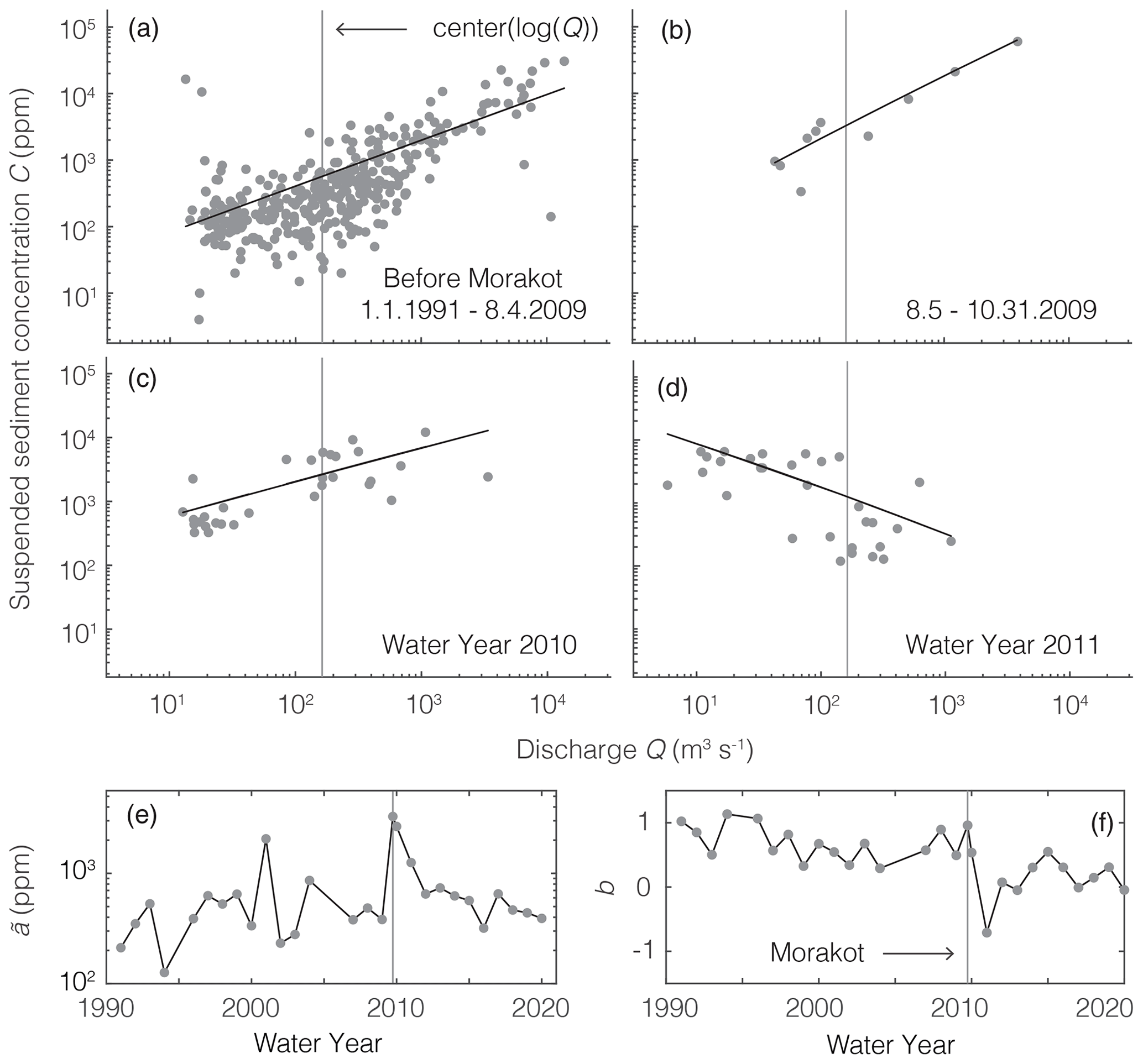
Figure 2 Example of measurements of suspended sediment concentration and water discharge before Morakot (a) and after Morakot (b–d) at station S1 in the Gaoping River (Fig. 1; Water Resources Agency, 2020). Vertical lines show the center of the log-transformed discharge data over the entire monitoring period, which is the discharge at which the rating curve parameter $\stackrel{\mathrm{̃}}{a}$ is determined (Eq. 3). (e, f) Estimates of rating curve parameters $\stackrel{\mathrm{̃}}{a}$ and b at this station from 1991 to 2020. These show the variability in annual estimates of $\stackrel{\mathrm{̃}}{a}$ and b and the influence of Morakot on $\stackrel{\mathrm{̃}}{a}$ and b at this station.

After centering the discharge, we estimated the rating curve parameters by applying the adjusted maximum likelihood estimation (AMLE) method of Cohn et al. (1989) to measurements of log₁₀(C) and the centered discharge log₁₀(Q) – center(log₁₀(Q)). Graphically, this is analogous to a linear regression through log-transformed C and Q data normalized by center(log₁₀(Q)). The resulting parameter values are for the regression line's slope (b) and intercept evaluated at center(log₁₀(Q)). The intercept shares the same units as C (here, ppm) and is denoted $\stackrel{\mathrm{̃}}{a}$ to distinguish it from a in Eq. (2). This is beneficial because it reduces the effects of the artifactual dependency of a on b that would have resulted from regressing log₁₀(C) against the uncentered log₁₀(Q) data and thus simplifies comparison of $\stackrel{\mathrm{̃}}{a}$ values estimated at different times or stations. This method is identical to the AMLE method implemented in the Load Estimator computer program (LOADEST; Runkel et al., 2004), which is based on Cohn et al. (1989). To facilitate comparison of the rating curve parameter values among different stations and different times, we report estimates of $\stackrel{\mathrm{̃}}{a}$ throughout this study.

We applied this approach to each year's C and Q data at each station to compute annual estimates of the rating curve parameters, which permitted quantification of changes in the rating curves over time. To ensure that each year's estimate of $\stackrel{\mathrm{̃}}{a}$ at a given station can be straightforwardly compared to the other annual estimates of $\stackrel{\mathrm{̃}}{a}$ at the same station, we subtracted the same center(log₁₀(Q)) value from each year's log₁₀(Q) measurements at that station. To obtain a common value of center(log₁₀(Q)) to apply to each year at a given station, we applied Eq. (3) to all the discharge measurements over the gauging station's entire monitoring period. The resulting values of center(log₁₀(Q)) for each station are tabulated in Table S2. The methodology is summarized in the example shown in Fig. 2.

The second step we applied in these calculations is a correction for log-transformation bias in estimates of Q_s. To make this correction, we followed the minimum-variance unbiased estimator method (MVUE) of Cohn et al. (1989). We used this method and the daily measurements of Q to calculate daily estimates of Q_s corrected for log-transformation bias. We used the method of Gilroy et al. (1990) to estimate the uncertainty in the suspended sediment load, following the implementation in LOADEST (Runkel et al., 2004). We calculated annual suspended sediment loads over each water year (1 November–31 October) by summing the daily estimates of Q_s over the year. For days without Q measurements, we assigned the year's average daily Q_s value.

After computing Q_s at each gauging station, we computed basin-averaged erosion rates E [L T⁻¹] by dividing Q_s by the drainage area A upstream of the gauging station and an assumed bedrock density ρ_r of 2700 km m⁻³, where drainage areas and flow-routing information were extracted from MERIT Hydro (Yamazaki et al., 2019) and used in subsequent calculations.

$$\begin{array}{}\text{(4)}& E={\displaystyle \frac{Q_{\mathrm{s}}}{{\mathit{\rho }}_{r}A}}\end{array}$$

These represent the spatially averaged erosion rate associated with the suspended sediment load. Because these do not include fluvial mass fluxes associated with bedload or dissolved loads, these values of E represent a lower bound on total basin-averaged erosion rates. For context, Dadson et al. (2003) estimated that bedload from high mountainous rivers could account for 30±28 % (95 % CI) of the total sediment discharge.

Some basins contained multiple gauging stations along the same river. This yielded estimates of Q_s in the catchment draining into the downstream gauging station as well as in the smaller catchment draining into the upstream gauging station, which is contained within the larger catchment. In these situations with nested catchments, we used Eq. (5) to calculate E for the portion of the large basin that is not contained within the smaller tributary basin (e.g., Hu et al., 2021). For example, if we denote the area of the catchment draining into the downstream gauging station A₁, the area of the tributary catchment draining into the upstream gauging station A₂, and the suspended sediment loads from these stations Q_s1 and Q_s2, respectively, then the average erosion rate E₁ over the portion of A₁ that is not part of A₂ is

$$\begin{array}{}\text{(5)}& E_{\mathrm{1}}={\displaystyle \frac{Q_{\mathrm{s}\mathrm{1}}-Q_{\mathrm{s}\mathrm{2}}}{{\mathit{\rho }}_r(A_{\mathrm{1}}-A_{\mathrm{2}})}}.\end{array}$$

To quantify year-to-year variations in sediment fluxes over time, we applied Eqs. (1)–(5) to each gauging station's measurements of Q and C during each water year. This yielded annual estimates of $\stackrel{\mathrm{̃}}{a}$, b, Q_s, and E at each gauging station. We also applied this method to the entire period of C and Q measurements before Morakot at each gauging station to calculate the rating curve parameters based on all pre-Morakot data, which we denote ${\stackrel{\mathrm{̃}}{a}}_{\mathrm{pre}}$ and b_pre (Table S2). These serve as a baseline to compare post-Morakot values of $\stackrel{\mathrm{̃}}{a}$ and b against. Lastly, we applied Eqs. (1)–(5) to two portions of the 2009 water year, one before Morakot (1 November 2008 to 4 August 2009) and one after Morakot began (5 August to 31 October 2009). This isolated the response to Morakot in the first few months after the typhoon from the portion of the 2009 water year that preceded the typhoon.

2.2 Estimating impacts of Morakot on sediment discharge

We aim to quantify the effects of Morakot-induced landsliding on suspended sediment loads over the decade after Morakot. For rivers heavily affected by landsliding, this necessitates quantifying changes in rating curves before and after Morakot. For rivers whose rating curves do not change during a given storm, it may be sufficient to apply the same rating curve to discharges before and after the storm (e.g., Gao, 2008). For other rivers, however, typhoons can alter a river’s rating curve such that the sediment load associated with a given water discharge differs before and after the typhoon (e.g., Kao et al., 2005; Hovius et al., 2000; Fig. 3). In such cases, applying a river's pre-typhoon rating curve to post-typhoon discharge measurements would yield errors in estimates of post-typhoon suspended sediment concentrations and sediment discharge.

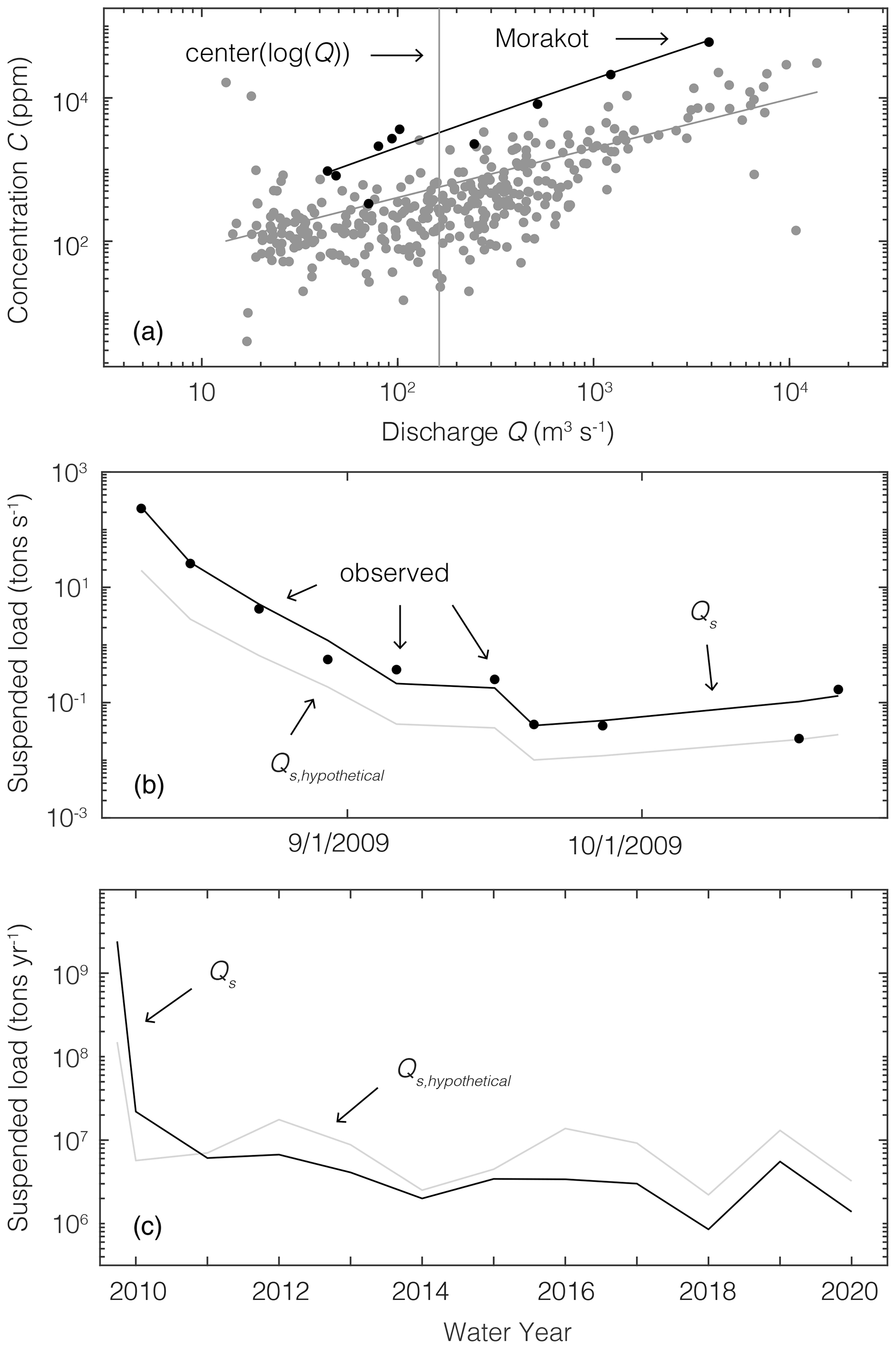
Figure 3 Example of the approach for estimating the effects of Typhoon Morakot on suspended sediment discharge Q_s. (a) Concentration C and discharge Q measurements at station S1 in the Gaoping River (Fig. 1) before Morakot (gray dots; 1 January 1990–4 August 2009) and during the portion of water year 2009 after Morakot began (black dots; 5 August–31 October 2009). Regression lines are inferred rating curves for these time periods. The vertical line is at center(log₁₀(Q)) (Eq. 3). (b) Black dots show observed Q_s on days with measurements of both C and Q during the post-Morakot portion of the 2009 water year. The black line shows Q_s estimated by applying the post-Morakot rating curve (black line in panel a) to discharge measurements. The gray line shows the hypothetical Q_s that would be obtained if the pre-Morakot rating curve (gray line in panel a) were applied to the same discharge measurements. Applying the pre-Morakot rating curve to the post-Morakot discharges would systematically underestimate sediment discharge. (c) Sediment loads at S1 estimated by applying the pre-Morakot rating curve (gray line) and the annual post-Morakot rating curves (black line) to Q measurements. At this site, Q_s exceeds Q_{s,hypothetical} for less than 2 years after Morakot.

Estimates of a river’s annual sediment load are sensitive not just to typhoon-induced changes in the rating curve parameters, but also to the magnitude–frequency distribution of discharge that the river experiences after a typhoon (e.g., Kirchner et al., 2011). For example, if precipitation happens to be lower the year after a typhoon than the year before it, then sediment loads may be lower the year after the typhoon than the year before it, even in rivers in which the rating curve coefficient is higher after a typhoon. Accounting for these temporal variations in discharge is particularly important in Taiwan, where precipitation rates have been highly variable over time. For instance, cumulative rainfall in a given month in a given basin has varied by an order of magnitude or more from year to year (Kao et al., 2005; Yu et al., 2006).

This implies that the effects of Typhoon Morakot cannot be determined by directly comparing a river’s sediment loads before and after Morakot. Instead, to quantify the effect of Morakot on sediment loads, we compared two estimates of the annual sediment load. The first is determined with the conventional application of post-Morakot rating curves to the post-Morakot discharge history, as described in Sect. 2.1. We calculated a rating curve for each post-Morakot water year based on the year’s roughly biweekly C measurements and concurrent Q measurements (Fig. 3a). Then, we applied each year’s rating curve to that year’s time series of daily Q measurements to estimate daily Q_s values (Fig. 3b). Summing the daily Q_s values over each year yielded our best estimates of the annual Q_s (Fig. 3c).

The second estimate is a hypothetical suspended sediment load, Q_{s,hypothetical}, which is meant to answer the following question: what would the post-2009 sediment loads have been if Morakot had not occurred but the rivers had experienced the same discharge history that did occur after Morakot? We calculated Q_{s,hypothetical} by applying the same methodology applied in Sect. 2.1 to the post-Morakot discharge history, except that each estimate used the pre-Morakot values ${\stackrel{\mathrm{̃}}{a}}_{\mathrm{pre}}$ and b_pre, rather than computing new values of $\stackrel{\mathrm{̃}}{a}$ and b each year. Finally, we summed the daily estimates of Q_{s,hypothetical} over each water year to obtain estimates of the annual Q_{s,hypothetical} (Fig. 3c), taking the ratio of the annual Q_s and Q_{s,hypothetical} to be a measure of Morakot's effect on annual suspended sediment discharge.

2.3 Basin-averaged landslide intensity

To quantify the intensity of landsliding in drainage basins upstream of the gauging stations, we used landslide volumes in the inventory of Marc et al. (2018). In this study, Marc et al. (2018) mapped the areas of Morakot-induced landslide scars A_L in Formosat-2 aerial imagery at 8 m multispectral (2 m panchromatic) resolution and estimated landslide volume V_L with Eq. (6) (Larsen et al., 2010):

$$\begin{array}{}\text{(6)}& V_{\mathrm{L}}=c{A}_{\mathrm{L}}^p,\end{array}$$

where the sole parameters are the scaling coefficient c and exponent p. In the landslide catalog in Marc et al. (2018), the calculation of V_L accounts for amalgamated landslide polygons, where it is assumed that each landslide has an elliptical shape and a mean width calculated with the formula proposed and validated by Marc et al. (2018). These calculations also involved estimating scar area using a mean length to width ratio derived from a global database of 277 landslide scars with volumes ranging from 1000 m³ to 1 km³ (Domej et al., 2017). In this catalog, landslide volumes were calculated with Eq. (6) with parameters for shallow landslide scars of $p=\mathrm{1.262}\pm \mathrm{0.009}$ and log₁₀(c) $=\mathrm{-}\mathrm{0.649}\pm \mathrm{0.021}$ and for bedrock landslide scars of $p=\mathrm{1.41}\pm \mathrm{0.02}$ and log₁₀(c) $=\mathrm{-}\mathrm{0.63}\pm \mathrm{0.06}$ (Larsen et al., 2010). We use the landslide volume estimates from Marc et al. (2018) directly.

We calculated the basin-averaged landslide intensity I_L [L³ L⁻²] for each station as the total upstream landslide volume (summed over all landslides) divided by the drainage area A.

$$\begin{array}{}\text{(7)}& I_{\mathrm{L}}={\displaystyle \frac{\sum V_{\mathrm{L}}}{A}}\end{array}$$

3 Results

3.1 Rating curve parameters $\stackrel{\mathrm{̃}}{a}$ and b

At most of the southern stations, values of $\stackrel{\mathrm{̃}}{a}$ increased rapidly within 1 year after Morakot and then declined over the following decade (Fig. 4). At six of the eight southern stations with data in the post-Morakot portion of 2009 (S1–S2, S5–S7, S12), values of $\stackrel{\mathrm{̃}}{a}$ in the post-Morakot portion of 2009 were higher than ${\stackrel{\mathrm{̃}}{a}}_{\mathrm{pre}}$ (the pre-Morakot average value of $\stackrel{\mathrm{̃}}{a}$) by an average factor of 3.4 (range 1.4–8.8). At the other two stations (S3–S4 in the Bazhang River basin), values of $\stackrel{\mathrm{̃}}{a}$ in the post-Morakot portion of 2009 declined slightly to 0.7–0.8 times that of ${\stackrel{\mathrm{̃}}{a}}_{\mathrm{pre}}$. At the remaining four southern stations (S8–S10 in the Beinan River and S11 in the Sizhong River), no data were collected from June 2009 until January 2010, which prevents calculation of $\stackrel{\mathrm{̃}}{a}$ and b values during this time. In water year 2010, the first time $\stackrel{\mathrm{̃}}{a}$ can be estimated at these four stations, values of $\stackrel{\mathrm{̃}}{a}$ are higher than ${\stackrel{\mathrm{̃}}{a}}_{\mathrm{pre}}$ by an average factor of 14 (range 8.1–22).

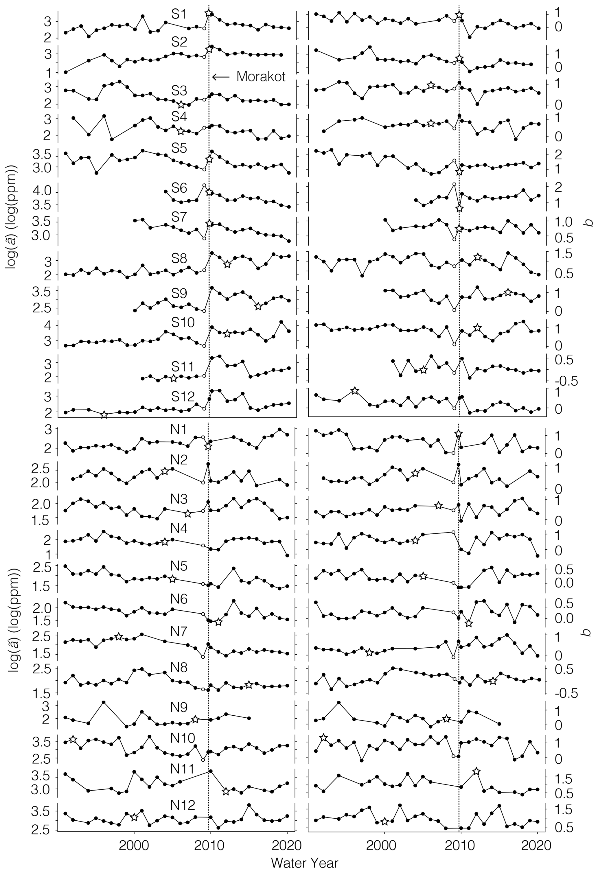
Figure 4 Annual estimates of rating curve parameters $\stackrel{\mathrm{̃}}{a}$ and b at the southern stations (S1–S12), where Morakot-induced landsliding was common, and the northern stations (N1–N12), where it was not. Vertical lines indicate the timing of Morakot. At 11 of the 12 southern stations, $\stackrel{\mathrm{̃}}{a}$ increases immediately after Morakot relative to its pre-Morakot 2009 value (open circles) and then declines. b does not respond systematically among the southern stations. By contrast, at the northern focus stations, where landslide intensity was smaller (Table S2), $\stackrel{\mathrm{̃}}{a}$ and b show smaller responses to Morakot. Maximum Q during this period is represented by the white stars and does not coincide with large changes in $\stackrel{\mathrm{̃}}{a}$ and b at most stations.

By contrast, values of $\stackrel{\mathrm{̃}}{a}$ at the northern stations appear to be largely unaffected by Morakot (Fig. 4; Table S3). The average value of $\stackrel{\mathrm{̃}}{a}/{\stackrel{\mathrm{̃}}{a}}_{\mathrm{pre}}$ across the 12 northern stations in the post-Morakot portion of 2009 is less than 1, and at 9 of the 12 northern stations, the first post-Morakot values of $\stackrel{\mathrm{̃}}{a}$ are smaller than ${\stackrel{\mathrm{̃}}{a}}_{\mathrm{pre}}$. At the remaining three stations, values of $\stackrel{\mathrm{̃}}{a}$ exceed ${\stackrel{\mathrm{̃}}{a}}_{\mathrm{pre}}$ by a factor of 1.3 (N3) to 2.1 (N2) in the post-Morakot portion of 2009 and by a factor of 2.9 (N11) in 2010 – substantially smaller than the average post-Morakot increases in $\stackrel{\mathrm{̃}}{a}$ at the southern stations. Unlike at the southern stations, $\stackrel{\mathrm{̃}}{a}$ does not change systematically over time after Morakot at the northern stations.

As described in Sect. 2.1, we split the 2009 water year into pre-Morakot and post-Morakot portions, which permitted the first few months after Morakot to be isolated from the pre-Morakot portion of the water year. To identify these time periods visually in Fig. 4, the pre-Morakot portion of 2009 is plotted as an open circle and the post-Morakot portion of 2009 is plotted on the vertical line marking the time of Morakot. These values of a and b in the early portion of 2009 are distinct from a_pre and b_pre, which are based on the measurements from all years before 2009. Splitting 2009 like this grouped most of the typhoon season into the post-Morakot portion of the year and excluded most of the typhoon season from the pre-Morakot portion of the year. While this could account for the observation that $\stackrel{\mathrm{̃}}{a}$ is higher during post-Morakot 2009 than it was before Morakot at some stations, we consider this unlikely. At many of the stations, the value of $\stackrel{\mathrm{̃}}{a}$ in post-Morakot 2009 is within 0.1 log units of that in 2010 – much closer than it is to the average value of $\stackrel{\mathrm{̃}}{a}$ in the years leading up to Morakot (e.g., at stations S1–S4 and S6–S7; Fig. 4). If the high $\stackrel{\mathrm{̃}}{a}$ values in post-Morakot 2009 were only a result of splitting the year in two, then, all else being equal, $\stackrel{\mathrm{̃}}{a}$ at the southern stations in 2010 ought to have been substantially lower, closer to the average $\stackrel{\mathrm{̃}}{a}$ value before Morakot.

Unlike values of $\stackrel{\mathrm{̃}}{a}$, values of b across the southern stations did not change systematically immediately after Morakot (Fig. 4). Instead, b increased at some stations and decreased at others. At the southern stations, the average b values in the post-Morakot portion of 2009 and in 2010 were 0.84 and 0.83, respectively, both slightly higher than the average b_pre of 0.81 before Morakot. In the post-Morakot portion of 2009, b was lower than b_pre at three of the eight southern stations with measurements. In 2010, b was lower than b_pre at 5 of the 12 southern stations (Tables S2, S4). Thus, b decreased after Morakot at fewer than half of the southern stations in both 2009 and 2010, despite widespread landsliding in these basins.

The largest decreases in b did not occur until 2011, when b was smaller than b_pre at 10 of the 12 southern stations. In 2011, the average difference between b and b_pre at the southern stations was −0.38 and as large as −1.40 (station S1). At some of these stations, values of b remained lower than b_pre from 2011 through 2020 (S1, S12), while and at other stations, b returned to approximately b_pre in 4 to 7 years (S2, S4, S5, S11).

To put these changes into perspective, consider that the average b value in 2009 and 2010 is in the 54th and 58th percentile compared with pre-Morakot historical values in the north and south focus stations, respectively. Then, from 2011 to 2015, the average b value in the southern focus stations was in the 21st percentile of their respective historical values, while the northern stations were on average in the 54th percentile. Thus, persistently lower values of b appeared in several basins with intense landsliding, but not until the second year after Morakot.

By comparison, across the northern focus stations, where Morakot-induced landsliding was minimal, the average value of b dropped from 0.59 before Morakot to 0.29 in 2010 – a greater decrease than the southern stations experienced during the same time frame, on average. Together, these observations show that some of the stations exhibited a post-Morakot decline in b similar to that documented by Huang and Montgomery (2013), while others did not.

3.2 Suspended sediment discharge Q_s

At 11 of the 12 southern stations (all but S8), suspended sediment discharge increased within 1 year of Morakot relative to average values before Morakot (Fig. 5). At nine of these stations, suspended sediment discharge dropped within 1–2 years after Morakot, and at the remaining two stations (S9 and S10), suspended sediment discharge remained high for 3–4 years. At stations S1–S7, sediment discharge peaked in the post-Morakot portion of water year 2009 (6 August to 31 October 2009). At stations S9–S12, sediment discharge peaked in 2010. For stations S9–S11, we cannot rule out the possibility that Q_s peaked in the post-Morakot portion of water year 2009 given the absence of measurements at these stations during this time.

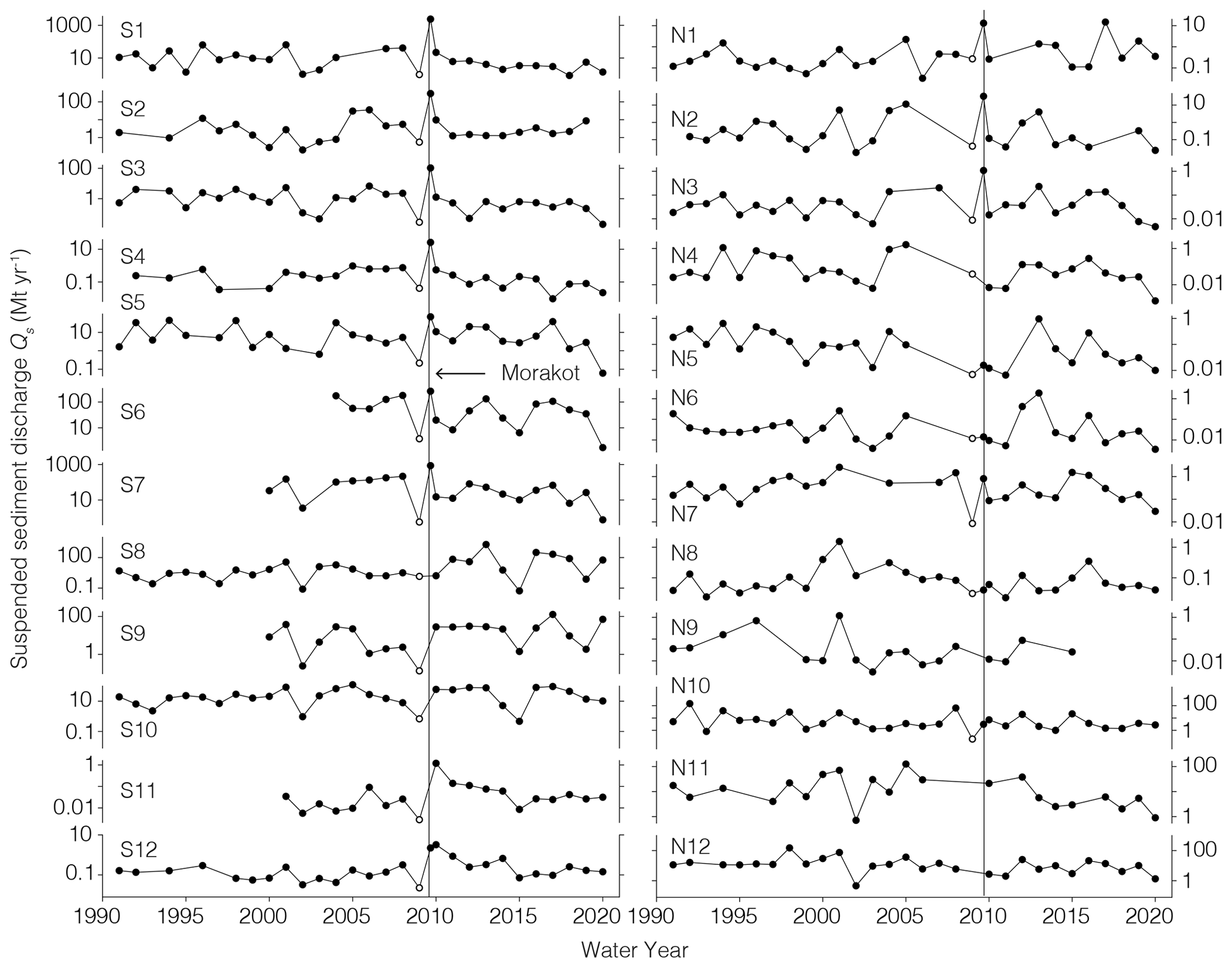
Figure 5 Suspended sediment discharge from 1991 to 2020 at the southern (left) and northern (right) gauging stations (Fig. 1). The vertical line in 2009 shows the time of Typhoon Morakot. The open circle in 2009 represents the pre-Morakot portion of the water year, and the filled circle on the Morakot line represents the post-Morakot portion of the water year. At most of the southern stations, suspended sediment discharge increased greatly during Morakot, then tapered off shortly afterwards. By contrast, at most of the northern stations, suspended sediment discharge did not change during Morakot.

The post-Morakot peaks in Q_s were large, and we compare them to a more “typical” year by comparing to the pre-Morakot median. The median was used for comparison in this case because of the heavy-tailed frequency of events, which can skew individual years to have extreme annual loads (e.g., Dadson et al., 2003). For the stations with peaks in Q_s in the post-Morakot portion of 2009 (S1–S7), Q_s during this time was 2.1–222 times higher than the median Q_s before Morakot. For the stations with peaks in Q_s in 2010 (S9–S12), Q_s during this time was 3.4–84 times higher than the median Q_s before Morakot. The rapid drop-off in Q_s after Morakot was largely due to the influence of discharge Q on estimates of Q_s (Eq. 1; Fig. S2). For example, at site S1, the maximum daily discharge in water year 2010 was only 18 % of what it was during Morakot, and in 2011 it was only 13 %. The total sediment discharged at S1 in water years 2010 and 2011 was only 4 % and 1 %, respectively, of the total during the last 3 months of water year 2009, which included Morakot. All but one of the other southern stations show similarly smaller discharge in 2010 and 2011 compared to 2009, station S12. With the exception of this station, which had a higher sediment load in 2010 than 2009 post-Morakot, the annual sediment discharge at all stations in both 2010 and 2011 was less than 25 % of the sediment discharge in August–October 2009.

In Fig. 5, each water year is indicated with a filled circle except the pre-Morakot portion of the 2009 water year, which is indicated with an open circle. At most stations, estimates of Q_s in the pre-Morakot portion of the 2009 water year are lower than those before and after it. This is largely because this portion of the water year does not include some of the typhoon season, which tends to have more large precipitation events. At most of our study stations, river discharge Q is smaller during this portion of the water year than it is during the typhoon season, which results in a smaller Q_s (Eq. 1).

3.3 Annual erosion rate estimates

We used the estimates of Q_s at all 87 stations to calculate the basin-averaged erosion rate E each year after Morakot. Because these are based on suspended sediment discharge, they do not account for additional mass fluxes as bedload and should therefore be considered minimum bounds on E (Dadson et al., 2003). Figure 6 shows that E varies greatly in time and space across Taiwan. In some small catchments in a given year, E was exceptionally rapid. For example, the sediment discharge from the small basin above station 1660 H010 on the Erhjen River in the post-Morakot portion of 2009 is equivalent to > 10³ mm of basin-averaged erosion, well above the pre-Morakot median of 25 mm yr⁻¹. In other nested catchments, high Q_s values at an upstream station are paired with low Q_s values at a downstream station on the same river in the same year, implying negative values of E in Eq. (5) and hence net deposition in the downstream portion of the basin that year. For example, the Beinan River basin, which contains stations S8–S10, shows an initial decline in erosion rates from 2010 to 2011. Beginning in 2011, erosion rates in the upstream portions of this basin increase dramatically and continue into 2013. Net deposition accumulates downstream, after which the basin returns to nearly uniform net erosion. Similarly, erosion rates in the downstream portion of the Zhuoshui basin (which contains sites S5–S7) decrease dramatically starting in 2010, resulting in net deposition downstream for the remainder of the years analyzed. Together, the panels in Fig. 6 show that most of the island is dominated by net erosion most years and that the fastest erosion occurred in the first few months after Morakot in many regions.

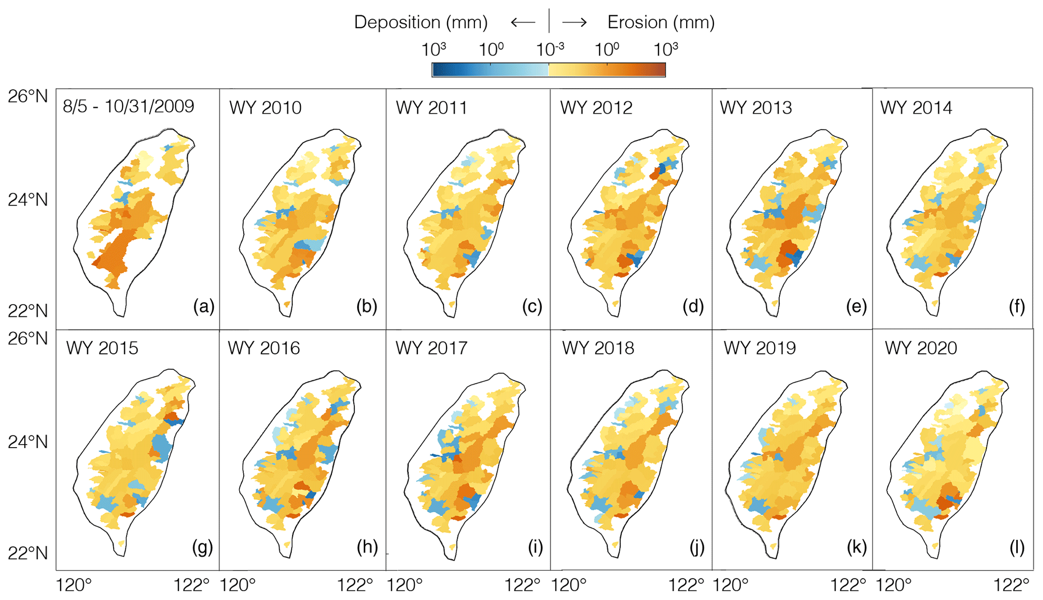
Figure 6 Basin-averaged erosion (yellow-red) and deposition (blue) in the first 3 months after Morakot (a) and each water year (1 November–31 October) after that until 2020 (b–l), calculated with Eqs. (4)–(5). This shows that most of Taiwan was dominated by net erosion most years after Morakot and that in many places the fastest erosion happened in the first few months after Morakot.

3.4 Gain in suspended sediment discharge

Figure 7 shows that, at the southern stations, Q_s was larger than Q_{s,hypothetical} at some stations in some years and smaller than it at other stations and in other years. For example, at station S1, Q_s was 16 times larger than Q_{s,hypothetical} in the post-Morakot portion of 2009 and 4 times larger than it in 2010. At station S6, by contrast, Q_s was half as large as Q_{s,hypothetical} in the post-Morakot portion of 2009 and 2 times larger than it in 2010.

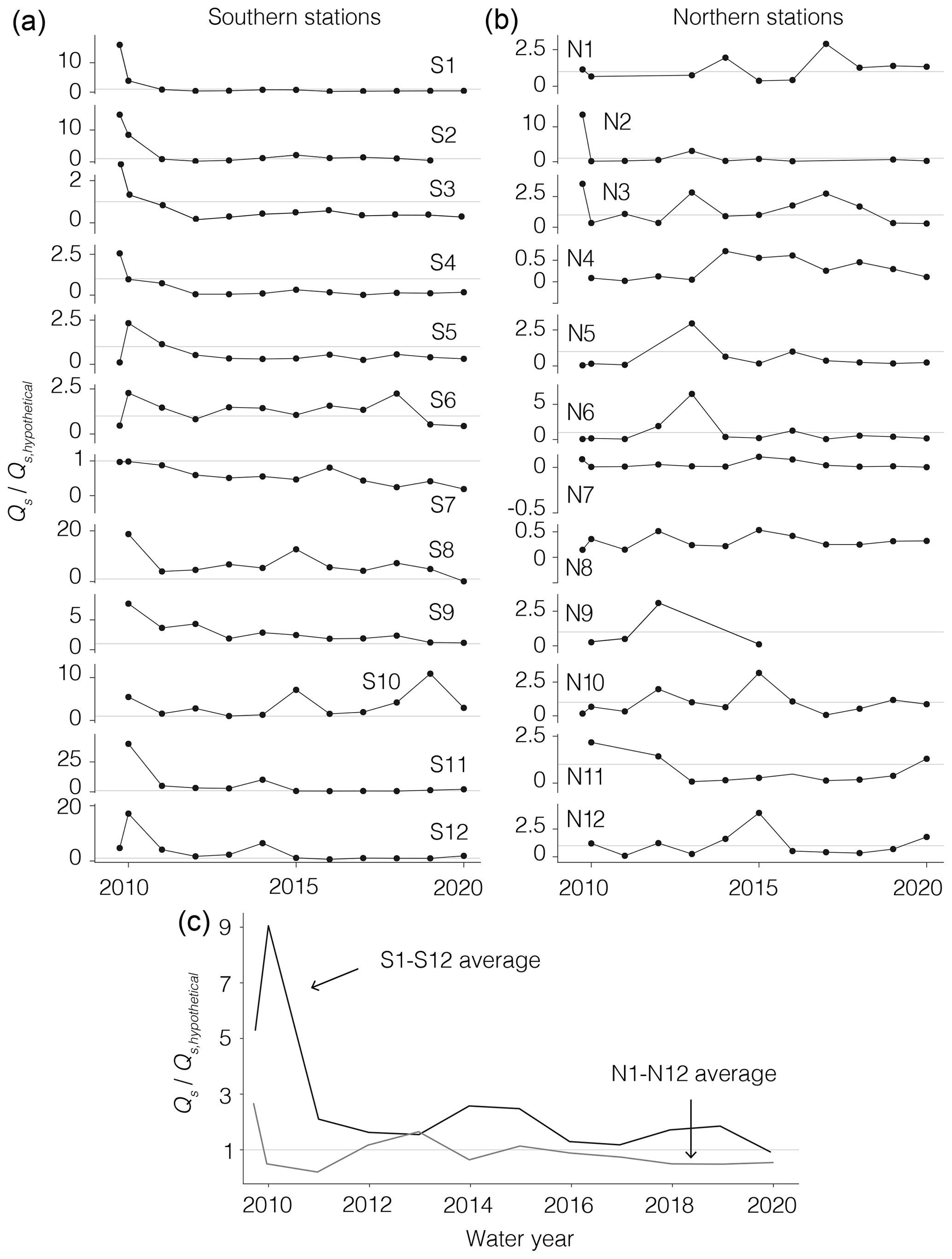
Figure 7 $Q_{\mathrm{s}}/Q_{\mathrm{s},\mathrm{hypothetical}}$ after Morakot at the focus gauging stations (Fig. 1). Horizontal gray lines indicate $Q_{\mathrm{s}}/Q_{\mathrm{s},\mathrm{hypothetical}}=\mathrm{1}$. Note the different y-axis extents in the individual station plots. At all but one of the southern focus stations, Q_s was elevated above Q_{s,hypothetical} at some point in the first 2 years after Morakot. By contrast, at 7 of the 12 northern stations, Q_s does not exceed Q_{s,hypothetical} at any time in the first 2 years after Morakot. The bottom panel shows the average $Q_{\mathrm{s}}/Q_{\mathrm{s},\mathrm{hypothetical}}$ ratios across the southern and northern focus stations. This shows that Q_s at the southern stations was, on average, substantially higher than Q_{s,hypothetical} in the first 2 years after Morakot, but not at the northern stations.

On average, Q_s tended to be substantially larger than Q_{s,hypothetical} across the southern stations for less than 2 years after Morakot (Fig. 7). Q_s exceeded Q_{s,hypothetical} at 9 of the 12 southern stations in the post-Morakot portion of the 2009 water year (all but S5–S7), 9 of the 12 stations in 2010 (all but S3, S4, and S7), and 10 of the 12 stations in 2011 (all but S4 and S7). On average across the southern stations, Q_s was 3.5 times higher than Q_{s,hypothetical} in the post-Morakot portion of 2009 and 9.1 times higher in 2010 (Fig. 7).

From 2011 onward, however, Q_s was only moderately larger than Q_{s,hypothetical} at the southern stations, and then only at some stations. Between 2012 and 2020, Q_s exceeded Q_{s,hypothetical} more than half the time at only 7 of the 12 southern stations. On average, Q_s was 0.8–2.6 times as large as Q_{s,hypothetical} across the southern stations from 2012 to 2020.

By contrast, at the northern stations, Q_s does not systematically exceed Q_{s,hypothetical} at any time in the decade after Morakot. In the post-Morakot portion of 2009, $Q_{\mathrm{s}}/Q_{\mathrm{s},\mathrm{hypothetical}}$ ratios are 13 and 4 at stations N2 and N3, respectively, but are not significantly above 1 at any of the other northern stations. This reflects the absence of a strong suspended sediment response to Morakot at the northern stations, even in the few months immediately after Morakot.

How much extra sediment was mobilized in the study rivers in the decade after Morakot? To calculate this, we define a new term, ΔQ_s, as the difference between Q_s and Q_{s,hypothetical}. We integrated ΔQ_s over the time from Morakot through 2020 to obtain the excess mass of suspended sediment discharged at each station over this decade. To facilitate comparisons to landslide intensity, we divided ΔQ_s by drainage area (A) and bedrock density ρ_r and termed this the excess sediment yield (Fig. 8) to ensure that this and I_L share the same dimensions of volume per area.

Figure 8 Excess suspended sediment yield ($\mathrm{\Delta }{Q}_{\mathrm{s}}=Q_{\mathrm{s}}-Q_{\mathrm{s},\mathrm{hypothetical}}$) per unit drainage area A integrated over time Δt from Morakot through 2020 as a function of landslide intensity I_L for all stations with positive ΔQ_s and I_L values (n=24). Here, values of Q_s have been converted from mass fluxes to volume fluxes by dividing by a bedrock density ρ_r of 2700 kg m⁻³ to facilitate comparison to the units of I_L we use elsewhere in this study (m³ km⁻²). The log–log regression through these data (black line) has a slope of 0.394±0.110, implying that excess sediment yield tended to be larger in basins with more intense Morakot-induced landsliding. Colors represent the average upstream precipitation during Morakot, which correlate broadly with landslide intensity (see also Fig. S3) and suggest that we cannot rule out an additional source of sediment driven by heavy precipitation besides landslides.

Figure 8 plots the excess sediment yield against I_L. The slope of the best-fit log–log regression is 0.394±0.110, showing that the excess sediment yield tended to be larger in basins with more intense landsliding. The excess sediment yield is larger than I_L for 68 % of the stations (data points above the 1:1 line in Fig. 8). These are generally restricted to stations with low landslide intensity, with none at I_L > 10⁵ m³ km⁻². This implies that landslide-derived material was not the source of all of the excess suspended sediment discharged from these rivers in the decade after Morakot. Meanwhile, the excess sediment yield was smaller than I_L for the remaining 32 % of the stations, all of which were in basins with high landslide intensity (I_L > 10⁴ m³ km⁻²). In these rivers, by contrast, the volume of landslide-mobilized material was large enough to have supplied all the excess sediment yield.

Where would the excess sediment come from if not from landslides? We hypothesize that a large amount of additional sediment beyond that moved by Morakot-induced landslides was mobilized in the aftermath of Morakot. This is also evident in the slope of the regression in Fig. 8, which does not follow a direct 1:1 relationship with landslide intensity. In other words, although basins with greater I_L tend to have greater $\mathrm{\Delta }{Q}_{\mathrm{s}}/A$ values, basins with lower I_L experience a proportionally greater erosion rate relative to I_L than basins with larger I_L. In particular, roughly half of the basins with I_L > 10⁴ m³ km⁻² are below the 1:1 line, suggesting that a large proportion of the excess sediment could be landslide-driven in these basins. Meanwhile, for the basins on the opposite side of the 1:1 line, there must be some other source which we are unable to fully quantify.

4 Discussion

4.1 Duration of suspended sediment responses to Morakot

Many of the southern focus stations display a gradual decay in $\stackrel{\mathrm{̃}}{a}$ over time after Morakot (Fig. 9). In Fig. 9, we fit the post-Morakot decay of $\stackrel{\mathrm{̃}}{a}$ to a linear regression of ln($\stackrel{\mathrm{̃}}{a}$) against time, consistent with exponential decay. The mean and standard error of the regression slope quantify the rate and decay of $\stackrel{\mathrm{̃}}{a}$ and its uncertainty, and they are listed in the panels of Fig. 9. These regressions capture the reduction in $\stackrel{\mathrm{̃}}{a}$ well at 10 of the 12 southern stations, where the mean regression slope is larger than the standard error of the slope by an average factor of 4.5 (range 2.4–8.7). At the two remaining stations (S8 and S10), the regression slope is zero within uncertainty, implying no resolvable change in $\stackrel{\mathrm{̃}}{a}$ (Fig. 9).

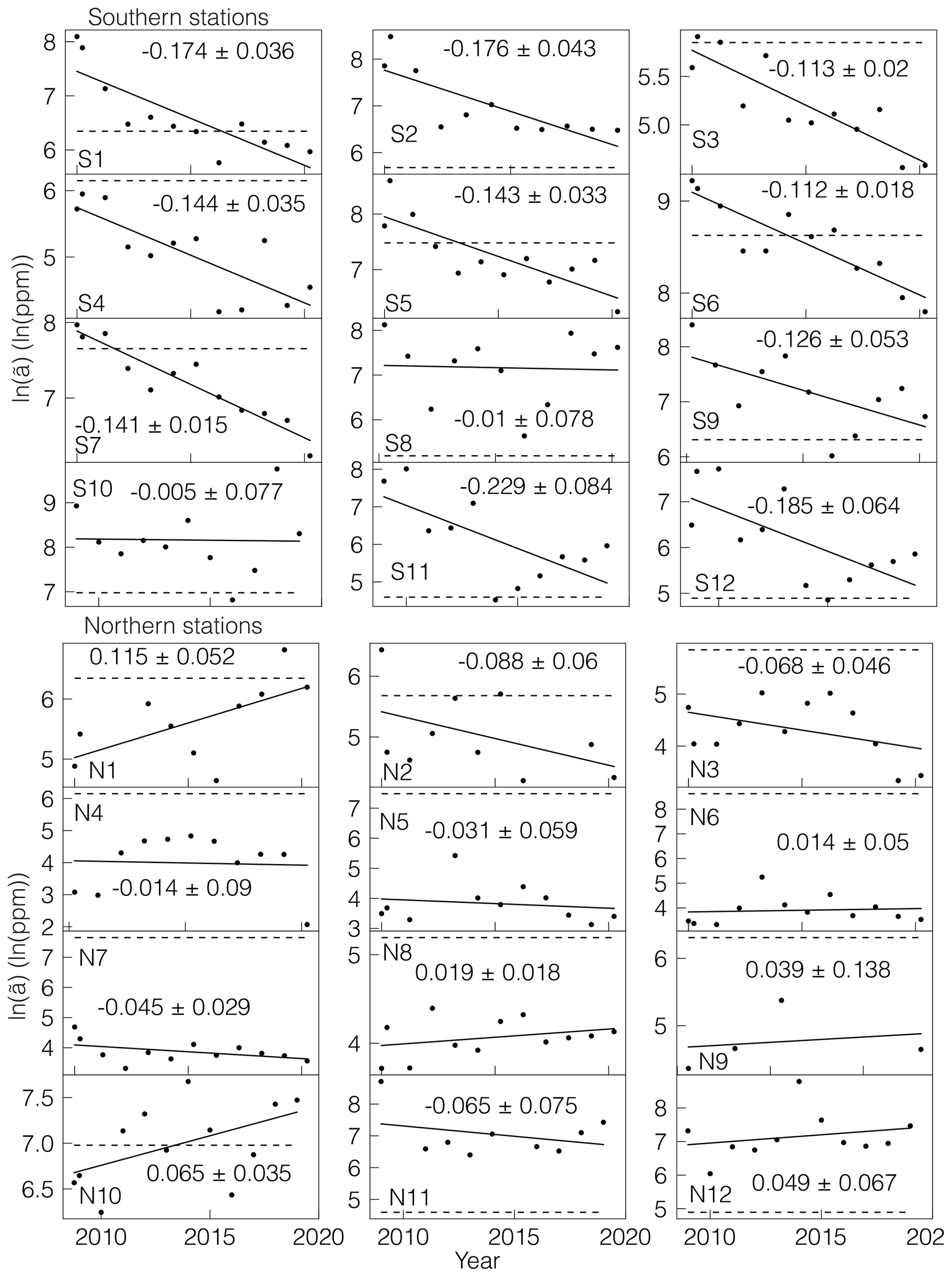
Figure 9 Solid lines are linear regressions of the rating curve parameter ln($\stackrel{\mathrm{̃}}{a}$) (black dots) with respect to time. Numbers in each panel are mean ± standard error of the slope of the regression line. A total of 10 of the 12 southern stations show a decreasing trend with time. In contrast, at the northern stations, regressions of ln($\stackrel{\mathrm{̃}}{a}$) against time have a range of positive and negative slopes with larger uncertainties. This suggests that the effects of Morakot decayed over time at most of the southern stations but not the northern stations. Dashed lines indicate values of the rating curve coefficient before Morakot.

By contrast, regressions of ln($\stackrel{\mathrm{̃}}{a}$) over time fit the data poorly at the northern stations. Regression slopes are indistinguishable from zero within 1 standard error uncertainty at 6 of the 12 stations (N4–N6, N8, N11, N12), positive at 3 stations (N1, N9, N10), and negative at the remaining 3 stations (N2, N3, N7; Fig. 9). At none of the three stations with negative regression slopes does the mean regression slope exceed 2 times the regression slope's standard error. This shows that post-Morakot trends in $\stackrel{\mathrm{̃}}{a}$ did not vary systematically across the northern stations and that at the few stations at which $\stackrel{\mathrm{̃}}{a}$ did decline, the decline is less clear than it is at the southern stations.

How long did the Morakot-induced perturbations to $\stackrel{\mathrm{̃}}{a}$ last? To answer this question, we introduce the notation ${\mathit{\tau }}_{\stackrel{\mathrm{̃}}{a}}$ to denote the characteristic response time of $\stackrel{\mathrm{̃}}{a}$. In Fig. 9, the linear regressions of ln($\stackrel{\mathrm{̃}}{a}$) vs. time describe exponential decay of $\stackrel{\mathrm{̃}}{a}$, which makes it convenient to define ${\mathit{\tau }}_{\stackrel{\mathrm{̃}}{a}}$ as the negative reciprocal of the regression slope (i.e., $\stackrel{\mathrm{̃}}{a}\left(t\right)\propto e^{-t/{\mathit{\tau }}_{\stackrel{\mathrm{̃}}{a}}}$). Stations with rapid declines in $\stackrel{\mathrm{̃}}{a}$ after Morakot have large regression slopes and hence small values of ${\mathit{\tau }}_{\stackrel{\mathrm{̃}}{a}}$ (short response times), while stations with slow declines in $\stackrel{\mathrm{̃}}{a}$ have small regression slopes and large values of ${\mathit{\tau }}_{\stackrel{\mathrm{̃}}{a}}$ (long response times). Under this definition, ${\mathit{\tau }}_{\stackrel{\mathrm{̃}}{a}}$ ranges from 4.4 ($+\mathrm{2.5}/-\mathrm{1.2}$) years to 9.0 ($+\mathrm{1.7}/-\mathrm{1.3}$) years at the 10 southern stations that have declining values of $\stackrel{\mathrm{̃}}{a}$ after Morakot. A property of exponential decay is a return to values within 5 % of background after roughly three characteristic decay times, so a return to near-background values at these stations would occur after 2 to 3 decades. At the remaining two stations (S8 and S10), the regression slopes are indistinguishable from zero within 1 standard error, implying values of ${\mathit{\tau }}_{\stackrel{\mathrm{̃}}{a}}$ indistinguishable from infinity. Uncertainties in ${\mathit{\tau }}_{\stackrel{\mathrm{̃}}{a}}$ are calculated as the negative reciprocals of the 1 standard error uncertainty bounds on the regression slopes in Fig. 9 (Table S2). Figure 9 shows that $\stackrel{\mathrm{̃}}{a}$ declines to values approaching ${\stackrel{\mathrm{̃}}{a}}_{\mathrm{pre}}$ within the 11-year time frame at four of the southern focus stations, and it declines to values below ${\stackrel{\mathrm{̃}}{a}}_{\mathrm{pre}}$ at six of the southern focus stations.

To quantify the post-Morakot changes in $\stackrel{\mathrm{̃}}{a}$ in rivers across Taiwan, we calculated regression slopes of ln($\stackrel{\mathrm{̃}}{a}$) vs. time for all stations with landslide intensities greater than 1 m³ km⁻² and with sufficient observations to compute post-Morakot trends (n=40; Table S2). We also calculated ${\mathit{\tau }}_{\stackrel{\mathrm{̃}}{a}}$ for the 26 stations at which a declines after Morakot to obtain characteristic decay times. The remaining 14 stations have positive regression slopes, indicating a post-Morakot increase in $\stackrel{\mathrm{̃}}{a}$. Figure 10a reveals that, in the 25 basins with relatively high landslide intensities (I_L > 1000 m³ km⁻²), regression slopes tend to be more negative at higher landslide intensity. Moreover, among these 25 high-I_L basins, only 3 have positive regression slopes, while 16 have negative regression slopes and the remaining 6 have regression slopes indistinguishable from zero. This reflects both the tendency of a to decay more rapidly in high-I_L basins and the variability in decay rates of a among basins, such as that exhibited by the difference between stations S8 and S10 (which have regression slopes indistinguishable from zero; Fig. 9) and the other 10 southern focus stations, which all have negative regression slopes. By contrast, in the 15 basins with relatively low landslide intensities (I_L < 1000 m³ km⁻²), regression slopes tend to be close to zero or slightly positive and uncorrelated with landslide intensity. Only 4 of these 15 low-I_L basins have negative regression slopes, while the remaining 11 have regression slopes that are positive or indistinguishable from zero. Similarly, Fig. 10b shows that ${\mathit{\tau }}_{\stackrel{\mathrm{̃}}{a}}$ tends to be shorter at larger values of I_L. For instance, the mean and standard error of ${\mathit{\tau }}_{\stackrel{\mathrm{̃}}{a}}$ are 5.8 ± 0.3 years in the basins with the largest landslide intensities (I_L > 10⁵ m³ km⁻²) and 36.4 ± 14.5 years at landslide intensities smaller than that. This indicates faster fractional responses of $\stackrel{\mathrm{̃}}{a}$ in basins that were hit harder by landsliding.

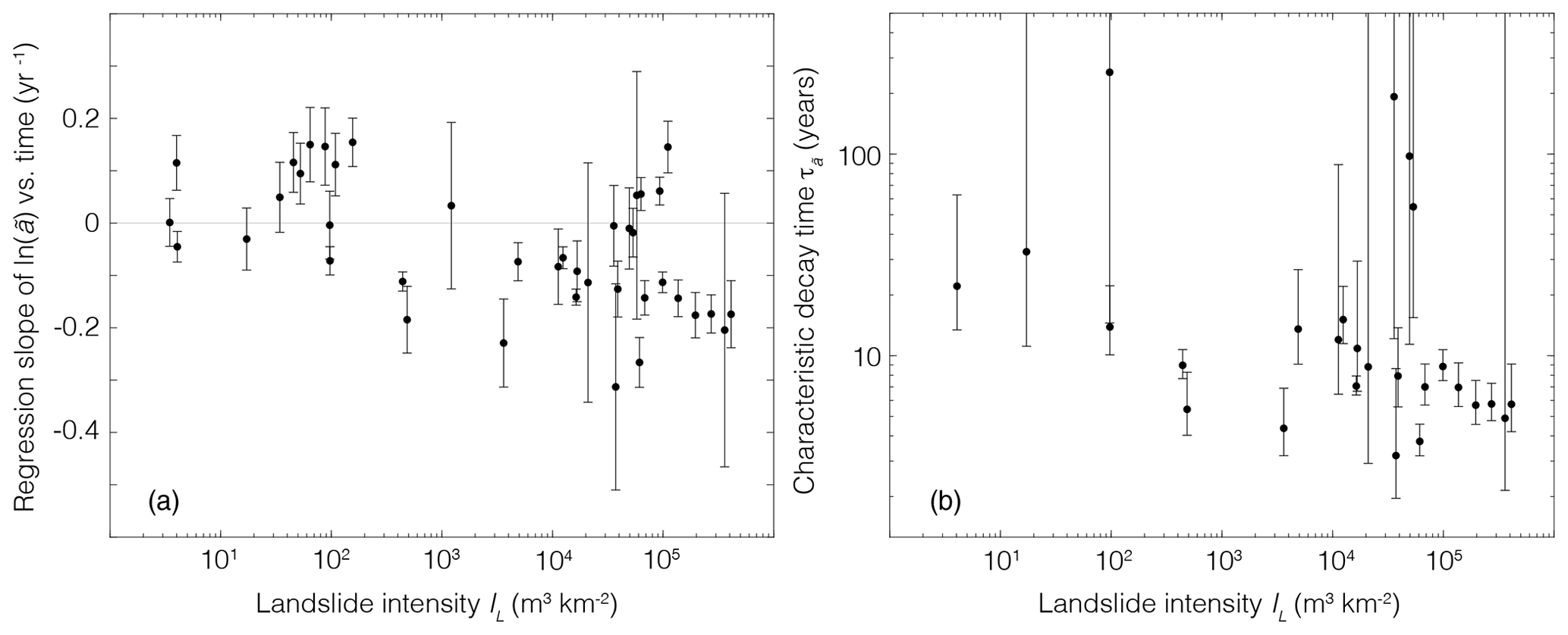
Figure 10 (a) Means and standard errors of the slopes of the log₁₀($\stackrel{\mathrm{̃}}{a}$) vs. time regressions (Fig. 9) for the 40 basins with nonzero landslide intensity. A total of 26 of the 40 regression slopes are negative, indicating decay of $\stackrel{\mathrm{̃}}{a}$ over time, and the remaining 14 are positive, indicating growth. (b) Characteristic decay times of $\stackrel{\mathrm{̃}}{a}$ for the stations with negative regression slopes, calculated as the negative reciprocal of values in Fig. 10a. Values of ${\mathit{\tau }}_{\stackrel{\mathrm{̃}}{a}}$ tend to be smaller at higher I_L values, implying that the elevated efficiency of suspended sediment transport after Morakot decayed more quickly in basins hit harder by landslides.

Together, Figs. 9–10 suggest that sediment transport was more efficient (i.e., $\stackrel{\mathrm{̃}}{a}$ was higher) after Typhoon Morakot than it was before it but that this elevated efficiency should only persist for a geologically short time (no longer than a few decades) and only in basins with abundant landslides. This implies that large landslide deposits in these rivers should persist for long times. This is consistent with Chen et al. (2020), who observed that ¹⁰Be concentrations in stream sediment were lower in 2016 than they were before Morakot in some rivers and higher in other rivers. This can be interpreted as an indication that, in some rivers, the Morakot-derived pulse of sediment had not yet been transported away by 2016, while in other rivers it had. The results are also consistent with DeLisle et al. (2022), who observed channel sediment aggradation of tens of meters in the steep upper reaches of catchments in southern Taiwan and who suggested that this sediment may take several centuries to excavate in some channels. Such a protracted duration of landslide sediment export may reflect the large volume and coarse grain size of landslide-derived sediment relative to the river's transport capacity, at least for basins with intense landsliding (Yanites et al., 2010; DeLisle et al., 2022; Marc et al., 2021).

4.2 Influence of landslide intensity on rating curves

How much did the intensity of landsliding affect the magnitude of the responses in the rating curve parameters? Here we examine the sensitivity of the Morakot-induced changes in the rating curve parameters to basin-averaged landslide intensity. To facilitate this comparison, we define $\mathrm{\Delta }{\log }_{\mathrm{10}}\left(\stackrel{\mathrm{̃}}{a}\right)$ as the change in log₁₀$\left(\stackrel{\mathrm{̃}}{a}\right)$ from before Morakot to a given time after it.

$$\begin{array}{}\text{(8)}& \mathrm{\Delta }{\log }_{\mathrm{10}}\left(\stackrel{\mathrm{̃}}{a}\right)={\log }_{\mathrm{10}}\left({\stackrel{\mathrm{̃}}{a}}_{\mathrm{post}}\right)-{\log }_{\mathrm{10}}\left({\stackrel{\mathrm{̃}}{a}}_{\mathrm{pre}}\right)\end{array}$$

Here ${\stackrel{\mathrm{̃}}{a}}_{\mathrm{post}}$ is the value of $\stackrel{\mathrm{̃}}{a}$ in the post-Morakot period of interest and ${\stackrel{\mathrm{̃}}{a}}_{\mathrm{pre}}$ is the average value of $\stackrel{\mathrm{̃}}{a}$ during the monitoring period before Morakot, as defined in Sect. 2.1. For example, if we denote ${\stackrel{\mathrm{̃}}{a}}_{\mathrm{2009}\mathrm{PM}}$ to be the value of $\stackrel{\mathrm{̃}}{a}$ in the post-Morakot portion of water year 2009, then $\mathrm{\Delta }{\log }_{\mathrm{10}}\left(\stackrel{\mathrm{̃}}{a}\right)={\log }_{\mathrm{10}}\left({\stackrel{\mathrm{̃}}{a}}_{\mathrm{2009}\mathrm{PM}}\right)-{\log }_{\mathrm{10}}\left({\stackrel{\mathrm{̃}}{a}}_{\mathrm{pre}}\right)$. We define Δb the same way in Eq. (9).

$$\begin{array}{}\text{(9)}& \mathrm{\Delta }b=b_{\mathrm{post}}-b_{\mathrm{pre}}\end{array}$$

Here b_post is the value of b in the post-Morakot period of interest and b_pre is the average value of b in the monitoring period before Morakot. Figure 11a plots $\mathrm{\Delta }{\log }_{\mathrm{10}}\left(\stackrel{\mathrm{̃}}{a}\right)$ against I_L for the post-Morakot portion of 2009 for all basins with nonzero I_L. Here, each data point represents a single gauging station. A linear regression through these data has a slope of 0.11±0.05 log₁₀(ppm)/log₁₀(m³ km⁻²), indicating that, during the first few months after Morakot, values of $\stackrel{\mathrm{̃}}{a}$ tended to increase more in basins that were hit harder by landsliding. Analogous figures for each year after Morakot are shown in Fig. S5.

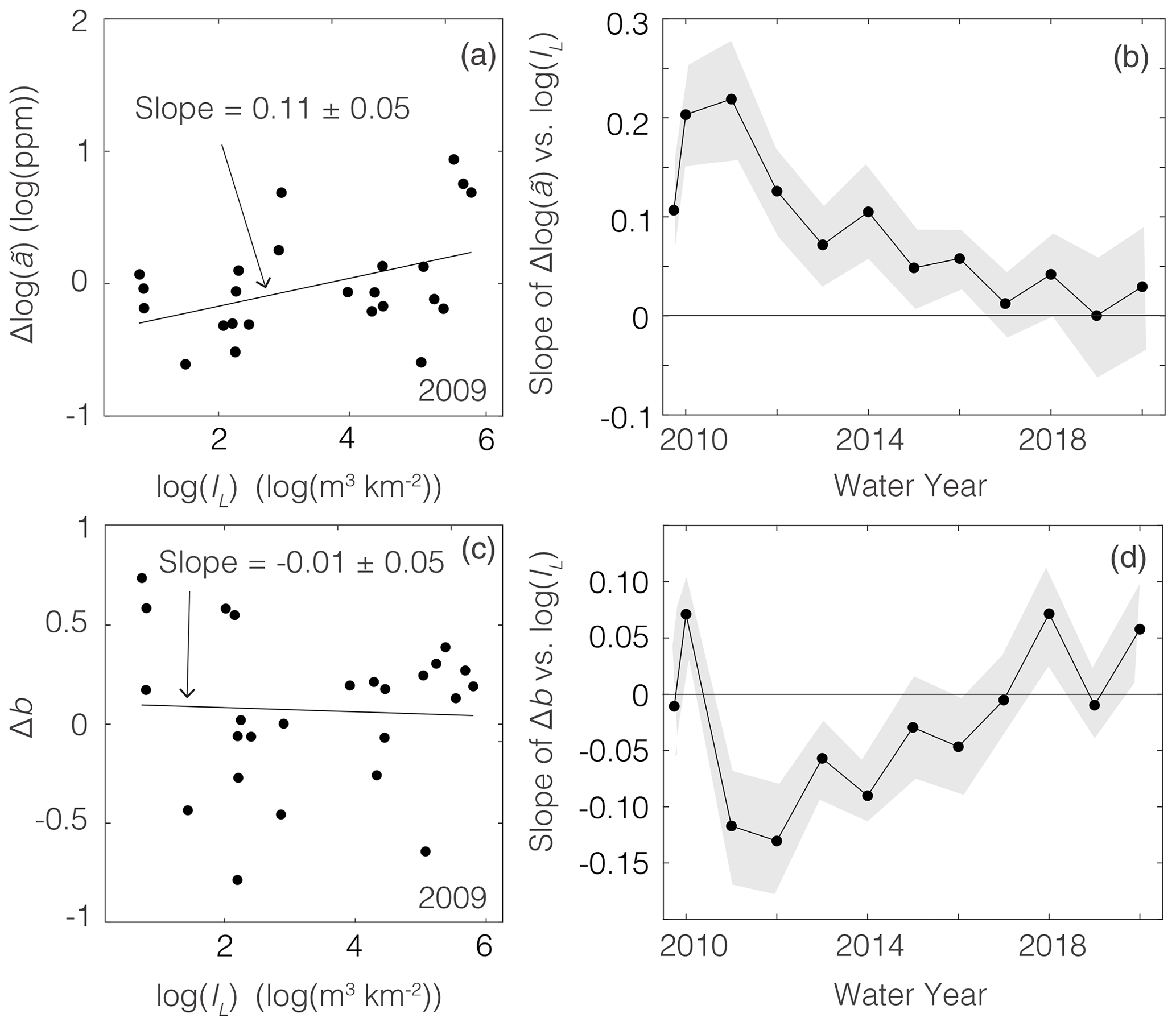
Figure 11 (a) Sensitivity of the rating curve coefficient $\stackrel{\mathrm{̃}}{a}$ to the basin-averaged intensity of Morakot-induced landslides I_L. Δlog ₁₀ ($\stackrel{\mathrm{̃}}{a}$) is the difference in log₁₀($\stackrel{\mathrm{̃}}{a}$) between a given time (in panel a, the post-Morakot portion of 2009) and the pre-Morakot value ${\stackrel{\mathrm{̃}}{a}}_{\mathrm{pre}}$. The regression line's positive slope shows that $\stackrel{\mathrm{̃}}{a}$ tended to increase more in basins that were hit harder by Morakot-induced landsliding. Analogous figures for other years after Morakot are shown in Fig. S5. (b) Annual means (dots and line) ± standard errors (shaded region) of regression slopes of Δlog ₁₀ ($\stackrel{\mathrm{̃}}{a}$) against log₁₀(I_L) for each year after Morakot, computed as in panel (a). The slope between Δlog ₁₀ ($\stackrel{\mathrm{̃}}{a}$) and log ₁₀(I_L) gradually decreased over time, implying that the sensitivity of $\stackrel{\mathrm{̃}}{a}$ to I_L was no longer apparent by ∼ 7 years after Morakot. (c) As in panel (a), except showing the change in b relative to the pre-Morakot value b_pre. The regression slope is indistinguishable from zero within error, indicating that b was insensitive to the intensity of Morakot-induced landsliding during this time. Analogous figures for other years are shown in Fig. S6. (d) Changes in b were positively correlated with I_L in 2010, then negatively correlated for several years in a row. This is consistent with a weak sensitivity of b to the intensity of landsliding for 4 years after Morakot.

Figure 11b shows that the slope between $\mathrm{\Delta }{\log }_{\mathrm{10}}\left(\stackrel{\mathrm{̃}}{a}\right)$ and basin-averaged I_L gradually decreased over time. The strength of the positive correlation between $\mathrm{\Delta }{\log }_{\mathrm{10}}\left(\stackrel{\mathrm{̃}}{a}\right)$ and I_L peaked at 0.22±0.06 log₁₀(ppm)/log₁₀(m³ km⁻²) in 2011 and gradually grew weaker for several years after that. From 2017 onward, the mean regression slope of the correlation was indistinguishable from zero within 1 standard error. Thus, the correlation between increases in $\stackrel{\mathrm{̃}}{a}$ and landslide intensity persisted for roughly 6 years after Morakot.

Figure 11c plots Δb against I_L for the post-Morakot portion of 2009. As in Fig. 11a, each data point represents a single gauging station. A linear regression through these data has a slope of $-\mathrm{0.01}\pm \mathrm{0.05}$ (log₁₀(m³ km⁻²))⁻¹, indicating that, during the first few months after Morakot, values of b were insensitive to the intensity of landsliding. Analogous figures for each year after Morakot are shown in Fig. S6.

Figure 11d shows the complex relationship between Δb and I_L over time. This relationship was positive in the post-Morakot portion of water year 2009 and in 2010, indicating a brief period in which b values were positively correlated with landslide intensity. Then, in 2011, they became negatively correlated and remained so for several years. The strength of the negative correlation peaked at $-\mathrm{0.13}\pm \mathrm{0.05}$ (log₁₀(m³ km⁻²))⁻¹ in 2012 and gradually grew weaker for several years after that. By 2015, the mean regression slope was indistinguishable from zero within 1 standard error. Thus, the negative correlation between Δb and landslide intensity persisted for roughly 4 years from 2011 to 2014.

Together, the results in Fig. 11 imply that the sensitivity of rating curve parameters to landslide intensity is resolvable in this group of gauging stations for 4–6 years after Morakot and slightly longer for log₁₀$\left(\stackrel{\mathrm{̃}}{a}\right)$ than b. This is comparable to the average duration of elevated values of $\left(\stackrel{\mathrm{̃}}{a}\right)$ and lowered values of b (Fig. 4). Beyond that time, there is no discernible influence of Morakot-induced landslide intensity on changes in log₁₀$\left(\stackrel{\mathrm{̃}}{a}\right)$ and b. This is consistent with a persistent, decaying influence of sediment supply changes on the rating curve parameters over roughly half a decade.

4.3 Potential drivers of post-Morakot variations in rating curves

As described in Sect. 3.1, estimates of $\stackrel{\mathrm{̃}}{a}$ increased immediately after Morakot at 11 of the 12 southern stations (all but S6). What was responsible for this systematic increase? Huang and Montgomery (2013) noted that a shift from coarser to finer suspended sediment would generate a decrease in b at the same time as an increase in $\stackrel{\mathrm{̃}}{a}$, which they used to explain the coincident increase in $\stackrel{\mathrm{̃}}{a}$ and decrease in b at 15 of the 19 gauging stations they analyzed in the first 2 years after Morakot (2009–2011). This interpretation was supported by bed grain size measurements made by Taiwan's Water Resources Agency at one station in the Beinan River, which revealed a reduction in median grain size after Morakot (Huang and Montgomery, 2013).

We are unaware of pre-Morakot and post-Morakot grain size measurements at other stations, but if Morakot induced a reduction in grain size at all the study rivers, then this would explain the systematic increase in $\stackrel{\mathrm{̃}}{a}$ immediately after Morakot. It also implies that b should have decreased at the same time that $\stackrel{\mathrm{̃}}{a}$ increased. Contrary to this expectation, however, b was lower than b_pre in 2009 and 2010 at fewer than half of the stations at which $\stackrel{\mathrm{̃}}{a}$ exceeded ${\stackrel{\mathrm{̃}}{a}}_{\mathrm{pre}}$. In the post-Morakot portion of 2009, b was lower than b_pre at only two of the seven southern stations with sufficient measurements (S5 and S7; Tables S2 and S4). At the other five stations (S1–S4 and S12), b increased during this time rather than decreasing. In 2010, b was lower than b_pre at 5 of the 11 stations at which $\stackrel{\mathrm{̃}}{a}$ exceeded ${\stackrel{\mathrm{̃}}{a}}_{\mathrm{pre}}$ (S1, S2, S5, S7, and S10), but b was higher than b_pre at the other 6. This brief period of elevated b values in 2010 was followed by 3–6 years in which b values were, on average, lower than pre-Morakot values. Thus, across the southern study basins, where landsliding was prevalent, the systematic reduction in b values occurred in 2011, roughly 1.3 years after Morakot and the increase in $\stackrel{\mathrm{̃}}{a}$ values. To the extent that the reduction in b reflects a shift from threshold bed to live bed sediment transport (Huang and Montgomery, 2013), this suggests a brief period of adjustment toward these conditions after Morakot.

Could other events, like additional typhoons, have affected estimates of the rating curve parameters after Morakot? At many of the southern stations, there is considerable interannual variation in $\stackrel{\mathrm{̃}}{a}$ around the downward trend after Morakot, which is reflected in the uncertainties in the regression slopes in Fig. 9. Typhoon Fanapi, for example, brought intense rainfall to southern Taiwan in September 2010, and the estimates of $\stackrel{\mathrm{̃}}{a}$ at most of the southern focus stations in 2010 lie above the regression slopes in Fig. 9. Could Fanapi have introduced more landslide-derived sediment to the study rivers than Morakot did?

The fluvial water discharge measurements suggest this is unlikely. At the Beinan River station that is farthest downstream (WRA station 1730 H043; Table S1), the maximum average daily discharge during Typhoon Fanapi was 2800 m³ s⁻¹, roughly 15 % of the maximum discharge during Morakot (nearly 15 000 m³ s⁻¹). To the extent that landslide occurrence is correlated with river discharge, this suggests that Fanapi may have contributed to elevated values of $\stackrel{\mathrm{̃}}{a}$ in 2010 but that the responses in $\stackrel{\mathrm{̃}}{a}$ to Fanapi were likely smaller than the responses to Morakot. It is possible, however, that in addition to contributing landslide sediment after Morakot, runoff from Fanapi (the first major typhoon of the 2010 season to hit the Beinan basin) may have introduced additional sediment from Morakot-induced landslides to the fluvial network in the same way that Typhoon Toraji did in 2001 after the 1999 Chi-Chi earthquake (e.g., Dadson et al., 2003). This is supported by the study of Hung et al. (2018), which showed that the destabilizing effects from Morakot may have contributed to increased landslide intensity for ∼ 5 years after the typhoon. Teng et al. (2020) also demonstrate through numerical modeling that reactivated, old landslide material can influence sediment transport after a large landsliding event.

A counterexample is Typhoon Soulik, which was the largest typhoon to hit Taiwan in 2013, the most active typhoon season in Taiwan since 2004. Soulik produced heavy rainfall on both the north and south sides of the island, peaking at > 600 mm on 13 July (Wu et al., 2018). This coincided with a small peak in $\stackrel{\mathrm{̃}}{a}$ in 2013 at some stations on the northwest side of the island (N1–N6) but relatively small responses at the remaining northern stations and most southern stations (Figs. 4, 9). Among the southern stations, only S3 shows a local maximum in $\stackrel{\mathrm{̃}}{a}$ during 2013, when $\stackrel{\mathrm{̃}}{a}$ was 68 % higher than in 2012. This suggests that Soulik had a relatively small effect on suspended sediment transport in most of the study rivers, unlike Morakot, underlining the fact that the Morakot-induced increases in sediment fluxes were likely due to the combined effects of intense landsliding and flooding rather than flooding alone. Furthermore, at many stations, the largest recorded flood event during 1990–present occurred in years other than 2009 (white stars, Fig. 4; Fig. S2). This suggests that Morakot-induced changes in $\stackrel{\mathrm{̃}}{a}$ and b were likely driven by changes in landslide-derived sediment supply, not changes in Q.

A final potential driver of post-Morakot changes in a and b relates to the channel itself. If the channel cross-sectional geometry changed during Morakot (e.g., through widening or deepening), then a given Q could generate a different basal shear stress after Morakot than before it, which in turn could generate a different relationship between C and Q and hence different values of a and b. Identifying any such effects is beyond the scope of this study but may be useful in future studies to help interpret sediment discharge estimates at individual stations.

5 Conclusions

The primary contribution of this study is a new assessment of the effects of Typhoon Morakot on fluvial suspended sediment loads over an 11-year period after Morakot in 87 rivers around Taiwan. The most striking signal is a peak in the rating curve coefficient $\stackrel{\mathrm{̃}}{a}$ within 1 year of Morakot, with larger fractional increases in $\stackrel{\mathrm{̃}}{a}$ in basins with more intense landsliding. This was followed by a decline in $\stackrel{\mathrm{̃}}{a}$ with an exponential characteristic decay time of 3–255 years for all stations, with shorter (sub-decadal) decay times in basins with more intense landsliding (4–9 years for our southern focus stations). By contrast, the rating curve exponent b did not drop systematically until 2 years after Morakot, even in basins with abundant landsliding. The post-Morakot increases in $\stackrel{\mathrm{̃}}{a}$ and decreases in b tended to be larger in basins with more intense landsliding, but this sensitivity to landslide intensity decayed away within 4–7 years. In other words, while the decay times were similar for a and b, the response of a was uniform while b was not. These changes resulted in a positive correlation between excess suspended sediment yield and landslide intensity integrated over the decade after Morakot.

Together, these observations are consistent with an influence of landsliding on suspended sediment transport efficiency that was large immediately after Morakot and then diminished rapidly in most basins. This implies that in the basins that experienced the heaviest landsliding, the influence of Morakot-induced landsliding on suspended sediment concentrations substantially declined within the first decade after the typhoon and that its influence will disappear entirely within a few decades. To the extent that these results are applicable to other mountainous rivers, this suggests that rivers may be able to move landslide-derived sediment more efficiently for only a few years to decades after landslide events. Thus, although landslide deposits in river valleys may persist for centuries, elevated suspended sediment concentrations may only last a short fraction of that time.