the Creative Commons Attribution 4.0 License.
the Creative Commons Attribution 4.0 License.
 | 09 Jan 2024
Analysis of autogenic bifurcation processes resulting in river avulsion
Marco Redolfi
Marco Tubino
River bifurcations are constituent components of multi-thread fluvial systems, playing a crucial role in their morphodynamic evolution and the partitioning of water and sediment. Although many studies have been directed at exploring bifurcation dynamics, the conditions under which avulsions occur, resulting in the complete abandonment of one branch, are still not well understood. To address this knowledge gap, we develop a novel 1D numerical model based on existing nodal point relations for sediment partitioning, which allows for the simulation of the morphodynamic evolution of a free bifurcation. Model results show that when the discharge asymmetry is so high that the shoaling branch does not transport sediments (partial avulsion conditions) the dominant branch undergoes significant degradation, leading to a higher inlet step between the bifurcates and further amplifying the discharge asymmetry. The degree of asymmetry is found to increase with the length of the downstream channels to the point that when they are sufficiently long, the shoaling branch is completely abandoned (full avulsion conditions). To complement our numerical findings, we also formulate a new analytical model that is able to reproduce the essential characteristics of the partial avulsion equilibrium, which enables us to identify the key parameters that control the transition between different configurations. In summary, this research sheds light on the fundamental processes that drive avulsion through the abandonment of river bifurcations. The insights gained from this study provide a foundation for further investigations and may offer valuable information for the design of sustainable river restoration projects.
- Article
(3455 KB) - Full-text XML
- BibTeX
- EndNote


Bifurcations constitute essential geomorphic elements of a variety of fluvial systems, such as braiding rivers and deltas. The morphodynamic evolution of these systems strongly depends on the water and sediment partitioning set by the bifurcation node, which in turn is determined by the reach-scale morphodynamic processes occurring in the three branches connected by the bifurcation node. Understanding these processes is therefore key to foreseeing the behaviour of multi-thread systems across temporal scales, as well as designing sustainable river restoration projects (Habersack and Piégay, 2007).
Among the morphodynamic processes that occur at bifurcations, the partial or complete abandonment of one of the bifurcates is of crucial importance. This event, which leads to the diversion of the majority or all of the incoming water and sediment discharges towards one of the two bifurcates, can be considered one of the possible styles of river avulsions, such as “soft” or “choking” avulsions (Edmonds et al., 2011; Leddy et al., 1993). These processes have been shown to play a major role in the evolutionary trajectories of braiding networks (Ferguson, 1993), lowland rivers (Slingerland and Smith, 2004), river deltas (Salter et al., 2018), and alluvial fans (Field, 2001), as they can cause shifts in evolving morphologies and suddenly modify the flooding risk and water resource availability in the downstream areas. Moreover, a clear understanding of the conditions that can ensure the long-term preservation of bifurcating systems is also crucial for the effective implementation of river interventions aimed at recovering the eco-morphological quality of river ecosystems, thus reducing the need for intensive maintenance.
Although many studies have been directed at exploring the possible long-term states of bifurcations, little is known about the conditions for which avulsions occur during the transient stage of an evolving bifurcation. Among others, 1D approaches proved to be very effective in analysing the key mechanisms that govern water and sediment partitioning at bifurcation nodes. These studies stemmed largely from the analytical model developed by Bolla Pittaluga et al. (2003), hereafter referred to as BRT, where a quasi-2D physically based nodal relationship was used to describe the sediment partitioning at the node.
The BRT model was originally formulated to analyse the dependence on the parameters of the upstream flow of the long-term equilibrium states of a “free” bifurcation (i.e. in the absence of external factors influencing the morphodynamic processes occurring at the node). The model was further extended to include the effects of migrating bars (Bertoldi et al., 2009), tides (Ragno et al., 2020), curvature in the upstream channel (Kleinhans et al., 2012), slope advantage between the branches (Redolfi et al., 2019), and downstream effects generated by prograding branches (Salter et al., 2018).
The main outcome of the BRT model, later confirmed by the experimental results of Bertoldi and Tubino (2007), is the occurrence of two distinct regimes, depending on the values of the half-width to depth ratio β (hereafter referred to as “aspect ratio”) and the Shields stress θ of the upstream flow. Specifically, for low values of the aspect ratio β the model only admits one stable equilibrium solution, in which water and sediments are partitioned evenly by the bifurcation node; in other words, the only equilibrium state of the bifurcation is “balanced”. When the aspect ratio β exceeds a critical threshold, the balanced solution becomes unstable and the system admits two stable, anti-symmetric, and unbalanced equilibrium configurations. In these unbalanced equilibrium states, both branches are morphodynamically active; i.e. they have a non-negligible transport capacity. As highlighted by Redolfi et al. (2016), the critical aspect ratio is found to coincide with the resonant value that discriminates between prevailing upstream or downstream propagation of morphological changes (Zolezzi and Seminara, 2001), which reveals the close connection between the dynamics of free bifurcations and the framework of 2D morphodynamic influence.
However, when further increasing the value of β a second threshold appears, beyond which all stable equilibrium states identified by the BRT model are characterized by a branch with vanishing transport capacity (see Fig. 1). These states correspond to bifurcations in which one of the two branches is morphodynamically inactive and thus more likely to be abandoned as the bifurcation evolves. Under these conditions the theoretical predictions based on the BRT model are no longer suitable, as the model assumes that both branches are able to adjust their bed slope to a prescribed equilibrium value, which is clearly not possible for the channel that is no longer transporting sediments. The question then arises of whether in this condition the bifurcation can still attain an equilibrium state and to what extent such a state differs from that predicted by the BRT model. To address this question, an evolutionary model is required to trace the trajectory of a bifurcation starting from a nearly balanced initial state.
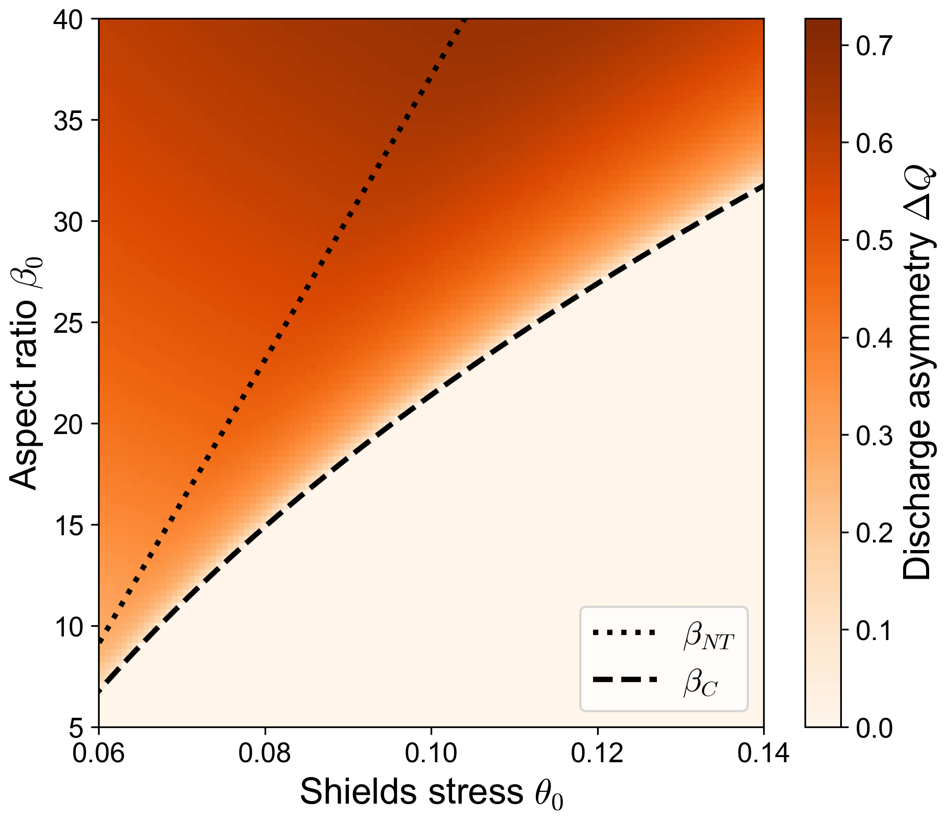
Figure 1Regions of the parameter space identifying different types of equilibrium solutions of river bifurcations computed by means of the BRT model (Bolla Pittaluga et al., 2003) for different combinations of the aspect ratio β0 and Shields stress θ0. The dashed line indicates the critical aspect ratio βC, which separates the region where the balanced equilibrium configuration is stable (lower right region of the plot) from the region where only unbalanced equilibrium configurations are stable (upper left portion of the plot). The dotted line indicates the no-transport aspect ratio βNT: when β0≥βNT, the BRT model predicts a vanishing transport capacity in the shoaling branch. Darker shades indicate larger values of the equilibrium discharge asymmetry ΔQ, defined as the difference in the water discharges flowing in the bifurcates, scaled by the incoming discharge.
In the past 2 decades, many authors have attempted to investigate the transient behaviour of bifurcations belonging to different fluvial environments, though most of these studies were focused on the effect of external forcing factors. For example, Salter et al. (2018) developed a numerical model to study the transient behaviour of bifurcations with prograding branches, considering suitable initial and boundary conditions for reproducing the evolutionary trajectories of bifurcations in depositional environments. Using a similar approach, Iwantoro et al. (2022) studied the effect of tides on the stability of bifurcations by properly varying the downstream boundary conditions. Other evolutionary models of bifurcations available in the literature were tailored to specific case studies, such as bifurcations located downstream of a reservoir (Mendoza et al., 2022) and longitudinal training walls in the presence of alternate bars in the upstream channel (Le et al., 2018).
The stability of equilibrium states of free bifurcations was indeed studied by Edmonds and Slingerland (2008). However, their analysis was limited to specific deltaic environments in which both branches of the bifurcation were always morphodynamically active. On the contrary, in some of the 3D numerical simulations performed by Kleinhans et al. (2008) all the incoming solid discharge was steered towards one of the two downstream branches. Analysing these simulations, the authors highlighted the limited capability of the BRT model – both in the original version and with the modifications proposed in their study – to correctly predict the equilibrium value of the water discharge asymmetry of the bifurcation. They specifically showed that bifurcations can display a much higher degree of asymmetry than that foreseen by BRT. Although the simulations considered a bifurcation with a curved upstream channel, thus introducing an external forcing in the model, this study highlighted the important role that the transient behaviour may have in determining the long-term equilibrium state of a bifurcation.
There is therefore a lack of knowledge about the transient behaviour of a free bifurcation and about the possible existence of an autogenic mechanism that may lead to the partial or complete abandonment of a branch. In this work, we aim to analyse the transient behaviour of an initially balanced bifurcation that spontaneously evolves over time. To this purpose, we employ a novel 1D numerical model that relies on the BRT relationship for sediment partitioning at the bifurcation node and accounts for the morphodynamic evolution of the three branches composing the bifurcation. By analysing the model outputs, we firstly outline the evolutionary processes that lead the system to reach its long-term, unbalanced equilibrium configuration. Secondly, we show how model results vary considerably according to the aforementioned regions of the BRT model parameter space, displayed in Fig. 1. Specifically, we show how the bifurcation may evolve towards considerably more unbalanced equilibrium states than those foreseen by the BRT model, including those in which one branch is completely abandoned. Lastly, we formulate a simple analytical model to characterize this new category of equilibrium states.
2.1 Formulation
We consider a free bifurcation consisting of three branches, each characterized by a rectangular cross-section and fixed banks. The widths of the bifurcates b and c are assumed to be both equal to half the width of the upstream branch a. The upstream channel is fed by constant liquid (Q0) and solid (Qs0) discharges, while at the outlet of the downstream branches b and c a constant water surface elevation hd is set. At the bifurcation node we also impose the water discharge balance and an equal water level for the three branches. Lastly, we employ the quasi-2D two-cell nodal condition proposed by Bolla Pittaluga et al. (2003) to compute the transverse exchange of sediments at the node.
To model the morphodynamic evolution of the bifurcation over time, we numerically solve the gradually varied flow equation and the Exner equation along the three branches according to a quasi-steady approach. As initial conditions we consider a balanced bifurcation, where water and sediments are partitioned equally among the downstream branches. After applying a small perturbation on the transverse bed slope between the branches, we then let the bifurcation evolve spontaneously over time.
2.1.1 Computation of hydrodynamic conditions and morphological evolution along the branches
The hydrodynamic conditions are evaluated by assuming that riverbed changes are much slower than flow adaptation, which implies that the solution for the liquid phase can be decoupled from that of the solid phase. The constancy of the water supply then implies that a unique value of water discharge can be considered for each branch. The water surface profile computation along each branch is then performed by integrating in the x direction the gradually varied flow equation:
where D is the water depth, S is the local bed slope, j is the energy gradient, and Fr is the Froude number. Both j and Fr are computed as functions of the water discharge Q and of the water depth D as
where W is the width of the branch, g is the gravity acceleration and C is the dimensionless Chézy coefficient, which for simplicity is considered here to be independent of the water depth and known a priori.
Integrating Eq. (1) along the downstream bifurcates requires knowledge of the respective flow rates, which we compute by means of an iterative procedure that relies on the assumption of equal surface elevation at the bifurcation node. This procedure is similar to that employed by previous models (e.g. Kleinhans et al., 2008) and will be described later in this section.
Once the water discharge and the water depth along the three branches have been determined, the evolution over time of the bed profile is computed by integrating in time the Exner equation, which for channels having a rectangular cross-section and constant width is written in the form
where t is the time, η the local bed elevation, p the bed porosity, and Qs the sediment flux. The latter is expressed as
where Δ is the relative submerged weight of sediments, Ds is the median grain size, and Φ(θ) is the dimensionless transport capacity per unit width. The latter is evaluated by means of a suitable transport formula (e.g. Meyer-Peter and Müller, 1948; Parker, 1978) as a function of the Shields stress θ, defined as
2.1.2 Water surface gradient and transverse solid discharge at the node cells
Following the approach proposed by Bolla Pittaluga et al. (2003), we model the last reach of the upstream channel a by means of two node cells, which are allowed to exchange water and sediments in the transverse direction. The length of the node cells is estimated as αWa, where α is an order-1 parameter for which different values have been proposed in the literature, as discussed by Redolfi (2023). For these node cells, the mathematical formulation must be amended to suitably represent the quasi-2D scheme introduced by BRT to account for the sediment transport redistribution driven by flow exchange and transverse bed slope.
The first question that arises is how to schematize the elevation gap between the two cells. Here we integrate the gradually varied flow equation and the Exner equation by considering the “triangular step” scheme represented in Fig. 2, i.e. by assuming that the bed elevation varies linearly along each node cell.
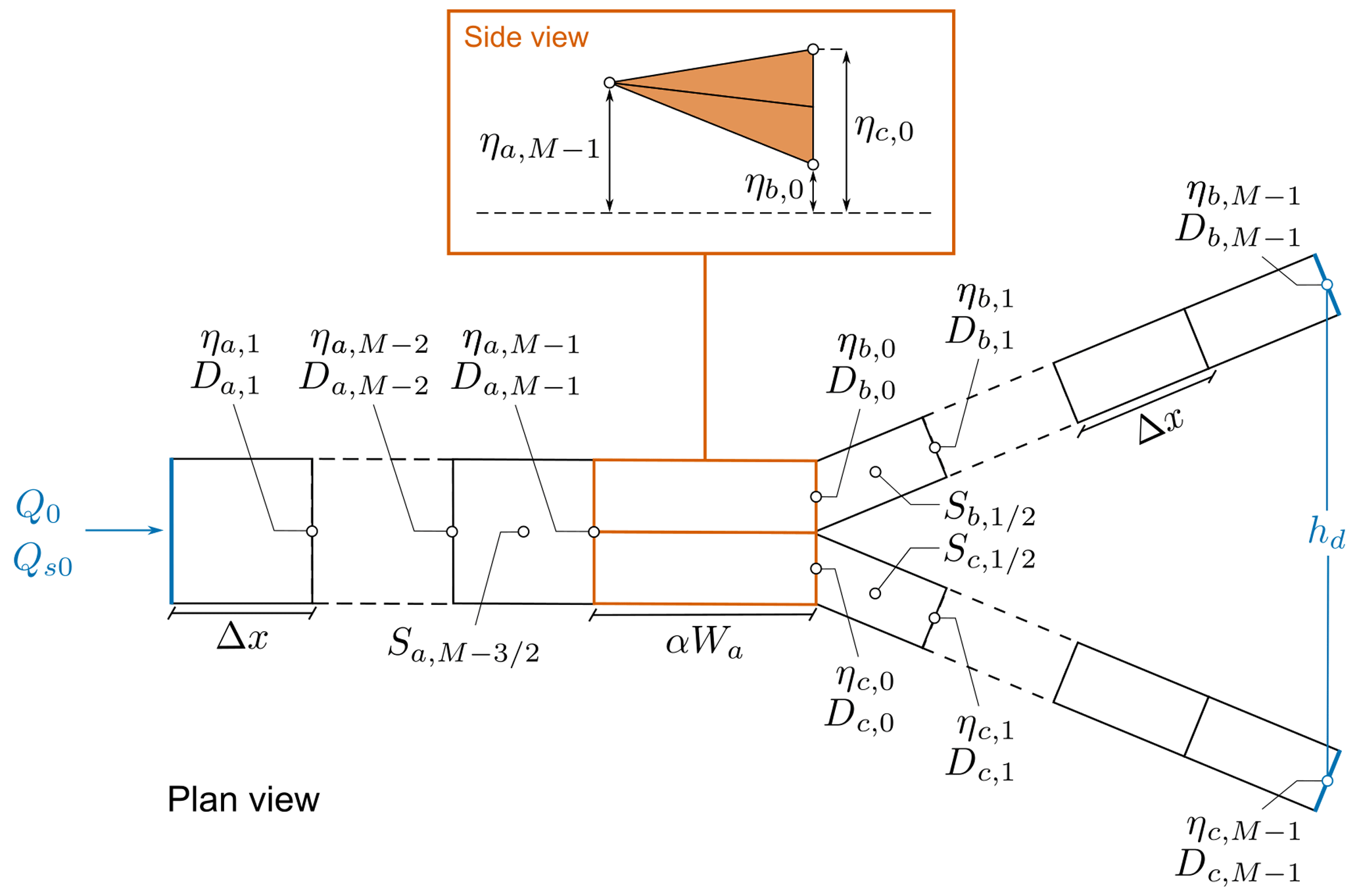
Figure 2Spatial discretization of water depth D, bed elevation η, and bed slope S along the channels and within the nodal bifurcation cells. The side view illustrates the triangular step scheme adopted for the bed elevation profiles of the node cells in detail, whose length is given by the product of the order-1 parameter α and the upstream channel width Wa. Q0 and Qs0 represent the water and sediment supply, while hd stands for the fixed water level at the downstream end of branches b and c.
A second issue concerns how the water surface profile is computed, specifically how to determine the water level at the inlet of the nodal cells, which sets the boundary condition for the computation of the backwater profile along the upstream channel a. Most existing 1D models (e.g. Kleinhans et al., 2008; Iwantoro et al., 2022) solve this problem by assuming a constant water surface elevation throughout the bifurcation cells. However, considering that the nodal cells extend over several channel width, this may be not fully appropriate, especially in relatively steep channels. To overcome this limitation, the difference in water level between the upstream and downstream ends of the node cells is calculated by integrating Eq. (1) along the node cells themselves, assuming a composite cross-section made of two halves with different bed elevation. The resulting formula for the energy gradient j reads
where Qa (=Q0) is the water discharge, Dab and Dac stand for the water depths of the two halves of the cross-section, and the Froude number is computed using the average water depth, i.e. .
A third problem to be addressed regards the computation of the sediment fluxes at the cell boundaries and the subsequent update of the bed elevation of the node cells. The latter is achieved by means of the Exner equation, which we use in integrated form for each node cell. To compute the transverse exchange of sediments between the node cells we employ the nodal relationship proposed by BRT, which reads
where r is an empirical coefficient that quantifies the effect of transverse bed slope (e.g. Baar et al., 2018), Qsa and θa are the sediment flux and the Shields stress of the incoming flow, ηbN and ηcN are the average bed elevations of the two node cells, and Qb and Qc are the water discharges flowing in the downstream branches. The transverse flux of sediments Qsy is then used to compute the evolution of the node cell elevation over time. To do so, we integrate the Exner equation (Eq. 3) in space over the node cells. By considering the aforementioned triangular step geometry, the resulting equation for the node cell b reads
where Qsb is the sediment flux entering the channel b. An analogous equation is obtained for the node cell c.
2.2 Numerical scheme
In order to integrate the gradually varied flow equation (Eq. 1) and the Exner equation (Eq. 3) over our domain, we discretize each of the three branches composing the bifurcation by means of M nodes. As shown in Fig. 2, the bed elevation η, the water depth D, the Shields parameter θ, and the solid discharge Qs are all defined at each node, identified by means of the index i. On the contrary, the longitudinal bed slope S is defined between each couple of subsequent nodes.
In all simulations performed, the flow conditions along the three branches are subcritical at any point in time and space. Consequently, we integrate the gradually varied flow equation in the upstream direction and use a backward difference scheme for the spatial derivative in the Exner equation according to an upwind approach. In the following, some details about the integration procedures adopted in the numerical scheme are provided.
To numerically solve Eq. (1) between two adjacent nodes, we first discretize the derivative of water depth D and bed elevation η as
where stands for the bed elevation at node i at the generic time step n, and Δx is the prescribed grid size.
We then solve Eq. (1) in the upstream direction by means of a fourth-order Runge–Kutta scheme, computing the water depth at the node i given the water depth at the subsequent node i+1. The integration procedure starts from the water depth at the downstream end of branches b and c, which is computed as the difference between the prescribed water level hd and the bed elevation at the last node of each branch resulting from the previous iteration. It is worth noting that, according to the adopted quasi-steady approach, we use the bed slope S computed at the previous time step n to compute the water depth along each branch at the new time step n+1.
The integration of the gradually varied flow equation eventually returns the water depths at the first nodes of branches b and c (i.e. Db,0 and Dc,0). If the condition of equal water level at the bifurcation node is not met, Eq. (1) is iteratively integrated along the branches b and c until the condition is satisfied. Iterations are performed over the water discharge flowing in one branch according to the Newton–Raphson method. At each iteration, the discharge flowing in the other branch is retrieved from water mass continuity. The water discharges flowing in branches b and c resulting from these iterations are then used to compute the final water surface profiles along the bifurcates.
To update the bed profile along the three branches, we integrate the Exner equation (Eq. 3) in time using a time step Δt computed according to a CFL condition and an upwind scheme to discretize the spatial derivative of the sediment flux Qs:
Note that Eq. (10) is used to update the bed elevation of all nodes except the first node of each channel. The first node of channel a is updated by using a ghost cell, while the bed elevation at the inlets of branches b and c is updated by integrating Eq. (8). We then compute the transverse sediment flux Qsy flowing from one node cell to the other according to Eq. (7). Consistent with the discretization of the node cells represented in Fig. 2, at any time step n the average bed elevations of the node cells ηbN and ηcN are computed as
Furthermore, the Shields stress θa and solid discharge Qsa corresponding to the incoming flow are retrieved from the last node of the upstream channel a. The resulting expression used in the numerical scheme to compute Qsy at the time step n+1 reads
The update of the bed elevation of a node cell – say, cell b – thus returns
while an analogous formula is used to update the bed elevation of cell c.
The numerical model described in Sect. 2 is used here to explore the full range of conditions depicted in Fig. 1, for different values of the length of the downstream bifurcates L. Each simulation is characterized by a given set of boundary conditions, namely the water (Q0) and sediment (Qs0) discharges supplied to the upstream channel and the water level at the downstream end of the branches hd. We note that when the values of the upstream width Wa, grain size Ds, and Chézy coefficient C are specified, the water and sediment supply completely determines the reference uniform flow and sediment transport state that characterizes the initial configuration in the three branches, namely the values of the flow depth D0 and the bed slope S0. For a given length L of the bifurcates, these values also fix the downstream water level hd with respect to the initial bed level at the node.
Simulation results will be presented in dimensionless form using the parameters of the initial reference state as scaling quantities. As the Chézy coefficient is assumed to be constant, only two parameters are needed to specify such a reference state in dimensionless form, namely its aspect ratio β0 and Shields stress θ0, which are prescribed as input values. Following the lead of BRT, we then quantify the degree of asymmetry between the two bifurcates by means of two dimensionless parameters, namely the discharge asymmetry ΔQ and the inlet step Δη, that we define as
where ηb and ηc stand for the bed elevations at the inlets of the downstream branches. Furthermore, we define the average bed elevation at the inlet of the bifurcates as
Finally, we scale the longitudinal coordinate x with the reference flow depth D0 and the time t with the morphodynamic timescale TF defined by the Exner equation:
As foreseen by the BRT model, in all numerical simulations in which the aspect ratio β0 is larger than the critical aspect ratio βC any asymmetric perturbation of the initially balanced bifurcation grows over time. The early stages of these simulations take place according to a well-defined behaviour (described later in this section), which is qualitatively independent of the governing parameters. On the contrary, the long-term state of bifurcations may be of two types depending on the reference conditions of the upstream channel. Specifically, the bifurcation may either reach an equilibrium configuration that corresponds to that foreseen by the BRT model or evolve towards a considerably more asymmetric type of equilibrium state. The latter type of equilibrium configuration occurs when the transport capacity of the branch carrying the smaller portion of the incoming discharge becomes negligible. We term this condition “partial avulsion”.
Whether the bifurcation reaches one type of long-term state or the other depends on the dimensionless parameters of the reference state β0 and θ0. Specifically, we found that the long-term state of numerical simulations depends on which of the three regions of the β0−θ0 space identified by the BRT model (and described in Fig. 1) the provided values of β0 and θ0 belong to. For a given value of θ0, these regions are identified by the critical aspect ratio βC and by the value of β0 for which the non-dominant branch has no transport capacity at equilibrium according to the BRT model, i.e. the no-transport aspect ratio βNT. If , the numerical simulation evolves towards the long-term state predicted by BRT. Conversely, when β0≥βNT a partial avulsion occurs. In the following, the transient behaviour of these two types of simulations is described in detail.
Figure 3 shows an example of simulations in which , where the system always evolves towards an equilibrium state where both branches actively transport sediments. Since the transport capacity of both branches is non-negligible both during the evolution of the bifurcation and at equilibrium, we will hereafter refer to this category of simulations as “fully active”. In this case, the morphodynamic evolution of the bifurcation takes place by means of three distinct evolutionary stages.
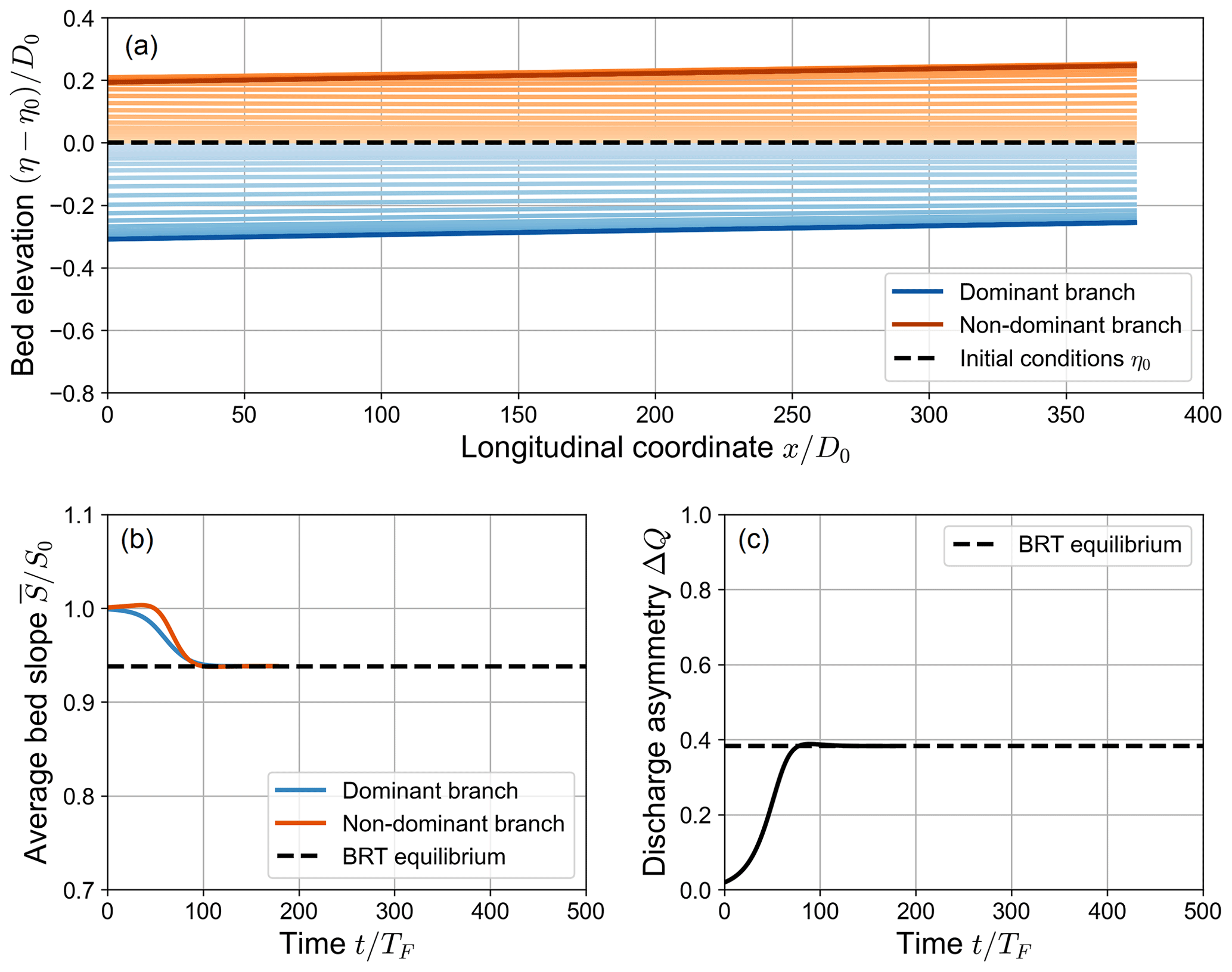
Figure 3Spatial (a) and temporal (b, c) evolution of a fully active numerical simulation, where the long-term state matches the equilibrium solution of the BRT model (β0=15, θ0=0.07, C=12, transport formula of Meyer-Peter and Müller, 1948). The upper panel shows the variation over time of the bed elevation profiles with respect to the initial bed profile η0 (dashed line). Note that both the longitudinal coordinate x and the bed elevation variation η−η0 are scaled with the reference water depth D0. The profiles are sampled with a constant time step of , where TF is defined as in Eq. (16). Panel (b) shows the evolution of the average bed slope of the branches, scaled with the initial bed slope S0. Panel (c) shows the evolution over time of the water discharge asymmetry ΔQ, defined as in Eq. (14). In (b) and (c), the dashed line indicates the equilibrium solution foreseen by the BRT model.
In the first stage, the bed elevation gap between the branches – i.e. the “inlet step” defined by BRT – grows over time following an exponential trend. Specifically, while the branch carrying an increasingly larger fraction of the incoming water discharge (the “dominant” branch) undergoes an erosion process, the other branch (the “non-dominant” branch) undergoes a deposition process. As these two opposite processes develop, the bed slopes of the branches do not vary significantly with respect to their initial value S0. On the contrary, the water discharge asymmetry ΔQ grows exponentially over time (see Fig. 3). The amplification of the degree of asymmetry of the bifurcation in this stage closely matches that resulting from a linear stability analysis of the system of equations of the BRT model, as recently shown by Ragno (2023).
In the second stage of these simulations, nonlinear effects become dominant as the overall bed elevation and the bed slopes of the branches further evolve. The bed slopes of both branches decrease over time, approaching the equilibrium value foreseen by the BRT model, while the discharge asymmetry ΔQ keeps growing until it reaches a maximum value (see Fig. 3). In the third stage, after the maximum of ΔQ is reached, the water discharge asymmetry of the bifurcation decreases, showing an upward-concave trend over time, until it reaches its equilibrium value.
It is worth noticing that there is a non-negligible difference between the maximum value of ΔQ reached at the end of the second stage and its long-term equilibrium value. From now on, we will refer to this difference as “overshoot”, as the simulated value of ΔQ goes beyond the equilibrium value predicted by the analytical BRT model. The overshoot is due to the morphodynamic evolution of the non-dominant branch: the temporary increase in ΔQ is in fact caused by an excess of deposition with respect to the final state that occurs at the inlet of the branch. This temporary increase in the bed elevation of the non-dominant branch causes a decrease in the water discharge entering that branch, thus increasing the water discharge asymmetry ΔQ. This phenomenon may play an important role in determining the long-term state of the bifurcation, as will be discussed later in this section.
As a result of these processes, the bifurcation eventually reaches a long-term state that matches the equilibrium configuration foreseen by the analytical BRT model. In this equilibrium state, both branches are characterized by uniform flow, with constant water depth and bed slope over their length. Since the widths of the branches are both equal to half the width of the upstream channel, the equilibrium value of the bed slopes must always be lower than the initial bed slope S0 to ensure the conservation of sediment mass. Under equilibrium conditions, the inlet step ensures that the transverse sediment flux at the node balances the difference between the transport capacities of the downstream branches, as results from the BRT bulk relationship (Eq. 7).
When β0>βNT, the evolutionary trajectory of the bifurcation does not lead it to reach the equilibrium foreseen by the BRT model as it does for fully active simulations. An example of this type of simulation is represented in Fig. 4. By comparing the evolution over time of the discharge asymmetry ΔQ of this type of simulation (Fig. 4c) with that of fully active simulations (Fig. 3c), one can see that the first two stages qualitatively resemble each other. However, contrary to fully active simulations, at the end of the second stage of simulations where β0>βNT the transport capacity of the non-dominant branch becomes negligible. As a result, the dominant branch is fed with all the incoming sediment discharge, and, most importantly, the non-dominant branch is not able to adjust its bed slope over time anymore. After this “freezing” of the bed slope of the non-dominant branch, the water discharge and the average water depth of the dominant branch considerably increase over time, while its bed slope decreases. This leads to an overall degradation of the branch. Since the non-dominant branch is no longer capable of modifying its morphology, this degradation sharply increases the difference in water depth between the branches, as the water level is prescribed to be the same at the inlets of the branches. The discharge asymmetry ΔQ keeps increasing as well, asymptotically reaching a much larger equilibrium value than that foreseen by the BRT model (see Fig. 4).
At equilibrium, the bed slope of the dominant branch is significantly lower than the equilibrium slope predicted by BRT. On the contrary, the bed slope of the non-dominant branch remains close to the slope S0 prescribed as an initial condition. This is due to the fact that, as in the fully active simulations, the bed slope of both branches does not vary significantly in the early evolutionary stages, while the inlet elevation gap grows over time. The equilibrium configurations of the two bifurcates also differ in terms of water surface profile. While the dominant branch is characterized by uniform flow conditions, the water surface along the non-dominant branch follows an upward-concave profile. The transport capacity being equal to zero along this branch, the backwater curve does not imply an ongoing morphodynamic evolution and is therefore compatible with an equilibrium condition.
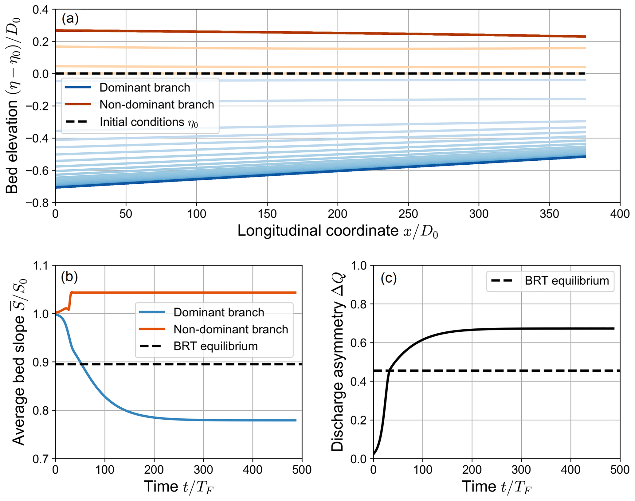
Figure 4Spatial (a) and temporal (b, c) evolution of a numerical simulation where a partial avulsion occurs (β0=20, θ0=0.07, C=12, transport formula of Meyer-Peter and Müller, 1948). The upper panel shows the variation over time of the bed elevation profiles with respect to the initial bed profile η0 (dashed line). Note that both the longitudinal coordinate x and the bed elevation variation η−η0 are scaled with the reference water depth D0. The profiles are sampled with a constant dimensionless time step of , where TF is defined as in Eq. (16). Panel (a) shows the evolution of the average bed slope of the branches, scaled with the initial bed slope S0. Panel (b) shows the evolution over time of the water discharge asymmetry ΔQ, defined as in Eq. (14). In (b) and (c), the dashed line indicates the equilibrium solution foreseen by the BRT model.
It is worth noticing that the two types of equilibrium configurations described above show a remarkably different dependency on the governing parameters. As shown in Fig. 5, the equilibrium configuration of a fully active bifurcation (i.e. when ) does not depend on the length of the bifurcates, as foreseen by the BRT model, the resulting asymmetry being mainly governed by the parameters of the reference upstream flow (i.e. the aspect ratio β0). On the contrary, when a partial avulsion occurs the final configuration also exhibits a sharp dependence on the length of the downstream branches. Specifically, bifurcations with longer branches show a larger discharge asymmetry, a lower bed slope of the dominant branch, and – as a result – a larger overall degradation of the dominant branch itself, as shown by the considerably lower values of . The scenario depicted in Fig. 5 does not qualitatively change when changing the reference Shields stress θ0 but for the values of the critical and the no-transport aspect ratio, whose dependence on θ0 is illustrated in Fig. 1.
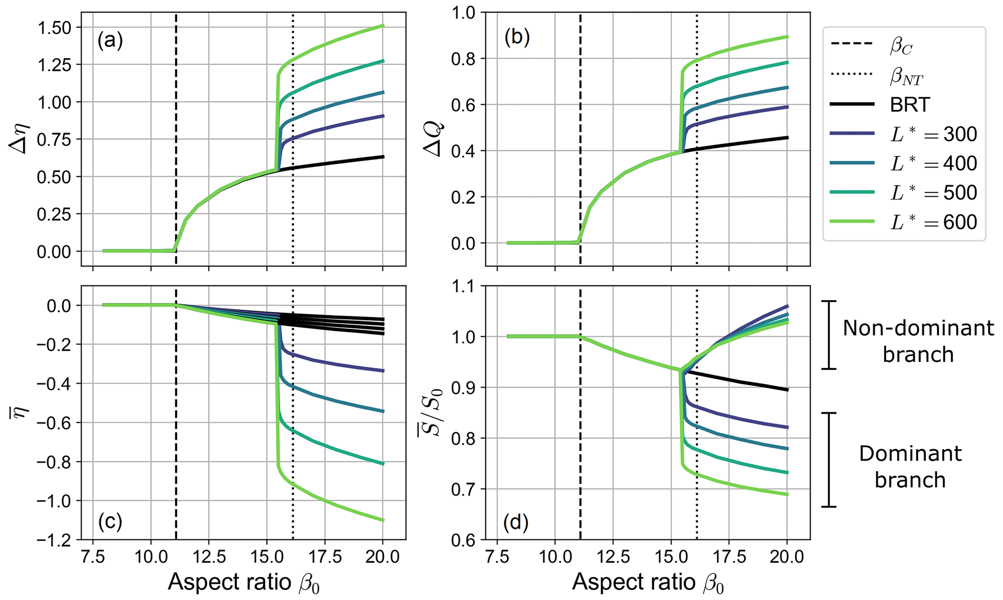
Figure 5Long-term equilibrium states of a free bifurcation: the four panels show the dependence on the aspect ratio β0 of the inlet step Δη, the water discharge asymmetry ΔQ, the average bed elevation at the inlets of the branches , and the bed slope averaged over the branch for different values of the nondimensional length of the bifurcates (, transport formula of Meyer-Peter and Müller, 1948). Solid black lines indicate the equilibrium solutions computed by means of the BRT model. Dashed and dotted lines represent the critical aspect ratio βC and the no-transport aspect ratio βNT, respectively.
The results of numerical simulations therefore suggest that in the case of a partial avulsion the equilibrium state gets more unbalanced as the dimensionless length of the bifurcates increases. Interestingly, by further increasing the length of the branches the evolution of the bifurcation eventually leads to the complete abandonment of the non-dominant branch. In these cases, which we call “full avulsions”, the dominant branch carries all the incoming water and sediment discharges.
Figure 5 also shows that the exact value of β0 above which partial avulsions occur in the numerical simulations is slightly lower than the threshold value βNT computed analytically by means of the BRT model (see dotted lines in the figure). This offset is due to the overshoot phenomenon: if the temporary decrease in the water discharge flowing in the non-dominant branch is large enough, the transport capacity of the branch may drop to zero, thus causing a partial avulsion. Overall, the dependence of the amplitude of the overshoot on the length of the bifurcates is rather weak, as shown by Fig. 6a. Thus, the threshold for β0 for which a partial avulsion occurs in the numerical simulations is almost independent of the length of downstream branches.
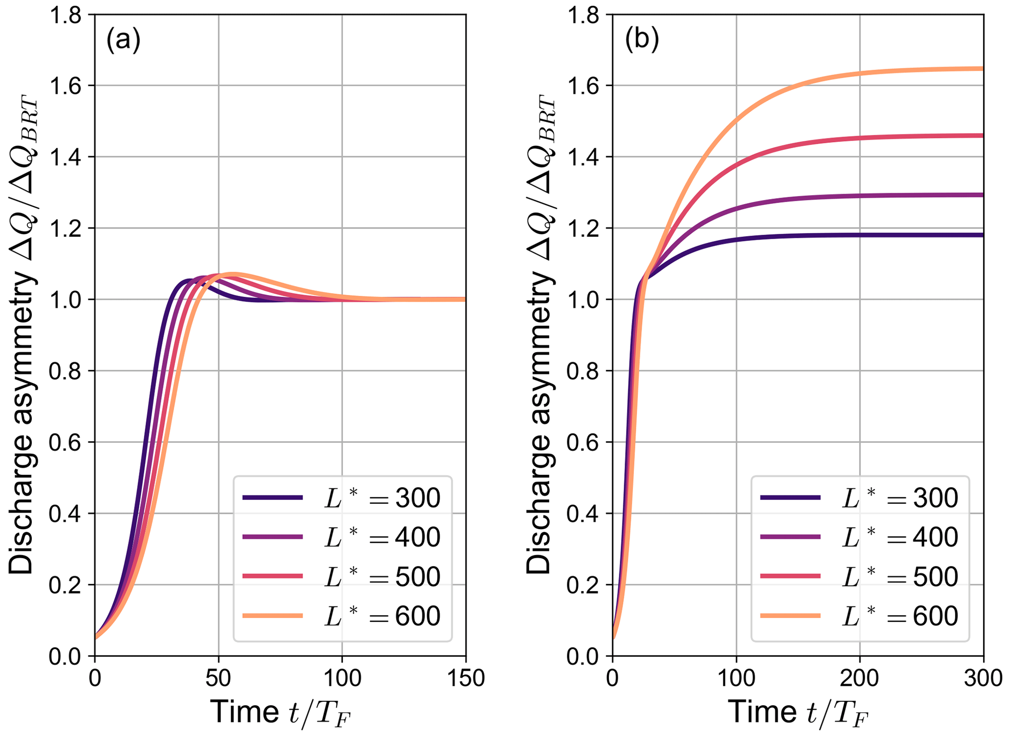
Figure 6The variation over time of the ratio between the simulated discharge asymmetry ΔQ and the equilibrium value foreseen by the BRT model ΔQBRT for different values of the dimensionless length of the bifurcates : (a) and (b) (θ0=0.07, C=12, transport formula of Parker, 1978). The time t is made dimensionless by means of the Exner timescale TF, defined as in Eq. (16).
Figure 6b illustrates how the system evolves in time towards conditions of partial avulsion when β0>βNT. After the initial phase, in which the discharge asymmetry weakly depends on the length L*, an abrupt change is observed as ΔQ exceeds ΔQBRT, when one of the bifurcates becomes no longer able to transport sediments. After this point, the evolution significantly depends on L*, with longer branches leading to a larger discharge asymmetry and requiring a longer time to reach the final equilibrium configuration.
Based on the results of numerical simulations, we can therefore identify different categories of the long-term equilibrium state of a free bifurcation in the plane, as reported in Fig. 7. When β0 is lower than the critical aspect ratio βC, all stable equilibrium states of the bifurcation are balanced, i.e. show an even partitioning of water and solid discharge. Instead, when β0>βC the bifurcation evolves towards a stable and unbalanced equilibrium state, where both branches effectively carry sediments (fully active simulations). When β0 exceeds a second threshold βNT, which is numerically found to be slightly lower than the no-transport threshold predicted analytically, a partial avulsion occurs during the evolution of the bifurcation. In this case, the equilibrium state can be of two types, depending on the value of the dimensionless length of the bifurcates L*. For lower values of L*, the non-transporting branch remains open, although the water discharge asymmetry is much larger than that resulting in the fully active region and also depends on the length of the branches, while it keeps a similar dependency on β0. At larger L* values, a full avulsion occurs and the non-dominant branch is completely abandoned. As suggested by Fig. 7, the threshold value of L* for which a full avulsion occurs is weakly dependent on the upstream aspect ratio β0.
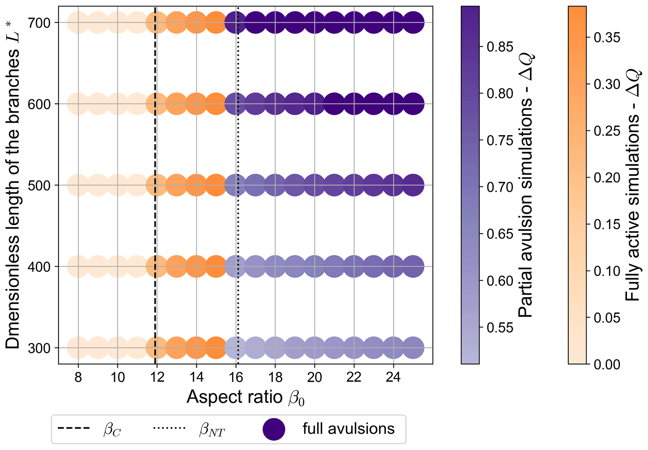
Figure 7Equilibrium configurations of a free bifurcation for different values of the dimensionless length of the downstream branches L* and of the aspect ratio β0 (θ0=0.07, C=12, transport formula of Meyer-Peter and Müller, 1948). Each point corresponds to a single numerical simulation. Reddish colours indicate fully active states, where the discharge asymmetry ΔQ predicted by BRT is attained. Bluish tones indicate partial avulsion states, in which one of the bifurcates does not transport sediments, while dark blue dots indicate states where one of the branches is completely abandoned (ΔQ≃1, full avulsions). Note that the value of the reference Shields stress is the same for all simulations.
The results of numerical simulations reported in the previous section suggest that under conditions of partial avulsion the long-term equilibrium state of a freely evolving bifurcation significantly differs from that predicted by the analytical BRT model. Nonetheless, in this section we show how the equilibrium value of the discharge asymmetry can still be predicted by a simple analytical model by introducing appropriate hypotheses that are supported by information retrieved from numerical simulations.
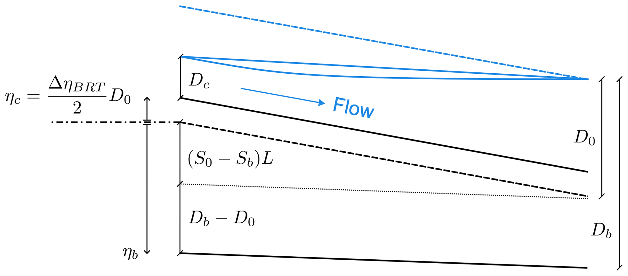
Figure 8Schematic view of two anabranches that undergo a partial avulsion. The bed elevation and water surface profiles are shown for both the initial condition (dashed lines) and long-term configuration (solid lines). η stands for the bed elevation at the inlet of the bifurcates, while S is the longitudinal bed slope, L is the length of both branches, and D is the water depth. The subscripts b and c refer to the dominant and non-dominant branch, respectively, while the subscript 0 denotes the initial reference conditions, which correspond to the initial conditions of the downstream branches. The dash-dotted line indicates the reference level for the bed elevation η, while the dotted line is plotted to highlight the two contributions to the bed elevation ηb appearing in Eq. (22).
We consider the long-term state of an initially balanced bifurcation depicted in Fig. 8, where the shoaling branch c is not able to effectively transport sediments. As in the BRT model, the upstream water (Q0) and sediment (Qs0) supplies are given, while the water level at the downstream end of the branches hd is fixed and defined by the reference water depth D0. However, in this case two additional pieces of information are required to close the mathematical formulation of the equilibrium state, namely the slope Sc and the inlet bed elevation ηc of the shoaling branch. In fact, their actual value results from the evolutionary process of the bifurcation, being determined when the transport capacity vanishes. Moreover, the sediment transport partition at the node takes a simple form, as all the incoming solid discharge is conveyed by the dominant branch.
Under fully active conditions, both downstream branches evolve towards a uniform flow and sediment transport configuration, in which the water surface and bed elevation profiles are straight and parallel to each other. This implies that the equilibrium bed slopes are the same (Sb=Sc), as assumed by BRT. However, this is no longer the case under partial avulsion conditions because when the transport capacity of the shoaling branch vanishes its bed slope Sc remains constant over time, while the slope Sb of the dominant branch continues to evolve until equilibrium is attained. By looking closely at the transient behaviour of the shoaling branch displayed by numerical simulations, we may observe that the overall homogeneous deposition occurring along the branch causes it to stop transporting sediments before its bed slope changes appreciably. Therefore, numerical results suggest that the slope of the shoaling branch does not vary significantly with respect to the initial condition, so it is reasonable to assume that, at equilibrium
As can be seen in panel (d) of Fig. 5, the error we make by using Eq. (17) is relatively small, namely of order 10−2S0.
Another key difference of partial avulsions with respect to the fully active configurations is the computation of the transverse flux of sediments at the node Qsy. Under fully active conditions Qsy is computed by means of the BRT bulk relationship (Eq. 7) and depends on both the discharge asymmetry and the bed elevation gap between the branches. Under conditions of partial avulsion, the equilibrium value of the transverse flux of sediment at the node is always equal to half the incoming sediment discharge, thus granting solid mass continuity in the node cells, regardless of the bed elevation gap between the branches. Thus, the transverse bed slope adjusts in order to satisfy the relationship between the discharge asymmetry and Qsy defined by Eq. (7). On the other hand, the bed elevation gap between the downstream branches – i.e. the inlet step Δη, as defined in Eq. (14) – is entirely governed by the degradation of the dominant branch that leads it to reach its equilibrium bed slope. Thus, the node cells and the inlet step evolve according to two different mechanisms and do not coincide anymore as they do in fully active conditions. As a result, the system gains a degree of freedom.
To replace the missing condition, we assume that, when the transport capacity of the non-dominant branch vanishes, the inlet step Δη equals the inlet step ΔηBRT foreseen by the BRT model. This assumption is consistent with the numerical results, since the first stages of partial avulsion and fully active simulations evolve in a very similar manner. This allows us to compute the bed elevation ηc at the inlet of the shoaling channel c, defined with respect to the initial bed elevation, as
We also note that the variations of discharge asymmetry after the freezing of the shoaling branch imply that flow conditions do not keep uniform throughout the channel. Specifically, the reduction of the water discharge Qc and the fixed water surface elevation at the downstream end of both branches produce an upward-concave water surface profile in the shoaling branch, as illustrated in Fig. 8. Nonetheless, when the branches are longer than the backwater length, it is still possible to assume that in the upstream part of the shoaling branch the flow keeps nearly uniform. This allows us to consider the following uniform flow relations for both branches:
where the water fluxes Qb and Qc can be expressed as functions of the discharge asymmetry ΔQ by considering the water mass conservation:
By substituting Eq. (18) into the nodal condition that sets the same water surface elevation at the inlets of branches b and c, we obtain
where the bed elevation at the inlet of the dominant branch ηb is given by the following geometrical relation, illustrated by Fig. 8:
The system of equations is finally completed by the sediment mass conservation, which under partial avulsion conditions becomes particularly simple, as the entire sediment supply is carried by the dominant branch b:
where the Shields stress θb takes the form
Summarizing, the analytical model for the long-term state of bifurcations under partial avulsion conditions can be cast into a system of four algebraic equations in terms of the four unknowns Sb, Db, Dc, and ΔQ. Specifically, by substituting Eq. (19a) into Eq. (20), substituting Eq. (22) into Eq. (21), and using Eqs. (23) and (24) we obtain
Despite its approximate nature, our simple analytical model proves capable of capturing the key ingredients that determine the equilibrium configurations reached by numerical simulations in which a partial avulsion occurs. As shown by Fig. 9, the equilibrium discharge asymmetry ΔQ foreseen by the analytical model closely matches that obtained in numerical simulations, with an average relative accuracy of less than 3 %. Specifically, our simplified model is able to correctly reproduce the dependence of ΔQ on both the aspect ratio β0 and the dimensionless channel length L*. On the contrary, the equilibrium values of ΔQ computed using the BRT model, besides being independent of the length of the bifurcates, are considerably lower than those shown by numerical simulations, although the dependence of ΔQ on the aspect ratio β0 is similar.
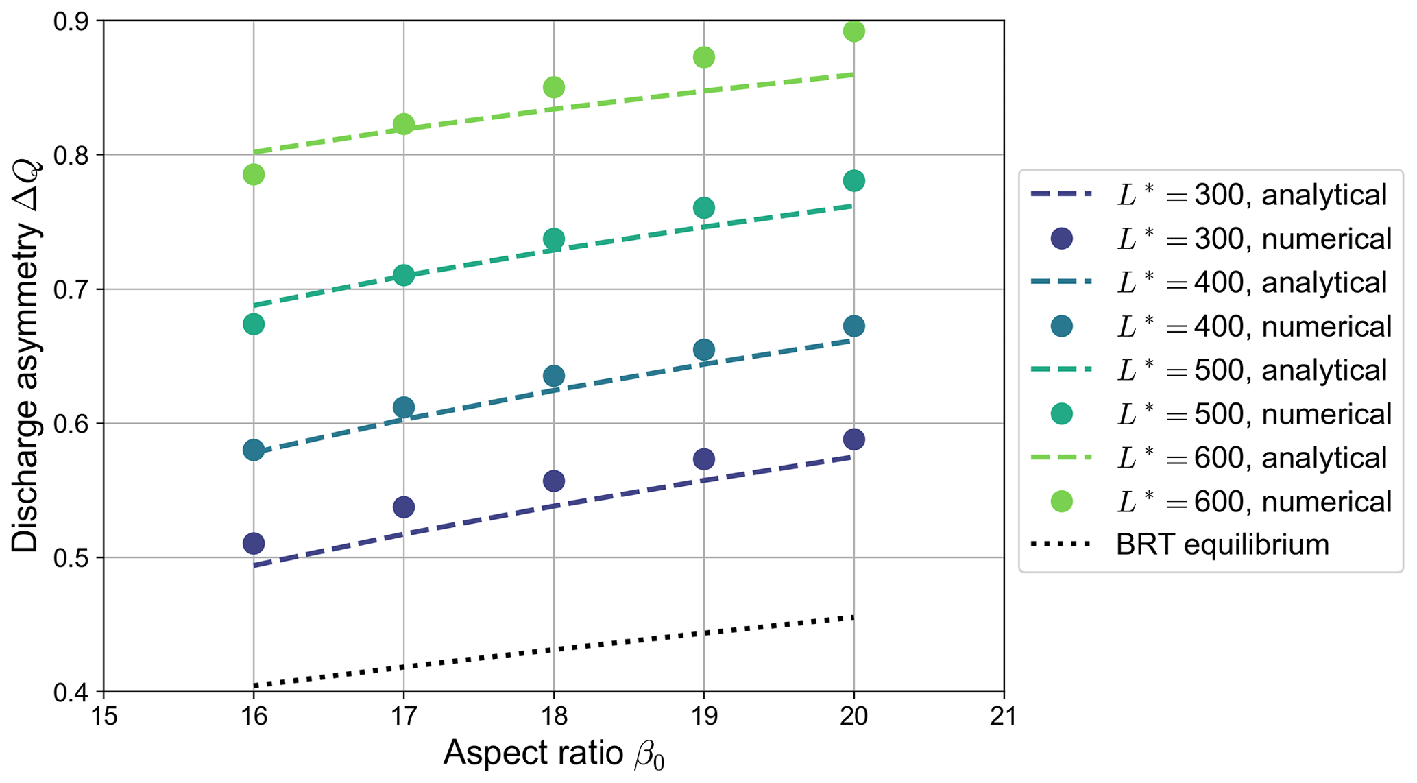
Figure 9Comparison between the equilibrium values of the discharge asymmetry ΔQ of bifurcations undergoing partial avulsion as computed by numerical simulations (dots) and those predicted by the analytical model (dashed lines) for different values of the dimensionless length of the bifurcates (, transport formula of Meyer-Peter and Müller, 1948). Each dot represents the outcome of a single numerical simulation. The dotted line indicates the equilibrium solution computed by means of the BRT model, which is independent of the length of the branches.
The analytical model also makes it possible to determine the marginal conditions for which one of the bifurcates closes completely (full avulsion) and to compute the associated avulsion length LAV. This is accomplished by setting Dc=0 in Eq. (25a) and isolating the length as
The resulting expression highlights the key ingredients that determine the avulsion length, as all terms on the right-hand side of Eq. (26) bring a precise physical meaning. Specifically, the first factor is the backwater length:
which provides the length scale of LAV. Furthermore, the numerator of the second factor accounts for the aggradation experienced by the non-dominant branch until it stops transporting sediment, while the denominator holds the contribution of the incision of the dominant branch. The latter term can be determined from Eq. (25b) by setting ΔQ=1 and using Eq. (24) in the form
This allows us to rewrite Eq. (26) as
where θb can be calculated from mass conservation (Eq. 23).
Results reported in Fig. 10a reveal that, for typical parameter values of gravel-bed rivers, the avulsion length is of the order of several hundred times the upstream flow depth. Furthermore, its dimensionless value exhibits a decreasing trend with both the Shields stress θ0 and the aspect ratio β0. The former inverse dependence is mainly driven by the role of the channel slope S0, while the latter is due to the increase in the term ΔηBRT with β0. Interestingly, when we filter out the main effect of S0 by scaling the avulsion length LAV with the backwater length LB, the dependence of the avulsion length on the Shields stress is reversed, as shown by Fig. 10b.
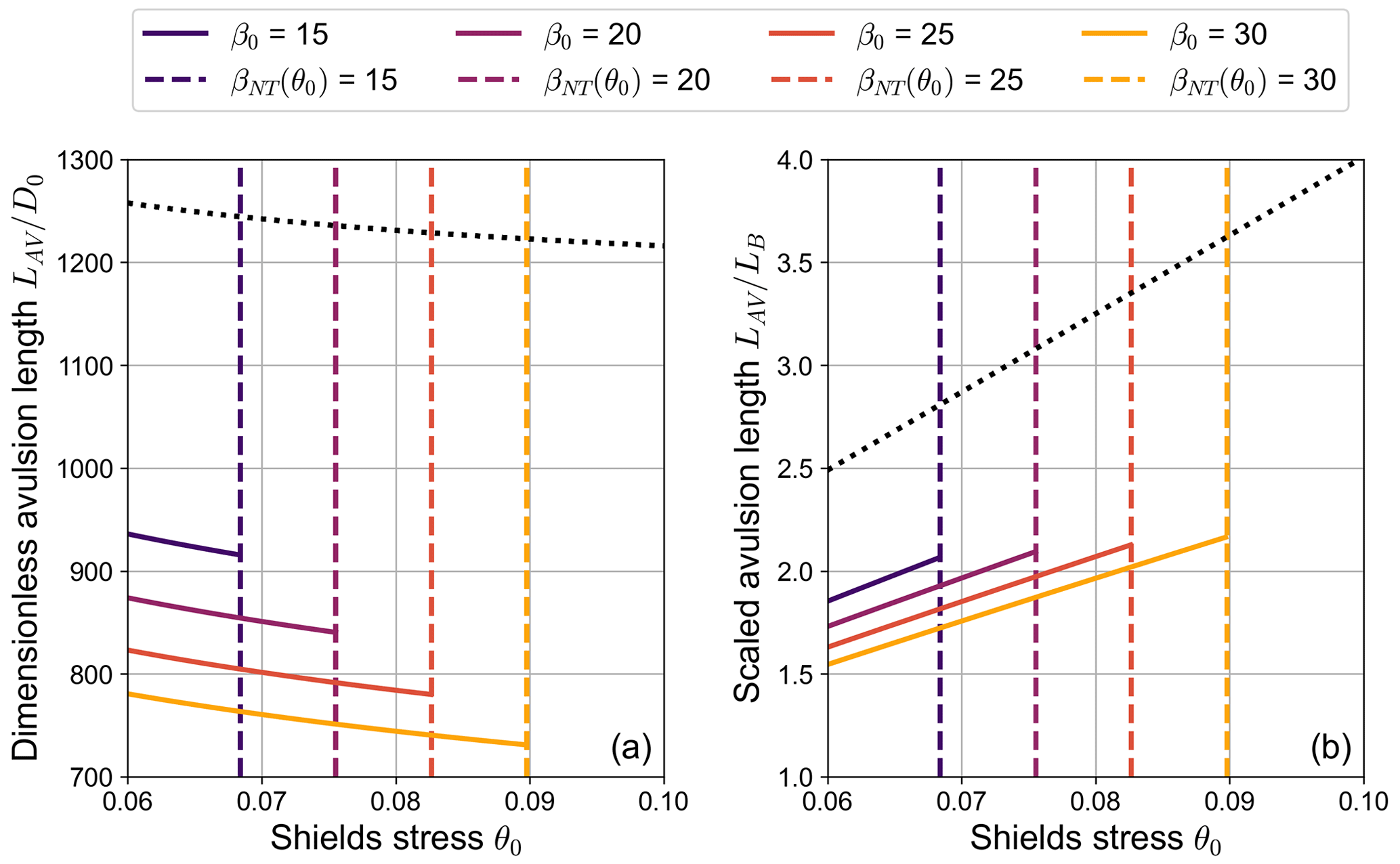
Figure 10Dependence of (a) the dimensionless avulsion length and (b) the scaled avulsion length on the Shields stress θ0 for different values of the aspect ratio β0, as obtained from Eq. (29). Vertical dashed lines indicate the value of the Shields stress for which β0=βNT, thus representing the boundary of the region of validity of the analytical model. The dotted line indicates the upper bound for LAV, obtained by neglecting the β0-dependent term ΔηBRT (C=12, transport formula by Meyer-Peter and Müller, 1948).
The formulation of a new evolutionary model for a free bifurcation allowed us to study the equilibrium states in so-called partial avulsion conditions, in which the flow velocity in one of the bifurcates is not sufficient to effectively transport sediments. In these conditions, the resulting equilibrium configuration turns out to be very different from that predicted by the Bolla Pittaluga et al. (2003) model. Specifically, the resulting long-term equilibrium solution is considerably more asymmetrical, and the inlet step is significantly higher. This happens because the bed slope of the shoaling branch is no longer able to adjust when sediment transport vanishes, while the dominant branch unavoidably undergoes a bed degradation process, which enhances both the inlet step and the discharge asymmetry. Bed degradation increases with the length of the branches, which therefore becomes a key control for the equilibrium configuration.
Consistent with Fig. 1, partial avulsions occur when the aspect ratio of the main channel exceeds the threshold value βNT. However, the actual value of the threshold displayed by simulations turns out to be slightly lower due to an overshoot phenomenon; i.e. in the transitory phase the discharge asymmetry reaches a value that exceeds the long-term equilibrium value. Moreover, the actual threshold for numerical simulations to undergo a partial avulsion may be further reduced with respect to the theoretical value βNT, depending on the behaviour of the transport formula near critical conditions. For example, when considering the transport formula of Parker (1978), the bed evolution of the non-dominant branch “freezes” when the Shields stress is only slightly above the critical threshold θcr=0.03. This occurs because what actually determines the transition from a fully active condition to partial avulsion is the ratio between the evolutionary timescales of the branches. Specifically, if the dominant branch degrades too quickly with respect to the other branch, it starts capturing more discharge than that foreseen by the BRT model, which rapidly leads to partial avulsion conditions. It is worth noting that, for the same reason, partial avulsions also occur when employing a transport formula that does not consider a critical threshold (e.g. Parker, 1990). In this case, the analytical threshold βNT beyond which the BRT model does not work can no longer be defined. However, numerical simulations still show a threshold for β0 above which partial avulsions occur. In these conditions, the shoaling branch practically freezes even though a minimal amount of sediment transport is still present, causing the bifurcation to reach a strongly unbalanced long-term configuration.
The analytical model developed in Sect. 4 enables computing the long-term state of bifurcations under conditions of partial avulsion and identifying the key parameters that control the transition between the different kinds of equilibrium configurations shown by numerical simulations and represented in Fig. 7. When combined with the results of the BRT model, the analytical model allows us to draw a complete picture of the nature of the equilibrium solutions in the parameter space, as illustrated in Fig. 11. Specifically, for a given value of the reference Shields stress θ0, four distinct regions are identified:
-
balanced solutions (i.e. ), occurring when the aspect ratio β0 is lower than the length-independent critical threshold βC;
-
unbalanced fully active solutions, where at equilibrium both branches actively transport sediment, occurring when β0 lies between βC and the no-transport threshold βNT;
-
partial avulsion solutions, in which all sediments go in one branch, while a nonzero water discharge flows in the other, occurring when β0>βNT and the length of the branches is shorter than the threshold LAV;
-
full avulsions solutions, where one branch is abandoned and all the incoming water and sediment supplies are carried by the other branch, occurring when the aspect ratio is relatively large and the downstream branches are relatively long (i.e. β0>βNT and L>LAV).
The threshold values βC and βNT increase as the Shields stress increases, and so does the scaled avulsion length , as discussed at the end of Sect. 4.
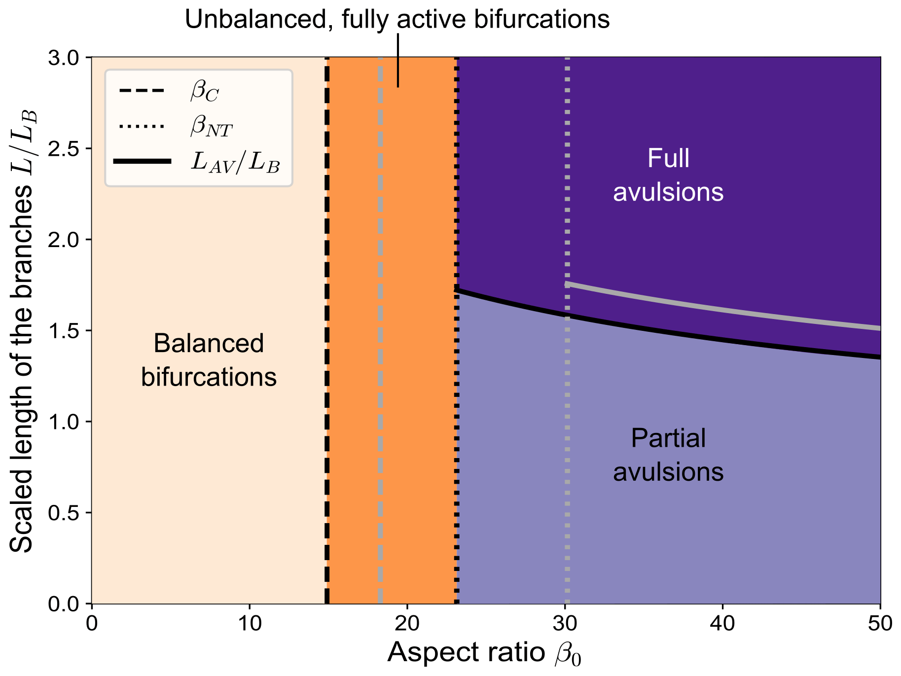
Figure 11The different types of equilibrium configurations of a free bifurcation in the β0 (aspect ratio) − (scaled branch length) parameter space, resulting from the combination of the BRT model and our analytical model (θ0=0.08, transport formula of Meyer-Peter and Müller, 1948). The length of the bifurcates is scaled with the backwater length LB, computed as . The different line styles indicate the critical aspect ratio βC, the aspect ratio of no-transport βNT, and the scaled avulsion length resulting from Eq. (29). The grey lines show how these thresholds change when considering a slightly higher value of the Shields stress (θ0=0.09).
A direct comparison between our model and experimental data is difficult, since available data from physical models are scarce and often focused on the effect of external forcing factors. For example, the laboratory experiments by Salter et al. (2019) were tailored to depositional environments and reproduced bifurcations with prograding branches, while Szewczyk et al. (2020) analysed the influence on the water discharge partition of changing the bifurcation angle for values of the aspect ratio β0 much smaller than the no-transport threshold βNT. To the authors' knowledge, the laboratory experiments by Bertoldi and Tubino (2007) are the only ones that analysed how initially balanced free bifurcations develop unbalanced equilibrium configurations, possibly leading to partial or full avulsion. Considering this dataset, it is worth noting that the three experimental runs that resulted in a full avulsion featured an aspect ratio close to or larger than the no-transport aspect ratio βNT and a length of the branches larger than the avulsion threshold LAV, consistent with our model predictions.
As shown in Fig. 11, when the downstream branches are sufficiently long, the degradation process can eventually lead to the complete abandonment of the shoaling branch so that water and sediment fluxes are entirely conveyed in a single thread (full avulsion). The branch length at which full avulsion occurs (LAV) is found to scale with the backwater length. This result is consistent with existing studies of river deltas that show how the distance of apex avulsions from the coastline scales with the backwater length (Chatanantavet et al., 2012; Jerolmack and Mohrig, 2007). It is worth remarking that previous studies found this scaling by analysing deposition induced by time-dependent flow discharge, while our study highlights the link between the backwater length and the full avulsion threshold by analysing the interplay between the downstream boundary condition and the incision required for the abandonment of the shoaling channel.
Our analysis provides a clear example of how the complete abandonment of one of the two branches can be caused by the incision of the dominant channel driven by an autogenic mechanism. In general, bed incision takes place whenever the bifurcation becomes unbalanced, as the resulting difference of the Shields stress between the two branches makes them overall more efficient in transporting sediments (Paola, 1996; Ferguson, 2003). Therefore, a smaller slope is sufficient to ensure equilibrium with the imposed sediment supply. This effect is further amplified when the water discharge asymmetry sharply increases due to a partial avulsion. This can provide a mechanistic interpretation of the so-called process of incisional avulsion (Mohrig et al., 2000; Slingerland and Smith, 2004), in which channel abandonment is preceded by headward erosion of the avulsed channel.
The tendency to abandon smaller branches can be seen as a general characteristic of rivers systems undergoing significant incision, such as that produced by a lack of sediment supply. Specifically, discharge asymmetry of river bifurcations generally increases when the overall degradation rate is relatively rapid. In this case, the shoaling branch is not able to keep up with the erosion, thus becoming increasingly super-elevated with respect to the dominant channel. This may provide a way to interpret the morphological evolution of braided rivers under conditions of reduced sediment availability, which typically lead to the simplification of the channel network and eventually to the transition to single-thread configurations (e.g. Germanoski and Schumm, 1993; Marti and Bezzola, 2006; Redolfi and Tubino, 2014).
The numerical and analytical results reported in Figs. 5 an 9 highlight the inadequacy of the BRT model to reproduce the strongly unbalanced long-term configuration of free bifurcations when a branch avulsion occurs, as already pointed out by Kleinhans et al. (2008). They also provide new insight into the long-debated question of the role of the nodal condition for sediment partitioning. In fully active conditions, the inlet step between the downstream branches of an unbalanced bifurcation generates a lateral bed slope at the node such that the transverse sediment flux Qsy compensates for the imbalance of transport capacities between the bifurcates themselves. The efficiency of this lateral deflection thus plays a key role in determining the equilibrium configuration of the bifurcation, as shown by the BRT model. On the contrary, under partial (or full) avulsion conditions the incoming sediment supply is entirely steered towards the dominant branch, regardless of the inlet step. After the shoaling branch gets morphodynamically inactive, the development of the inlet step between the bifurcates is entirely governed by the evolution of the dominant branch and specifically by the changes in its bed slope and water depth that are necessary to attain a morphodynamic equilibrium.
Under this condition, the transverse flux of sediments Qsy is mainly driven by flow exchange (the first term on the left-hand side of the nodal relationship in Eq. 7), while the lateral deflection due to transverse slope (the second term on the left-hand side of Eq. 7) plays a minor role in determining the equilibrium bifurcation asymmetry. As a result, the bed elevation gap between the node cells of the BRT model (see Fig. 2) simply yields the residual contribution ensuring the condition at equilibrium, and it no longer aligns with the downstream inlet step. As can be seen in Fig. 4, the resulting evolution of the dominant branch shows no discontinuity between the fully active initial stages and the partial avulsion long-term state. In fact, the transverse flux returned by Eq. (7) produces a smooth transient behaviour in the dominant channel and ensures mass conservation.
In general, the timescale of the adaptation of the bifurcation to its long-term state is much longer than that governing the first evolutionary stages, as shown for example by the lower right panel of Fig. 4. This happens because the dominant branch needs time to adapt its bed slope to the equilibrium value. Meanwhile, other upstream or downstream effects may influence the evolutionary process of the bifurcation, namely the effect of changes in sediment supply, the adaptation of channel width, and variations of the downstream water level (e.g. sea level rise). While our model can be straightforwardly extended to reproduce such effects, further investigation is needed to assess their relevance in determining the bifurcation configuration, depending on the characteristic timescales of the associated processes.
The present formulation is valid under conditions where sediment is dominantly transported as bedload. Although some promising approaches have been proposed (Iwantoro et al., 2021), a systematic understanding of the morphodynamics of channel bifurcations in suspension-dominated channels is still lacking, thus preventing a reliable extension of our model. However, we can expect a similar scenario of transition to the avulsion condition to also occur for sand-bed channels where most sediments are transported in suspension. In this case the higher values of the Shields stress are likely to be associated with a higher threshold βNT so that larger values of the aspect ratio may be needed to reach avulsion conditions.
Finally, it is worth noting that in this work we consider the water discharge to be constant in time. Therefore, the application of the model to unsteady flow conditions is only possible when flow variations are sufficiently slow to be represented as a sequence of quasi-steady states. To account for flow variability it would be possible to define an equivalent, formative value of Q, for example by considering the method of effective discharge proposed by Wolman and Miller (1960), or to adopt a procedure similar to that recently proposed by Carlin et al. (2021) for alternate bars.
In this study we developed a novel 1D numerical model for predicting the evolution of a river bifurcation. Based on numerical findings, we then built a new analytical model, specifically designed to reproduce the equilibrium configuration of a bifurcation under partial avulsion conditions. Coupling the latter model with that proposed by Bolla Pittaluga et al. (2003) provides a suite of analytical tools that covers the full range of possible long-term states of a free bifurcation in the controlling parameter space, namely the aspect ratio and the Shields stress.
The combined analysis of the numerical and analytical model yields the following conclusions.
-
When the aspect ratio of the main channel exceeds the threshold value βNT, the bifurcation undergoes partial avulsion conditions, in which the shoaling channel is no longer able to effectively transport sediments.
-
Under partial avulsion conditions, the dominant channel is subject to degradation, while the morphological evolution of the other branch is inhibited. This produces a significant increase in the inlet step at the entrance of the bifurcates, further enhancing the water discharge entering the dominant channel. This autogenic positive feedback mechanism results in a highly unbalanced equilibrium configuration, whose long-term degree of asymmetry is influenced by the length of the downstream branches.
-
When the dimensionless length of the bifurcates exceeds a threshold value LAV, the discharge asymmetry tends to unity, which implies the complete abandonment of the shoaling channel (full avulsion). Such a threshold length is found to scale with the backwater length.
Overall, this work allows us to draw a complete picture of conditions that may lead to the abandonment of one branch in “free” river bifurcations for the first time. This provides the basis for more detailed studies about the role of other factors – such as flow variability, sea level rise, and bank erosion – in determining the long-term evolution of bifurcations. Furthermore, our study gives valuable insights for the design of sustainable river restoration interventions aimed at promoting the formation of rich, multi-thread channel patterns.
The code used for the numerical model is freely available at https://doi.org/10.5281/zenodo.10079752 (Barile, 2023).
The dataset of the laboratory experiments by Bertoldi and Tubino (2007) is available in the Supplement of their article.
GB, MR, and MT conceptualized the work and designed the methodology. GB developed the software and wrote the paper draft, which was reviewed and edited by all authors.
The contact author has declared that none of the authors has any competing interests.
Publisher's note: Copernicus Publications remains neutral with regard to jurisdictional claims made in the text, published maps, institutional affiliations, or any other geographical representation in this paper. While Copernicus Publications makes every effort to include appropriate place names, the final responsibility lies with the authors.
We thank both reviewers for their inspiring comments and suggestions, which helped to improve the article.
This work has been supported by the Italian Ministry of Universities and Research (MUR) in the framework of the project DICAM-EXC (Departments of Excellence 2023–2027, grant L232/2016), the consortium iNEST (Interconnected Nord-Est Innovation Ecosystem) funded by the European Union Next-GenerationEU (Piano Nazionale di Ripresa e Resilienza PNRR – Missione 4 Componente 2, Investimento 1.5 – D.D. 1058 23/06/2022, ECS_00000043), and the “Agenzia Provinciale per le Risorse Idriche e l’Energia” (APRIE) of the Province of Trento (Italy).
This paper was edited by Kieran Dunne and reviewed by V. Voller and Lorenzo Durante.
Baar, A. W., de Smit, J., Uijttewaal, W. S. J., and Kleinhans, M. G.: Sediment Transport of Fine Sand to Fine Gravel on Transverse Bed Slopes in Rotating Annular Flume Experiments, Water Resour. Res., 54, 19–45, https://doi.org/10.1002/2017WR020604, 2018. a
Barile, G.: A Python 1D numerical model of a river bifurcation, Zenodo [code], https://doi.org/10.5281/zenodo.10079752, 2023. a
Bertoldi, W. and Tubino, M.: River bifurcations: Experimental observations on equilibrium configurations, Water Resour. Res., 43, 1–10, https://doi.org/10.1029/2007WR005907, 2007. a, b
Bertoldi, W., Zanoni, L., Miori, S., Repetto, R., and Tubino, M.: Interaction between migrating bars and bifurcations in gravel bed rivers, Water Resources Research, 45, 1–12, https://doi.org/10.1029/2008WR007086, 2009. a
Bolla Pittaluga, M., Repetto, R., and Tubino, M.: Channel bifurcation in braided rivers: Equilibrium configurations and stability, Water Resour. Res., 39, 1–13, https://doi.org/10.1029/2001WR001112, 2003. a, b, c, d, e, f
Carlin, M., Redolfi, M., and Tubino, M.: The Long-Term Response of Alternate Bars to the Hydrological Regime, Water Resour. Res., 57, e2020WR029314, https://doi.org/10.1029/2020WR029314, 2021. a
Chatanantavet, P., Lamb, M. P., and Nittrouer, J. A.: Backwater Controls of Avulsion Location on Deltas, Geophys. Res. Lett., 39, L01402, https://doi.org/10.1029/2011GL050197, 2012. a
Edmonds, D. A. and Slingerland, R. L.: Stability of delta distributary networks and their bifurcations, Water Resour. Res., 44, 9426, https://doi.org/10.1029/2008WR006992, 2008. a
Edmonds, D. A., Paola, C., Hoyal, D. C. J. D., and Sheets, B. A.: Quantitative Metrics That Describe River Deltas and Their Channel Networks, J. Geophys. Res., 116, F04022, https://doi.org/10.1029/2010JF001955, 2011. a
Ferguson, R. I.: Understanding Braiding Processes in Gravel-Bed Rivers: Progress and Unsolved Problems, Geological Society, London, Special Publications, 75, 73–87, https://doi.org/10.1144/GSL.SP.1993.075.01.03, 1993. a
Ferguson, R. I.: The missing dimension: Effects of lateral variation on 1-D calculations of fluvial bedload transport, Geomorphology, 56, 1–14, https://doi.org/10.1016/S0169-555X(03)00042-4, 2003. a
Field, J.: Channel Avulsion on Alluvial Fans in Southern Arizona, Geomorphology, 37, 93–104, https://doi.org/10.1016/S0169-555X(00)00064-7, 2001. a
Germanoski, D. and Schumm, S. A.: Changes in Braided River Morphology Resulting from Aggradation and Degradation, J. Geol., 101, 451–466, https://doi.org/10.1086/648239, 1993. a
Habersack, H. and Piégay, H.: 27 River restoration in the Alps and their surroundings: past experience and future challenges, Developments in Earth Surface Processes, 11, 703–735, https://doi.org/10.1016/S0928-2025(07)11161-5, 2007. a
Iwantoro, A. P., Vegt, M., and Kleinhans, M. G.: Effects of sediment grain size and channel slope on the stability of river bifurcations, Earth Surf. Proc. Land., 46, 2004–2018, https://doi.org/10.1002/esp.5141, 2021. a
Iwantoro, A. P., van der Vegt, M., and Kleinhans, M. G.: Stability and Asymmetry of Tide-Influenced River Bifurcations, J. Geophys. Res.-Earth, 127, e2021JF006282, https://doi.org/10.1029/2021JF006282, 2022. a, b
Jerolmack, D. J. and Mohrig, D.: Conditions for branching in depositional rives, Geology, 35, 463–466, https://doi.org/10.1130/G23308A.1, 2007. a
Kleinhans, M. G., Jagers, H. R., Mosselman, E., and Sloff, C. J.: Bifurcation dynamics and avulsion duration in meandering rivers by one-dimensional and three-dimensional models, Water Resour. Res., 44, W08454, https://doi.org/10.1029/2007WR005912, 2008. a, b, c, d
Kleinhans, M. G., de Haas, T., Lavooi, E., and Makaske, B.: Evaluating competing hypotheses for the origin and dynamics of river anastomosis, Earth Surf. Proc. Land., 37, 1337–1351, https://doi.org/10.1002/esp.3282, 2012. a
Le, T. B., Crosato, A., Mosselman, E., and Uijttewaal, W. S.: On the stability of river bifurcations created by longitudinal training walls. Numerical investigation, Adv. Water Resour., 113, 112–125, https://doi.org/10.1016/j.advwatres.2018.01.012, 2018. a
Leddy, J. O., Ashworth, P. J., and Best, J. L.: Mechanisms of Anabranch Avulsion within Gravel-Bed Braided Rivers: Observations from a Scaled Physical Model, Geological Society, London, Special Publications, 75, 119–127, https://doi.org/10.1144/GSL.SP.1993.075.01.07, 1993. a
Marti, C. and Bezzola, G. R.: Bed load transport in braided gravel-bed rivers, Braided Rivers: Process, Deposits, Ecology and Management. Special Publication, 36, 199–215, 2006. a
Mendoza, A., Berezowsky, M., Caballero, C., and Arganis-Juárez, M.: Alteration of the flow distribution at a river bifurcation caused by a system of upstream dams: Case of the Grijalva River basin, Mexico, Earth Surf. Proc. Land., 47, 509–521, https://doi.org/10.1002/esp.5265, 2022. a
Meyer-Peter, E. and Müller, R.: Formulas for Bed-Load Transport, in: IAHSR 2nd Meeting, Stockholm, Appendix 2, IAHR, http://resolver.tudelft.nl/uuid:4fda9b61-be28-4703-ab06-43cdc2a21bd7 (last access: 22 December 2023), 1948. a, b, c, d, e, f, g, h
Mohrig, D., Heller, P. L., Paola, C., and Lyons, W. J.: Interpreting avulsion process from ancient alluvial sequences: Guadalope-Matarranya system (Northern Spain) and Wasatch formation (Western Colorado), Bull. Geol. Soc. Am., 112, 1787–1803, https://doi.org/10.1130/0016-7606(2000)112<1787:IAPFAA>2.0.CO;2, 2000. a
Paola, C.: Incoherent structure: turbulence as a metaphor for stream braiding, Coherent Flow Structures in Open Channels, 65, 705–723, 1996. a
Parker, G.: Self-formed straight rivers with equilibrium banks and mobile bed. Part 2. The gravel river, J. Fluid Mech., 89, 127–146, https://doi.org/10.1017/S0022112078002505, 1978. a, b, c
Parker, G.: Surface-based bedload transport relation for gravel rivers, J. Hydraul. Res., 28, 417–436, https://doi.org/10.1080/00221689009499058, 1990. a
Ragno, N.: Viewing Second-Order Phase Transitions as a Metaphor for River Bifurcations, J. Fluid Mech., 974, A53, https://doi.org/10.1017/jfm.2023.831, 2023. a
Ragno, N., Tambroni, N., and Bolla Pittaluga, M.: Effect of Small Tidal Fluctuations on the Stability and Equilibrium Configurations of Bifurcations, J. Geophys. Res.-Earth, 125, e2020JF005584, https://doi.org/10.1029/2020JF005584, 2020. a
Redolfi, M.: Defining the Length Parameter in River Bifurcation Models: A Theoretical Approach, Earth Surf. Proc. Land., 48, 2121–2132, https://doi.org/10.1002/esp.5673, 2023. a
Redolfi, M. and Tubino, M.: A diffusive 1D model for the evolution of a braided network subject to varying sediment supply, 1153–1161, https://doi.org/10.1201/b17133-155, ISBN 9781138026742, 2014. a
Redolfi, M., Zolezzi, G., and Tubino, M.: Free instability of channel bifurcations and morphodynamic influence, J. Fluid Mech., 799, 476–504, https://doi.org/10.1017/jfm.2016.389, 2016. a
Redolfi, M., Zolezzi, G., and Tubino, M.: Free and forced morphodynamics of river bifurcations, Earth Surf. Proc. Land., 44, 973–987, https://doi.org/10.1002/esp.4561, 2019. a
Salter, G., Paola, C., and Voller, V. R.: Control of Delta Avulsion by Downstream Sediment Sinks, J. Geophys. Res.-Earth, 123, 142–166, https://doi.org/10.1002/2017JF004350, 2018. a, b, c
Salter, G., Voller, V. R., and Paola, C.: How does the downstream boundary affect avulsion dynamics in a laboratory bifurcation?, Earth Surf. Dynam., 7, 911–927, https://doi.org/10.5194/esurf-7-911-2019, 2019. a
Slingerland, R. and Smith, N. D.: River avulsions and their deposits, Annu. Rev. Earth Pl. Sc., 32, 257–285, https://doi.org/10.1146/annurev.earth.32.101802.120201, 2004. a, b
Szewczyk, L., Grimaud, J.-L., and Cojan, I.: Experimental evidence for bifurcation angles control on abandoned channel fill geometry, Earth Surf. Dynam., 8, 275–288, https://doi.org/10.5194/esurf-8-275-2020, 2020. a
Wolman, G. M. and Miller, J. P.: Magnitude and frequency of forces in geomorphic processes, J. Geol., 68, 54–74, https://www.jstor.org/stable/30058255 (last access: 1 January 2024), 1960. a
Zolezzi, G. and Seminara, G.: Downstream and Upstream Influence in River Meandering. Part 1. General Theory and Application to Overdeepening, J. Fluid Mech., 438, 183–211, https://doi.org/10.1017/S002211200100427X, 2001. a