MPeat2D – a fully coupled mechanical–ecohydrological model of peatland development in two dimensions

Higher-dimensional models of peatland development are required to analyse the influence of spatial heterogeneity and complex feedback mechanisms on peatland behaviour. However, the current models exclude the mechanical process that leads to uncertainties in simulating the spatial variability in the water table position, vegetation composition, and peat physical properties. Here, we propose MPeat2D, a peatland development model in two dimensions, which considers mechanical, ecological, and hydrological processes together with the essential feedback from spatial interactions. MPeat2D employs poroelasticity theory that couples fluid flow and solid deformation to model the influence of peat volume changes on peatland ecology and hydrology. To validate the poroelasticity formulation, the comparisons between numerical and analytical solutions of Mandel's problems for two-dimensional test cases are conducted. The application of MPeat2D is illustrated by simulating peatland growth over 5000 years above a flat and impermeable substrate with free-draining boundaries at the edges, using constant and variable climate. In both climatic scenarios, MPeat2D produces lateral variability in the water table depth, which results in the variation in the vegetation composition. Furthermore, the drop in the water table at the margin increases the compaction effect, leading to a higher value of bulk density and a lower value of active porosity and hydraulic conductivity. These spatial variations obtained from MPeat2D are consistent with the field observations, suggesting plausible outputs from the proposed model. By comparing the results of MPeat2D to a one-dimensional model and a two-dimensional model without the mechanical process, we argue that mechanical–ecohydrological feedbacks are important for analysing spatial heterogeneity, shape, carbon accumulation, and resilience of peatlands.

1 Introduction

In this paper, we provide a fully coupled mechanical–ecohydrological model of peatland development in two dimensions (2D). The continuum representation of the peatland employed by the proposed model results in the advancement of peatland modelling, particularly if we consider questions relating to the phenomena for which mechanical process and feedback are essential components. Examples of these phenomena include the analysis of mechanical limits to peatland stability and the relationship between topography, peat physical properties, and carbon accumulation. The purpose of this paper is to explain the formulation of the model, which is developed from an earlier one-dimensional (1D) mechanical–ecohydrological model (Mahdiyasa et al., 2023, 2022). Its application is illustrated through the simulations of the long-term peatland growth over millennia under idealised conditions. To consider the consequences of incorporating spatial variability and mechanical process on the peatland behaviour, we compare our results with the existing peatland growth models, including a 1D model without spatial variability, MPeat (Mahdiyasa et al., 2023, 2022), and a 2D stiff non-continuum model, DigiBog (Baird et al., 2012; Morris et al., 2012).

The spatial variability in the peatland is widely evidenced by the changes in the horizontal and vertical directions of peat physical properties, including bulk density, active porosity, and hydraulic conductivity. The horizontal variation in the hydraulic conductivity was observed by Lapen et al. (2005), who found that hydraulic conductivity is lower at the margin than at the centre based on the field measurements and analysis of a peatland groundwater flow model. Field observations from Baird et al. (2008) and Lewis et al. (2012), who measured lateral variability in the hydraulic conductivity in a raised and a blanket peatland, respectively, agree with the Lapen et al. (2005) finding. Lewis et al. (2012) also observed the lateral variability in bulk density, which increased from the centre toward the margin. In the vertical direction, deeper peat exhibits a higher value of bulk density and a lower value of active porosity and hydraulic conductivity, with abrupt changes occurring between the unsaturated and saturated zones (Clymo, 2004, 1984; Hoag and Price, 1997, 1995; Quinton et al., 2008, 2000; Fraser et al., 2001). Moreover, the meta-analysis from Morris et al. (2022), with an extensive database of hydraulic conductivity and bulk density, also indicates that depth significantly affects these peat physical properties.

As a porous medium with a low value of Young's modulus (Long, 2005; Mesri and Ajlouni, 2007; Boylan et al., 2008; Dykes and Warburton, 2008), the peat body is susceptible to deformation. The deformation is non-uniform throughout the peatland area due to the spatial variations in the water table depth that influence the effective stress (Whittington and Price, 2006; Price, 2003; Price et al., 2005; Waddington et al., 2010). For example, the increase in water table depth at the margin leads to higher bulk density and lower active porosity and hydraulic conductivity, preventing greater water discharge from the deeper peat. Consequently, Lapen et al. (2005) posited that a lower hydraulic conductivity at the margin has a significant influence on maintaining the wet condition at the centre, which in turn affects peat accumulation. Therefore, the spatial variations in the peat physical properties potentially provide essential feedback as the peatland develops.

Higher-dimensional models of peatland development ignore mechanical feedback (e.g. Ingram, 1982; Winston, 1994; Armstrong, 1995; Korhola et al., 1996; Borren and Bleuten, 2006; Baird et al., 2012; Morris et al., 2012; Swinnen et al., 2019) and do not allow the peat volume to change by compaction, which leads to the use of empirical relationships to generate realistic values of bulk density, active porosity, and hydraulic conductivity. For example, Borren and Bleuten (2006) proposed a three-dimensional model (3D) of peatland development based on the groundwater flow model (Boussinesq, 1871) and focused on the ecohydrological feedback between the water table position with peat production and decomposition, following the Clymo (1984) model. The mechanical compaction is assumed to be negligible, and the spatial variations in the bulk density and hydraulic conductivity are obtained based on the empirical relationship between different peatland types consisting of bog, throughflow fen, and fen. DigiBog (Baird et al., 2012; Morris et al., 2012) is a 1D, 2D, or 3D model of peatland development that accommodates the spatial changes in hydraulic conductivity through the differences in remaining mass that are affected by the water table position and decomposition processes (Moore et al., 2005; Quinton et al., 2000). Although DigiBog captures more complex feedback between ecological and hydrological processes than the model from Borren and Bleuten (2006), the omission of mechanical feedback leads to the assumption of constant active porosity and bulk density as the peatland grows. Cobb et al. (2017) developed a 2D tropical peatland growth model to analyse the influence of climate, particularly the rainfall pattern, on carbon storage. This model simulates the dynamics of the water table and peat accumulation through the groundwater flow model (Boussinesq, 1871) and the difference between peat production and decomposition. The carbon storage is estimated from the stable peat surface Laplacian that is affected by the rate of peat production and decomposition. The peat surface Laplacian indicates the curvature of the peat surface, which is calculated as the sum of second derivatives of surface elevation. Although the surface Laplacian provides information related to the peatland morphology, this model ignores the mechanical feedback and assumes a constant value of hydraulic conductivity that becomes the source of uncertainty in estimating the peatland carbon storage.

This paper, therefore, sets out to (1) provide the formulation of a fully coupled mechanical–ecohydrological model of peatland development in 2D called MPeat2D, (2) investigate model outputs in the idealised peatland growth scenario, and (3) analyse the potential consequences of mechanical–ecohydrological feedback on the long-term peatland carbon accumulation and resilience by comparison with other peatland development models. The structure of this paper is presented in three main parts. First, we consider the mathematical formulation, consisting of mechanical, ecological, and hydrological submodels, together with the numerical verification of the MPeat2D. Second, we explain how to implement MPeat2D to simulate long-term peatland growth over millennia and provide examples of model outputs. Third, we examine the implications obtained from MPeat2D to understand peatland behaviour and conclude the analysis by addressing the areas in which further development from the model is required. Although MPeat2D is focused on ombrotrophic peatlands with temperate climates, the framework proposed in this paper could be employed to model the other peatland types.

2 Model formulation and verification

MPeat2D is a fully coupled mechanical, ecological, and hydrological model of long-term peatland growth in two dimensions which takes spatial variability and structure into consideration. MPeat2D is developed based on the continuum concept (Irgens, 2008; Jog, 2015) that assumes peatland constituents, both solid and fluid particles, entirely fill the peatland body. Through this approach, the conservation of mass can be appropriately defined to formulate mechanical processes on the peatland obtained from the coupling between solid deformation and fluid flow (also known as poroelasticity) that becomes the core of the model (see Sect. 2.1) (Biot, 1941; Detournay and Cheng, 1993; De Boer, 2000; Wang, 2000; Coussy, 2004). The mechanical deformation of the peat pore space affects physical properties, including bulk density, active porosity, and hydraulic conductivity, resulting in different peatland behaviour (Fig. 1). For example, the changes in active porosity and hydraulic conductivity influence the water table position, which in turn determines peat production and decomposition processes (Belyea and Clymo, 2001; Clymo, 1984). Furthermore, the proportion of plant functional types (PFTs) and the plant weight are also affected because they are a function of the water table depth (Moore et al., 2002; Munir et al., 2015; Peltoniemi et al., 2016; Kokkonen et al., 2019; Laine et al., 2021). The plant weight at the top surface produces loading that leads to compaction and provides feedback on the peat physical properties. By having fully coupled mechanical, ecological, and hydrological processes, MPeat2D incorporates realistic spatial variability on the peatland and allows for more significant insights into the interplay between these complex feedback mechanisms. As explained below, the formulation of MPeat2D is divided into mechanical, ecological, and hydrological submodels.

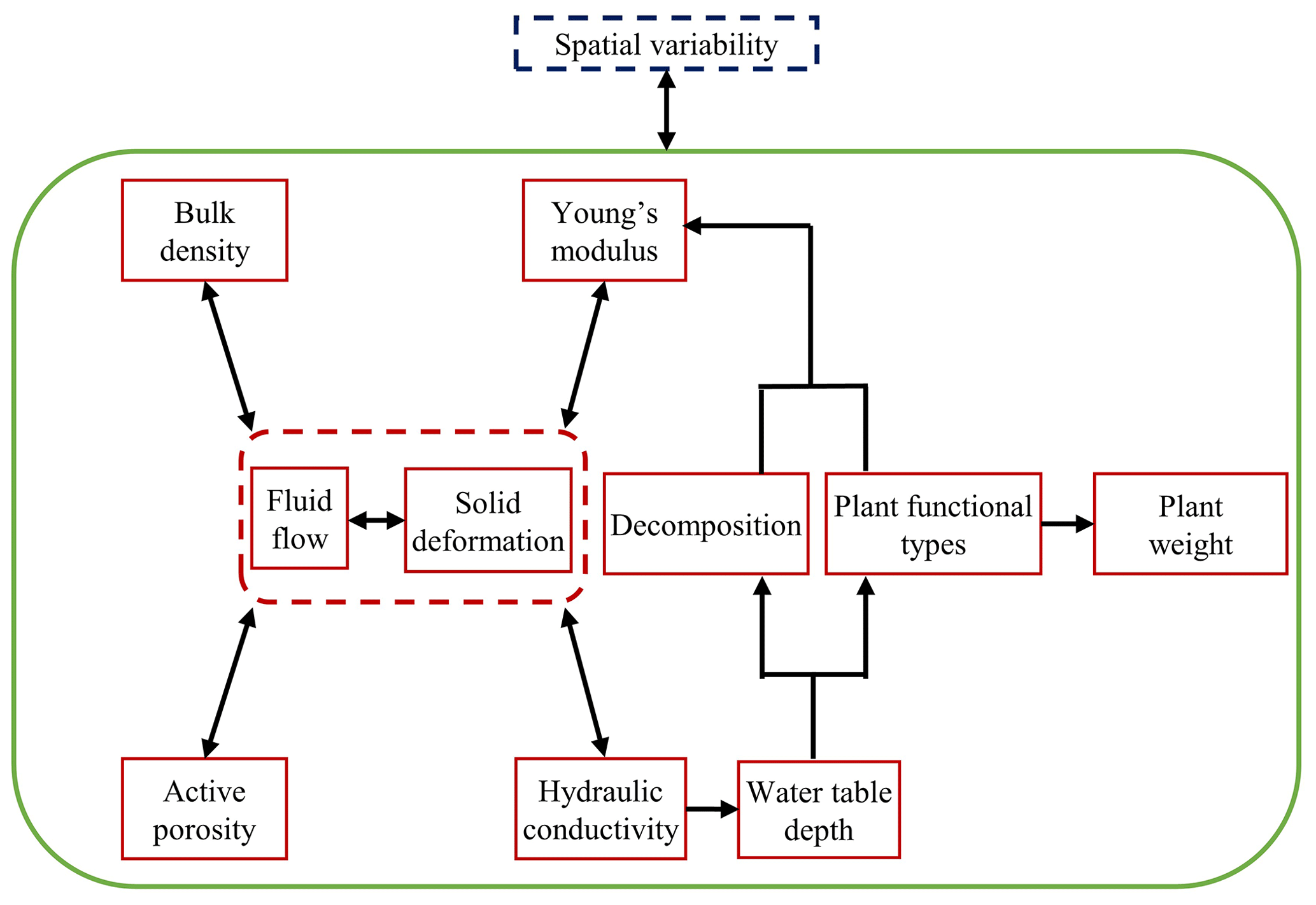
Figure 1 Illustrative formulation of MPeat2D that involves mechanical, ecological, and hydrological processes, together with the feedback from spatial variability on the peatland under a single mathematical and numerical framework.

2.1 Mechanical submodel

The mechanical deformation on the peat body is influenced by the stiffness of the peat solid skeleton and the behaviour of the pore fluid. Reeve et al. (2013) found that a higher value of Young's modulus, which represents the stiffness of the material, leads to a lower deformation effect on the peat body. Furthermore, the characteristics of fluid contained in the peat pore space, including gas content and degree of saturation, also significantly affect the deformation due to the presence of pore fluid pressure (Boylan et al., 2008; Price and Schlotzhauer, 1999; Price, 2003). Therefore, the mechanical submodel is developed based on the poroelasticity theory, which couples solid deformation and fluid flow.

We employ a fully saturated poroelasticity in 2D (Biot, 1941) to model the saturated zone of the peatland below the water table with the governing equations as follows. The equation of equilibrium can be formulated by considering the stress tensor acting on a small elementary area, as written below:

$$\begin{array}{}\text{(1)}& {\stackrel{\mathrm{‾}}{\mathbf{\nabla }}}^{\mathrm{T}}\mathit{\sigma }+\mathit{b}=\mathrm{0},\end{array}$$

with $\stackrel{\mathrm{‾}}{\mathbf{\nabla }}=\left[\begin{array}{cc}\frac{\partial }{\partial x}& \mathrm{0}\\ \mathrm{0}& \frac{\partial }{\partial y}\\ \frac{\partial }{\partial y}& \frac{\partial }{\partial x}\end{array}\right]$, and $\mathit{b}={\left[\begin{array}{cc}\mathrm{0}& \left({\mathit{\rho }}_{\mathrm{w}}\mathit{\varphi }+\mathit{\rho }(\mathrm{1}-\mathit{\varphi })\right)g\end{array}\right]}^{\mathrm{T}}$. In this formulation, $\mathit{\sigma }=[{\mathit{\sigma }}_{xx},{\mathit{\sigma }}_{yy},{\mathit{\sigma }}_{xy}{]}^{\mathrm{T}}$ is the total stress tensor (Pa), b is the body force (N m⁻³), ρ_w is the water density (kg m⁻³), ρ is the peat bulk density (kg m⁻³), ϕ is the active porosity (–), and g is the acceleration in the gravity (m s⁻²). The presentation in terms of matrix form provides a convenient notation for the derivation of the weak form and numerical calculation (Jha and Juanes, 2014).

The stresses on the peat body are distributed to the solid skeleton and pore fluid, resulting in solid displacement and pore fluid pressure. The stress associated with solid displacement is known as effective stress, and it is defined as

$$\begin{array}{}\text{(2)}& {\mathit{\sigma }}^{\mathbf{\prime }}=\mathit{\sigma }-\mathit{\alpha }\mathit{m}p,\end{array}$$

where ${\mathit{\sigma }}^{\mathbf{\prime }}=[{\mathit{\sigma }}_{xx}^{\prime },{\mathit{\sigma }}_{yy}^{\prime },{\mathit{\sigma }}_{xy}^{\prime }{]}^{\mathrm{T}}$ is the effective stress tensor (Pa), $\mathit{\sigma }=[{\mathit{\sigma }}_{xx},{\mathit{\sigma }}_{yy},{\mathit{\sigma }}_{xy}{]}^{\mathrm{T}}$ is the total stress tensor (Pa), α is Biot's coefficient, $\mathit{m}={\left[\begin{array}{ccc}\mathrm{1}& \mathrm{1}& \mathrm{0}\end{array}\right]}^{\mathrm{T}}$, is the vector form of Kronecker's delta, and p is the pore water pressure (Pa). The linear constitutive law gives the relation between effective stress tensor and strain tensor through the following equation:

$$\begin{array}{}\text{(3)}& {\mathit{\sigma }}^{\mathbf{\prime }}=\mathbf{D}\mathit{ϵ},\end{array}$$

with $\mathbf{D}={\displaystyle \frac{E}{(\mathrm{1}+\mathit{\nu })(\mathrm{1}-\mathrm{2}\mathit{\nu })}}\left[\begin{array}{ccc}\mathrm{1}-\mathit{\nu }& \mathit{\nu }& \mathrm{0}\\ \mathit{\nu }& \mathrm{1}-\mathit{\nu }& \mathrm{0}\\ \mathrm{0}& \mathrm{0}& \frac{\mathrm{1}-\mathrm{2}\mathit{\nu }}{\mathrm{2}}\end{array}\right]$. In this formulation ${\mathit{\sigma }}^{\mathbf{\prime }}=[{\mathit{\sigma }}_{xx}^{\prime },{\mathit{\sigma }}_{yy}^{\prime },{\mathit{\sigma }}_{xy}^{\prime }{]}^{\mathrm{T}}$ is the effective stress tensor (Pa), E is Young's modulus (Pa), ν is Poisson's ratio (–), and $\mathit{ϵ}=[{\mathit{ϵ}}_{xx},{\mathit{ϵ}}_{yy},{\mathit{ϵ}}_{xy}{]}^{\mathrm{T}}$ is the strain tensor (–). The relation between strain tensor and displacement provided by the kinematics relations reads

$$\begin{array}{}\text{(4)}& \mathit{ϵ}=\stackrel{\mathrm{‾}}{\mathbf{\nabla }}\mathit{u},\end{array}$$

where $\mathit{ϵ}=[{\mathit{ϵ}}_{xx},{\mathit{ϵ}}_{yy},{\mathit{ϵ}}_{xy}{]}^{\mathrm{T}}$ is the strain tensor (–), and $\mathit{u}=[u_x,u_y{]}^{\mathrm{T}}$ is the displacement (m). Finally, to complete the governing equations of the mechanical submodel, we employ the conservation of mass for solid and fluid constituents. By assuming that water flow in the peat pore space follows Darcy's law and that the volumetric strain is the sum of linear strains, we can formulate the relation between solid deformation, pore water pressure, and the water flow in the peat pore space as

$$\begin{array}{}\text{(5)}& \mathit{\alpha }{\displaystyle \frac{\partial \mathit{ϵ}}{\partial t}}+S_{\mathrm{S}}{\displaystyle \frac{\partial p}{\partial t}}=\mathrm{\nabla }\cdot \left(\mathit{\kappa }\mathrm{\nabla }p\right),\end{array}$$

where α is Biot's coefficient (–), $\mathit{ϵ}={\mathit{ϵ}}_{xx}+{\mathit{ϵ}}_{yy}$ is the volumetric strain (–), S_s is the specific storage (m⁻¹), p is the pore water pressure (Pa), and κ is the hydraulic conductivity (m s⁻¹).

In the unsaturated zone above the water table, we assume that the air pressure is equal to the atmospheric pressure because the water table depth is usually less than 0.5 m in the peatland (Ballard et al., 2011; Swinnen et al., 2019; Mahdiyasa et al., 2022). Consequently, we can expand Eq. (5) to model the unsaturated zone by introducing parameters α_w and M_w that depend on the degree of saturation of water as follows (Cheng, 2020):

$$\begin{array}{}\text{(6)}& {\mathit{\alpha }}_{\mathrm{w}}{\displaystyle \frac{\partial \mathit{ϵ}}{\partial t}}+{\displaystyle \frac{\mathrm{1}}{M_{\mathrm{w}}}}{\displaystyle \frac{\partial p}{\partial t}}=\mathrm{\nabla }\cdot \left(\mathit{\kappa }\mathrm{\nabla }p\right),\end{array}$$

with α_w=S_w, and $M_{\mathrm{w}}=\frac{{\mathit{\gamma }}_{\mathrm{w}}(\mathrm{1}-\mathit{\lambda })}{\mathit{\varphi }\mathit{\lambda }\mathit{\mu }}{S}_{\mathrm{w}}^{-\mathrm{1}/\mathit{\lambda }}(\mathrm{1}-S_{\mathrm{w}}^{\mathrm{1}/\mathit{\lambda }}{)}^{\mathit{\lambda }}$. In this formulation, $\mathit{ϵ}={\mathit{ϵ}}_{xx}+{\mathit{ϵ}}_{yy}$ is the volumetric strain (–), p is the pore water pressure (Pa), κ is the hydraulic conductivity (m s⁻¹), S_w is the degree of saturation of water (–), γ_w is the specific weight of water (N m³), ϕ is the active porosity (–), λ is the first water retention empirical constant (–), and μ is the second water retention empirical constant (m⁻¹).

The discretisation is required in order to solve the partial differential equations from poroelasticity formulation. In 1D, the discretisation is relatively simple because it is conducted over a vertically oriented domain, the length of which represents the height of a peatland (Mahdiyasa et al., 2023, 2022). However, in 2D, the discretisation becomes more complex and is carefully done to circumvent numerical instabilities (Frey and George, 2000; Edelsbrunner, 2001; Zhu et al., 2006). We implement the Delaunay triangulation which provides an optimal and non-overlapping connection between the neighbouring triangles from the data sets of points to create a 2D mesh (Shewchuk, 2002). The Delaunay triangulation does not require a predetermined equation for domain descriptions, which is relevant for our model because the internal and external feedback mechanisms influence the shape and domain of the peatland during the development process.

The peat stiffness, represented by Young's modulus, is modelled as a function of decomposition (Zhu et al., 2020) and plant functional types (PFTs) (Whittington et al., 2007), following the formulation from Mahdiyasa et al. (2023):

$$\begin{array}{}\text{(7)}& E=\mathit{\chi }(\mathrm{1}+{\mathit{\theta }}_t^{\mathit{\zeta }})(b_{\mathrm{1}}{c}_{\mathrm{1}}+b_{\mathrm{2}}{c}_{\mathrm{2}}+b_{\mathrm{3}}{c}_{\mathrm{3}}),\end{array}$$

where E is Young's modulus (Pa); χ is the first Young modulus parameter (Pa); ζ is the second Young modulus parameter (–); θ is the remaining mass (–); $b_{\mathrm{1}},b_{\mathrm{2}},b_{\mathrm{3}}$ are the coefficients to couple PFTs with Young's modulus (–); and $c_{\mathrm{1}},c_{\mathrm{2}},c_{\mathrm{3}}$ are the PFT proportions (–) with the indices $\mathrm{1},\mathrm{2},\mathrm{3}$ indicating shrub, sedge, and Sphagnum, respectively. The interactions between peat stiffness and the load from plant weight, new layer addition, and body force determine the vertical and horizontal displacement of peat solid particles, which affects the bulk density and active porosity due to the changes in the peat volume. We propose the influence of solid displacement on the peat bulk density and active porosity in 2D as follows:

$$\begin{array}{}\text{(8)}& {\displaystyle }{\mathit{\rho }}_t={\displaystyle \frac{{\mathit{\rho }}_{t-\mathrm{1}}}{\mathrm{1}+{\mathit{\beta }}_{\mathit{\rho }}\mathrm{\nabla }\cdot \mathit{u}}},\text{(9)}& {\displaystyle }{\mathit{\varphi }}_t={\displaystyle \frac{{\mathit{\varphi }}_{t-\mathrm{1}}+{\mathit{\beta }}_{\mathit{\varphi }}\mathrm{\nabla }\cdot \mathit{u}}{\mathrm{1}+\mathrm{\nabla }\cdot \mathit{u}}},\end{array}$$

where ρ is the bulk density (kg m⁻³), β_ρ is the bulk density parameter (–), ϕ is the active porosity (–), β_ϕ is the active porosity parameter (–), and $\mathit{u}=[u_x,u_y{]}^{\mathrm{T}}$ is the displacement (m).

2.2 Ecological submodel

We use the formulation from Morris et al. (2015) for the peat production model, which is written as

$$\begin{array}{c}\text{(10)}& {\displaystyle }\begin{array}{rl}{\displaystyle }\mathit{\psi }=& {\displaystyle }\mathrm{0.001}(\mathrm{9.3}+\mathrm{133}z-\mathrm{0.022}(\mathrm{100}z{)}^{\mathrm{2}}{)}^{\mathrm{2}}\\ {\displaystyle }& {\displaystyle }\times (\mathrm{0.1575}\text{Temp}+\mathrm{0.0091}),\text{for}\mathrm{0}\le z\le \mathrm{0.668},\end{array}{\displaystyle }\mathit{\psi }=\mathrm{0},\text{for}z>\mathrm{0.668},\end{array}$$

where ψ is the peat production ($\mathrm{kg}{\mathrm{m}}^{-\mathrm{2}}{\mathrm{yr}}^{-\mathrm{1}}$), z is the water table depth (m), and Temp is the air temperature (°C). Although the peat production model in Eq. (10) has a limitation related to the vegetation composition, this model can couple the ecological and hydrological processes through the dependency between peat production and water table depth. It also includes the effect of air temperature, which leads to a more realistic model. Another approach to model peat production is through the global Thornthwaite Memorial equation (Lieth, 1975) that simulates the primary productivity of the world. However, this model might omit the unique characteristics and the important feedback from the peatland ecosystem that could lead to different estimation of productivity.

Peat production and the PFT proportion are employed to model the plant weight at the top surface through the following equation (Mahdiyasa et al., 2023, 2022; Moore et al., 2002):

$$\begin{array}{}\text{(11)}& {\displaystyle }\begin{array}{rl}{\displaystyle }\mathrm{{\rm Y}}=& {\displaystyle }{c}_{\mathrm{1}}\left({\mathrm{10}}^{\frac{{\log }_{\mathrm{10}}\left(\mathit{\psi }\right)+\mathrm{0.409}}{\mathrm{0.985}}}\right)(\mathrm{1}+d_{\mathrm{1}})g\\ {\displaystyle }& {\displaystyle }+c_{\mathrm{2}}\left({\mathrm{10}}^{{\log }_{\mathrm{10}}\left(\mathit{\psi }\right)+\mathrm{0.001}}\right)(\mathrm{1}+d_{\mathrm{2}})g\\ {\displaystyle }& {\displaystyle }+\left(c_{\mathrm{3}}\mathrm{0.144}\right)(\mathrm{1}+d_{\mathrm{3}})g,\end{array}\end{array}$$

where Υ is the plant weight (Pa); ψ is the peat production ($\mathrm{kg}{\mathrm{m}}^{-\mathrm{2}}{\mathrm{yr}}^{-\mathrm{1}}$); g is the acceleration in the gravity (m s⁻²); $c_{\mathrm{1}},c_{\mathrm{2}},c_{\mathrm{3}}$ are the PFT proportions (–); and $d_{\mathrm{1}},d_{\mathrm{2}},d_{\mathrm{3}}$ are the constants for plant wet condition (–) with the indices $\mathrm{1},\mathrm{2},\mathrm{3}$ indicating shrub, sedge, and Sphagnum, respectively. The proportions of PFTs vary, depending on the position of the water table, with the shrub becoming the dominant PFTs in the low water table condition (Moore et al., 2002; Potvin et al., 2015; Kettridge et al., 2015). Therefore, we use a linear regression model from Mahdiyasa et al. (2023), which was developed from the Moore et al. (2002) data, to model the relationship between PFT proportions with the water table as

$$\begin{array}{}\text{(12)}& {\displaystyle }{c}_{\mathrm{1}}=\mathrm{2.23}z-\mathrm{0.28},\text{(13)}& {\displaystyle }{c}_{\mathrm{2}}=-\mathrm{1.42}z+\mathrm{0.63},\text{(14)}& {\displaystyle }{c}_{\mathrm{3}}=-\mathrm{0.81}z+\mathrm{0.64},\end{array}$$

where $c_{\mathrm{1}},c_{\mathrm{2}},c_{\mathrm{3}}$ are the PFT proportions (–) with the indices 1, 2, and 3 indicating shrub, sedge, and Sphagnum, respectively; z is the water table depth (m). We assign the minimum value of each PFT proportion equal to zero if the value is negative, and we normalise the total proportion.

The decomposition processes occur in the saturated and unsaturated zones of the peatland at different rates. In the saturated zone below the water table, the rate of decay is low due to anoxic conditions, while in the unsaturated zone above the water table, the rate of decay is significantly higher as a consequence of oxic conditions that support the decomposition processes. We follow the model from Clymo (1984) to calculate the changes in peat mass due to the decomposition:

$$\begin{array}{}\text{(15)}& {\displaystyle \frac{\mathrm{d}m}{\mathrm{d}t}}=-\mathit{\eta }m,\end{array}$$

where m is the mass per unit area (kg m⁻²), and η is the rate of decay (yr⁻¹). We do not include the influence of temperature and recalcitrance in the decomposition model because they will increase the number of empirical parameters and assumptions, which might lead to a higher uncertainty in the model. The effect of temperature on the decomposition process could be employed through Q₁₀ parameter (Morris et al., 2015). However, this parameter has a high range of values between 1 and 10 which depends on the peatland types (Xiang and Freeman, 2009; Hardie et al., 2011). Moreover, the inclusion of the recalcitrance effect requires additional assumptions related to the changes in the rate of decay that could follow a range of models, as shown by Clymo et al. (1998).

The effect of decomposition is represented as the remaining mass, which is defined as the ratio between mass at time t, which has experienced decay and the initial mass (Mahdiyasa et al., 2022; Baird et al., 2012; Morris et al., 2012, 2015).

$$\begin{array}{}\text{(16)}& {\mathit{\theta }}_t={\displaystyle \frac{m_t}{m_{\mathrm{0}}}},\end{array}$$

where θ is the remaining mass (–), m_t is the mass per unit area at time t (kg m⁻²), and m₀ is the initial mass per unit area (kg m⁻²).

2.3 Hydrological submodel

We model the peatland groundwater flows in 2D using the Boussinesq equation subject to net rainfall that acts as a source term (Cobb et al., 2017; Baird et al., 2012; Morris et al., 2012).

$$\begin{array}{}\text{(17)}& S_{\mathrm{y}}{\displaystyle \frac{\partial W}{\partial t}}=\mathrm{\nabla }\cdot \left(T\mathrm{\nabla }W\right)+r,\end{array}$$

where W is the water table height (m), S_y is the specific yield (–), T is the transmissivity (m² yr⁻¹), and r is the net rainfall (m yr⁻¹) that is defined as precipitation minus evapotranspiration. The Boussinesq equation is based on the Dupuit and Forchheimer (D–F) assumption (Bartlett and Porporato, 2018) which states that groundwater flows horizontally in unconfined aquifers. The D–F assumption is appropriate to model peatland groundwater flow because the peatland lateral distance is much wider than the thickness, which leads to the dominant horizontal flow. We assume that the height of the water table cannot surpass the height of the peatland because the water will flow as surface water (Mahdiyasa et al., 2022; Morris et al., 2011). This would appear to be a realistic assumption because we do not simulate patterned peatlands. Consequently, the water table depth is obtained from the difference between peatland height and water table height as follows:

$$\begin{array}{}\text{(18)}& z=h-W,\end{array}$$

where z is the water table depth (m), h is the peatland height (m), and W is the water table height (m).

The mechanical deformation changes the peat pore structure, leading to variations in the active porosity (Eq. 9) and influencing water flow through the pore space. Therefore, we implement the hydraulic conductivity model from Mahdiyasa et al. (2022), who formulate the changes in hydraulic conductivity as a function of active porosity.

$$\begin{array}{}\text{(19)}& {\mathit{\kappa }}_t={\mathit{\kappa }}_{\mathrm{0}}{\left({\displaystyle \frac{{\mathit{\varphi }}_t}{{\mathit{\varphi }}_{\mathrm{0}}}}\right)}^{\mathit{\xi }},\end{array}$$

where κ is the hydraulic conductivity (m s⁻¹), κ₀ is the initial value of hydraulic conductivity (m s⁻¹), ϕ is the active porosity (–), ϕ₀ is the initial value of active porosity (–), and ξ is the hydraulic conductivity parameter (–). Compared to the hydraulic conductivity model developed by Morris et al. (2022) from the meta-analysis of northern peat samples, Eq. (19) provides a more straightforward approach to analyse the influence of mechanical deformation on peatland hydrology because the active porosity and hydraulic conductivity are a function of solid displacement.

2.4 Numerical verification

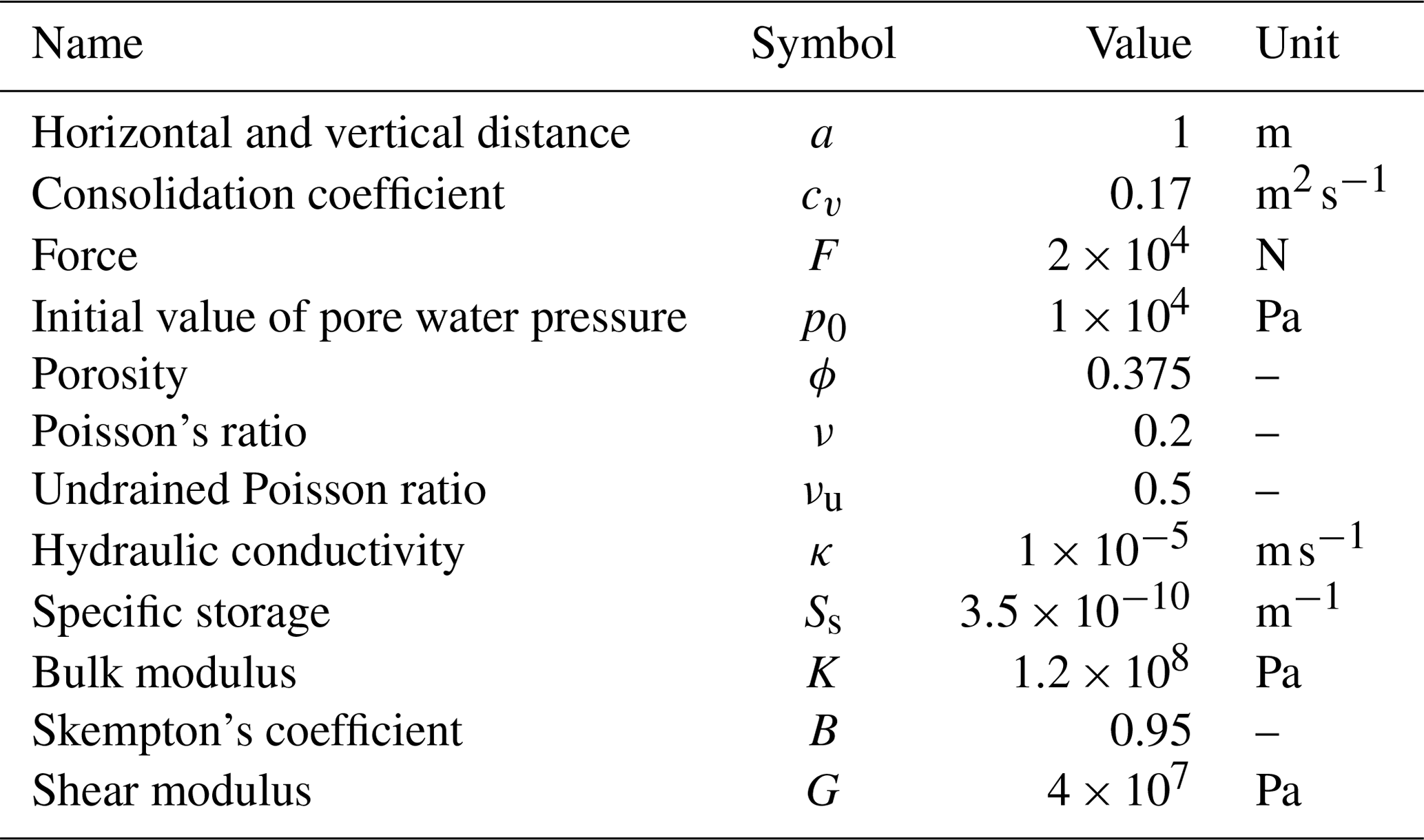
The verification is focused on the mechanical submodel, particularly the poroelasticity formulation, by comparing numerical calculations with analytical solutions from Mandel's problem (Mandel, 1953). Uniform vertical load 2F is applied to a rectangular sample through a rigid and frictionless plate of width 2a and height 2H, with drainage to the two sides in the lateral condition, as shown in Fig. 2. The deformation of the sample is forced to be an in-plane strain condition by preventing all deformation in the direction perpendicular to the plane. The pore water pressure distribution will be homogeneous at the instant loading, but when drainage starts, the pore water pressure at two sides, $x=-a$ and x=a, is reduced to zero and followed by the pore water pressure in the interior. Because the discharge has only a horizontal component, the pore water pressure, stress, and strain are independent of the y coordinate. Furthermore, σ_xx=0, σ_xy=0, u_x is independent of y, and u_y is independent of x. Since the problem is symmetric, we solve only the upper-right quadrant of the xy plane. We use 441 nodes and 800 elements to generate the simulations. The data for analytical and numerical solutions of this problem are stated in Table 1.

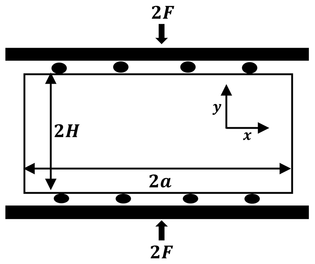
Figure 2 The illustration of Mandel's problem for the two-dimensional poroelasticity verification.

Table 1 Input data for numerical and analytical solutions of Mandel's problem.

The analytical solutions to Mandel's problem for the pore water pressure and horizontal and vertical displacement are (Cheng and Detournay, 1988; Abousleiman et al., 1996; Phillips and Wheeler, 2007)

$$\begin{array}{}\text{(20)}& {\displaystyle }\begin{array}{rl}{\displaystyle }p=& {\displaystyle \frac{\mathrm{2}FB(\mathrm{1}+{\mathit{\nu }}_{\mathrm{u}})}{\mathrm{3}a}}{\sum }_{i=\mathrm{1}}^{\mathrm{\infty }}{\displaystyle \frac{\sin {\mathit{\omega }}_i}{{\mathit{\omega }}_i-\sin {\mathit{\omega }}_i\cos {\mathit{\omega }}_i}}\\ {\displaystyle }& {\displaystyle }\times \left(\cos {\displaystyle \frac{{\mathit{\omega }}_{i}x}{a}}-\cos {\mathit{\omega }}_i\right)\exp \left(-{\displaystyle \frac{{\mathit{\omega }}_i^{\mathrm{2}}{c}_{v}t}{a^{\mathrm{2}}}}\right),\end{array}\text{(21)}& {\displaystyle }\begin{array}{rl}{\displaystyle }{u}_x=& {\displaystyle }\left[{\displaystyle \frac{F\mathit{\nu }}{\mathrm{2}Ga}}-{\displaystyle \frac{F{\mathit{\nu }}_{\mathrm{u}}}{Ga}}{\sum }_{i=\mathrm{1}}^{\mathrm{\infty }}{\displaystyle \frac{\sin {\mathit{\omega }}_i\cos {\mathit{\omega }}_i}{{\mathit{\omega }}_i-\sin {\mathit{\omega }}_i\cos {\mathit{\omega }}_i}}\exp \left(-{\displaystyle \frac{{\mathit{\omega }}_i^{\mathrm{2}}{c}_{v}t}{a^{\mathrm{2}}}}\right)\right]x\\ {\displaystyle }& {\displaystyle }+{\displaystyle \frac{F}{G}}{\sum }_{i=\mathrm{1}}^{\mathrm{\infty }}{\displaystyle \frac{\cos {\mathit{\omega }}_i}{{\mathit{\omega }}_i-\sin {\mathit{\omega }}_i\cos {\mathit{\omega }}_i}}\sin {\displaystyle \frac{{\mathit{\omega }}_{i}x}{a}}\exp \left(-{\displaystyle \frac{{\mathit{\omega }}_i^{\mathrm{2}}{c}_{v}t}{a^{\mathrm{2}}}}\right),\end{array}\text{(22)}& {\displaystyle }\begin{array}{rl}{\displaystyle }{u}_y=& {\displaystyle }\left[-{\displaystyle \frac{F(\mathrm{1}-\mathit{\nu })}{\mathrm{2}Ga}}+{\displaystyle \frac{F(\mathrm{1}-{\mathit{\nu }}_{\mathrm{u}})}{Ga}}{\sum }_{i=\mathrm{1}}^{\mathrm{\infty }}{\displaystyle \frac{\sin {\mathit{\omega }}_i\cos {\mathit{\omega }}_i}{{\mathit{\omega }}_i-\sin {\mathit{\omega }}_i\cos {\mathit{\omega }}_i}}\right.\\ {\displaystyle }& {\displaystyle }\left.\times \exp \left(-{\displaystyle \frac{{\mathit{\omega }}_i^{\mathrm{2}}{c}_{v}t}{a^{\mathrm{2}}}}\right)\right]y,\end{array}\end{array}$$

with $\tan {\mathit{\omega }}_i=\frac{\mathrm{1}-\mathit{\nu }}{{\mathit{\nu }}_{\mathrm{u}}-\mathit{\nu }}{\mathit{\omega }}_i$. In this analytical solution, p is the pore water pressure (Pa), u_x is the horizontal displacement (m), u_y is the vertical displacement (m), F is the force (N), B is Skempton's coefficient (–), G is the shear modulus (Pa), ν is Poisson's ratio (–), and ν_u is the undrained Poisson ratio (–).

The comparison between numerical and analytical solutions for Mandel's problem for normalised pore water pressure, normalised horizontal displacement, and normalised vertical displacement is shown in Fig. 3 at various dimensionless times $t^{\ast }=c_{v}t/a^{\mathrm{2}}$. The mean absolute errors for normalised pore water pressure and displacement are small. The first variable, normalised pore water pressure, has a mean absolute error of around $\mathrm{3.8}\times {\mathrm{10}}^{-\mathrm{3}}$, $\mathrm{3.7}\times {\mathrm{10}}^{-\mathrm{4}}$, and $\mathrm{5.2}\times {\mathrm{10}}^{-\mathrm{6}}$ at dimensionless time equal to 0.01, 0.1, and 0.5, respectively. For the second variable, normalised horizontal displacement, has a mean absolute error of around $\mathrm{2.8}\times {\mathrm{10}}^{-\mathrm{3}}$ and $\mathrm{1.4}\times {\mathrm{10}}^{-\mathrm{6}}$ at dimensionless time equal to 0.1 and 0.5, respectively. Finally, the mean absolute error in the normalised vertical displacement is about $\mathrm{1.1}\times {\mathrm{10}}^{-\mathrm{3}}$ at dimensionless time equal to 0.1 and is $\mathrm{5.8}\times {\mathrm{10}}^{-\mathrm{7}}$ at dimensionless time equal to 0.5.

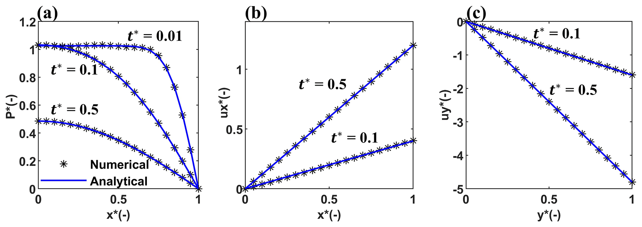
Figure 3 Numerical and analytical solutions of Mandel's problem at various dimensionless time $t^{\ast }=c_{v}t/a^{\mathrm{2}}$ for (a) normalised pore water pressure $P^{\ast }=\frac{p}{p_{\mathrm{0}}}$, (b) normalised horizontal displacement $u_x^{\ast }=\frac{u_x}{u_{x\mathrm{0}}}$, and (c) normalised vertical displacement $u_y^{\ast }=\frac{u_y}{u_{y\mathrm{0}}}$. The initial displacements in the horizontal and vertical directions are obtained from $u_{x\mathrm{0}}=\frac{F{\mathit{\nu }}_{\mathrm{u}}x}{\mathrm{2}Ga}$ and $u_{y\mathrm{0}}=\frac{F(\mathrm{1}-{\mathit{\nu }}_{\mathrm{u}})y}{\mathrm{2}Ga}$, respectively. In this verification, $x^{\ast }=\frac{x}{a}$ is the normalised horizontal distance, and $y^{\ast }=\frac{y}{a}$ is the normalised vertical distance.

Mandel's problem has an interesting characteristic related to the behaviour of pore water pressure. In the centre of the sample, the pore water pressure will be higher than the initial pressure for a small time interval. The value of normalised pore water pressure is greater than one at $t^{\ast }=\mathrm{0.01}$ and $t^{\ast }=\mathrm{0.1}$ (Fig. 3a). This phenomenon is denoted as the Mandel–Cryer effect, and it occurs due to the deformation and rigid plate conditions producing an additional source term for the pore water pressure distribution (Phillips and Wheeler, 2007; van Duijn and Mikelic, 2021).

3 Model implementation

We simulate long-term peatland development over 5000 years with flat, impermeable, and rigid substrates constrained by the parallel rivers at the edges (Ingram, 1982), with the parameter values summarised in Table 2. We assume the rivers do not incise, which could affect the water discharge (Glaser et al., 2004). Therefore, we implement no displacement and no flux boundary conditions at the bottom and zero pore water pressure at the edges. To reduce the computational time, we model half of the peatland domain from the central vertical axis to the one river with a distance of 500 m due to the symmetric growth assumption of the peatland (Baird et al., 2012; Morris et al., 2012). The boundary conditions for the central axis are impermeable without experiencing horizontal displacement.

Table 2 Parameter default values for the simulations.

The total load on this system is associated with the surficial peat addition (Eq. 10), plant weight (Eq. 11), and body force (Eq. 1). The surficial peat addition and plant weight are applied at the surface, while the body force acts throughout the peatland area. The surface loadings are influenced by the peat production and vegetation composition consisting of shrub, sedge, and Sphagnum. Different from the surface loadings that are controlled by external sources, the body force is obtained from peatland self-weight, which is determined by the peat bulk density, water density, and active porosity.

To illustrate how MPeat2D works, we run two groups of simulations with different climate inputs. In the first group, we employ constant net rainfall (0.8 m yr⁻¹) and air temperature (6 °C) to provide the basic simulation related to the influence of mechanical–ecohydrological feedback and spatial heterogeneity of peat physical properties, water table depth, PFT proportion, and plant weight on peatland behaviour (Fig. 4). In the second group, we use a non-constant annual time series of net rainfall and air temperature generated from the sinusoidal function with some noise (Mahdiyasa et al., 2023, 2022) and with the range value of 0.6–1 m yr⁻¹ and 4–7 °C, respectively (Morris et al., 2015; Young et al., 2021, 2019). Through this approach, we can capture the wet and dry climatic influence on the long-term development of peatlands and maintain the simplicity of our climate reconstruction as the input variable.

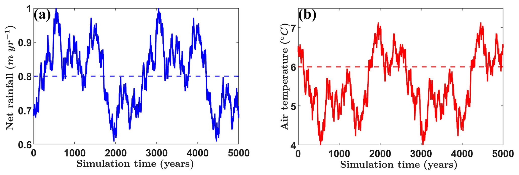
Figure 4 The climate profile for (a) net rainfall and (b) air temperature over 5000 years under constant and non-constant conditions. The values of a constant climate are 0.8 m yr⁻¹ and 6 °C, indicated by dashed lines, while the non-constant climate, specified by continuous lines, fluctuates between 0.6 and 1 m yr⁻¹ for net rainfall and between 4 and 7 °C for air temperature.

We compare the results obtained from MPeat2D with the previously developed mechanical–ecohydrological model of peatland development in 1D called MPeat (Mahdiyasa et al., 2022, 2023) and with the 2D non-poroelastic ecohydrological model of peatland growth called DigiBog (Morris et al., 2012; Baird et al., 2012). The comparison with MPeat is conducted for the water table depth, peatland height, and cumulative carbon from the centre area using the same parameters and climatic influence summarised in Table 2 and Fig. 4, respectively. In both models, cumulative carbon is obtained from cumulative mass multiplied by 47 % of the carbon content (Loisel et al., 2014). The comparison with DigiBog employs the model version provided by Baird et al. (2012) and Morris et al. (2012), which is run under a constant climate with the value of bulk density equal to 100 kg m⁻³ and the hydraulic conductivity parameters a and b equal to $\mathrm{1}\times {\mathrm{10}}^{-\mathrm{5}}$ m s⁻¹ and 8, respectively. We chose this model version of DigiBog because it has similar characteristics to MPeat2D, including the flat and impermeable substrate with the symmetric assumption of peatland growth, and it does not simulate the influence of poroelasticity on the peatland behaviour. This model maintains the annual increments and layer properties without lumping the layers for numerical efficiency into larger averaged layers, which could lead to more stable numerical calculations. The bulk density and active porosity are constant throughout the simulation time, but hydraulic conductivity is allowed to change because of the decomposition process. The peat volume can only change as a result of the mass lost, and there are no volume changes due to the deformation of the peat in this model. Consequently, this model version of DigiBog provides sufficient tests of the effect of removing poroelasticity, while still assuming reasonable values of hydraulic conductivity, bulk density, and active porosity. The output variables from the comparison between MPeat2D and DigiBog are peatland shape in cross section, thickness, and water table depth.

The sensitivity analysis of MPeat2D is conducted by changing the first Young modulus parameter χ to 3.5×10⁵ and 4.5×10⁵ Pa. We performed one-at-a-time sensitivity analysis by focusing on the variation in one parameter, and we set all other parameters to remain the same as the baseline value (Table 2). The first Young modulus parameter χ is chosen because it determines the peat stiffness, which in turn influences the mechanical deformation of the peat body. Output variables examined from the sensitivity analysis include the spatial variations in bulk density, active porosity, and hydraulic conductivity.

4 Simulation results

4.1 First group: constant climate

In the initial stage of development, the peatland shape is relatively flat, with a low value of bulk density and a high value of active porosity and hydraulic conductivity. By 5000 years, a dome-shaped peatland is produced, with the maximum thickness obtained at the centre and decreasing toward the margin. The increasing thickness leads to higher loading and a more significant deformation effect on the peat pore structure, which affects the peat physical properties. The changes in peat physical properties during the development process exhibit spatial variabilities in the vertical and horizontal directions with the range of values between 50 and 100 kg m⁻³, 0.49 and 0.8, and $\mathrm{5.5}\times {\mathrm{10}}^{-\mathrm{6}}$ and $\mathrm{1}\times {\mathrm{10}}^{-\mathrm{2}}$ m s⁻¹ for bulk density, active porosity, and hydraulic conductivity, respectively (Fig. 5).

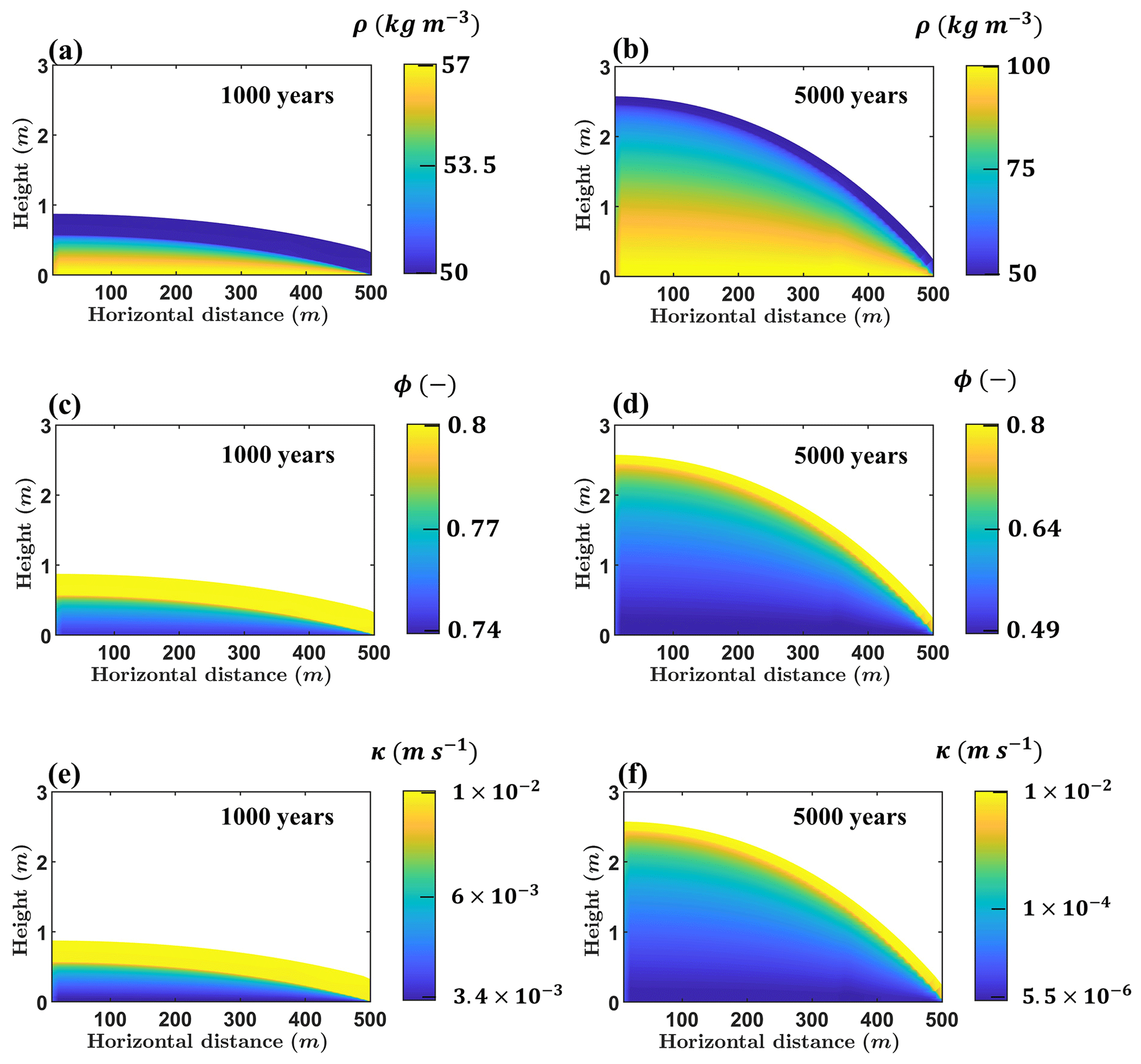
Figure 5 The profiles of (a, b) bulk density, (c, d) active porosity, and (e, f) hydraulic conductivity with spatial variability in the vertical and horizontal directions under a constant climate.

Over 5000 years of development, the water table depth decreases, resulting in the wetter condition of the peatland (Fig. 6). This condition occurs because the loading from peat accumulation increases as the peatland grows, which provides internal feedback mechanisms to the water balance through the deformation of peat pore space. The difference in the final simulation year between the water table depth at the centre (0.13 m) and at the margin (0.20 m), which is separated by a horizontal distance of 500 m, leads to the variation in the vegetation composition and plant weight. The proportion of shrub is lower at the centre compared to the margin, with values of about 1 % and 17 %, respectively. In contrast, the sedge and Sphagnum proportions reduce from around 45 % and 54 % at the centre to 35 % and 48 % at the margin, respectively. The variations in the vegetation composition affect the distribution of plant weight, with the centre (19 kg m⁻²) providing a lower value of loading than the margin (22 kg m⁻²).

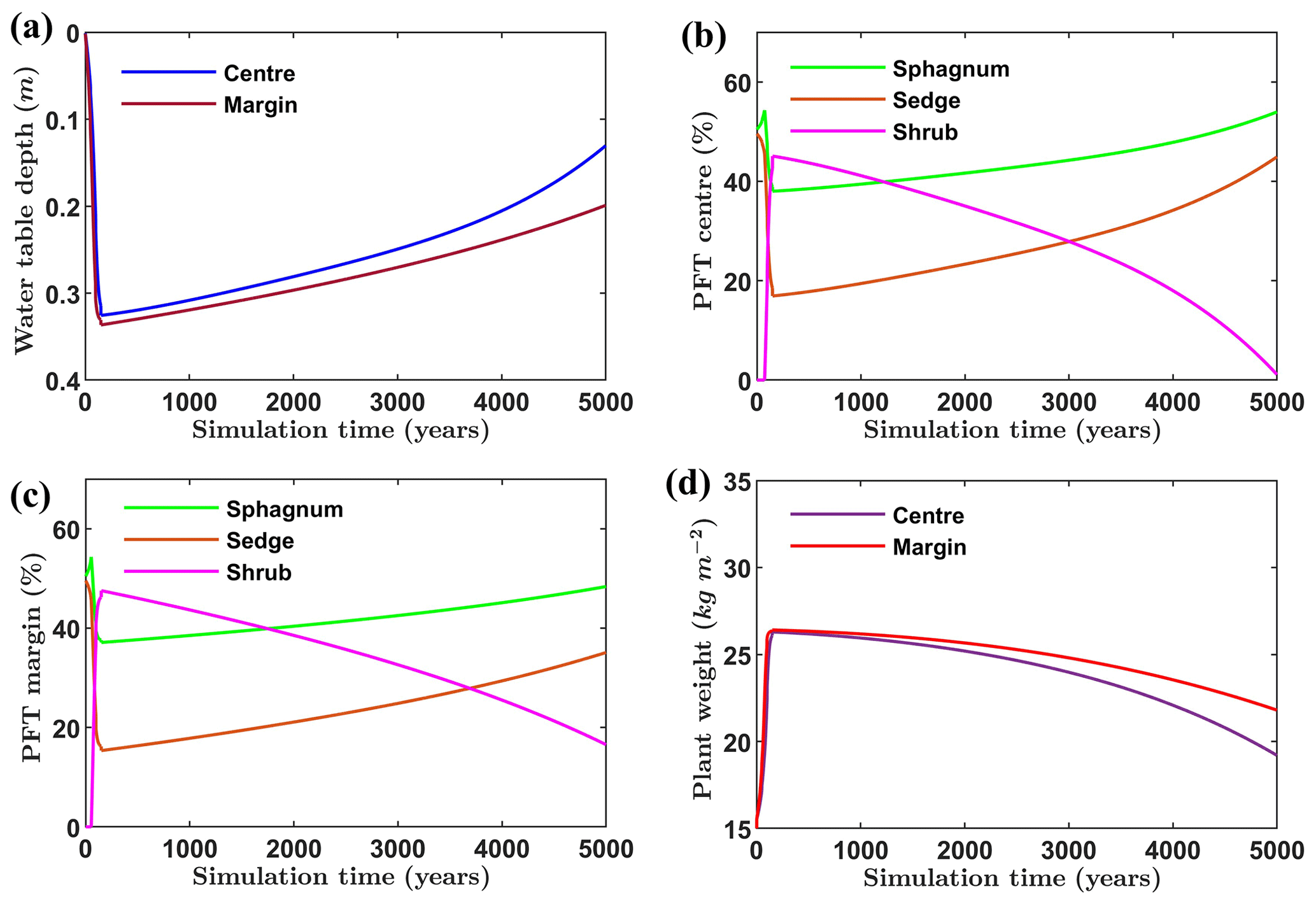
Figure 6 The variations in the (a) water table depth, (b) plant functional type (PFT) proportion at the centre, (c) PFT proportion at the margin, and (d) plant weight over 5000 years under a constant climate. The centre is defined at the central vertical axis, while the margin is located at a horizontal distance of 500 m from the centre.

4.2 Second group: non-constant climate

Under a non-constant climate, the profiles of peat physical properties are similar to those in the constant climate case. The value of bulk density increases while active porosity and hydraulic conductivity decrease from the centre toward the margin (Fig. 7). The main difference is that the range values of bulk density (50–104 kg m⁻³), active porosity (0.47–0.8), and hydraulic conductivity ($\mathrm{3.7}\times {\mathrm{10}}^{-\mathrm{6}}$–$\mathrm{1}\times {\mathrm{10}}^{-\mathrm{2}}$ m s⁻¹) are higher in the second group after 5000 years. This condition indicates a more significant effect of mechanical deformation on the peat pore space due to the changing climate.

Figure 7 The profiles of (a, b) bulk density, (c, d) active porosity, and (e, f) hydraulic conductivity with spatial variability in the vertical and horizontal directions under a non-constant climate.

After the unsaturated zone is developed, around 150 years after peatland initiation, the water table depth experiences fluctuations and exhibits lateral variability. The margin, which is located at a horizontal distance of 500 m from the centre, experiences drier conditions indicated by a higher water table depth compared to the centre (Fig. 8). Furthermore, the spatial variability in the water table depth results in lateral changes in PFT proportions and plant weight. For example, around the year 3750, the water table depth is about 0.07 m at the centre, while at the margin, the water table is located about 0.22 m below the surface. Consequently, the shrub proportion increases from 0 % at the centre to 21 % at the margin, while sedge and Sphagnum decrease from 48 % and 52 % to 32 % and 47 % from the centre to the margin, respectively. This condition produces a spatial variation in plant weight between the centre and the margin with values of about 17 and 22 kg m⁻².

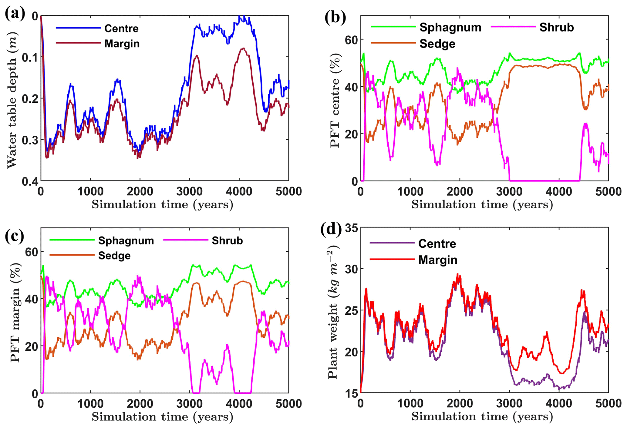
Figure 8 The variations in the (a) water table depth, (b) plant functional type (PFT) proportion at the centre, (c) PFT proportion at the margin, and (d) plant weight over 5000 years under a non-constant climate. The centre is defined at the central vertical axis, while the margin is located at a horizontal distance of 500 m from the centre.

4.3 Comparison among MPeat2D, MPeat, and DigiBog

The comparison between MPeat2D and MPeat is conducted based on the simulation at the centre of the peatland. Under a constant climate, the emergence of the unsaturated zone, represented by the non-zero values of water table depth, is faster in the MPeat2D than in the MPeat, with a difference of about 360 years (Fig. 9a). Moreover, the water table depth obtained from MPeat2D (0.13 m) is lower than MPeat (0.3 m) in the final simulation year. Although MPeat2D and MPeat estimate similar peatland height with values of about 2.57 and 2.52 m (Fig. 9b), respectively, the cumulative carbon obtained from MPeat2D (89 kg C m⁻²) is higher compared to the MPeat (84 kg C m⁻²) over 5000 years (Fig. 9c).

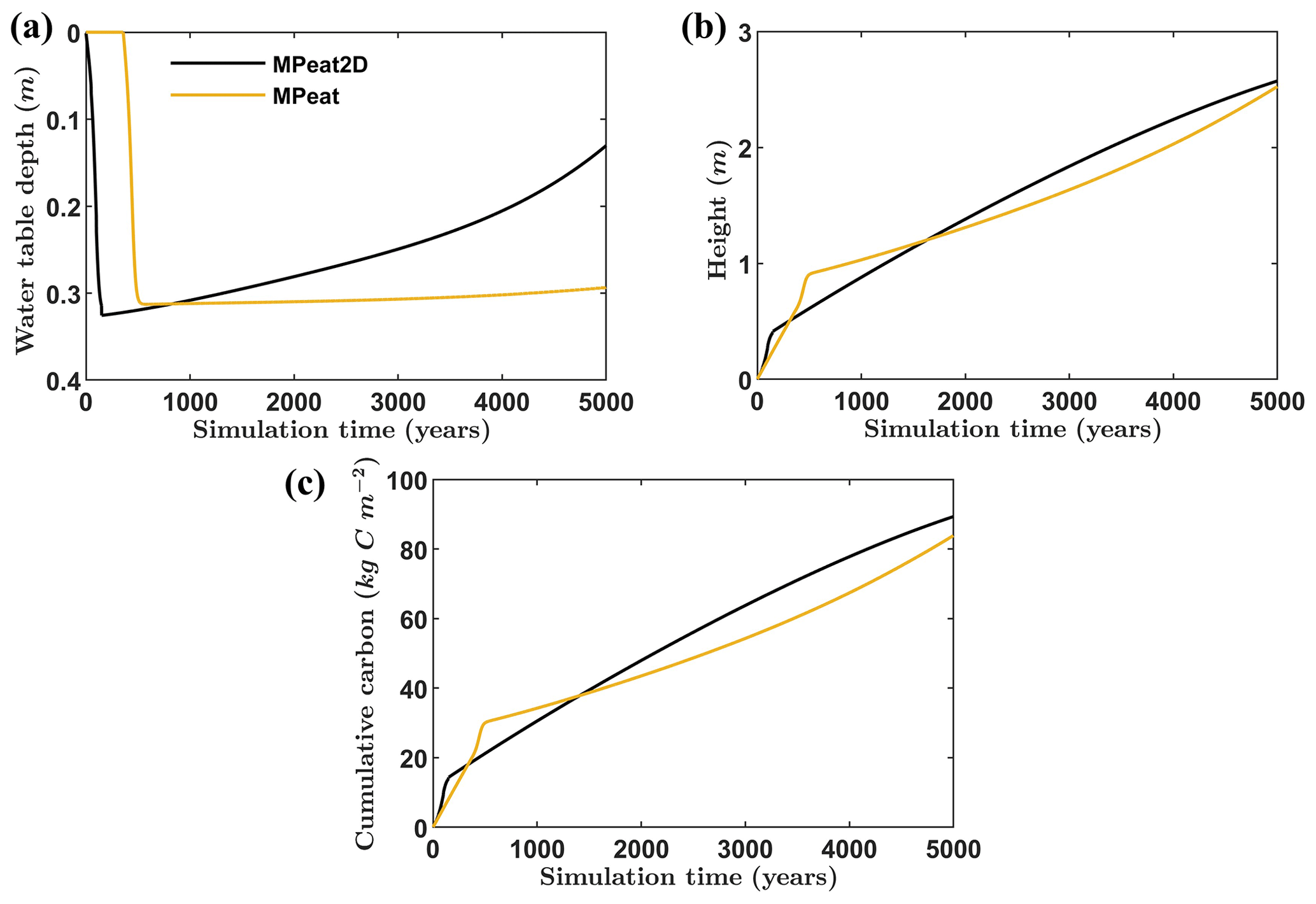
Figure 9 The comparison between MPeat2D and MPeat at the centre for (a) water table depth, (b) peatland height, and (c) cumulative carbon over 5000 years under a constant climate.

The comparisons between MPeat2D and MPeat for water table depth, peatland height, and cumulative carbon at the centre area under a non-constant climate are shown in Fig. 10. The appearance of the unsaturated zone is around 400 years earlier in MPeat2D than MPeat, based on the non-zero values of the water table depth since peatland initiation. After the unsaturated zone is developed in both models, MPeat2D predicts a lower water table depth compared to MPeat with the range value of 0–0.34 m and 0.16–0.36 m, respectively. Peatland height and cumulative carbon obtained from MPeat2D around 2.61 m and 92 kg C m⁻² are more significant than the MPeat-estimated values of about 2.39 m and 76 kg C m⁻² after 5000 years.

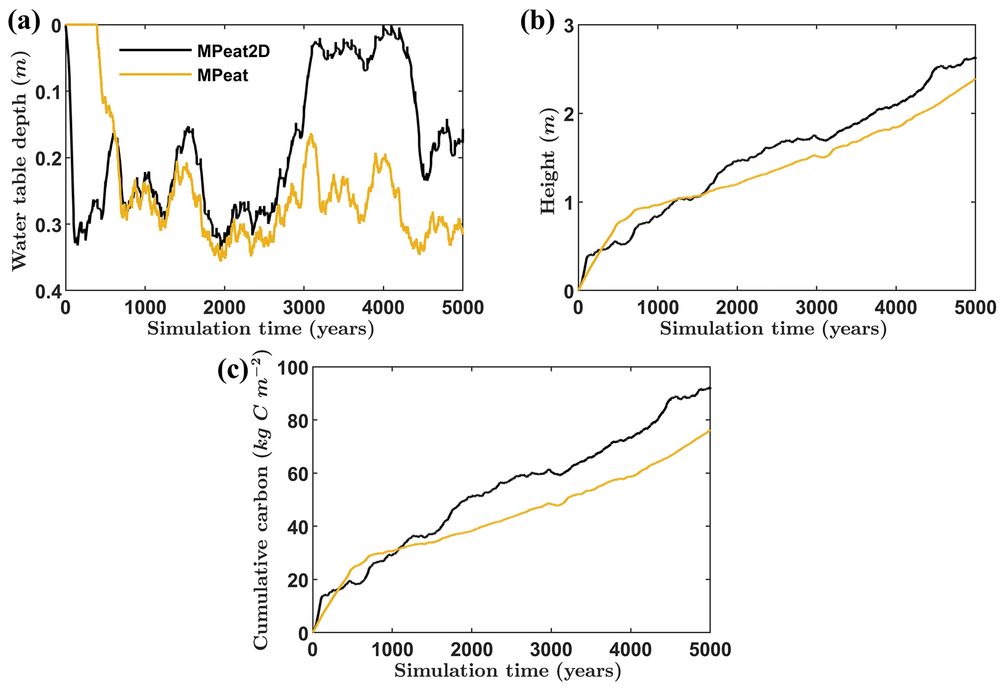
Figure 10 The comparison between MPeat2D and MPeat at the centre for (a) water table depth, (b) peatland height, and (c) cumulative carbon over 5000 years under a non-constant climate.

The comparison between MPeat2D and DigiBog is run only under a constant climate due to the limitations of the chosen DigiBog version (Morris et al., 2012; Baird et al., 2012). Over 5000 years, the peatland height at the centre obtained from MPeat2D is higher compared to DigiBog, with a difference of about 0.6 m (Fig. 11a). Furthermore, both models produce peatland shapes that experience the formation of a cliff at the margin. The heights of the cliffs obtained from MPeat2D and DigiBog are about 0.27 and 1.15 m, respectively. The spatial variations in the water table depth between the centre and the margin are more significant in MPeat2D compared to DigiBog (Fig. 11b). In the final simulation year, MPeat2D simulates the water table depth with values of about 0.13 m at the centre and 0.2 m at the margin, while DigiBog produces a water table depth of around 0.43 and 0.44 m at the centre and margin, respectively.

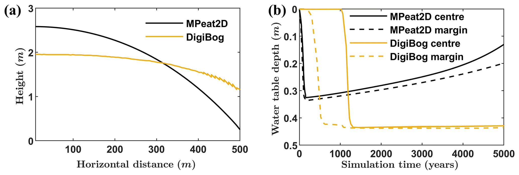
Figure 11 The comparison between MPeat2D and DigiBog Bog 2 (Morris et al., 2012) for the (a) peatland shape and (b) water table depth over 5000 years. Both models assume that the peatland develops above the flat and impermeable substrate with a constant climate.

4.4 Sensitivity analysis

We changed the first peat Young modulus parameter χ, which is an essential variable in the MPeat2D because it determines the peat stiffness and the compaction effect on the peat pore structure. Under a constant climate (Fig. 12), reducing the first peat Young modulus parameter χ to 3.5×10⁵ Pa led to a higher value of the bulk density (50–111 kg m⁻³) and lower values of the active porosity (0.44–0.8) and hydraulic conductivity ($\mathrm{1.2}\times {\mathrm{10}}^{-\mathrm{6}}$–$\mathrm{1}\times {\mathrm{10}}^{-\mathrm{2}}$ m s⁻¹). The more significant effect of compaction due to a lower first peat Young modulus parameter χ results in a decreasing peatland height at the centre by about 6 % compared to the baseline value after 5000 years. Contrastingly, increasing the first peat Young modulus parameter χ to 4.5×10⁵ Pa produced a lower bulk density (50–94 kg m⁻³) and higher active porosity (0.52–0.8) and hydraulic conductivity ($\mathrm{1.6}\times {\mathrm{10}}^{-\mathrm{5}}$–$\mathrm{1}\times {\mathrm{10}}^{-\mathrm{2}}$ m s⁻¹). These conditions increased the peatland height at the centre by about 4 % compared to the baseline value in the final simulation year.

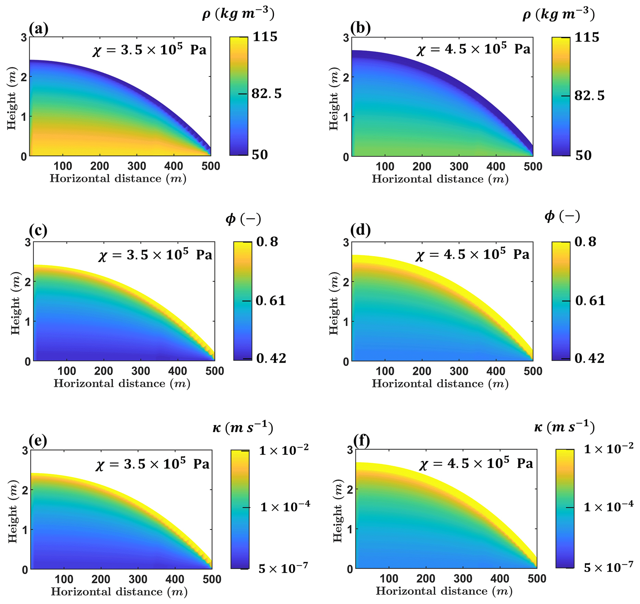
Figure 12 The sensitivity analysis of MPeat2D conducted by changing the first Young modulus parameter χ with the output variables (a, b) bulk density, (c, d) active porosity, and (e, f) hydraulic conductivity under a constant climate over 5000 years. In the base run, χ is equal to 4×10⁵ Pa.

Under a non-constant climate (Fig. 13), the influence of parameter χ on the peat physical properties and thickness is similar to that observed in the constant climate scenario. Reducing χ to 3.5×10⁵ Pa resulted in a higher bulk density (50–114 kg m⁻³) and lower active porosity (0.42–0.8) and hydraulic conductivity ($\mathrm{6.9}\times {\mathrm{10}}^{-\mathrm{7}}$–$\mathrm{1}\times {\mathrm{10}}^{-\mathrm{2}}$ m s⁻¹). As a consequence, the peatland height at the centre was reduced by about 5 % compared to the baseline value after 5000 years. In contrast, increasing χ to 4.5×10⁵ Pa led to a lower bulk density (50–96 kg m⁻³) and higher active porosity (0.51–0.8) and hydraulic conductivity ($\mathrm{1.2}\times {\mathrm{10}}^{-\mathrm{5}}$–$\mathrm{1}\times {\mathrm{10}}^{-\mathrm{2}}$ m s⁻¹), which in turn produced a more significant peatland thickness at the centre by about 4 % compared to the baseline value over 5000 years of simulations.

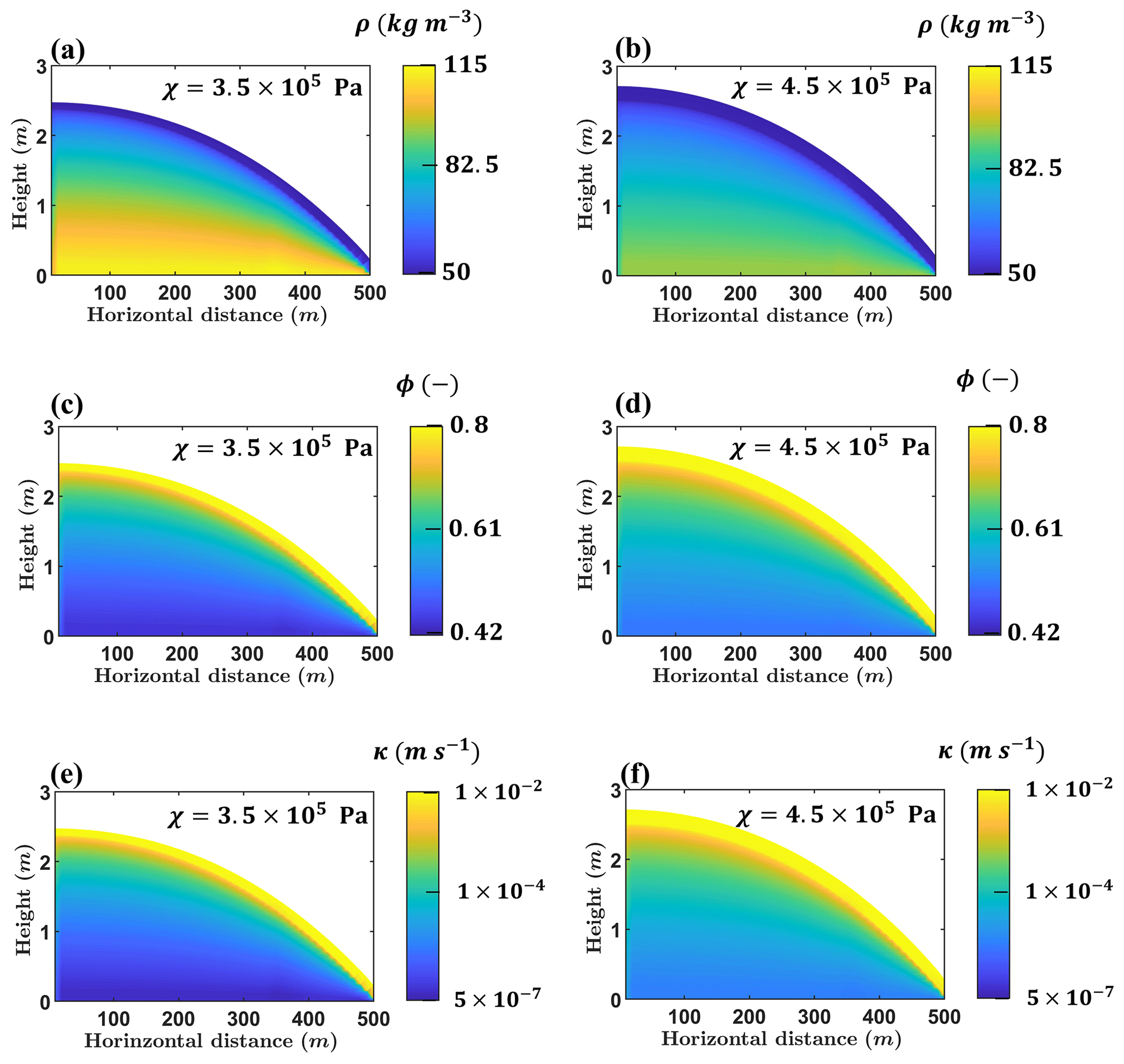
Figure 13 The sensitivity analysis of MPeat2D conducted by changing the first Young modulus parameter χ with the output variables (a, b) bulk density, (c, d) active porosity, and (e, f) hydraulic conductivity under a non-constant climate over 5000 years. In the base run, χ is equal to 4×10⁵ Pa.

5 Discussion

The most important result from MPeat2D is the ability to model the influence of spatial variability on long-term peatland behaviour. The addition of the second dimension provides significant impacts on the analysis of peat physical properties because it allows the bulk density, active porosity, and hydraulic conductivity to change in the horizontal and vertical directions. We found that the bulk density increases systematically from the centre to the margin, while the active porosity and hydraulic conductivity experience an opposite pattern with decreasing values from the peatland interior to the edges (Figs. 5 and 7). The horizontal variability in the peat physical properties is not only caused by different effects of decomposition (Morris et al., 2012) but also by different effects of compaction between the margin and the centre. The steeper hydraulic gradient at the margin promotes water release and reduces the position of the water table (Figs. 6a and 8a) (Reeve et al., 2006; Lewis et al., 2012; Kværner and Snilsberg, 2011; Regan et al., 2019), which results in higher loading from the plant weight (Figs. 6d and 8d) and effective stress. In contrast, peatland topography at the centre is mainly flat, leading to the shallow water table position that limits the deformation of the peat pore space.

At smaller scales of a few metres, another possible factor affecting the horizontal variance in peat physical properties is the peatland microform. The measurement from Whittington and Price (2006) indicated that bulk density and hydraulic conductivity differ substantially in the lateral direction over distances of a few metres between hummocks, lawns, and hollows. Moreover, Baird et al. (2016) showed that the difference in the hydraulic conductivity between contiguous microforms could vary by more than an order of magnitude. The variation in the water table position and plant functional types between peatland microforms (Eppinga et al., 2008; Malhotra et al., 2016; Moore et al., 2019), which significantly affect the loading, effective stress, and compaction on the peat pore space, might become a reasonable explanation for this behaviour. However, Baird et al. (2016) found that the change in hydraulic conductivity is less evident at a deeper location between adjacent hummocks and hollows, which suggests that the lateral variability in the hydraulic conductivity at the small scale between the microhabitat types beyond the uppermost peat is less clear.

The changes in the peat physical properties in the vertical direction, from the top surface to the bottom layer, obtained from MPeat2D show an increasing value of bulk density and a decreasing value of active porosity and hydraulic conductivity (Clymo, 1984; Hoag and Price, 1995, 1997; Quinton et al., 2008, 2000; Fraser et al., 2001). The rapid changes occur at the transition between the unsaturated and saturated zones, indicating significant compaction due to the substantial increase in the effective stress (Mahdiyasa et al., 2023, 2022). The fluctuations in peat physical properties become gradual in the saturated zone because pore water pressure reduces the effective stress and limits the deformation of the peat solid skeleton. Price (2003) found the decreasing value of effective stress below the water table that leads to smaller changes in peat volume, which supports our simulation results. Although some field observations of peat physical properties have different profiles from MPeat2D, for example, bulk density profiles with depth from Clymo (1984) and Clymo (2004), MPeat2D appears to offer reasonable explanations of and simulations for the variations in these physical properties in space and time by allowing the volume to change and pore space to expand or compress.

The inclusion of spatial heterogeneity provides crucial feedback on peat thickness and carbon stock, as shown by the comparison between MPeat2D and MPeat (Figs. 9 and 10). MPeat2D simulates spatial variations in the peat physical properties and produces a non-uniform hydraulic gradient, including a lower hydraulic conductivity at the margin and nearly flat topography at the centre, which supports the water accumulation. In contrast, as a 1D model, MPeat assumes constant peat physical properties in the lateral direction and a uniform hydraulic gradient, resulting in the omission of peatland processes that affect the water balance. Consequently, MPeat2D simulates a shallower water table position than MPeat, leading to the shorter residence time of organic matter in the unsaturated zone and providing positive feedback on the peat and carbon accumulation (Evans et al., 2021; Huang et al., 2021; Ma et al., 2022). The differences between MPeat2D and MPeat are more pronounced under a non-constant climate (Fig. 10), indicating the potential importance of spatial variability to understand the influence of climate change on the peatland carbon balance and resilience.

Our simulation results are in agreement with Lapen et al. (2005), who found that lateral variations in hydraulic conductivity encourage water accumulation and produce a more significant peat thickness. However, Lapen et al. (2005) based their finding on a sensitivity analysis of a steady-state groundwater model which omits the complex feedback from the peatland. Conversely, MPeat2D provides a comprehensive approach incorporating mechanical, ecological, and hydrological feedback to highlight the influence of spatial variations in physical properties and water table position on the peat and carbon accumulation during development process.

5.1 Comparison with field measurements

We compare the simulation results from MPeat2D under a non-constant climate that provides a more realistic condition with field observations for the peat physical properties, peat thickness, and carbon accumulation. The comparison of peat physical properties is conducted in the horizontal and vertical directions due to the spatial heterogeneity of the bulk density, active porosity, and hydraulic conductivity. In the horizontal direction, we use the data from Lewis et al. (2012), who measured the lateral variabilities in hydraulic conductivity and bulk density at a depth of 30 to 40 cm from a blanket peatland in Ireland as a comparison. Although the peatland type from Lewis et al. (2012) is different from our simulations, the main reason for the comparison is to demonstrate the ability of the model to produce reasonable outputs of the spatial variability on peat physical properties. Lewis et al. (2012) found that the average values of hydraulic conductivity at the margin and the centre are around 10⁻⁶ and 10⁻⁴ m s⁻¹, respectively. After 5000 years of development, MPeat2D produces hydraulic conductivity (Fig. 7f) with a similar value at the margin ($\mathrm{6.4}\times {\mathrm{10}}^{-\mathrm{6}}$ m s⁻¹) but higher at the centre ($\mathrm{1.3}\times {\mathrm{10}}^{-\mathrm{3}}$ m s⁻¹) compared to the Lewis et al. (2012) observations. Moreover, the bulk density values obtained from Lewis et al. (2012) are around 55 and 110 kg m⁻³, while our simulation (Fig. 7b) provides values of about 59 and 101 kg m⁻³ at the centre and margin, respectively. In the vertical direction, the changes in bulk density and active porosity simulated from MPeat2D (Figs. 7b and d) are in the range of 50–104 kg m⁻³ and 0.47–0.8, consistent with the reported measurements of bulk density of about 30–120 kg m⁻³ (Lunt et al., 2019; Loisel et al., 2014; Clymo, 1984) and active porosity around 0.1–0.8 (Quinton et al., 2008, 2000). Furthermore, the value of the hydraulic conductivity simulated by MPeat2D between $\mathrm{3.7}\times {\mathrm{10}}^{-\mathrm{6}}$–$\mathrm{1}\times {\mathrm{10}}^{-\mathrm{2}}$ m s⁻¹ is in agreement with the field observations at various depths (Fraser et al., 2001; Hogan et al., 2006; Waddington and Roulet, 1997) (Fig. 14). We also compare the profile of hydraulic conductivity from MPeat2D with Model 3 from Morris et al. (2022), who developed a log-linear relationship of hydraulic conductivity with other physical variables. The hydraulic conductivity value predicted by Morris et al. (2022) is in between the value simulated by MPeat2D at the margin and the centre. Therefore, in general, MPeat2D can model the spatial variability in peat physical properties in the horizontal and vertical directions with reasonable outputs. The discrepancies between simulation results and the field measurements may relate to the site-specific characteristics, including peat stiffness, PFT composition, substrate topography, and palaeoclimate during peat accumulation that result in the variations in the compaction effect (Mahdiyasa et al., 2023, 2022; Whittington et al., 2007; Malmer et al., 1994).

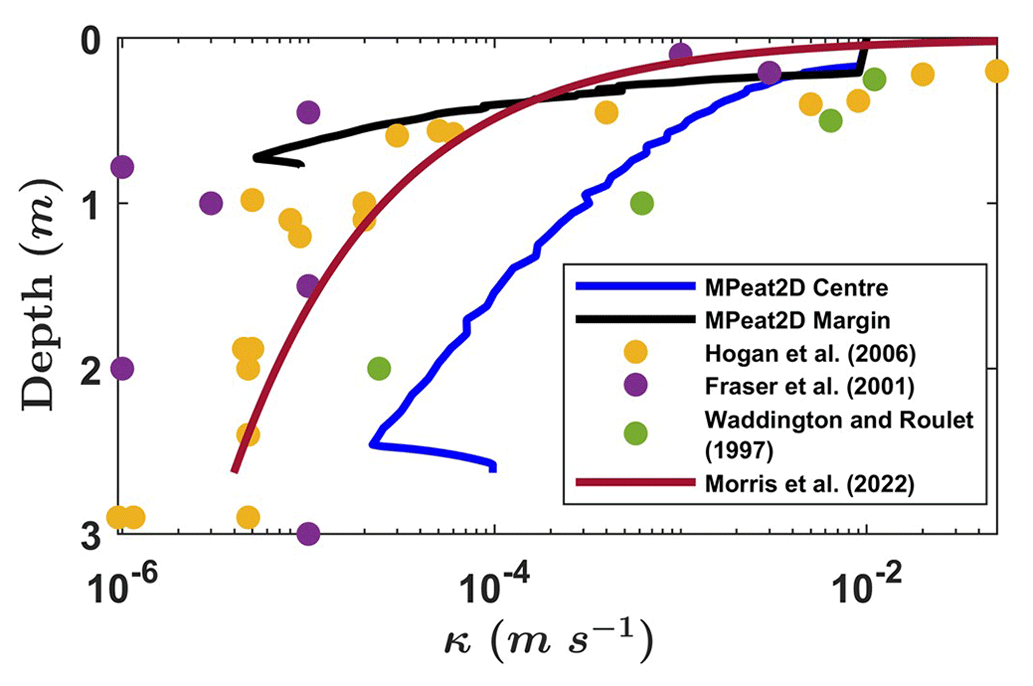
Figure 14 The comparison between hydraulic conductivity obtained from MPeat2D with field observations from Hogan et al. (2006), Fraser et al. (2001), and Waddington and Roulet (1997) and with another hydraulic conductivity model developed by Morris et al. (2022).

The peat thickness and carbon accumulation rate from MPeat2D, which are calculated based on the total amount of peat and carbon with the total simulation time, appear to be realistic. MPeat2D produces an average growth rate of about 0.52 mm yr⁻¹, which leads to a height of 2.61 m after 5000 years (Fig. 10b). Aaby and Tauber (1975) analysed the correlation between the rate of peat accumulation and the degree of humification that produced the growth rate of raised peatland in the range of 0.16–0.80 mm yr⁻¹ with an average value of 0.44 mm yr⁻¹. Aaby and Tauber (1975) suggested that the relationship between the degree of humification and the growth rate is affected significantly by mechanical compaction. A more decomposed peat experiences a higher compaction effect due to the reduction in Young's modulus and strength (Mahdiyasa et al., 2023, 2022), which results in a lower peat thickness. Furthermore, the average value of the net rate of carbon accumulation obtained from MPeat2D is about 0.0183 $\mathrm{kg}\mathrm{C}{\mathrm{m}}^{-\mathrm{2}}{\mathrm{yr}}^{-\mathrm{1}}$ (Fig. 10c), which is in agreement with the reported measurements of northern peatlands during the Holocene, with an average value around 0.0186 $\mathrm{kg}\mathrm{C}{\mathrm{m}}^{-\mathrm{2}}{\mathrm{yr}}^{-\mathrm{1}}$ (Yu et al., 2010, 2009).

5.2 Comparison with the other two-dimensional peatland development model

We emphasise the critical function of mechanical–ecohydrological feedback to simulate peatland development in 2D by comparing MPeat2D with the other ecohydrological model DigiBog (Baird et al., 2012; Morris et al., 2012). Using the same assumption of the flat and impermeable substrate with a constant climate, both models produce dome shapes of the peatland over 5000 years (Fig. 11a). However, the inclusion of mechanical–ecohydrological feedback on MPeat2D provides a plausible profile of bulk density (Fig. 5b) and active porosity (Fig. 5d) that are assumed to be a constant by DigiBog. Consequently, in the early stage of development, the value of bulk density from MPeat2D is lower than DigiBog, producing a more rapid increase in peat thickness and a faster appearance of the unsaturated zone (Fig. 11b). As peatland grows, the changes in peat physical properties and the discrepancy in the hydraulic gradient obtained from MPeat2D lead to the spatial variation in the water table depth, which is in line with the field observations (Reeve et al., 2006; Lewis et al., 2012; Kværner and Snilsberg, 2011; Regan et al., 2019). Furthermore, the water table depth decreases as the peatland develops in MPeat2D, resulting in wetter conditions for the peatland due to a more significant effect of compaction that supports the water accumulation. Contrastingly, DigiBog produces a relatively uniform hydraulic gradient, leading to the constant water table depth between the centre and the margin during the simulation period. This condition limits the capabilities of DigiBog to analyse the lateral variation in peat production, decomposition, and PFT proportion because these peatland characteristics depend on the water table depth (Clymo, 1984; Belyea and Clymo, 2001; Moore et al., 2002; Kokkonen et al., 2019; Laine et al., 2021).

The inclusion of mechanical–ecohydrological feedback also produces a more plausible shape of the peatland in 2D. Although MPeat2D suffers from the appearance of a cliff at the margin as DigiBog (Fig. 11a), the influence of mechanical compaction on MPeat2D results in a lower cliff height than DigiBog. The peat cliff at the margin does not appear in the natural condition, except due to extraction or erosion (Tuukkanen et al., 2017; Tarvainen et al., 2022). Furthermore, the continuum concept (Irgens, 2008; Jog, 2015) employed by MPeat2D produces the continuous deformation of the peat pore space, resulting in the smoother profile of peatland shape, especially near the margin, than DigiBog that uses linked vertical column (Fig. 11a). The comparison of the predicted peatland shape from MPeat2D with the groundwater mound hypothesis (GMH) (Ingram, 1982) indicates that MPeat2D produces a lower hydraulic gradient at the margin compared to the hemi-ellipse shape from GMH. The hemi-ellipse shape is obtained by assuming constant hydraulic conductivity throughout the peatland area, which is not true because the field observations from Baird et al. (2008) and Lewis et al. (2012) showed that the hydraulic conductivity changes in the vertical and horizontal directions. Armstrong (1995) modified GMH by proposing non-uniform hydraulic conductivity that exponentially decreases with depth, resulting in a lower hydraulic gradient at the margin and a more significant thickness at the centre, which agrees with MPeat2D. Furthermore, the work of Cobb et al. (2024) on the shape of peatlands demonstrates that appropriate comparative profiles are not hemi-elliptical as the marginal gradients are much more linear. The only profile that approximates a hemi-ellipse is for tropical peatland. The more linear gradient towards the margins rather than a marked curvature is the result obtained by MPeat2D. One of the most critical characteristics of the hemi-elliptical shape is the increasing curvature of the gradient toward the margin. However, MPeat2D predicts the peatland shape under idealised conditions, including fixed horizontal domain, flat substrates, and constant river elevation at the edges. Removing these assumptions might produce different peatland shapes and enhance the application of MPeat2D.

The comparison of MPeat2D with the more recent DigiBog versions (e.g. Young et al., 2017, 2019, 2021) shows some differences in the model formulation and parameterisation. MPeat2D allows the bulk density, active porosity, and hydraulic conductivity to change as a consequence of internal feedback mechanisms through the deformation of the peat pore space. Contrastingly, the more recent DigiBog versions employ empirical relationships to model the variation in hydraulic conductivity and assume constant values of bulk density and active porosity during the development process of the peatland. MPeat2D captures the spatial variability in the plant functional type composition, which affects the loading and rate of peat production, while the more recent DigiBog version ignores this factor in the model formulation. However, the more recent DigiBog version includes the parameters of mineral soil and water ponding thickness, which are omitted by the MPeat2D.

5.3 Limitations and future development

MPeat2D assumes a uniform distribution of peat throughout the fixed horizontal domain in the initial stages of development, which results in the omission of the lateral expansion process as the peatland grows. The lateral expansion is crucial to model the paludification that influences peatland behaviour because the transition from forest to peatland involves changes in vegetation, nutrient availability, and peat physical properties (Charman, 2002; Anderson et al., 2003; Rydin and Jeglum, 2006). Peatland lateral expansion requires an evolving domain that results in moving boundary problems (Tezduyar, 2001; Gawlik and Lew, 2015). Simplifying assumptions may be necessary to involve the moving boundary conditions into MPeat2D, including providing the rate of lateral expansion that determines the boundary motion and the changing domain. Moreover, to improve the numerical stability of the model, a smaller grid size might be required, particularly around the boundaries, due to significant differences in the internal stresses.

The assumption of a flat substrate employed by MPeat2D could be improved by introducing a more general landscape condition consisting of upland, sloping area, and lowland based on the theoretical landscape model proposed by Winter (2001). The landscape variations, together with the feedback from mechanical, ecological, and hydrological processes, affect the stresses on the peat body that control the occurrence of failure conditions on the peatland. The peatland failure involving mass movement (Dykes and Selkirk-Bell, 2010; Dykes, 2022, 2008) influences the estimation of carbon accumulation on the peatland because it might result in the formation of water channels that facilitate the drainage and oxidation processes (Warburton et al., 2003; Evans and Warburton, 2007). Potentially, this phenomenon could determine the maximum limit to peatland carbon accumulation in a landscape (Large et al., 2021).

The entrapped gas bubbles that are neglected by the current version of MPeat2D might have a significant influence on the peatland mechanics and behaviour. The presence of gas bubbles influences hydraulic conductivity (Baird and Waldron, 2003; Beckwith and Baird, 2001; Reynolds et al., 1992) and pore pressure (Kellner et al., 2004), which results in variations in effective stress. Consequently, the mechanical deformation of peat pore space, including the shrinking or swelling, is also affected by the presence of gas bubbles. The simulation from Reeve et al. (2013) suggested that a higher gas content results in a more significant peatland surface deformation. We could expand the poroelasticity formulation in the MPeat2D to accommodate the gas bubbles by introducing another fluid below the water table, for example, a water and gas mixture (Kurzeja and Steeb, 2022). This modification requires generalisation in Biot's theory of consolidation to model multiphase fluid saturation.

The current version of MPeat2D is focused on modelling raised ombrotrophic peatland which grows in temperate climates. However, it should be possible to develop MPeat2D to model the other peatland types, for example, the tropical peatland. Modifications of some processes are required before applying MPeat2D to analyse the peatland in tropical areas, including the variation in the rate of peat production, peat physical property characteristics, and loading behaviour. MPeat2D uses the empirical relationship between peat production and water table depth which is formulated based on the data from Ellergower Moss, Scotland (Belyea and Clymo, 2001). The rate of peat production in the tropical peatland is different from the northern temperate peatland due to the variations in the vegetation composition and climate. The hydraulic conductivity of tropical peatlands is very high compared to the northern temperate peatland (Baird et al., 2017), which might lead to different hydrological processes. Moreover, the loading from trees and the influence of roots for maintaining mechanical stability are significant processes in tropical peatlands which require an additional formulation in the MPeat2D. For example, the weight of trees with a root system could be modelled through the data of above-ground and below-ground biomass. In this case, the loading is applied not only at the top surface but also at the specific depth of the peatland, depending on the root characteristics.

Finally, the development of MPeat2D into a three-dimensional (3D) model provides a more comprehensive analysis of the peatland carbon accumulation process and phenomena that require explicit spatial interactions in 3D. The comparison between MPeat2D and MPeat indicates the crucial function of adding a second dimension to estimate peatland carbon accumulation. MPeat2D produces greater cumulative carbon, particularly under a non-constant climate, due to the lateral variability in the water table depth and peat physical properties incorporated by the 2D model. Based on this preliminary result, it might be possible that a 3D model of peatland development might result in a more significant carbon accumulation than the 1D or 2D models because of the more complex feedback mechanisms involved by a higher-dimensional model. The 3D model is also required to understand the patterning phenomena on the peatland surface, which is highly directional and affected by spatial characteristics. The analysis of surface patterning is typically developed based on ecohydrological feedback, which encompasses the interactions between water table position, vegetation communities, nutrient availability, and peat hydraulic properties (Eppinga et al., 2009, 2008; Morris et al., 2013; Béguin et al., 2019). However, as a porous medium with relatively low shear and tensile strength (Long, 2005; Boylan et al., 2008; O'Kelly, 2017; Dykes, 2008), the mechanical instability also determines the process of surface patterning on the peatland. The simulation from Briggs et al. (2007) indicates that the peatland surface might experience wrinkles due to the changing pattern between tensile and compressive stresses. Peatland surface patterns could appear as a consequence of the tensile or compressive failure condition (Dykes, 2008), which dominantly occurs under a low slope angle (Dykes and Selkirk-Bell, 2010). Therefore, a fully coupled mechanical, ecological, and hydrological model of peatland growth in three dimensions might be suitable for analysing the appearance and impact of surface patterning on the peatland water flow and carbon balance.

6 Conclusion

MPeat2D is a two-dimensional peatland growth model that incorporates mechanical–ecohydrological feedback and the influence of spatial variability on peatland behaviour. This model is developed based on the poroelasticity and continuum concept, resulting in the plausible outputs of peat physical properties, water table position, and vegetation composition. MPeat2D produces a higher bulk density and lower active porosity and hydraulic conductivity at the margin compared to the centre due to the different effects of compaction, which are in accord with field observations. Furthermore, lateral variability in the water table depth because of the changes in the hydraulic gradient leads to different vegetation compositions between the margin and the centre. The comparison between MPeat2D and the other peatland growth models, MPeat and DigiBog, indicates the critical function of mechanical, ecological, and hydrological processes together with the feedback from spatial heterogeneity on the peatland shape, carbon stock, and resilience.