Impact of noise on landscapes and metrics generated with stream power models

The Stream Power Model (SPM) has become a cornerstone of quantitative geomorphology, widely used to predict landscape evolution including the generation, moderation, and lowering of Earth's topography, sedimentary flux and biogeochemical processes. It is well known that landscape geometries predicted by the SPM can be strongly influenced by noise. However, its impact on the uncertainties or probabilities of, for instance, drainage planform geometries and widely used metrics is poorly understood. Noise can be incorporated into SPM simulations in a variety of ways. For instance, random, low amplitude, topographic anomalies are often inserted into starting conditions to enhance the realism of calculated drainage networks. Spatio-temporal or quenched (frozen) noise also influence the trajectories of evolving landscapes. Our goal with this paper is to establish how noise impacts the probabilities of landscape geometries and the reliability of tectonic and erosional information recovered from them. A series of landscape evolution models are run in which different arrangements, distributions, and implementations of noise are added to models evolving under the same tectonic and erosional forcings to an equilibrium state. We quantify uncertainties that arise from incorporating different arrangements of typical (uniform; white) and naturalistic initial, quenched and spatio-temporal noise. We focus on three conclusions. First, tectonic rates and values of erosional-geometric parameters (e.g., concavity and steepness indices, Hack exponents) recovered via metrics-based approaches (e.g., slope-area, χ, length-area) are uncertain in the presence of noisy initial conditions. Recovered values from individual landscapes generated with the same distribution but different specific arrangement of noise are at least as uncertain as ranges attributed to, for instance, changes in aridity. In fact, even noise with amplitudes that are <1 % of cumulative uplift can cause tectonic rates to no longer be recoverable to within a factor of two of true values. These results emphasise the sensitivity of metrics that rely on calculating derivatives (e.g., slope-area, χ) to noise. Secondly, whilst noise can make landscape geometries highly uncertain (different in different simulations), the distributions of their geomorphic properties (e.g., hypsometries, channel length-area relationships, Hack exponents) appear to have well defined statistical properties (e.g., expected values and variance). Finally, we suggest that a useful way to assess the impact of noise on SPM predictions is to generate ensembles of hundreds to thousands of models in which different arrangements of the chosen distribution of noise are inserted. Doing so can provide means to quantify uncertainty in predicted geometries and derived metrics, which can be substantial.

1 Introduction

It is well established that processes acting to shape Earth's topography leave behind some record of their history. Therefore interrogation of surface topography can, we hope, yield insight into how these processes operate and intertwine. Various observational and theoretical approaches exist to make such interrogations (e.g., Anderson and Anderson, 2010). One family of approaches makes use of partial differential equations (PDEs), often solved numerically, to predict evolution of topography in space and time. The Stream Power Model (SPM) is perhaps the most widely used (see e.g., Howard, 1994; Rosenbloom and Anderson, 1994; Whipple and Tucker, 1999; Tucker and Hancock, 2010; Lague, 2014; Salles, 2016; Hobley et al., 2017, and references therein). A wide variety of metric-based, forward and inverse modelling studies utilise the SPM to derive information about uplift, erosion, climate and biogeochemical processes from real and synthetic landscapes (e.g., Howard, 1994; Whipple and Tucker, 1999; Baldwin et al., 2003; Zaprowski et al., 2005; Roberts and White, 2010; Roberts et al., 2012a; Ferrier et al., 2013; Croissant and Braun, 2014; Forte et al., 2016; Harel et al., 2016; Mitchell and Yanites, 2019; Campforts et al., 2020; Lipp et al., 2020, 2021; Salles et al., 2023; DeLisle and Yanites, 2024). However, one complication to this endeavour is the presence of noise, which we consider in two categories.

The first category of noise, obfuscating the recovery of tectonic information, we term as “scientific”. By this we refer to things which cannot be known, such as the many areas within a landscape that have unknown or poorly understood histories, where information necessary to recover tectonic information has been removed by erosion, for instance. This category also includes noise that can be attributed to measurement or observational uncertainties due to, for example, fluctuations or changes in landscape form that are too rapid or slow to be recorded directly (Lague, 2014; Ancey et al., 2015; Forte et al., 2016; Chen et al., 2022; Roberts and Wani, 2024).

The second category of noise we consider, and the focus of this paper, is computational. A usual strategy in landscape evolution models is for computational noise to be inserted as random elevations within a model starting condition to enable realistic drainage networks to form (see e.g., Willgoose et al., 1991; Tucker and Slingerland, 1994; Braun and Sambridge, 1997; Smith et al., 1997; Tucker et al., 2001; Coulthard et al., 2012; Goren et al., 2014, and references therein). Typically, initial topographic roughness is drawn from a random uniform distribution (i.e., white noise). Other types of noise have been incorporated into landscape simulations, such as those with normal distributions or generated using specific algorithms (e.g., Perlin noise; diamond square algorithm), though they are less common (Fournier et al., 1982; Perlin, 1985, 2002; Perron and Fagherazzi, 2012; Mudd et al., 2018; Etherington, 2022; Ruiz Sánchez-Oro et al., 2024). The choice of noise (e.g., its distribution) has important implications for landscape geometries, however the often assumed white noise is not necessarily representative of observed topography or processes driving landscape evolution (see e.g., Ijjász-Vásquez et al., 1992; Perron and Fagherazzi, 2012; Kwang and Parker, 2019; Wapenhans et al., 2021). Whilst specific details of palaeotopography may not be knowable, spectral analysis of modern topography provides insight into the distributions of elevations that we might wish to replicate when deciding on the distributions of noise to be used within, for instance, model starting conditions (Perron et al., 2008; Audet, 2011; Roberts et al., 2019; Wapenhans et al., 2021). We note that alternative approaches to generate realistic channel planforms exist outside of adding random elevations. One option is to randomise flow directions (e.g., Salles, 2016; Salles and Hardiman, 2016). However given the extensiveness of adding noisy random elevations to encourage LEMs to channelise, we focus our attention of the consequences of doing so in this study.

The presence of noise within natural and modelled landscapes is known to complicate the recovery of geomorphic information. Roberts et al. (2012b) and Smith et al. (2022) showed how solutions recovered from channel slope-upstream drainage area data become unstable when noise is added to longitudinal profiles. Castelltort and Yamato (2013) highlight how the steepness of slopes present in noisy initial conditions added to LEMs can unsatisfactorily influence the geometry of resultant drainage basins. Wapenhans et al. (2021) demonstrate that adding white noise to longitudinal river profiles extracted from a landscape evolution model leads to changes in power spectra that increase their similarity to power spectra of observed rivers. Addition of quenched noise to landscape evolution models can have similar effects (Birnir et al., 2001; Wapenhans et al., 2021). Several studies have sought to recover erosional parameter values using SPMs by maximising the similarity of predicted topography to observed landscapes (Croissant and Braun, 2014; Barnhart et al., 2020c). It is likely that the presence of noise contributes to a range of acceptable values being recovered (Willgoose et al., 2003). Inverse approaches such as these require the construction of a misfit function to quantitatively compare observations to model predictions. However, inserted noise is known to impact drainage planforms, which can persist throughout a model run time (Ijjász-Vásquez et al., 1992; Willgoose et al., 2003; Perron and Fagherazzi, 2012; Hancock et al., 2016; Kwang and Parker, 2019). An important challenge is to generate misfit functions that are insensitive to noise so that insight into the processes that drive topographic change such as uplift can be recovered with accurate assessment of uncertainties (Willgoose et al., 2003; Morris et al., 2023).

In this study we seek to establish an understanding of the role of noise within landscape evolution models and its consequences for a variety of commonly used geomorphic metrics and tools. We design four scenarios to assess how different distributions of noise and the way in which they are inserted into the SPM impact the variance of basic geometric properties: elevations, planforms, hypsometry, spectral content, and fluvial information: longitudinal profiles, slope-area relationships, χ-elevation profiles, length-area relationships. We also assess the variance of erosional parameter values and uplift rates calculated from widely used metrics (slope-area, χ), quantifying the impact of noise on the reliability of information recovered. Given the ubiquity of assumed steady state in studies making use of the SPM, we focus on assessing the impact of noise on landscapes that are demonstrably at, or very close to, topographic steady state, which we define here as (practically) no elevation change in any grid cell between successive model time steps and explain further in Sect. 2.4 (Willett and Brandon, 2002).

2 Methodology

In this section we first describe how synthetic landscapes and noisy functions are generated. We then describe how steady state conditions are identified, and the modelling strategy used to assess the impact of noise on geomorphic metrics.

2.1 Generating synthetic landscapes

In this study, landscape evolution is modelled using a widely accepted grid-based framework in which we implement a partial differential equation (PDE) governing the rate of change, and evolution, of elevations. We make use of gridding, flow routing, and numerical PDE solver libraries that are part of the Landlab toolkit to generate synthetic landscapes (Hobley et al., 2017; Barnhart et al., 2020a; Hutton et al., 2020). The erosional model and uplift rates are defined, and noise is added, such that

$$\begin{array}{}\text{(1)}& {\displaystyle \frac{\partial z}{\partial t}}=-K{A}^m\mathrm{\nabla }{z}^n+\mathit{\kappa }{\mathrm{\nabla }}^{\mathrm{2}}z+U+\mathit{\eta },\end{array}$$

where z is elevation, t is time, and K, m, n, and κ are erosional constants. The erosional processes (first two terms on RHS of Eq. 1) can be regarded as being a simple version of the (advective) stream power model, and erosion that, phenomenologically at least, mimics diffusion, for instance “transport-limited” or hill-slope processes (see e.g., Howard, 1994; Rosenbloom and Anderson, 1994). For simplicity – we seek to avoid the complexities that arise when shocks are expected or thresholds are incorporated – and to aid assessment of the impact of noise, we implement a linear version of the stream power model, i.e., the slope exponent n=1 (we include the n notation for completeness; see e.g., Pritchard et al., 2009; Lague, 2014; Roberts and Wani, 2024). Upstream drainage area, $A=A(x,y,t)$, uplift rate, $U=U(x,y,t)$, and noise, $\mathit{\eta }=\mathit{\eta }(x,y,t)$ can vary as a function of space, (x,y), and time.

Each synthetic landscape in this study is generated by the following steps (Fig. 1). First, a uniform Cartesian (raster) grid with dimensions of 100 × 100 km and cell size of 1 × 1 km is generated. Elevations at the boundaries of the domain are fixed at zero (i.e., Dirichlet conditions). Each “east”, “west”, “south” or “north” boundary is individually set to be open/active (i.e., flux across it is permitted) or closed/inactive (i.e., flux is forbidden; see Hobley et al., 2017 for details). An initial (noisy) topography is then added to the grid. It is the choice of this initial topography, subsequent additive noise, and their consequences on resultant landscape evolution and associated metrics that are the foci of this paper. Topographic depressions are then filled to permit continuous flowlines and minimise the chance of internally draining regions forming (Barnes et al., 2014). Erosional parameters m=0.5 and $K={\mathrm{10}}^{-\mathrm{3}}$ kyr⁻¹. Erosional “diffusivity” κ = 100 m² kyr⁻¹. Diffusion is calculated using the explicit finite-volume method within the Landlab model component LinearDiffuser, with deposition turned off. The advection component of erosion is calculated using the FastScape erosion scheme, and flow routing is performed with the “D8” algorithm (O'Callaghan and Mark, 1984; Braun and Willett, 2013). In other words, the basic modelling framework is purposefully simple and designed to honour the assumptions that underpin the calculation of many geomorphic metrics. Each synthetic landscape is evolved forwards in time for 100 Myr, with uplift, flow-routing, erosion, and diffusion taking place at each model time step. We use a model time step, Δt=10 kyr, which satisfies the Courant-Friedrich-Lewy (CFL) condition and is sufficiently large that computational runtime is reasonable. This value provides numerical stability and demonstrable convergence.

2.1.1 Three categories of landscape configuration

We generate three categories of relatively simple synthetic landscapes designed to resemble widely studied natural and computational end-members: a “block” of topography uplifted at a constant rate, escarpment evolution, and evolution of a topographic swell/dome (see e.g., Beaumont et al., 1992; Kooi and Beaumont, 1994; Tucker and Slingerland, 1994; Braun and van der Beek, 2004; Pelletier, 2007; Anderson and Anderson, 2010; Roberts and White, 2010; Braun et al., 2013; Paul et al., 2014; Hobley et al., 2017; O’Malley et al., 2021; Gasparini et al., 2024). The first category has open boundary conditions along each edge of the model domain, for all other (core) grid cells uplift rate is constant, $U(x,y)=\mathrm{0.2}$ m kyr⁻¹. We henceforth refer to this category as producing “square” landscapes. The second category has open boundary conditions along the east and west edges of the model domain only; no flux is permitted along the north and south boundaries. Uplift is again as a “block” with U=0.2 m kyr⁻¹. This category produces “escarpment” landscapes. The third category has open boundaries and a Gaussian uplift function, decaying from the centre of the domain towards its edges with the form

$$\begin{array}{}\text{(2)}& U(x,y)=U_{max}\exp \left\{-\left[{\displaystyle \frac{(x-x_{\mathrm{0}}{)}^{\mathrm{2}}}{\mathrm{2}{\mathit{\sigma }}_x^{\mathrm{2}}}}+{\displaystyle \frac{(y-y_{\mathrm{0}}{)}^{\mathrm{2}}}{\mathrm{2}{\mathit{\sigma }}_y^{\mathrm{2}}}}\right]\right\},\end{array}$$

where U(x,y) is uplift rate, $x_{\mathrm{0}}=y_{\mathrm{0}}=\mathrm{50}$ km are the central coordinates of the dome, and ${\mathit{\sigma }}_x={\mathit{\sigma }}_y=\mathrm{20}$ km are the standard deviations (spreads) in the x and y directions. The function is scaled by maximum uplift rate, $U_{max}=\mathrm{0.2}$ m kyr⁻¹. This category produces “domal” landscapes. Examples of the “square”, “escarpment”, and “domal” landscape are shown in Fig. 1. We maintain this nomenclature throughout to describe the three categories of landscape configuration.

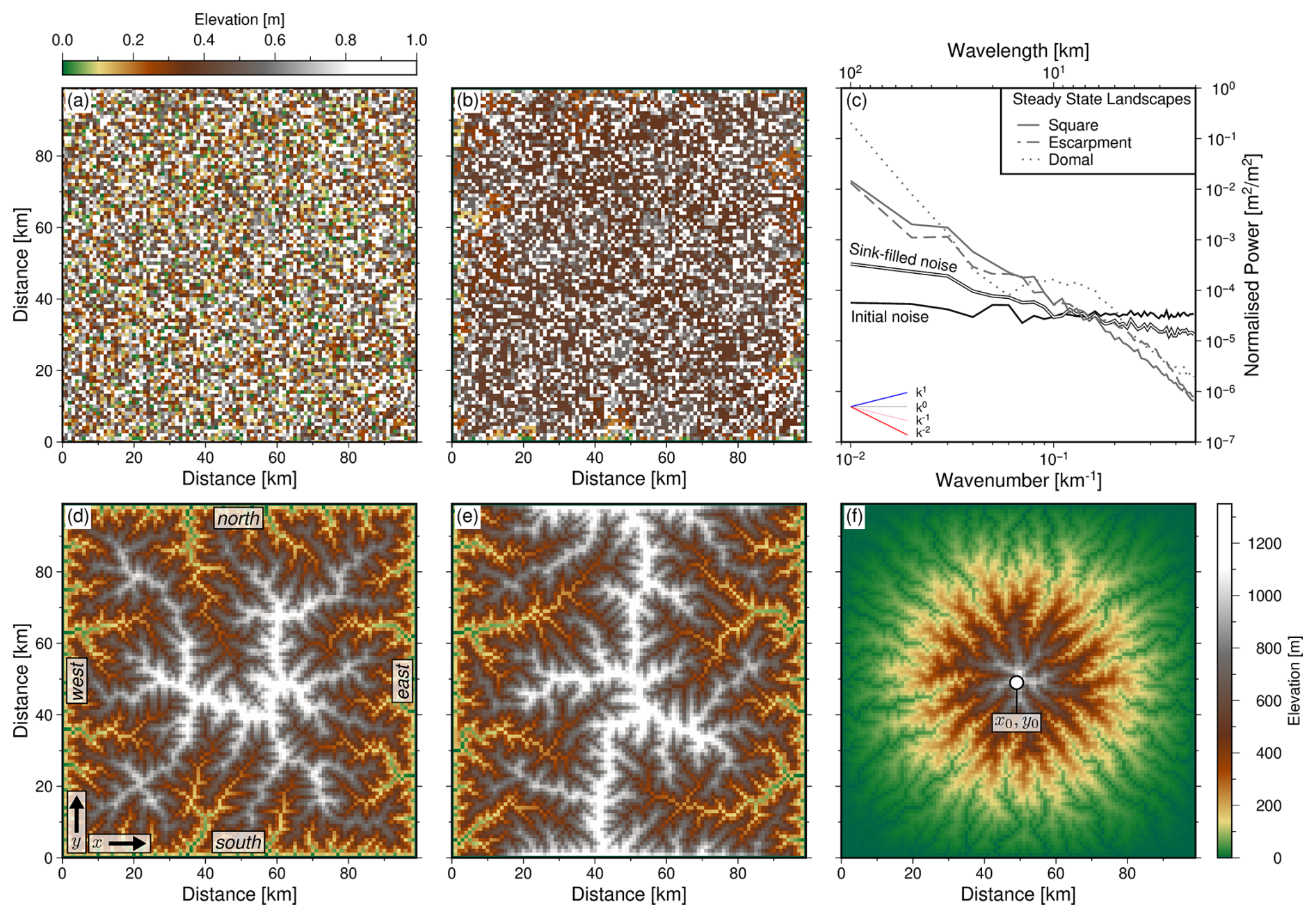
Figure 1 Introduction to geometries and power spectra of landscapes generated using the Stream Power model. (a) Initial white (“uniform”) noise; typically used when parametrising landscape evolution models to ensure realistic looking drainage planforms emerge. (b) The white noise function shown in panel (a) once sinks have been filled; a standard step that seeks to ensure drainage networks are continuous. (c) Normalised power spectrum – ϕ(k), where ϕ is radially averaged (in the frequency domain) spectral power, and k is wavenumber, i.e., spatial frequency – of initial (a) and sink-filled noise (b), and of the three steady state landscapes shown in panels (d)–(f). Normalisation is for visual purposes only. Note graticule showing power spectral slopes of theoretical blue (ϕ∝k), white (ϕ∝k⁰), pink (ϕ∝k¹) and red (ϕ∝k²) noise. (d–f) Steady state landscapes generated with uplift rates that are constant in space and time, unless otherwise indicated (see body text for details). (d) “Square” landscape generated with fixed, open, boundaries. (e) “Escarpment” landscape with closed north and south boundaries. (f) “Domal” landscape generated with uplift rate modulated by a (spatial) Gaussian function (see Eq. 2).

2.2 Generating noisy functions and their verification

2.2.1 Introduction to noise in landscape simulators

In this section we describe how different distributions of noise can be produced and inserted into landscape evolution models. The resultant functions are used to define starting conditions and the additive noise inserted into the scenarios examined. We then demonstrate how the spectral content and characteristics, e.g., colours of noise, of such functions and of evolved landscapes can be assessed.

We focus on examining the impact of “end-members” – red, white and blue noise – for the following reasons. First, topography and many other natural phenomena (e.g., mantle convective support of Earth's surface, potential fields) tend to have red noise characteristics (see e.g., Bell, 1975; Rapp, 1989; Pelletier, 1999; Birnir et al., 2001; Turcotte, 2007; Singh et al., 2011; Valentine and Davies, 2020; Holdt et al., 2022, and references therein). For a landscape to have red noise characteristics it would have amplitudes of elevation that are inversely proportional to spatial frequencies, k (i.e., wavenumber), where $k=\mathrm{1}/\mathit{\lambda }$, λ is wavelength. Wavelength can be thought of as broadly synonymous with scale. In other words, as horizontal scales increase, so do vertical scales; wide features have big amplitudes, and narrow features have small amplitudes. Landscapes with red noise characteristics have spectral power, ϕ(k) proportional to k⁻², where ϕ=Z² with Z=Z(k) being elevations in the frequency domain. We discuss how such signals can be identified in the following section. In contrast, white noise (amplitudes are scale-invariant; ϕ∝k⁰), which appears to characterise some long-timescale atmospheric temperature variations and fossil records, for instance, is often assumed to be appropriate for parametrising landscape evolution models (see e.g., Ijjász-Vásquez et al., 1993; Howard, 1994; Smith et al., 1997; Kirchner and Weil, 1998; Pelletier, 1998; Yacobucci, 2005; Castelltort and Yamato, 2013; Adams et al., 2015; Gray et al., 2017; Lyons et al., 2020; Shen et al., 2021; Cullen et al., 2022). Blue noise, which appears to be a property of (at least some) systems that exhibit shockwave behaviour (e.g., perhaps at small scales in fluvial landscapes; Wapenhans et al., 2021; Wang et al., 2022; Roberts and Wani, 2024) would indicate that landscapes have vertical amplitudes proportional to wavenumbers, i.e., narrow features have big amplitudes, wide features have small amplitudes (ϕ∝k).

2.2.2 Generating white, red and blue noise

In order to generate a two-dimensional function, z(x,y), i.e., map of elevations, with a specific distribution (colour) of noise we first create a random uniform (white noise) function of size N_x×N_y, where N_x and N_y are equal to the number of cells in the x and y directions. Amplitudes are set to $\mathrm{0}\le z\le \mathrm{1}$ m. Such functions are straightforwardly generated using a variety of random number generators, such as Python's numpy.random.uniform, which we make use of. Generating white noise in this way is standard procedure in most simulations of two-dimensional landscape evolution (see e.g., Braun and Sambridge, 1997; Tucker et al., 2001; Goren et al., 2014; Gray et al., 2017; Lyons et al., 2020; Morris et al., 2023). Many white noise functions with different specific arrangements of elevations can be generated rapidly by re-running such algorithms with different “seed” numbers. Seed numbers are sometimes set “under-the-hood” using, for instance, computer clock time (see e.g., Press et al., 1992 for extended discussion of random number generation). In contrast, we define (and record) a unique seed number for each model, ensuring reproducibility.

Maps of elevation (e.g., white noise) in the spatial domain can be converted into the frequency domain using a two-dimensional discrete Fourier transform, such that

$$\begin{array}{}\text{(3)}& Z(k_x,k_y)=\sum _{j=\mathrm{0}}^{N_x-\mathrm{1}}\sum _{k=\mathrm{0}}^{N_y-\mathrm{1}}z(x,y)e^{-\mathrm{2}\mathit{\pi }i\left(k_x/N_x+k_y/N_y\right)},\end{array}$$

where k_x and k_y are the wavenumbers in the x and y directions, $i=\sqrt{-\mathrm{1}}$, j and k are index positions in the two-dimensional z(x,y) array (Cooley and Tukey, 1965; Press et al., 1992; Perron et al., 2008).

We use the wavenumber content of white noise functions, Z_w(k_x,k_y), to generate other functions that have different distributions (colours of noise), Z_η(k_x,y_y), in four steps. First, Z_w(k_x, k_y) is rearranged by shifting the zero-wavenumber component to the centre of the array. Second, the array is multiplied by the square root of the radial wavenumber, $f=f(k_x,k_y)$, raised to the power p,

$$\begin{array}{}\text{(4)}& Z_{\mathit{\eta }}(k_x,k_y)=Z_{\mathrm{w}}(k_x,k_y)\sqrt{{\left(f/f^{*}\right)}^p},\end{array}$$

where $f^{*}=\mathrm{1}$ km⁻¹ ensures dimensionality. The radial wavenumber, f, is given by

$$\begin{array}{}\text{(5)}& f(k_x,k_y)=\sqrt{(k_x-N_x/\mathrm{2}{)}^{\mathrm{2}}+(k_y-N_y/\mathrm{2}{)}^{\mathrm{2}}}.\end{array}$$

The exponent p controls how rapidly elevations change in the wavenumber domain. When p<0 longer wavelength signals have greatest amplitudes. The opposite is true when p>0. We generate red noise, Z_r, using $p=-\mathrm{2}$ , and blue noise, Z_b, with p=1. White noise maps have p=0. Third, the Z_η (Z_r or Z_b) array is converted from the frequency domain into the spatial domain by, first, reversing the shifting of zero-wavenumber components, and then calculating the inverse 2D discrete Fourier transform of the real components of Z_η(k_x,k_y).

Finally, we normalise the resultant function z_η(x,y) to ensure that elevations are between 0 and 1 m. Normalisation is achieved by adding the minimum elevation to the entire array, and dividing through by the new maximum elevation:

$$\begin{array}{}\text{(6)}& z_{\mathit{\eta }}(x,y)={\displaystyle \frac{\left|z_{\mathit{\eta }}\right(x,y)+z_{\mathit{\eta }}^{min}|}{z_{\mathit{\eta }}^{max}}}.\end{array}$$

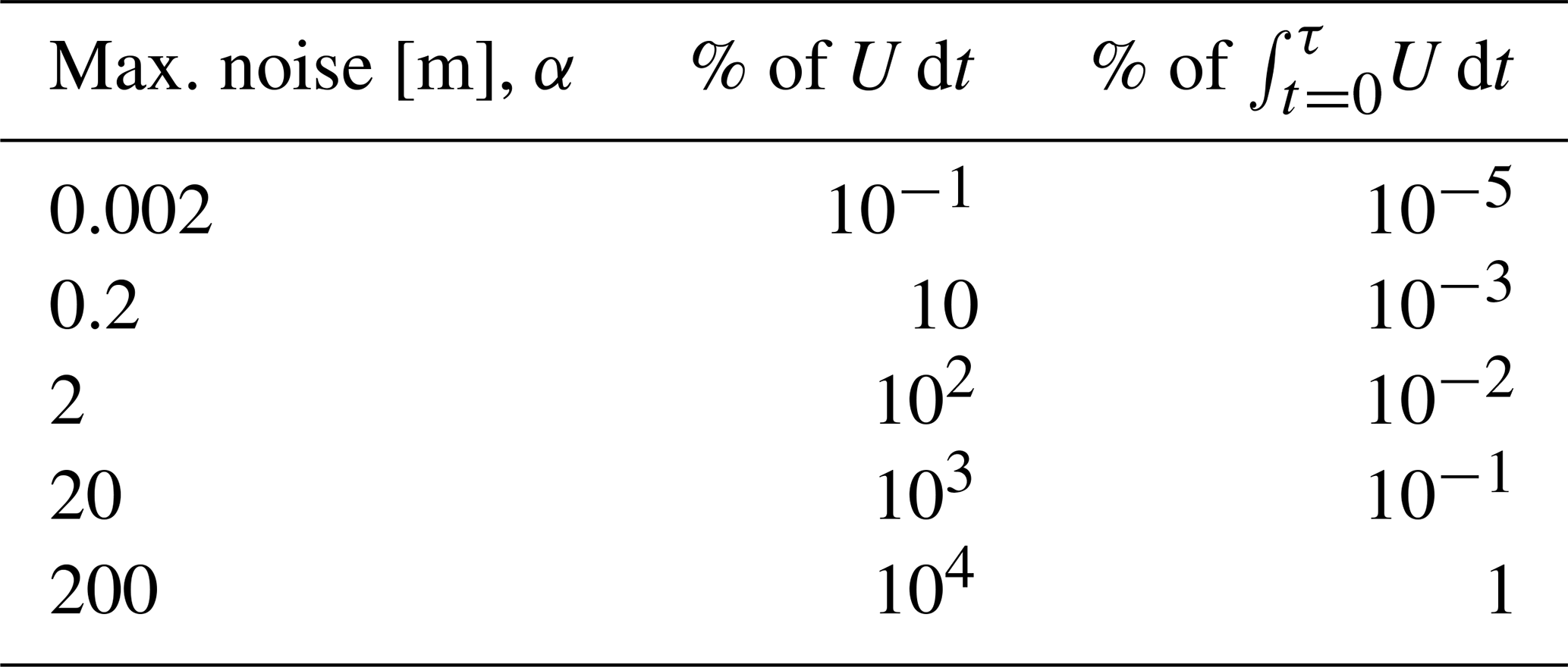
These steps are repeated multiple times to generate M functions with red, blue or white noise characteristics (Fig. 2). To test the impact of different amplitudes of noise, z_η(x,y) was scaled by a factor α (see Table 1). Histograms of elevations for these noisy functions are shown in Fig. S1 in the Supplement.

Table 1 Maximum amplitude of noise added to initial conditions, or each time step as percentage of uplift rate, U=0.2 m kyr⁻¹, or cumulative uplift after τ=100 Myr.

2.2.3 Power spectra

The noise characteristics of these functions are verified by first inserting them into Eq. (3) and then calculating their power spectra,

$$\begin{array}{}\text{(7)}& \mathit{\varphi }(k_x,k_y)={\displaystyle \frac{\mathrm{1}}{N_x^{\mathrm{2}}{N}_y^{\mathrm{2}}}}\left|Z_{\mathit{\eta }}\right(k_x,k_y){|}^{\mathrm{2}}.\end{array}$$

Since two-dimensional power spectra, ϕ(k_x,k_y), can be challenging to interpret they are usually visualised in one dimension (i.e., ϕ(k); see e.g., McKenzie and Bowin, 1976; McKenzie and Fairhead, 1997; Perron et al., 2008; Watts and Moore, 2017). There are two quite widely used methods. The first approach calculates mean power between specific radial frequencies (from the zero-shifted power spectrum) by averaging within annuli, in our case we average within sequential annuli of width δf=1 km⁻¹ (see e.g., McKenzie and Bowin, 1976). Figure 2 shows the power spectra of 100 red, white and blue noise functions generated in this way. It demonstrates that these functions have respective power spectra that on average are proportional to k⁻², k⁰ and k, as expected.

The second approach simply collapses the two-dimensional spectra into one dimension, such that each “pixel” ϕ(k_x,k_y) can be plotted as ϕ(k) (see e.g., Perron et al., 2008; Watts and Moore, 2017). In practice, if appropriate values of δf are chosen, the one dimensional spectra from both approaches are very similar. We present collapsed power spectra of elevations, following transformation $z(x,y)\to Z(k_x,k_y)\to \mathit{\varphi }\left(k\right)=Z^{\mathrm{2}}\left(k\right)$, in later figures because they demonstrate the solutions to Eq. (7) directly. Also shown in these figures is mean power,

$$\begin{array}{}\text{(8)}& \stackrel{\mathrm{‾}}{\mathit{\varphi }\left(k\right)}=\langle \mathit{\varphi }\left(k\right)\rangle ,\end{array}$$

where the angle brackets denote the average value for a wavenumber band centred on wavenumber k. We perform the averaging within logarithmically equally spaced bands. The Code and Data Availability statements explain where Python scripts to generate and verify noise maps can be found.

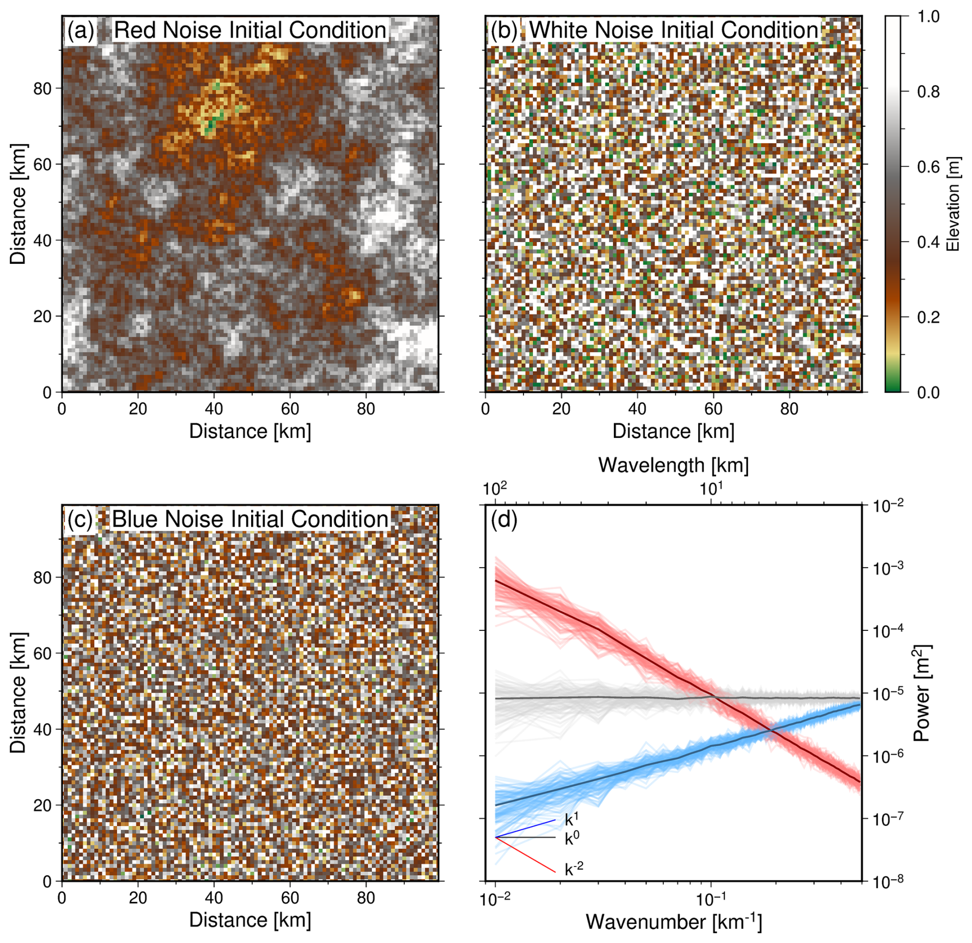
Figure 2 Noise functions (maps) used to generate initial conditions for landscape models. (a–c) Examples of functions with red, white and blue noise characteristics. (d) Thin red lines = radially averaged (in the frequency domain) power spectra, ϕ(k), of the 100 red noise functions used in this study (see body text for details). Thin grey and blue lines = respective power spectra of the 100 white and blue noise functions used in this study. Thick lines = average values for each suite of coloured functions. Note graticule showing theoretical spectral slopes for red ($\mathit{\varphi }\propto k^{-\mathrm{2}}$, where k = wavenumber), white (ϕ∝k⁰), and blue (ϕ∝k) noise.

2.3 Experimentation strategy

Figures 3 and 4 summarise our approach to experimentation. Our goal with this strategy is to establish the impact of noise on landscape evolution in a series of increasingly complex, and perhaps more realistic, scenarios.

In scenario A, we examine the consequences of a widely used approach – insertion of noise only into the starting condition of a landscape evolution model (see e.g., Braun and Sambridge, 1997; Tucker et al., 2001; Braun and Willett, 2013; Goren et al., 2014; Barnhart et al., 2020a, b, c). We examine the impact of different distributions (i.e., red, white, blue) and amplitudes of noise. Each ensemble examined (e.g., white noise, “square” landscape; white noise, “escarpment” landscape; white noise, “domal” landscape; red noise “square” landscape, etc.) contains M=100 or M=1000 individual models. Within an ensemble, each model has the same boundary conditions, uplift function, erosional parameter values, and distribution of noise, but crucially they all have different specific arrangements of noisy elevations; different “seeds” were used to generate noise in each model. The resultant M landscape geometries were used to gain statistical insight into the impact of noise on landscape evolution, form and recovery of geomorphic metrics. Figure 4 summarises the ensembles tested (scenario A: ensembles 1–18).

In scenario B we test the impact of quenched (i.e., “frozen”) noise. For an individual model, a noisy function is added to its starting condition (as in scenario A), then the exact same arrangement of noisy elevations is inserted at every subsequent time step (Fig. 4: ensembles 19–21). A rationale for testing such a scenario arises from the work presented in Birnir et al. (2001) and Wapenhans et al. (2021), which demonstrate the need for landscape evolution models to incorporate additive noise to avoid artificial spectral reddening of landscapes, i.e., unrealistic reductions in topography at short wavelengths (small scales). Incorporating noise in this way is loosely related to modelling studies that seek to assess the impact of substrate on landscape evolution by changing erodibility (see e.g., Sklar and Dietrich, 2001; Haviv et al., 2010; Forte et al., 2016; Campforts et al., 2020).

Scenario C again includes noise added to the starting condition. However, in contrast with scenario B, different arrangements of the same underlying distribution (colour) of noise are added to each model at every time step. In other words, noise varies as a function of space and time. Arguably, this approach is more realistic than scenarios A and B, and probably more appropriate when specific arrangements of noise are likely to be unknown. Figure 4 (ensembles 22–24) summarises this experimentation.

The noise added throughout models within Scenarios B and C has amplitudes of 0–1 m. We choose to incorporate additive noise for two reasons. First, to maintain consistency with the amplitude of noise added to the starting condition, and second, to avoid cases in which regions of internal drainage may arise, thus potentially requiring additional (ad hoc) sink-filling steps. However we acknowledge that this may not necessarily represent noisy surface processes which act to alter topography. Instead, such processes may also reduce elevations. Whilst it is generally unclear what an appropriate mean elevation might be in order to represent these processes, we also perform an additional set of simulations in the style of Scenarios B and C with noise of −0.5 to 0.5 m amplitude (i.e. mean elevation = 0). Results for these tests are shown in Supplement Fig. S9 and S10.

Scenarios A–C have flow routing and erosion applied in their final time step, after noise has been inserted. Thus, inserted noise is eroded for 10 kyr (i.e., the length of the time step) before metrics are extracted. In actuality, noise could be inserted into a landscape at any time. Thus, we test scenario D in which noise is inserted into synthetic landscapes at the end of model run time. We take the steady state landscapes (at 100 Myr) generated by scenario A with 1 m of noise and insert noise with the same arrangement. The impact of inserting final noise with scaled maximum amplitudes of 2, 20 and 200 m is assessed (see Table 1). For clarity, metrics are extracted from the noisy landscapes using drainage planforms determined before final noise is added, i.e., no additional flow routing or sink filling is performed. This approach is a generalisation, to two dimensions, of that presented in Roberts et al. (2012b) and Smith et al. (2022), in which noise is added directly to the longitudinal profiles of rivers (Fig. 4: ensembles 25–27).

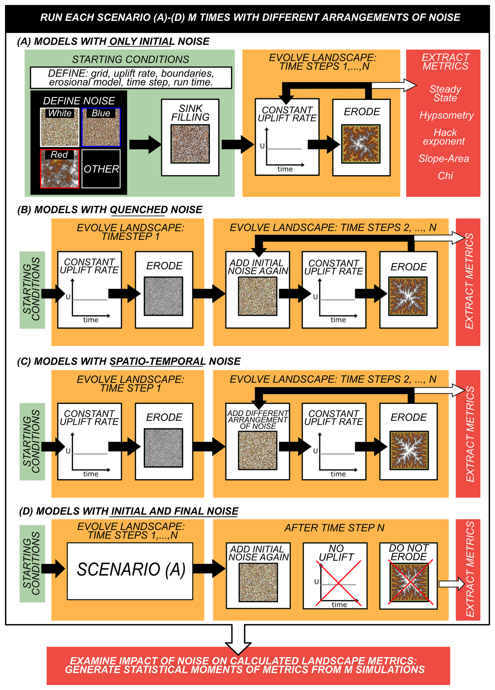
Figure 3 Schematic summarising the scenarios tested and approach to extracting metrics. In scenarios A–D forward models are initialised with starting conditions that include noise (white, blue or red in this study), they are then run for a specified number of time steps, evolving to steady state. Geomorphic metrics are extracted from steady state topography. Each scenario is run multiple (M) times using different arrangements of noise to generate statistical insights and assess stability of calculated metrics. The example demonstrated here is for the “square” landscape shown in Fig. 1d. Note that we also assess the impact of changing boundary conditions and uplift function, and scenarios when no noise is explicitly incorporated. Scenario A: Noise is only incorporated into the starting condition; the quintessential landscape evolution modelling strategy. Scenario B: Noise used in the starting condition is incorporated at each time step; testing the impact of quenched, “frozen”, noise. Scenario C: Different arrangements (but same distribution) of noise are incorporated at each time step. Scenario D: Uneroded noise is added to the landscape at the end of model run time.

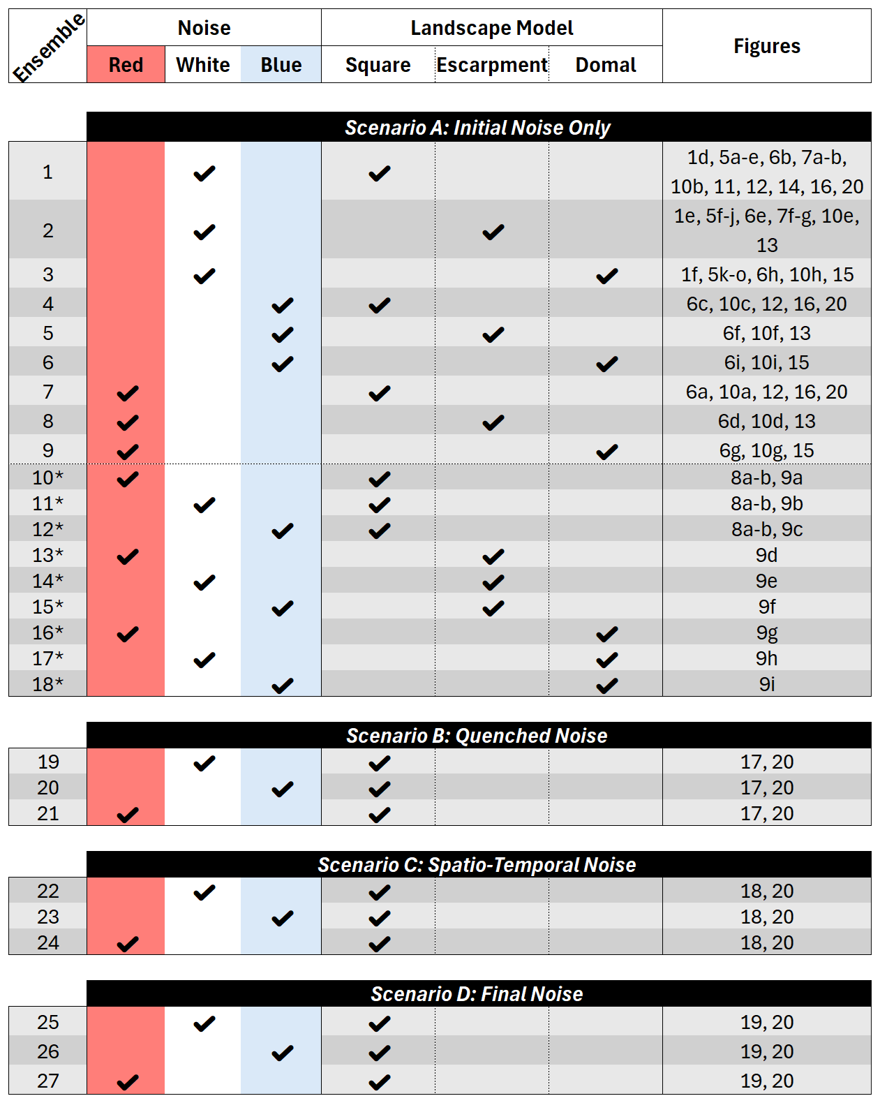
Figure 4 Guide to scenarios, ensembles and models in this study. Ensembles with asterisk (^*) contain M=1000 models, all others contain M=100 models.

2.4 Identifying steady state landscapes for experimentation

The assumption of topographic steady state remains widely used in quantitative studies of fluvial geomorphology (see e.g., Snyder et al., 2000; Istanbulluoglu and Bras, 2005; Attal et al., 2008; Perron and Fagherazzi, 2012; Theodoratos et al., 2018; Leonard and Whipple, 2021; Fisher et al., 2022; Clubb et al., 2023; Hoskins et al., 2023; Zhou et al., 2024). It underpins the use of a variety of geomorphic metrics used to generate quantitative estimates of erosional parameter values and uplift rates (see e.g., Wang et al., 2017). Thus, we run our models until they are demonstrably at, or get as close as reasonably possible to, steady state and then examine the impact of noise on calculated metrics. A variety of criteria can be used to define steady state topography in both natural (observed) and synthetic landscapes (see e.g., Willett and Brandon, 2002; Gasparini et al., 2024, and references therein). For clarity, in this paper steady state means $\partial z/\partial t=\mathrm{0}$, i.e., rate of change of elevation is invariant everywhere in the landscape.

As Gasparini et al. (2024) explain, demonstrating that a synthetic landscape is at topographic steady state is not necessarily trivial, we extend their approach here. A useful attribute of landscape evolution modelling is that it is straightforward to extract and visualise distributions of topographic change over consecutive time steps, which can be used to assess topographic (in)transience. Figure 5 shows three statistics used to assess topographic steady state. First, following Gasparini et al. (2024), we extract the maximum local change in elevation, Δz, across the entire model domain between consecutive time steps

$$\begin{array}{}\text{(9)}& \mathrm{\Delta }{z}_{\mathit{\alpha }}^t=max\left(\right|z_i^t-z_i^{t-\mathrm{\Delta }t}\left|\right),\end{array}$$

where i here indicates the index of all elevations ($i=\mathrm{1},\mathrm{\dots },N_x{N}_y$), and t is the index of time steps. Similarly, the change in mean elevation of the entire domain, from one time step to the next, is calculated,

$$\begin{array}{}\text{(10)}& \mathrm{\Delta }{z}_{\mathit{\beta }}^t=|\stackrel{\mathrm{‾}}{z^t}-\stackrel{\mathrm{‾}}{z^{t-\mathrm{\Delta }t}}|,\end{array}$$

where $\overline{z}$ is the mean elevation of a landscape. Change in maximum elevation between consecutive time step is also extracted,

$$\begin{array}{}\text{(11)}& \mathrm{\Delta }{z}_{\mathit{\gamma }}^t=|max(z^t)-max(z^{t-\mathrm{\Delta }t}\left)\right|.\end{array}$$

Examples of these statistics are shown in Fig. 5 for three landscapes generated with white noise only in their initial conditions. Figures S7 and S8 similarly show statistics for typical landscapes generated within scenarios B and C.

In addition to such statistical approaches, it is beneficial to examine how distributions of elevation change evolve as the synthetic landscapes mature. Consequently, Fig. 5 shows histograms of topographic change between successive time steps for all cells within the three example landscapes. The histograms summarise topographic change for the individual landscapes when they are immature (time steps 0.99→1 Myr), juvenile (4.99→5 Myr), and mature (i.e., have reached steady state; 14.99→15, and 79.99→80 Myr).

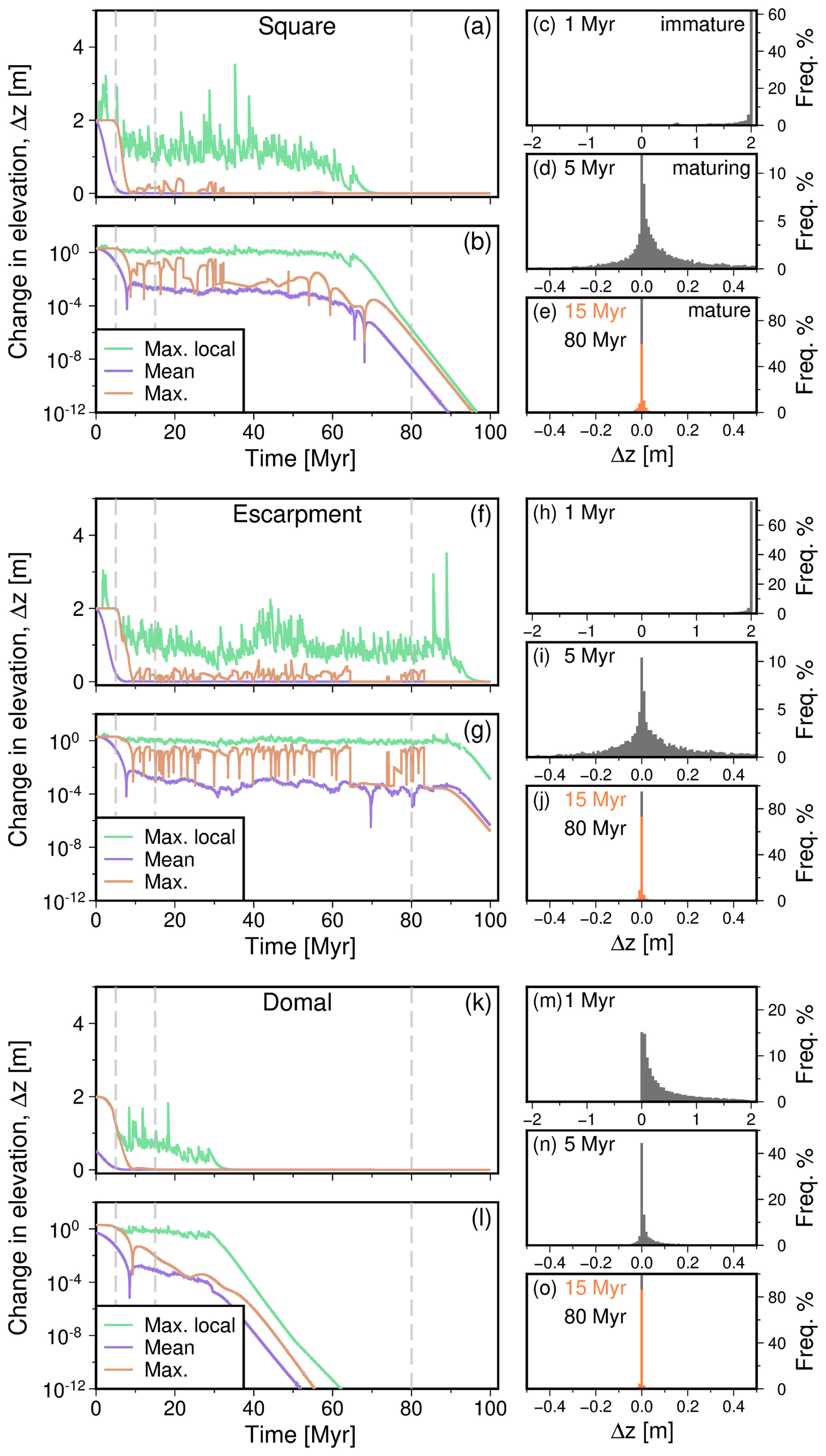
Figure 5 Identifying steady state landscapes. In each of these examples, white noise is only inserted in the starting condition, see scenario A in Fig. 3. (a) Evolution of changes in elevation between consecutive time steps (Δt=0.01 Ma) for the “square” landscape shown in Fig. 1d; green = maximum change in local elevation (Δz_α); purple and orange = change in mean elevation (Δz_β) and change in maximum elevation across the entire domain (Δz_γ), respectively (see Eqs. 9–11). Grey dashed vertical lines correspond to histograms shown in panels (c)–(e). (b) As (a), on logarithmic scale. (c) Histogram of elevation change, Δz, for all grid cells between 0.99 and 1 Myr. (d, e) As per (c), from 4.99→5 Myr, 14.99→15 Myr and 79.99→80 Myr, respectively. (f–j) As above for “escarpment” landscape shown in Fig. 1e. (k–o) As above for “domal” landscape shown in Fig. 1f.

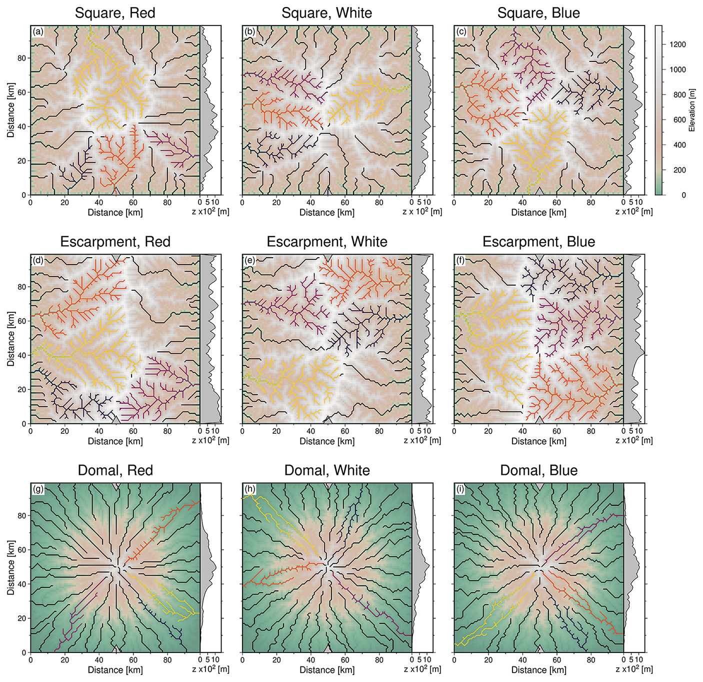
Figure 6 Steady state landscapes generated with different initial conditions. (a–c) Steady state “square” landscapes generated with red, white and blue initial conditions, respectively. Planforms of channels in the four largest drainage networks in each landscape are emphasised by the coloured lines. Main (longest) channels of 40 largest basins shown in black lines, plus the four longest coloured lines. Adjacent topographic transects are between grey triangles at x=50 km. (d–f) As above, for “escarpment” landscapes. (g–i) As above, for “domal” landscapes.

2.5 Mapping noise-specific geometries of landscapes

As Kwang and Parker (2019) discuss, planforms generated in simulations with noise inserted into starting conditions tend to be “burned” into simulated landscapes for the duration of model run time. This result is intuitive for models in which uplift rates tend not to vary as a function of time, or cannot outpace erosion (cf. O’Malley et al., 2021). This behaviour implies that long-lived planform geometries, at least at some scales, are specific to the distribution and particular arrangement of noise. We assess the consequences of inserting different distributions and specific arrangements of noisy topography on the geometries of emergent landscapes, their planforms and marginals by running multiple simulations (see e.g., Figs. 1, 6, 7).

We also make use of our model ensembles to assess the impact of different distributions and arrangements of noisy starting conditions on resulting drainage basin sizes. We extract the upstream drainage area from the outlet positions of the ten largest drainage basins in each “square” model of scenario A for 1000 simulations (ensembles 10–12) and show this in Fig. 8.

2.5.1 Establishing expectations (probabilities) of drainage network and divide geometries

Following Lipp and Roberts (2021), to develop statistical insights into the development of synthetic landscapes, we ran 1000 simulations for each landscape configuration within scenario A (i.e., “square”, “escarpment”, “domal”). The same distribution of noise, but different specific arrangements of topography (i.e., 1000 simulations initialised with different “seed” numbers) with amplitudes 0 to 1 m were used to define the initial conditions (model ensembles 10–18). To establish the propensity of cells within landscapes to host rivers, cells with upstream drainage areas > 5 × 10⁷ m² were extracted from each model. The probability of a river being in a cell is calculated by dividing the number of times a cell met this criteria by the total number of simulations (i.e., $N/\mathrm{1000}$), which results in a probabilistic drainage map (Fig. 9). These maps also help to establish expected locations of drainage divides, i.e., where calculated probability is low. Similar maps are shown for 100 “square” landscapes generated in scenarios B and C in Fig. S6.

The spectral characteristics of the synthetic landscapes can be assessed by transforming them into the frequency domain using Eqs. (3) and (7) (see Fig. 10). It is also straightforward to extract other geometric properties from the landscapes (e.g., longitudinal river profiles, hypsometry, channel length-area relationships) that can be directly compared or used to calculate geomorphic metrics that can be compared in turn (Fig. 11).

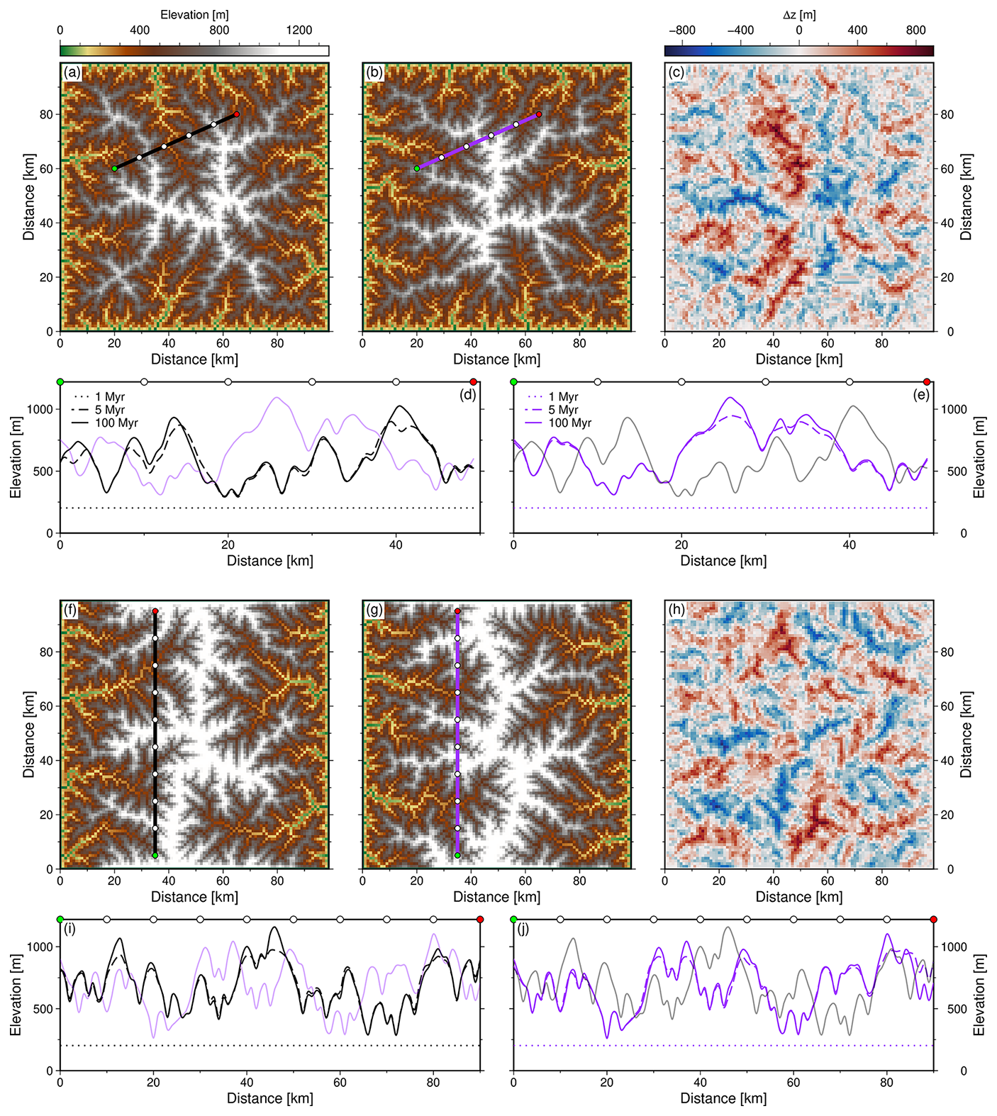
Figure 7 Differences in elevations and drainage network planforms due solely to changing arrangements of initial noise. (a–b) Steady state “square” landscapes (at 100 Myr) generated with the same uplift rate histories, boundary conditions, and distributions (but different arrangements) of white noise. (c) Landscape in panel (a) subtracted from that in panel (b). (d) Black dotted, dashed, solid lines = elevation along transect indicated in panel (a) at 1, 5 and 100 Myr. Purple line = landscape at 100 Myr along transect indicated in panel (b). (e) as for (d) for transects shown in panels (b) and (a). (f–j) Same as panels (a)–(e) for “escarpment landscapes”.

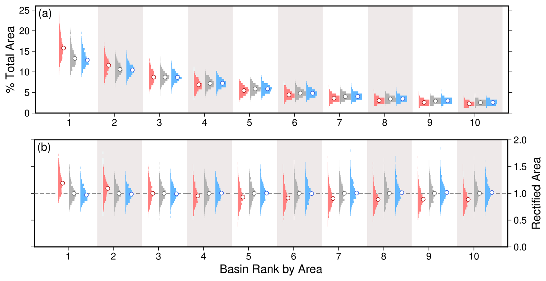
Figure 8 Variability of drainage areas due to noise. (a) Distributions of maximum upstream drainage area for the 10 largest drainage basins of 1000 simulations for red, white, and blue noise initial conditions (i.e., scenario A, ensembles 10–12). White closed circles show median values of drainage area as a proportion of total landscape area. Cumulative median areas sum to 64.4 %, 63.5 %, and 63.0 % for red, white, and blue noise respectively. (b) Data shown in (a) are divided by the white noise median values of drainage area in each respective basin.

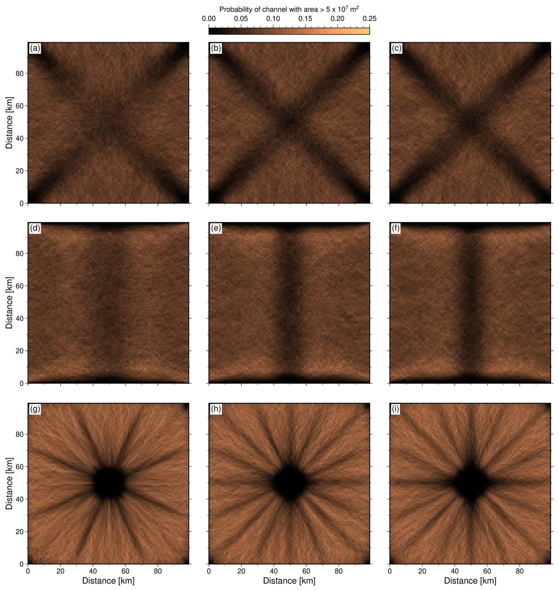
Figure 9 Probability of drainage within landscapes generated by different arrangements of initial noise. (a–c) Colours indicate probability of a grid cell in 1000 “square” landscapes containing a channel with upstream drainage area > 5 × 10⁷ m² generated with initial red (a), white (b), or blue (c) noise. (d–f) As above, for “escarpment” landscapes, and (g–i) for “domal” landscapes. Examples of individual landscapes that feature in this suite are shown in Fig. 6. Associated power spectra are shown in Fig. 10.

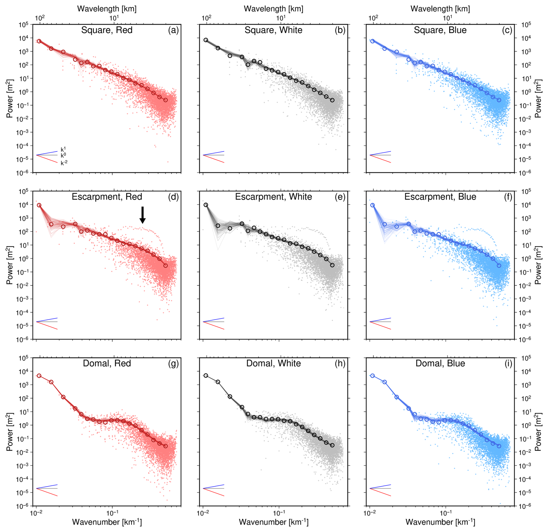
Figure 10 Spectral (two-dimensional Fourier) analysis of steady state landscapes generated with noise in the initial condition. (a) Small red dots = power at positive frequencies from the two-dimensional Fourier transform collapsed into one dimension for a single “square” landscape generated with a red noise initial condition (see body text for details). Open circles = mean power within logarithmically equalled spaced bins (see Eq. 8). Thin lines show the mean values for the other 99 models with same distribution but different arrangement of initial noise. (b–c) As per (a), for a steady state landscape generated with a white noise (b), and blue noise (c) initial condition. (d–f) As per (a–c) for the “escarpment” landscapes such as that shown in Fig. 1d. Arrow indicates power for regions on north and south boundaries. (g–i) Power spectra for “domal” landscapes (e.g., Fig. 1e).

2.6 Geomorphic metrics

We examine the impact of noise on widely used geomorphic metrics. The metrics extracted from landscapes in this study include: concavity indices, erosional parameter values and uplift rates from slope-area and χ (chi) analyses. In most landscape evolution models the typical order of a single time step, which we follow, is add noise (if desired) → uplift → flow routing → erode. For efficiency, slopes and drainage areas are calculated as part of the flow routing step. However, an obvious issue is that we want to calculate metrics for steady state landscapes, which requires knowledge of landscape geometries once erosion has been performed. Therefore, just prior to extracting metrics (i.e., at time step N=100 Myr) we run a single additional flow routing step.

Hack exponents are calculated from channel lengths and basin areas. Hypsometry is calculated using elevations and cell areas. Longitudinal river profiles are extracted from the synthetic landscapes using a version of the code within the ChannelProfiler component of Landlab (modified for data manipulation and visualisation). We note that metrics are often derived, via slope-area or χ analyses, for instance, from profiles alone.

2.6.1 Slope-area analysis

Expectations of power law scalings of channel slope and upstream areas were discussed by Gilbert (1877), and later quantified in a few settings by Hack (1957), Morisawa (1962) and Flint (1974), and subsequently by many others. Slope-area analysis remains a widely used tool to estimate uplift rates and erosional parameter values (e.g., Schoenbohm et al., 2004; Kirby and Whipple, 2012; Adams et al., 2020; Marder and Gallen, 2023). It is typically applied to information about local changes in slope, $\partial z\left(x\right)/\partial x$, and upstream drainage areas, A(x), extracted from the longitudinal profiles of individual rivers, where x here indicates streamwise distance. There are many explanations of the approach in previously published work (see e.g., Tarboton et al., 1989; Montgomery and Foufoula-Georgiou, 1993; Kirby and Whipple, 2001). For completeness we summarise it as follows. If a river is assumed to be at topographic steady state, $\partial z/\partial t$ = 0, κ = 0, and there are no additional sources of elevation (e.g., noise), the one dimensional version of Eq. (1), predicting evolution of the longitudinal profile of the river,

$$\begin{array}{}\text{(12)}& {\displaystyle \frac{\partial z\left(x\right)}{\partial t}}=-KA(x{)}^m{\left({\displaystyle \frac{\partial z}{\partial x}}\right)}^n+U,\end{array}$$

can be rearranged such that

$$\begin{array}{}\text{(13)}& \left|{\displaystyle \frac{\mathrm{d}z}{\mathrm{d}x}}\right|={\left({\displaystyle \frac{U}{K}}\right)}^{\frac{\mathrm{1}}{n}}A(x{)}^{-\frac{m}{n}}.\end{array}$$

By substituting k_s (the “channel steepness index”) for $(U/K{)}^{\frac{\mathrm{1}}{n}}$, and θ (“concavity index”) for the exponent ratio $m/n$, Eq. (13) can be rewritten as

$$\begin{array}{}\text{(14)}& \log \left(S\right)=\log \left(k_{\mathrm{s}}\right)-\mathit{\theta }\log \left(A\right).\end{array}$$

Equation (14) takes the form of a straight line in a plot of log (S) against log (A), with gradient θ, and log (k_s) at the y-intercept. In turn, because we know the values of n and K in the experiments we run, we can, in principle, recover the values of uplift rate and erosional parameter m,

$$\begin{array}{}\text{(15)}& U={k_{\mathrm{s}}}^{n}K,m=\mathit{\theta }n.\end{array}$$

The black line in Fig. 11e shows the analytical relationship (from Eq. 14) between slope and area expected for all rivers within steady state landscapes generated with “block” uplift (see Fig. 4: “square”, “escarpment”) in this study given the values of erosional parameters and uplift rate used. We restrict slope-area analysis of river profiles extracted from the two-dimensional landscapes to cells with upstream drainage areas > 4 km², a value often used in studies of real landscapes as indicative of overland flow (e.g., Whipple and Tucker, 1999; Roberts and White, 2010). Slope is calculated between adjacent cells in the streamwise distance downstream.

2.6.2 Chi analyses

Metrics estimated from slope-area analysis can be extremely sensitive to noise and thus calculated parameter values can be highly unstable (see e.g., Roberts et al., 2012b; Smith et al., 2022). This result is unsurprising because even small amounts of noise can dramatically change local slopes. Fortunately, a variety of integral-based techniques exist that avoid the need for differentiation of elevations when attempting to recover information from fluvial landscapes (e.g., erosional parameter values, uplift rates; see e.g., Harkins et al., 2007; Pritchard et al., 2009; Roberts and White, 2010; Roberts et al., 2012a; Perron and Royden, 2013).

Here, we focus on examining impact of noise on geomorphic metrics calculated using the widely used “χ” (chi) analysis (Royden et al., 2000; Harkins et al., 2007; Perron and Royden, 2013). Like slope-area analysis, χ-analysis can, in principle, be used to estimate uplift rates and values of erosional parameters from the geometries of longitudinal river profiles providing certain assumptions hold. There are many published explanations of the approach available (see e.g., Perron and Royden, 2013; Mudd et al., 2014, 2018; Smith et al., 2022; Marder et al., 2023). For completeness, we summarise it as follows. First, Eq. (13) is rearranged and integrated in the upstream direction such that

$$\begin{array}{}\text{(16)}& z\left(x\right)=z_{\mathrm{b}}+\underset{x_{\mathrm{b}}}{\overset{x}{\int }}{\displaystyle \frac{k_{\mathrm{s}}}{A(x{)}^{\frac{m}{n}}}}\mathrm{d}x,\end{array}$$

where z is elevation, x_b is a downstream position on the channel often assumed to be base level (though not always), with elevation z_b. A reference drainage area A_∘ (here =1 m²) is often incorporated, such that

$$\begin{array}{}\text{(17)}& z\left(x\right)=z_{\mathrm{b}}+{\displaystyle \frac{k_{\mathrm{s}}}{A_{\circ }^{\frac{m}{n}}}}\underset{x_{\mathrm{b}}}{\overset{x}{\int }}{\displaystyle \frac{A_{\circ }^{\frac{m}{n}}}{A(x{)}^{\frac{m}{n}}}}\mathrm{d}x.\end{array}$$

Thus χ is defined,

$$\begin{array}{}\text{(18)}& \mathit{\chi }\left(x\right)=\underset{x_{\mathrm{b}}}{\overset{x}{\int }}{\left({\displaystyle \frac{A_{\circ }}{A\left(x\right)}}\right)}^{\frac{m}{n}}\mathrm{d}x.\end{array}$$

Making use of Eq. (15),

$$\begin{array}{}\text{(19)}& z\left(x\right)=z_{\mathrm{b}}+{\displaystyle \frac{k_{\mathrm{s}}}{A_{\circ }^{\frac{m}{n}}}}\mathit{\chi }\left(x\right)=z_{\mathrm{b}}+{\left({\displaystyle \frac{U}{K{A}_{\circ }^m}}\right)}^{\mathrm{1}/n}\mathit{\chi }\left(x\right).\end{array}$$

Various techniques exist to find the optimal values of $m/n$ from the construction of z(χ) profiles (e.g., Perron and Royden, 2013; Mudd et al., 2014; Hergarten et al., 2016; Mudd et al., 2018; Gailleton et al., 2021). If the landscape is at steady state then elevation is expected to be a linear function of χ. By systematically sweeping $\mathrm{0}<m/n\le \mathrm{1}$, the optimal value can be identified, i.e., as one that results in the z(χ) profile with the highest linear correlation coefficient, R² (see e.g., Perron and Royden, 2013). In the experiments run in this study, we of course know the true values of m and n. As Fig. S4 shows, if an incorrect value of $m/n$ is assumed, z(χ) profiles are not linear. Correlation coefficients are calculated for the main channel in each simulation to identify the “optimal” value of $m/n$ as if we were studying a real landscape for which no independent information about the erosional parameter values exists. Once armed with an optimal value for $m/n$ it is straightforward to estimate the uplift rate from the slope of the z(χ) profile (because we know the values of n=1 and K here),

$$\begin{array}{}\text{(20)}& U=K{A}_{\circ }^m{\displaystyle \frac{\mathrm{d}z}{\mathrm{d}\mathit{\chi }}}.\end{array}$$

Figure 11f shows an example of a relationship between χ and elevation for the main channel and tributaries of the largest drainage network in a single simulation.

2.6.3 Hack exponent

Hack's law is an empirical relationship between the length of rivers and their upstream drainage areas, both of which are straightforward to extract from synthetic landscapes and digital elevation data. It has been used to relate changes in channel sinuosity to basin shapes, to develop an understanding of fractal (scale-dependent) characteristics of basins, and of energy expenditure in drainage basins, for example (Langbein, 1947; Hack, 1957; Robert and Roy, 1990; Ijjasz-Vasquez et al., 1993; Rigon et al., 1996; Turcotte, 1997; Willemin, 2000). The law can be expressed as

$$\begin{array}{}\text{(21)}& L=C{A}^h\mathrm{thus}\log \left(L\right)=\log \left(C\right)+h\log \left(A\right),\end{array}$$

where L is the length of the longest river in a basin, A is upstream drainage area, and C and h are known as the Hack coefficient and exponent, respectively. Their values can be estimated from the respective intercept and slope of regressed log (L) and log (A) data. We show how noise impacts the values of Hack exponents calculated from the maximum lengths and upstream drainage areas of the longest channels in the forty largest drainage basins (by area) in each model run.

2.6.4 Hypsometry

Hypsometry summarises area-elevation relationships of a landscape, including topography not necessarily incorporated into the other geomorphic metrics examined (see e.g., Langbein, 1947; Strahler, 1952, 1957; Harrison et al., 1983; Lifton and Chase, 1992; Willgoose and Hancock, 1998; Hurtrez et al., 1999; Montgomery et al., 2001). We calculate hypsometry for the entire domain of each steady state landscape by generating normalised cumulative density functions (the simple algorithm used is available; see the Code and Data Availability statement). Hypsometry is also produced for select landscapes during their evolution (e.g., Fig. 11g).

We have now introduced each of the geomorphic metrics extracted from synthetic landscapes in this study. Our primary aim is to assess how changing the colour, amplitude, timing, and arrangement of noise affects these metrics. We synthesise results for each scenario as follows.

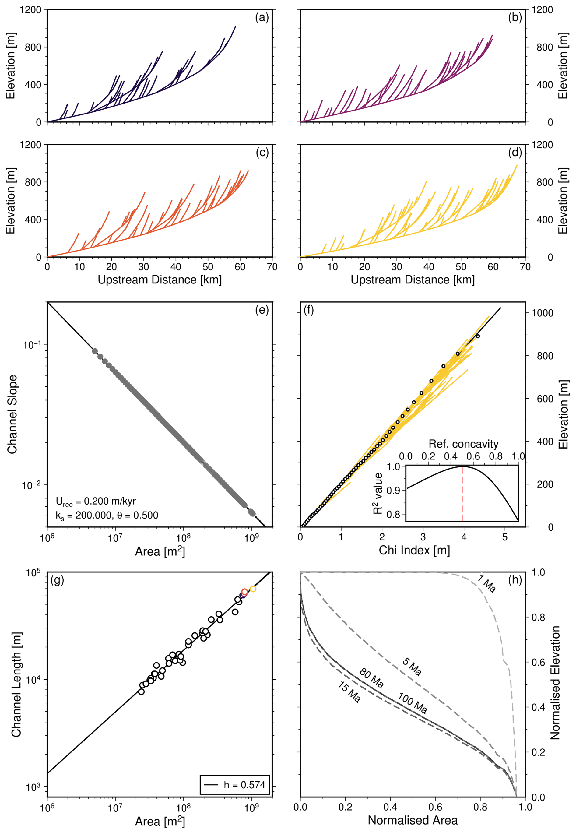
Figure 11 Geomorphic metrics for an example “square” landscape generated with white noise only in the initial condition. All metrics are for the steady state landscape (at 100 Myr) shown in Fig. 6b unless otherwise indicated. (a–d) Longitudinal profiles of rivers, including tributaries, within four largest drainage basins shown in Fig. 6b. (e) Grey points show slope-area relationship for grid nodes of rivers in four largest basins with drainage areas exceeding 4 km². Black line = linear regression: calculated intercept = k_s (steepness index); U_rec= recovered uplift rate; slope = $\mathit{\theta }=m/n$ (concavity index). True values, used to generate LEM: U=0.2 m kyr⁻¹, θ=0.5. See body text for details. (f) Yellow = χ-elevation profiles for the main channel and tributaries of the largest drainage basin (d); open circles = main channel. Inset shows R² values for different assumed concavity indices for main channel; red dashed line = true value. Black solid line in main panel illustrates linear relationship for θ=0.5. (g) Coloured/black circles show maximum length-drainage area relationships for longest rivers from four/forty largest drainage basins, respectively. h = Hack exponent. (h) Hypsometry (i.e., landscape area-elevation relationships) at 1, 5, 15, 80 and 100 Ma.

3 Results

3.1 Scenario A: noise only inserted into the initial condition

3.1.1 Verification of topographic steady state

The boundary conditions and uplift rates – producing “square”, “escarpment”, or “domal” landscapes in this study – influence the precise time taken to reach steady state. Histograms shown in Fig. 5 illustrate that, for the erosional model used in this study, with noise only inserted into initial conditions, landscapes are immature and topographic change is driven by the imposed uplift until ca. 1 Myr. By 5 Myr, the landscapes are maturing as drainage networks develop; topographic change is largely centred around zero by this time. By 15 Myr drainage networks have matured such that erosion rates balance the imposed uplift rates across most of the domain. For most intents and purposes these landscapes can be regarded as being at steady state at this time. However, we note that true numerical steady state is achieved where topographic change within a single time-step across all cells is zero within computer precision, which is typically achieved by 40–90 Myr.

3.1.2 Spectral power of initial, sink-filled, and steady state landscapes

Figure 1c shows examples of the spectral content of single models. It demonstrates how landscapes with initial white noise (ϕ∝k⁰) quickly “redden” due to sink-filling, which reduces local roughness, resulting in such sink-filled landscapes having pink noise ($\mathit{\varphi }\propto k^{-\mathrm{1}}$) characteristics. Figure 2d shows the spectral content of 100 initial conditions for each distribution of noise (red, white, blue) used in this study.

Examination of the power spectra of evolving landscapes shows that the spectral signature of all (red, white, blue) initial noise conditions with amplitude 0–1 m evolve to have red noise characteristics within 2 Myr of model run time ($\mathit{\varphi }\propto k^{-\mathrm{2}}$). We attribute spectral reddening of topography in these landscape evolution models to the smoothing effects of sink-filling and erosion, and the imposed uplift. Figure 10 shows radially-averaged power spectra for typical steady state landscapes in ensembles 1–9. The escarpment landscapes (ensembles 2, 5, 8) contain above-average spectral power at a few intermediate to high wavenumbers (${\mathrm{10}}^{-\mathrm{1}}\le k\le \mathrm{5}\times {\mathrm{10}}^{-\mathrm{1}}$ km⁻¹), highlighted with the black arrow in Fig. 10d. This pattern is attributed to the high elevations at the closed north and south boundaries of these landscapes. The domal landscapes exhibit a flattening in the power spectrum at intermediate wavenumbers ($\mathrm{5}\times {\mathrm{10}}^{-\mathrm{2}}\le k\le \mathrm{1}\times {\mathrm{10}}^{-\mathrm{1}}$ km⁻¹). The flattening corresponds to a white noise signal at these wavenumbers. We attribute this spectral power to the areas of low elevation (few meters) between the uplifted dome and the edge of the domain.

Overall, Fig. 10 shows that whilst landscape configuration can influence the details of the power spectrum, the steady state landscapes produced in this study tend to exhibit red noise characteristics and are insensitive to the colour of noise used to generate the initial condition.

3.1.3 Impact of noise on geometries and planforms

In contrast, Fig. 6 illustrates how those initial conditions can lead to very different drainage planforms. This result emerges even for landscapes that are generated with the same erosional model parametrisations and uplift histories. Figure 7 extends this demonstration by showing how different arrangements of the same distribution of noise (e.g., white) in the initial condition results in formation of very different drainage planforms. Inevitably, the dissimilarity of planform arrangements is consistent with elevations being very different locally, resulting in substantial differences in the positions of valleys and interfluves. These differences are illustrated using topographic transects from identical locations in the two landscape models shown in Fig. 7.

As a further demonstration of the impact of noisy initial conditions on the geometries of landscapes, Fig. 8 shows drainage area of each of the 10 largest fluvial networks in the 3000 simulations generated with either red, white, or blue noise as a percentage of the total area of the model domain. The are ordered by rank: largest to smallest drainage area. Landscapes initialised with red noise tend to create, on average, fewer, larger drainage basins. The upstream area of the largest drainage basin in a landscape initialised with red noise can be up to 2 times that of the median white noise equivalent, and on average is approximately 20 % larger. A consequence is that smaller drainage basins (rank 4 and below) in landscapes initialised with red noise are smaller than their white and blue noise counterparts. Drainage basins in landscapes generated by white and blue noise conditions are similar in size to each other.

Figure 9 shows calculated probabilities of channel locations for steady state landscapes generated with different distributions of initial noise. We emphasise three features of interest in the probability maps of “square” landscapes (Fig. 9a–c). First, all three distributions of noisy initial conditions have regions of low probability within a “cross” that extends from the four corners of the domain to its centre. Secondly, in between those regions the probability of drainage is broadly equal, and relatively high. Thirdly, landscapes with red noise initial conditions (panel a) have a more uniform probability of drainage across the domain. The escarpment landscapes initialised with red noise also have a higher probability of drainage across the domain than those initialised with white or blue noise (Fig. 9d–f).

The domal landscapes exhibit probabilistic drainage patterns with a radial “spoke” pattern for all three colours of noise. We interpret this pattern as being a consequence of the interaction of D8 flow routing on a Cartesian raster grid and the distribution of inserted uplift. We suggest that the lower number of spokes for landscapes generated with red noise initial conditions are a result of longer wavelength topographic roughness reducing the propensity for a flowpath to be diverted locally as frequently as they are for white or blue noise. In other words, channels in a landscape initialised with red noise are more likely to drain along a continuous azimuth without being interrupted by local topographic roughness. We note that the structure of probability in these maps is similar to drainage networks produced in models with no added noise (see Supplement Fig. S2).

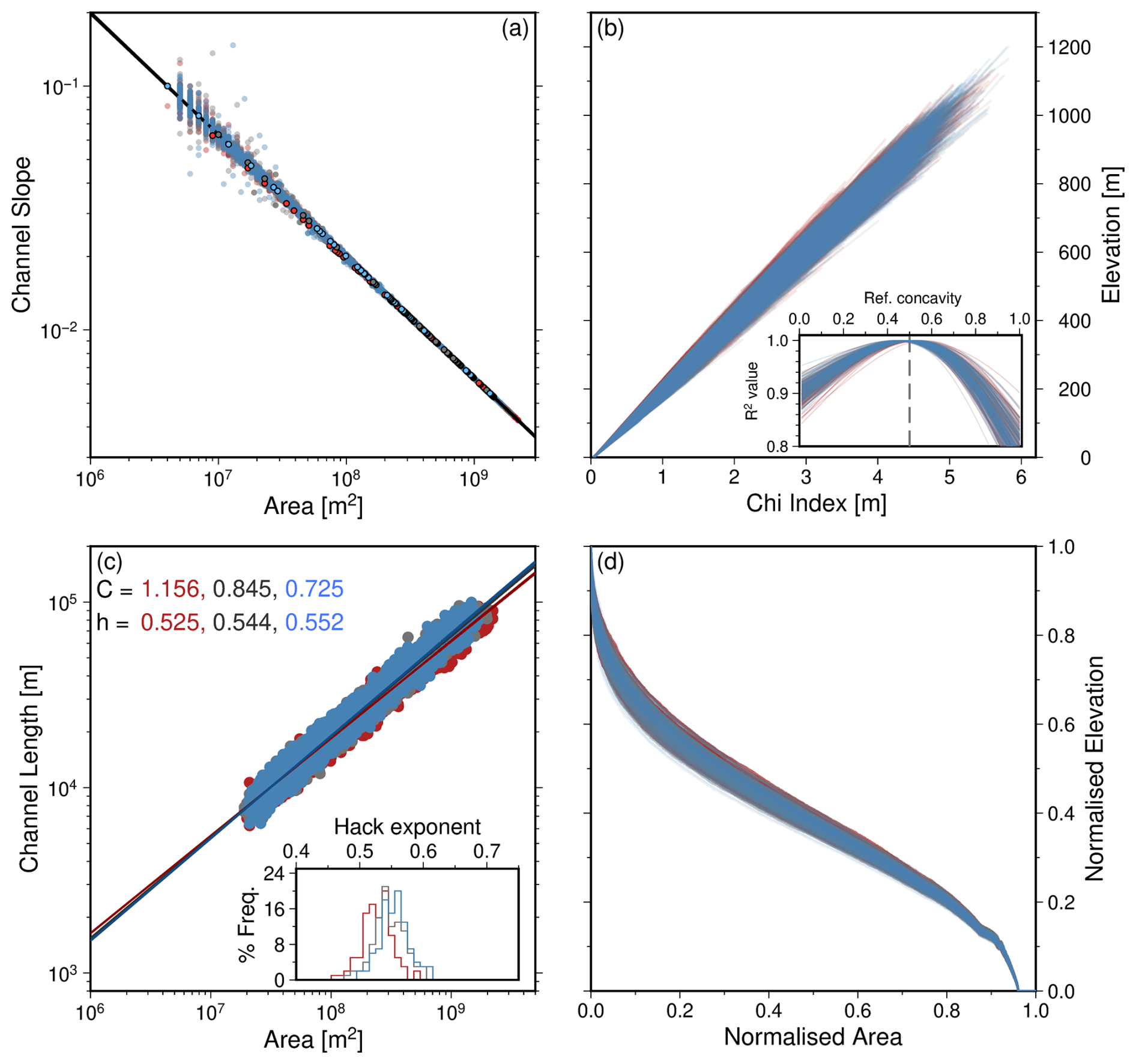
Figure 12 Comparing geomorphic metrics from “square” steady state landscapes initialised with red, white or blue noise. Each panel shows metrics from 100 landscapes initialised with red, white or blue noise. (a) Upstream drainage area vs. channel slope for all grid cells in rivers of four largest drainage basins with drainage area > 4 km²; black line = linear regression. Outlined circles show examples of relationships for the main channel in the largest drainage network in single, typical, simulation for each colour of noise. (b) Elevation as a function of χ for the main channel and tributaries of the largest drainage basin in each simulation, produced using θ=0.5. Inset shows the R² value of different reference concavities. Dashed line marks true value of 0.5 used to parametrise models. (c) Maximum upstream drainage area vs. maximum channel length for the longest (trunk) channels in the forty largest drainage networks in each landscape. Inset histogram shows Hack exponent for the 4000 rivers generated for each colour of noise. (d) Hypsometries of the 300 landscapes.

Figure 13 Geomorphic metrics of steady state “escarpment” landscapes initialised with red, white or blue noise. See Fig. 12 for extended notation.

3.1.4 Slope-area analysis

Slope-area data shown in Figs. 11e, 12a and 13a are clustered around a single line with a slope and intercept that permit reliable uplift rates, U_SA, and $m/n$ ratios (θ_SA) to be recovered (Eq. 15). These results demonstrate the utility of slope-area analysis for landscapes that are demonstrably at topographic steady state and subject to spatially invariant uplift; the “square” and “escarpment” landscapes we study. Lines of best fit are shown in Figs. 12a and 13a for each of the 3 × 100 simulations generated with 0–1 m of red, white or blue noise. They are largely indistinguishable from each other, demonstrating the insensitivity of slope-area relations to the colour of noise in the initial conditions. We note that changing the amplitude of noise increases the spread of calculated U_SA and θ_SA (Fig. S5). However, changing the amplitudes of initial noise, even by many orders of magnitude, has a small impact (few percent compared to true values) on the recovered values of U_SA and θ_SA.

3.1.5 χ analysis

Figures 11f, 12b and 13b show z(χ) profiles for the main channel and tributaries of the single largest drainage basin for simulations in which uplift rate is spatially invariant (“square” and “escarpment”). Results are shown for each of the 100 simulations generated with red, white or blue noise initial conditions. In theory, z(χ) profiles in such steady state landscapes should be straight and collinear, i.e., collapse to a single line (see Section 2). Whilst individual profiles are linear, we demonstrate that when the models are initialised with noisy conditions, families of profiles do not collapse to a single line, even when they have the same distribution of noise in their initial conditions.

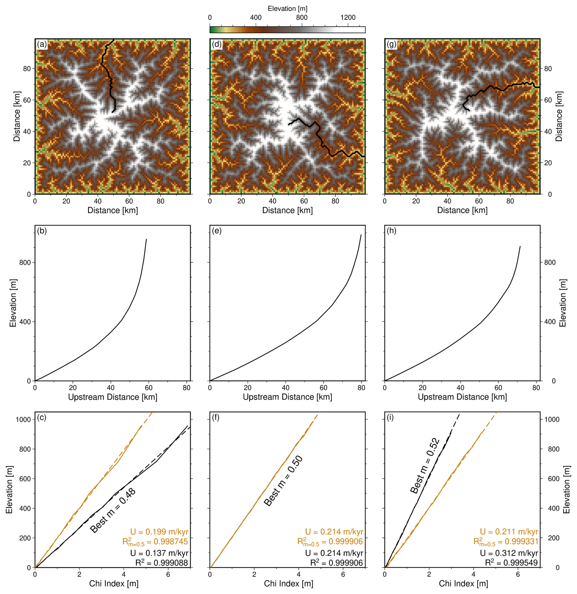
Figure 14 Impact of noise on recovered uplift rates from z(χ). (a) Topography and planform of longest single river channel for a steady state landscape initialised with 0–1 m white noise (scenario A). (b) Longitudinal profile of largest river channel. (c) Longitudinal profile transformed into χ space (see Eqs. 16–19) using a best-fitting (highest R²) reference concavity value of 0.48 (black solid line) and the true $m/n$ value of 0.5 (orange solid line). Dashed black and orange lines show linear regressions. The slope of these lines, $\mathrm{d}z/\mathrm{d}\mathit{\chi }$ is used to calculate an uplift rate (see Eq. 20). (d)–(f) and (g)–(i) show two additional landscapes, longitudinal profiles, and z(χ) profiles for models in scenario A with different arrangements of white noise and different best-fitting reference concavity values.

The inset panels in Figs. 11f, 12b and 13b show R² values for the suite of z(χ) profiles generated by systematically testing different concavity values (θ_χ; see Sect. 2). Highest R² values are generated when $\mathrm{0.4}\le {\mathit{\theta }}_{\mathit{\chi }}\le \mathrm{0.6}$ (note: actual value used to produce the landscapes is 0.5). These results highlight the variability in best-fitting χ transformations introduced by different noisy initial conditions.

Having established that different colours and arrangements of noise in initial conditions contribute to uncertainty in calculated best-fitting concavity, Fig. 14 demonstrates the impact of using the best-fitting values on calculated uplift rates. This test mimics calculation of θ and U from χ-transformation of rivers in the real world. In this demonstration the rivers with the largest upstream drainage area were extracted from three typical landscapes initialised with different arrangements of white noise (scenario A: ensemble 1). Each longitudinal river profile is transformed into a z(χ) profile using the best-fitting value of concavity. R² values for each θ_χ value are shown. In the cases where the best-fitting reference concavity ≠ 0.5 (i.e., the true value), uplift rates recovered from the slope of the regression line (see Eq. 20) significantly differ – by more than 50 % when amplitudes of initial noise are 0–1 m – from the true value of 0.2 m kyr⁻¹. These results demonstrate that even though chosen values of θ_χ may result in z(χ) profiles with high R² values (>0.99), they can yield inaccurate and misleading estimates of uplift rates. The instability of calculated U_χ arises because of its sensitivity to the derivative, $\mathrm{d}z/\mathrm{d}\mathit{\chi }$ (see Eq. 20), and the sensitivity of $\mathrm{d}z/\mathrm{d}\mathit{\chi }$ to noise and the way in which it impacts the geometries of landscapes.

3.1.6 Length-area relationships

Relationships between maximum channel lengths and upstream drainage areas are shown in Fig. 11g (black circles) for the main channels within the forty largest basins extracted from a typical “square” landscape initialised with white noise. A best-fitting non-linear regression, generated using Eq. (21), is shown, and yields a Hack exponent value, h (slope of regression in log-log space), of 0.574.

Figures 12c, 13c and 15c collate lengths and areas for the main channels in the forty largest drainage basins for each ensemble in scenario A. The non-linear regression is shown for each ensemble. The regressions are similar for landscapes initialised with white and blue noise, However, a shallower gradient (and hence lower h) is required for landscapes initialised with red noise. Each inset panel in these figures show histograms of Hack exponent values calculated for each model from its forty longest rivers. They demonstrate the variability in Hack exponent values: $\mathrm{0.4}\le h\le \mathrm{0.75}$, with h values in the landscapes generated with red noise initial conditions tending to be slightly lower than those for the white and blue noise initial conditions.

Figure 16a–c demonstrates that the amplitude of initial noise has limited influence on the distributions of Hack exponents at the range of amplitudes tested (0.002 to 200 m). Landscapes initialised with different amplitudes of red, white or blue noise have broadly consistent trends. For instance, the 25th and 75th percentile, and median show little variation between ensembles 1, 4 and 7 (Fig. 16). These results demonstrate that the distribution of Hack exponent values largely do not depend on the amplitude of initial noise. They all show considerable variance arising from noisy initial conditions.

3.1.7 Hypsometry

The history of hypsometry for a single landscape is shown in Fig. 11h. A large proportion of the landscape has relatively high elevations early in its evolution, whilst fluvial networks are forming. As the landscape matures, an increasing proportion of its area is at lower elevations. Figures 12d, 13d and 15d show the hypsometries of steady state landscapes within scenario A. We emphasise two features. First, changing the arrangement of specific distributions of noise (i.e., red, white, blue) generates up to approximately 5 % variability in the hypsometry, but the shape of the hypsometric curves remain similar. This result is expected as hypsometry is largely insensitive to the age or maturity of landscapes once they approach steady state. Secondly, there is little difference between the hypsometries of the landscapes initialised with red, white or blue noise once they reach steady state. Figure 16d–f show the hypsometries for ensembles 1, 4 and 7 in which amplitudes of noise in the initial conditions is systematically varied between 0.002 and 200 m. These results show that hypsometries of steady state landscapes are largely insensitive to the amplitudes of initial noise.

3.1.8 Spatially variable uplift

We now draw attention to the results for domal landscapes (Fig. 15). Unsurprisingly, they tend to reach steady state earlier than “escarpment” or “square” landscapes generated with the same erosional model (Fig. 5k–o). Given that a fundamental assumption in slope-area and χ analyses (i.e., that uplift is spatially invariant) no longer holds, it is also unsurprising that the results shown in Fig. 15a–b have considerably more scatter than the equivalent panels in Figs. 12 and 13. Decreases in slope as a function of upstream area are not linear, clearly departing from the analytical solutions expected when uplift is spatially invariant. z(χ) profiles are not (col)linear when produced using the true concavity value of 0.5. Instead, the value of θ_χ that best linearised these profiles is close to 1. Therefore, it is also unsurprising that calculated values of uplift rate and concavity indices are wrong when uplift varies spatially. We discuss alternative approaches to recovery of uplift histories and erosional parameter values in Sect. 4.

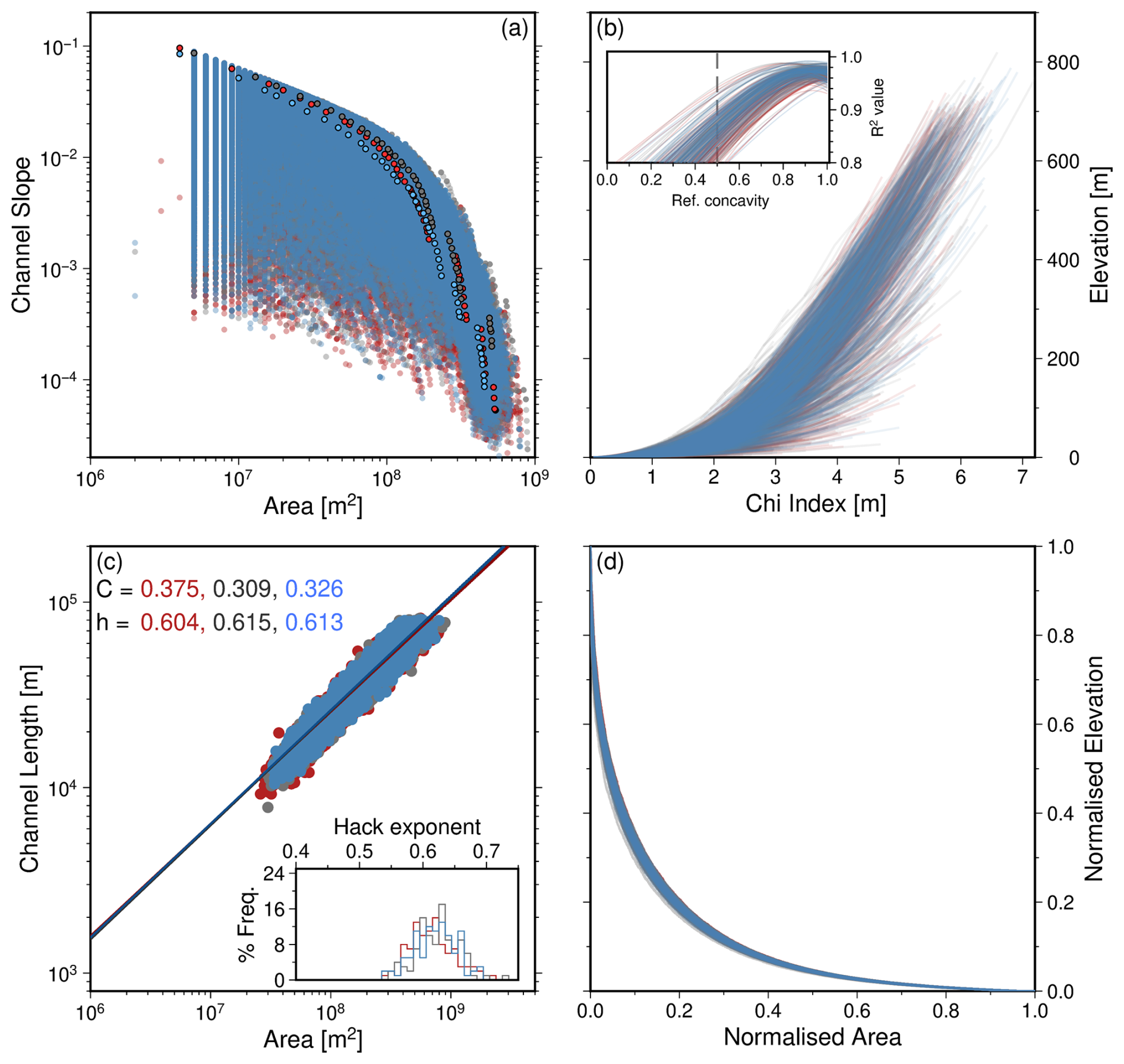
Figure 15 Geomorphic metrics of steady state “domal” landscapes initialised with red, white or blue noise. (a) Coloured circles with black outline show slope-area relationships for the main channel in the largest drainage network in single, typical, simulations initialised with red, blue or white noise. (b–d) See Fig. 12 for notation.

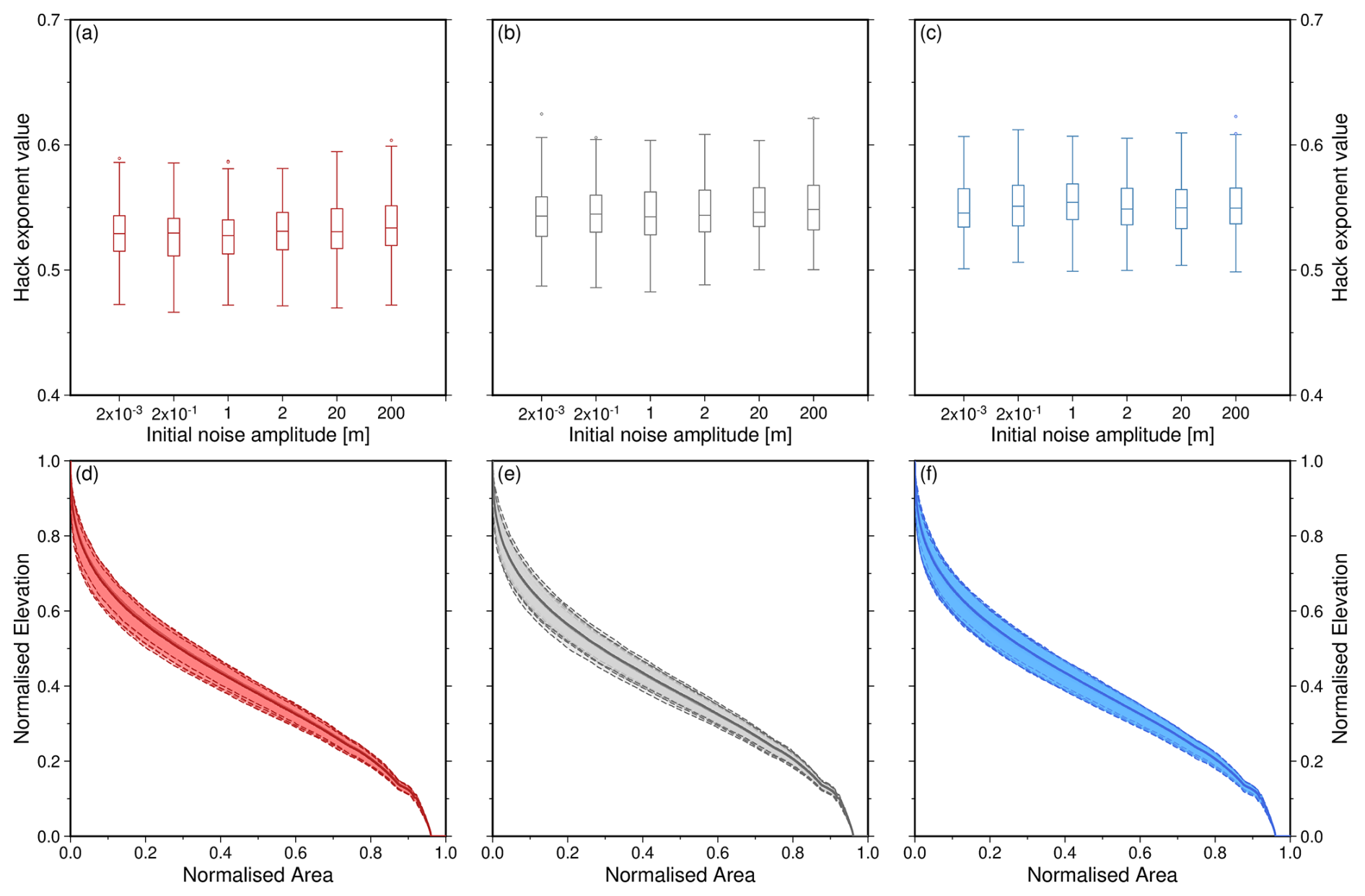
Figure 16 Impact of amplitude of initial red, white or blue noise on geomorphic metrics recovered from steady state “square” landscapes. Each box-and-whiskers plot shows results for M=100 landscapes generated with annotated initial noise of indicated colour. Whiskers = 1.5×IQR, or maxima/minima if higher/lower; dots = fliers. (a–c) Range in Hack exponent. (d–f) Solid lines = median hypsometries; filled areas shows range for M=100 landscapes of each amplitude of initial noise, bounded by dashed lines.

3.2 Scenario B: quenched noise

3.2.1 Drainage planforms and steady state

The impact of adding quenched noise to the morphometry of a single simulated landscape is shown in Fig. 17a–b. In this typical example, both landscapes are initialised with identical noisy starting conditions and evolve under the same forcing except for the identical (quenched) noise that is added at each time step to the model shown in panel (a). The landscape with quenched noise contains a larger proportion of higher elevations, as expected due to the additional noise. The mean elevation of added noise is 0.5 m per time step (10 kyr). In essence, the addition of quenched noise in this way may be considered as a noisy but spatially constant uplift rate of 0.2–0.3 m kyr⁻¹, with a mean uplift rate of 0.25 m kyr⁻¹. Thus, added noise contributes mean cumulative uplift of 5 km by 100 Myr. In comparison, when added noise has a mean elevation of 0 m per time step, the quenched noise landscape has elevations which are similar to that of the landscape in Scenario A (see Supplement Fig. S9).

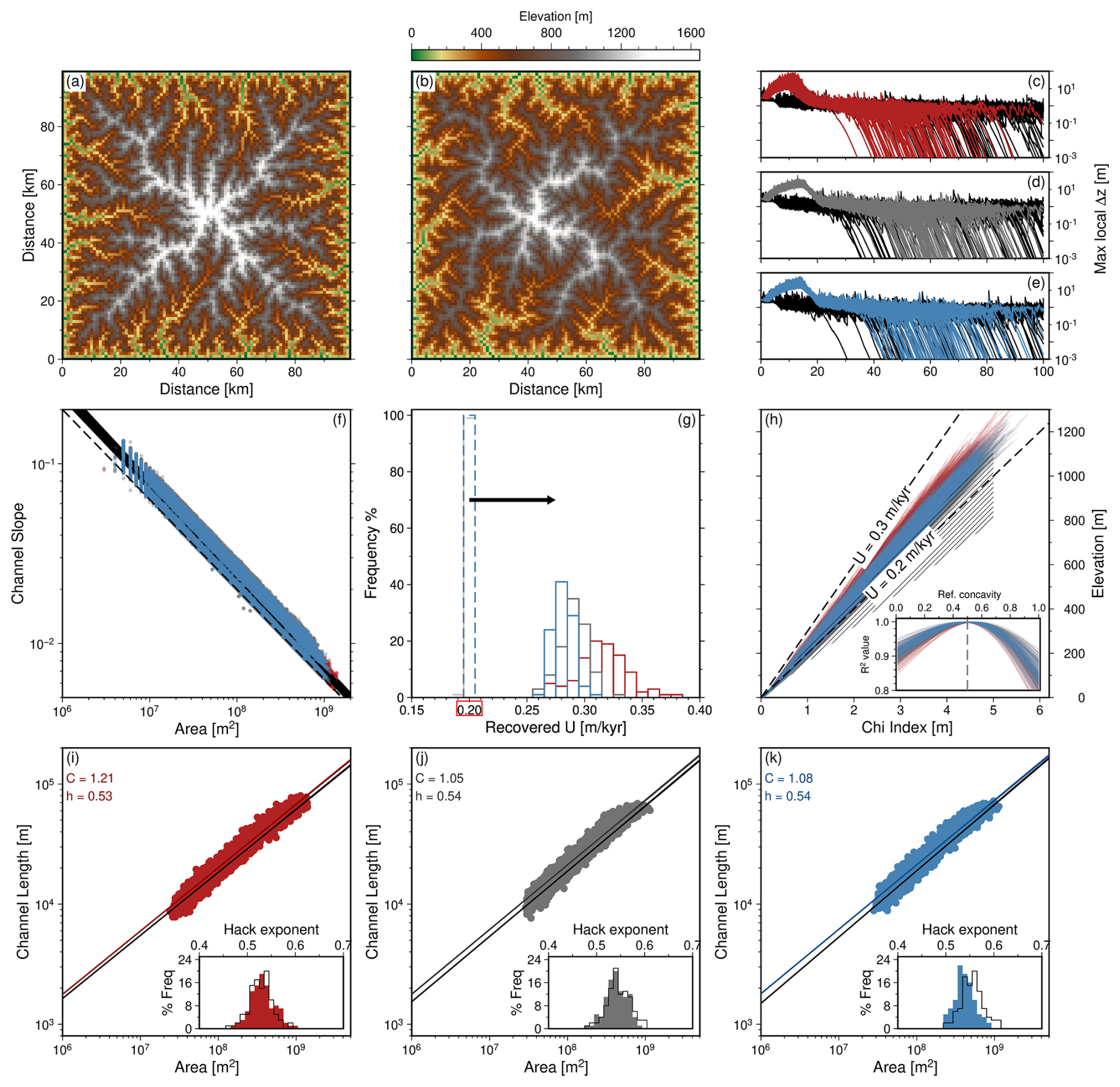
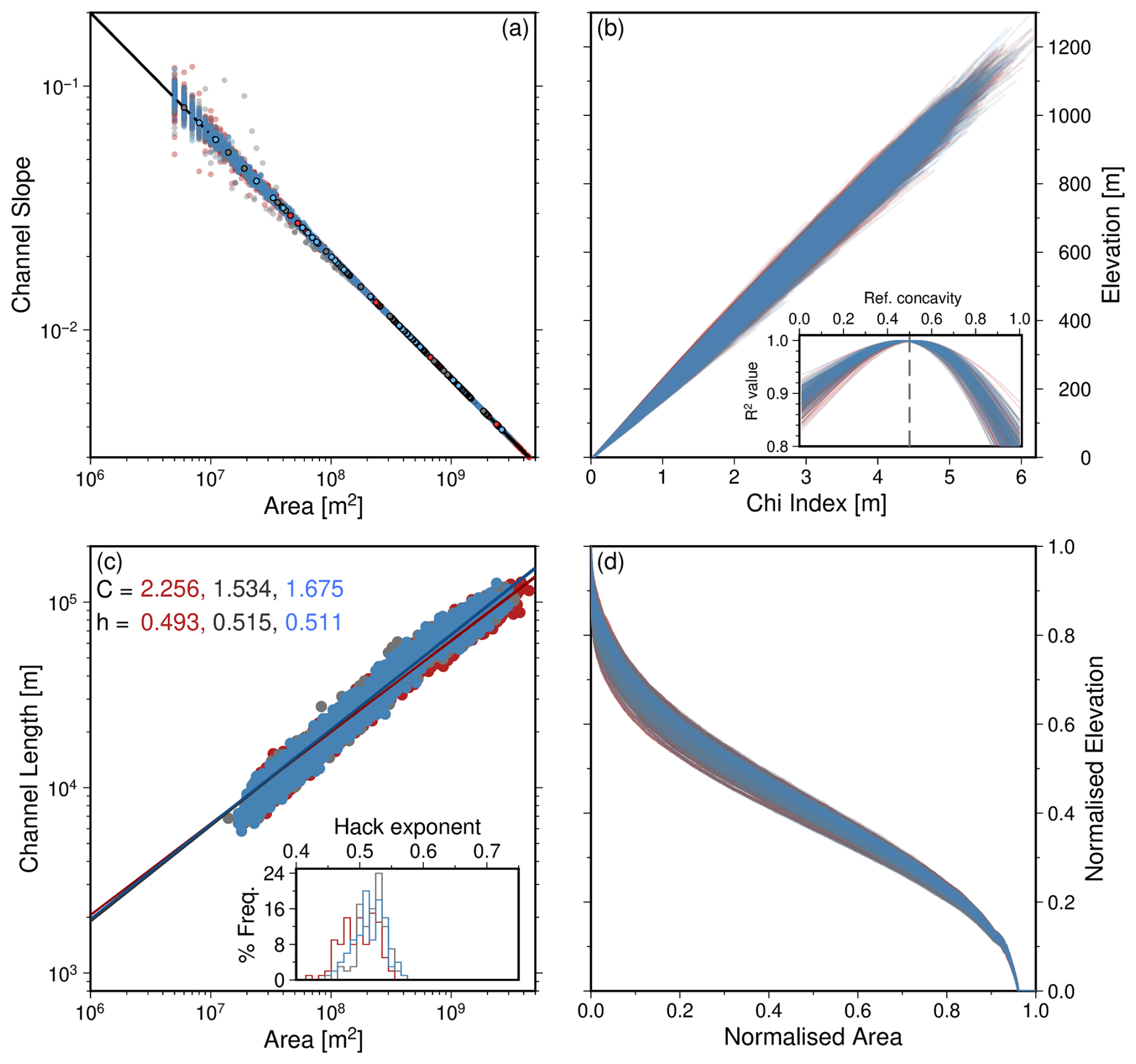
Figure 17 Comparison of geomorphic metrics for steady state “square” landscapes evolving with initial or quenched noise. (a) Topography (at 100 Myr) generated with 0–1 m of identical (i.e., quenched) white noise added at every time step, i.e., scenario B in Fig. 3. (b) Landscape at 100 Myr generated with identical initial condition to (a) but with no additional noise, i.e., scenario A in Fig. 3. (c–e) Changes in maximum local relief in M=100 landscapes generated with only initial noise (black lines), and red, white or blue quenched noise (coloured lines). (f–k) Geomorphic metrics for M=100 red, white or blue landscapes generated with quenched noise unless otherwise indicated. (f) Slope-area relationship for grid nodes with drainage area exceeding 4 km². Black lines = linear regression. (g) Solid lines = histograms of uplift rate recovered from each of the 100 red, white, and blue quenched noise landscapes from slope-area analysis. Dashed lines = results for landscapes with only initial noise. Red rectangle = “true” uplift rate used to parametrise the LEMs. (h) z(χ) profiles for the main channel and its tributaries of the largest drainage basin in each simulation, produced using θ=0.5. Black hashed region shows range of equivalent z(χ) profiles when quenched noise with elevations −0.5 to 0.5 m is added (see Sect. 3.2.2 for details). Inset shows the R² value of different reference concavities. (i–k) Upstream drainage area vs. channel length for main trunks of the forty largest drainage networks in the red (i), white (j), and blue (k) quenched noise landscapes. Black line = non-linear least squares best-fit. Filled/black histograms show the range in Hack exponent for each simulations from quenched noise/initial noise landscapes.

This figure demonstrates that the geometry of the drainage network in a landscape generated with quenched noise can differ from that in a landscape generated with the same arrangement of noise only in its initial condition. Landscapes generated with the same distributions (but different arrangements) of quenched noise tend to have drainage patterns that are more similar to each other than those generated with different arrangements of initial noise (cf. Figs. 3 and S6). We attribute these results to the enhanced role noise plays in determining the location of drainage networks when it is quenched.

Figure 17c–e illustrates that landscapes with quenched noise tend to have an early phase during which they tend to move away from equilibrium (see increasing Δz between 0–15 Myr) before moving towards equilibrium (Δz→0 at T>15 Myr). Such trajectories have not been observed in models in which noise is only inserted into initial conditions (see black curves in Fig. 17c–e).

3.2.2 Slope-area, χ, and length-area analyses

Figure 17f–g show that slope-area data becomes more scattered when noise is quenched compared to when it is only inserted into initial conditions. A consequence of this scatter is that there is more variability in the lines of best fit (shown in Fig. 17f), including their slopes and intercepts. Consequently, recovery of the true uplift rate becomes more unreliable, even when elevation added by quenched noise is corrected (average: 0.05 m kyr⁻¹; see arrow in Fig. 17g), or when quenched noise has a mean elevation of 0 m (Fig. S9g). Recovered rates are 25 % to 85 % higher than the true value of 0.2 m kyr⁻¹. Uplift rates recovered from landscapes with quenched red noise have greater variance than those generated with quenched white or blue noise. We explore why distributions of recovered values of U are not centred at 0.25 m kyr⁻¹ in the Discussion section.

To test the impact of quenched noise on uplift rates extracted from χ analyses we examine the consequences of fixing θ to its true value (0.5; Eq. 20). Figure 17h shows that z(χ) profiles generated in this way are linear with some scatter. Landscapes with quenched red noise tend to have higher elevations as a function of χ than those with quenched white or blue noise. We note that, in contrast, noise inserted only into initial conditions results in more similarly distributed z(χ) profiles (ensembles 1, 4, 7; cf. Figs. 12b and 17h). The best-fitting concavity values are centred on the true value of 0.5 in both cases (see inset panels in Figs. 12b and 17h). The black hashed region in Fig. 17h shows that scatter in z(χ) profiles is also present when quenched noise has elevations of −0.5 to 0.5 m (and mean elevation of 0).

Figure 17i–k illustrates that there can be large variability in Hack exponent, h, values when noise is quenched. The distributions of h are broadly similar in simulations with quenched noise and noise inserted only into the starting condition (cf. coloured and black histograms in Fig. 17i–k).

3.3 Scenario C: spatio-temporal noise

There are two main differences in the results obtained from landscapes generated with quenched or spatio-temporal noise. The first unsurprising result is that landscapes with spatio-temporal noise never reach true steady state (Fig. 18c). Time series of maximum local Δz show that, similar to models in scenario B, simulations with spatio-temporal noise take up to 20 Myr to stabilise around a gradually decreasing mean value. However, they do not reach true numerical steady state (i.e., Δz=0) as a result of the arrangements of added noise changing at each time step. The absence of spatial consistency in added noise can prevent erosion from balancing the added elevations within a single time step. The second main difference is that, unlike quenched noise, adding spatio-temporal noise produces less scattered slope-area relationships (Fig. 18f). Consequently, uplift rates recovered via linear regression are more tightly clustered than those generated in scenario B. However, they are offset from the true value by the added noise (see arrow in Fig. 18g). This offset is not present when spatio-temporal noise has a mean elevation of 0 m (Fig. S10g). A corollary is that recovering true tectonic uplift rates requires information about the amplitude and distribution of noise in a landscape. In contrast, the results from z(χ) analyses, drainage probabilities, and channel length-area relationships are all broadly similar to those obtained for scenario B (Figs. 18h, i–k, and S6g–i).

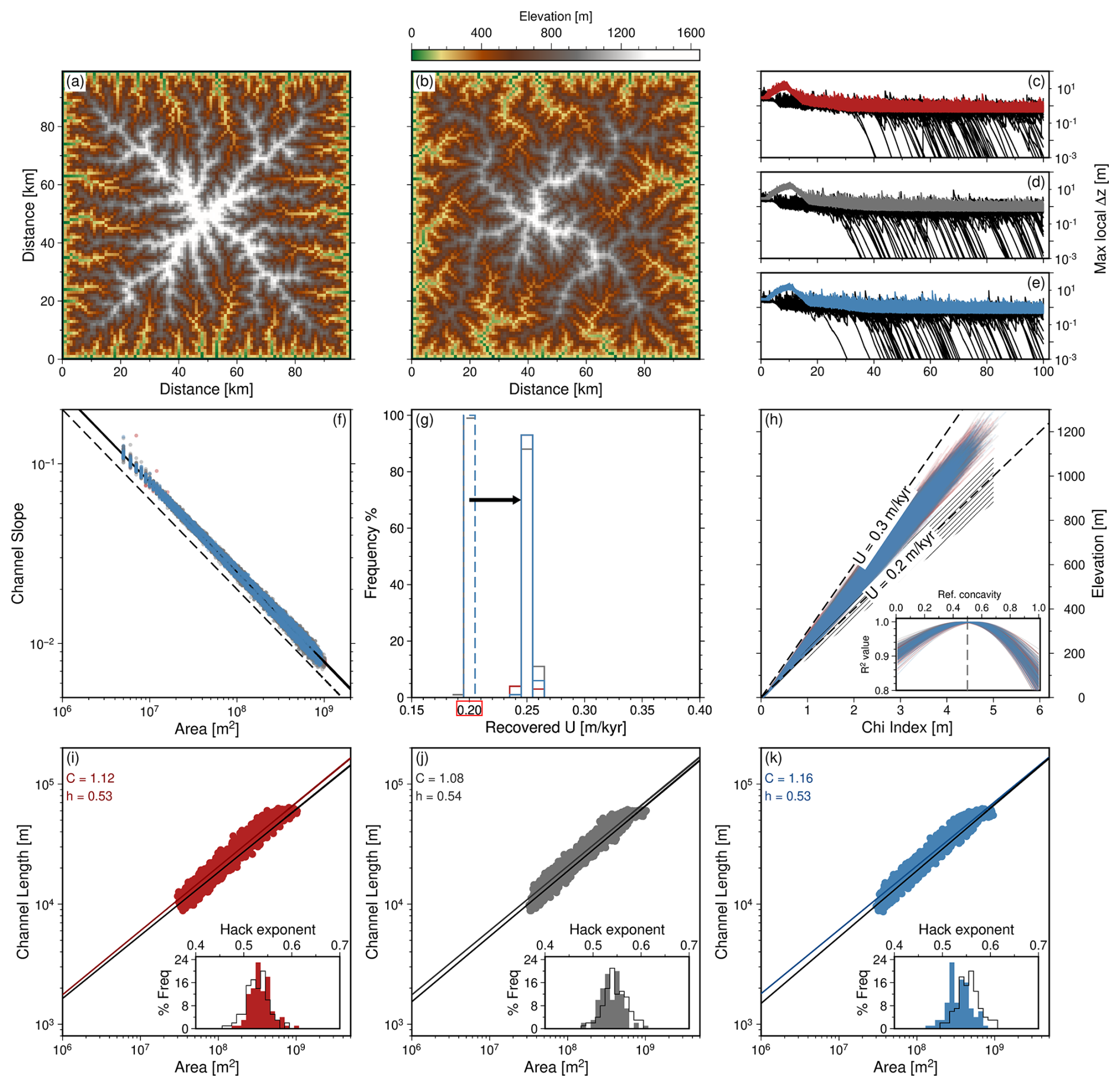
Figure 18 Comparison of geomorphic metrics for “steady state” “square” landscapes evolving with initial or spatio-temporal noise. (a) Example of a “steady state” landscape (at 100 Myr) generated with different (spatio-temporal) arrangements of white noise added at each time step. (b) “Steady state” landscape (at 100 Myr) generated with identical initial condition to (a). (c–k) Same annotation as for Fig. 17 for models with spatio-temporal red, white or blue noise, or noise added only to the initial condition.

3.4 Scenario D: addition of un-eroded noise

The impact on geomorphic metrics of adding noise to a steady state landscape such that the noise remains un-eroded is shown in Figs. 19 and 20. Adding noise in this way acts to “blur” topography, and increases the proportion of elevations which are between 20 %–50 % of the maximum height, shown in Fig. 19c. Whilst the impact of adding 0–20 m of noise is subtle on the longitudinal profiles shown in Fig. 19d, this noise generates scatter in the slope-area data such that recovered uplift rates are 50 % larger than the steady state case. z(χ) profiles are less affected by 0–20 m of un-eroded noise, but become highly scattered when 0–200 m of un-eroded noise is added to the landscape. Slope-area analysis is demonstrably an inappropriate technique to use for recovering U and θ from steady state landscapes containing, say, 200 m of un-eroded noise. In fact, even 20 m of added noise can result in calculated uplift rates being unreliable (Figs. 20b, S11–S13).

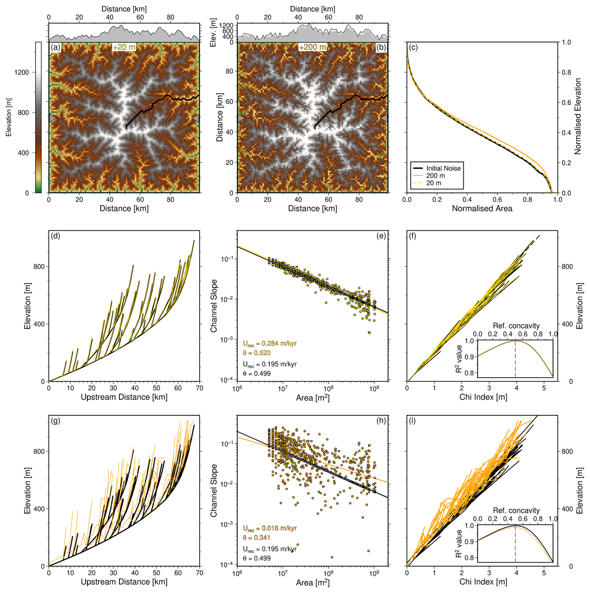
Figure 19 Impact of un-eroded noise on metrics: An example. (a) Steady state “square” landscape generated with up to 1 m of white noise in its initial condition (Fig. 4: ensemble 1), and with up to 20 m of white noise added after the final model time step. Filled grey transect shows topographic profile of steady state landscape (without final noise). (b) Same landscape as in panel (a), but with up to 200 m of un-eroded noise. Black outline shows location of the same (longest) river in landscapes with final noise added. (c–i) Yellow/orange = geometries and metrics extracted from landscapes with up to 20 and 200 m of un-eroded noise. (c) Black dashed curve = hypsometry of landscape shown in panel (a); colours = hypsometries of landscapes with un-eroded noise. (d–f) Longitudinal profiles of rivers in largest drainage basin (see panel (a)), slope-area and χ analyses of rivers shown in panel (d) respectively, for steady state landscape and landscape with 0–20 m noise added. (g–i) As above, for landscape with 0–200 m noise added. Metrics for un-eroded red and blue noise are shown in Figs. S12 and S13.

4 Discussion

4.1 Distributions of geomorphic metrics and determinism

We synthesise the results obtained from scenarios A–D in Fig. 20 and use this as a framework to discuss key findings regarding geomorphic metrics.

Across almost all scenarios we obtain distributions of results from model ensembles. In other words, slope-area relationships, χ analysis, and length-area relationships are sensitive to noise inserted into the models. These results emphasise the benefits of using model ensembles or probabilistic approaches to landscape evolution modelling (rather than relying on interpretation of singular, or small-batch, runs of stream power-based models). An ensemble-based approach permits characterisation of, for instance, uncertainty and dependence on noisy (starting) conditions, model assumptions or model parameter values. These results clearly indicate that caution is required to avoid over-interpretation of results from single models (and the real world) which may be outliers with geometries that depend on an arbitrary noisy starting condition, which in reality represents (largely) unknowable palaeo-conditions (topography, weather, climate, biota, etc.) It emphasises the importance of embracing the fundamental unknowability inherent to landscapes and thus the importance of quantifying the impact of noise (and especially its distributions) on geometric predictions (e.g., of topography, sedimentary flux) and calculated metrics (see e.g., Perron and Fagherazzi, 2012; Gray et al., 2017; Lyons et al., 2020; Roberts and Wani, 2024; Thompson Jobe and Reitman, 2025).

4.1.1 Uplift rates and concavity indices recovered from slope-area and χ analyses

The sensitivity of slope data to added noise has previously been discussed, for example in Roberts et al. (2012b) and Mudd et al. (2018). In this study, we show that, when operating in a numerical steady state under spatially invariant uplift, slope-area analysis can be used to recover input values of erosional parameters and uplift rates (see e.g., Figs. 11, 20a–b). However, we also show that this technique does not yield accurate results under conditions of spatially variable uplift (Fig. 15), or when noise is added during or at the end of a simulation (Figs. 19, 20a–b). This finding is also true of χ analysis, which is impacted by noise in a different way.

The specific arrangement and distribution of noise used as a starting condition can change the value of the reference concavity which best linearises z(χ) profiles. The sensitivity of χ to reference concavity values has also been shown by Gailleton et al. (2021). Best-fitting reference concavity values are shown in Fig. 20c, and can vary from the true value of 0.5 (in this study). The colour of noise has a minor impact on the variance of the distributions. The distributions become less centred on 0.5 when the amplitude of initial or final noise increases, or when quenched noise is present. Figure 14 shows the impact of using different values of θ_ref to generate z(χ) plots, and the resulting distributions of uplift rate calculated from the slopes of these profile are shown in Fig. 20e. Several clusters of distributions exist because of the different best-fitting values of θ_ref, with calculated uplift rates varying between 0.5 and 1.5× the true uplift rate for scenario A, and up to 2× the true uplift rate for scenarios B–D. Even in the case of z(χ) profiles calculated using the true value of θ=0.5, rather than the best-fitting θ, recovered uplift rates are distributed around the true uplift rate of 0.2 m kyr⁻¹ (Fig. 20d). This result highlights the uncertainties generated from noisy conditions in landscape evolution models and thus the challenges associated with interpreting outputs from single models.

A further complication in recovering tectonic information from slope-area and z(χ) analyses arises in cases where uplift is spatially variable, e.g., for domal landscapes. In general, Fig. 15a–b demonstrate that slope-area analysis is an inappropriate tool for recovering uplift rates and erosional parameter values from domal landscapes, or more broadly landscapes with spatially variable uplift. We extend this comment to also encompass χ analysis when used in this way, given the absence of (col)linearity of z(χ) profiles in Fig. 15b and the best-fitting reference concavity being close to 1, rather than the true value of 0.5. We acknowledge that modifications to χ analysis exist to account for spatially variable uplift (see e.g., Mudd et al., 2014; Hergarten et al., 2016; Mudd et al., 2018). In practice, both slope-area analysis and χ analysis rely on an assumption of steady state, which we discuss in Sect. 4.2. Our result, generated under steady state conditions and different arrangements, distributions, or implementations of noise extend those of Mudd et al. (2018), who generate examples of transient synthetic landscapes with spatially variable erodibility or uplift rate, and calculate distributions of best-fitting reference concavities from different basins, across a range of calculation methods.

One could also argue that the uplift applied to the “square” landscapes in scenario B is spatially variable, due to the presence of quenched noise. A consequence of quenched noise is to add scatter to slope-area data such that recovered uplift rates are distributed between 0.26 and 0.37 m kyr⁻¹ (Figs. 17g, 20b). Given that the mean elevation of noise added per time step is 0.5 m, and the maximum elevation added is 1 m, it might be expected that quenched noise contributes an additional mean and maximum uplift rate of 0.05 and 0.1 m kyr⁻¹, leading to mean and maximum calculated uplift rates of 0.25 and 0.3 m kyr⁻¹ respectively. We interpret recovered uplift rates being up to 0.37 m kyr⁻¹ as the result of scattered data and trade-offs between the slope and intercept (from which uplift rates are calculated) of the best-fitting linear regression. The presence of quenched noise in models tends to generate considerable spread in slope-area data, and thus in calculated intercepts (and thus uplift rates). In contrast, uplift rates recovered from slope-area data in scenario C are offset from the true uplift rate by 0.05 m kyr⁻¹, i.e., the mean amplitude of uplift added from noise. We note that it is unlikely that the true amplitudes of noise are known for real landscapes, meaning that it is not trivial and perhaps impossible in some circumstances to correct uplift rates calculated in this way for noise.

4.1.2 Variability in Hack exponent value

A consistent result across all model scenarios and ensembles is the variability in Hack exponent value, h, due to different arrangements and distributions of noise. Hack exponent values vary between 0.45 and 0.75, generally a larger range than previous studies which calculate h based on data from natural landscapes across regional and global scales (Hack, 1957; Mueller, 1972; Montgomery and Dietrich, 1992; O'Malley, 2020; He et al., 2024; Singer et al., 2024). Many of these studies find 0.45 $\le h\le \mathrm{0.7}$, whilst dimensional analysis predicts h=0.5. It has been suggested that Hack exponent values < 0.5 imply that drainage basins are widening and values > 0.5 imply elongating basins (Mueller, 1972). Many of the distributions of h that we calculate from our models have values > 0.5, indicating that, if we accept this reasoning, basins are elongating more than they are widening. Figure 20f demonstrates that on average, landscapes initialised with red noise in Scenarios A–D produce lower Hack exponent values than their white and blue noise counterparts, implying that their catchments are elongating at a slower rate. However, it is unclear that the temporal evolution of drainage basins can be related to length-area relationships obtained at a single model time step, and in many cases the topography is at a numerical steady state (i.e., $\partial z/\partial t=\mathrm{0}$ everywhere), indicating no change in basin geometry. Prior studies have recognised the potential for drainage basin scale to influence the calculation of h (Mandelbrot and Wheeler, 1983; Robert and Roy, 1990). The drainage basins in our models used to calculate Hack exponents range in size from 10⁷–10⁹ m². These sizes fall within the range of basin areas from which Hack exponents have been calculated in previous studies, though are closer in size to those originally examined by Hack (1957), who found h>0.5. Extraction of channel lengths and upstream areas from synthetic landscapes also circumvents measurement errors encountered when calculating these metrics from field data or digital elevation models.

Climatic conditions have also been suggested to influence Hack exponent values. For example, Yi et al. (2018) categorise drainage basins in the contiguous United States by aridity index and find that h≃0.49 for basins in arid regions, and h≃0.59 for basins in humid regions. Conversely, Singer et al. (2024) find from a global drainage dataset that h increases with increasing aridity. Our findings suggest that different arrangements and distributions of noise within landscape evolution models produce at least as much variance in Hack exponent values as climatic variables. This result is similar to that of Sassolas-Serrayet et al. (2018) and O'Malley (2020), who found a limited influence of (modern day) mean annual precipitation (and lithology) on Hack exponent values calculated from observational data.

4.2 An assumption of steady state

A fundamental assumption underlying the recovery of uplift rates and erosional parameter values from widely used techniques such as slope-area or χ analyses is that uplift rates are balanced by erosion, i.e., there exists a topographic steady state. When operating with synthetic landscapes it is straightforward to numerically verify that this condition is true (e.g., Fig. 5). Our results demonstrate that, even under conditions of steady state, recovery of uplift rates and erosional information is complicated by the choice of how noise is included within models, which leads to distributions of recovered values, shown in Fig. 20.

Notwithstanding inconsistencies in how steady state topography is defined, as outlined by Gasparini et al. (2024), in general, observational evidence to confirm that landscapes in the real-world are at topographic steady state is scant. In fact, most continental topography appears to refute the steady state assumption, which in general must be wrong because geological observations (e.g., uplifted marine rock; sedimentary isopachs indicating punctuated sedimentary flux; incision rates from radiometrically dated rocks) demonstrate that topography increases and decreases in elevation on a variety of spatial and temporal scales, and may horizontally advect (e.g., Rust and Summerfield, 1990; Young and McDougall, 1993; Roberts and Kirschbaum, 1995; Willett and Brandon, 2002; Karlstrom et al., 2007; Stephenson et al., 2019; Racano et al., 2020; Malatesta et al., 2022). These observations, alongside the findings from our synthetic landscapes, and results from some analogue models, call into question the utility of geomorphic techniques which rely on assumptions of steady state (see e.g., Hasbargen and Paola, 2000).

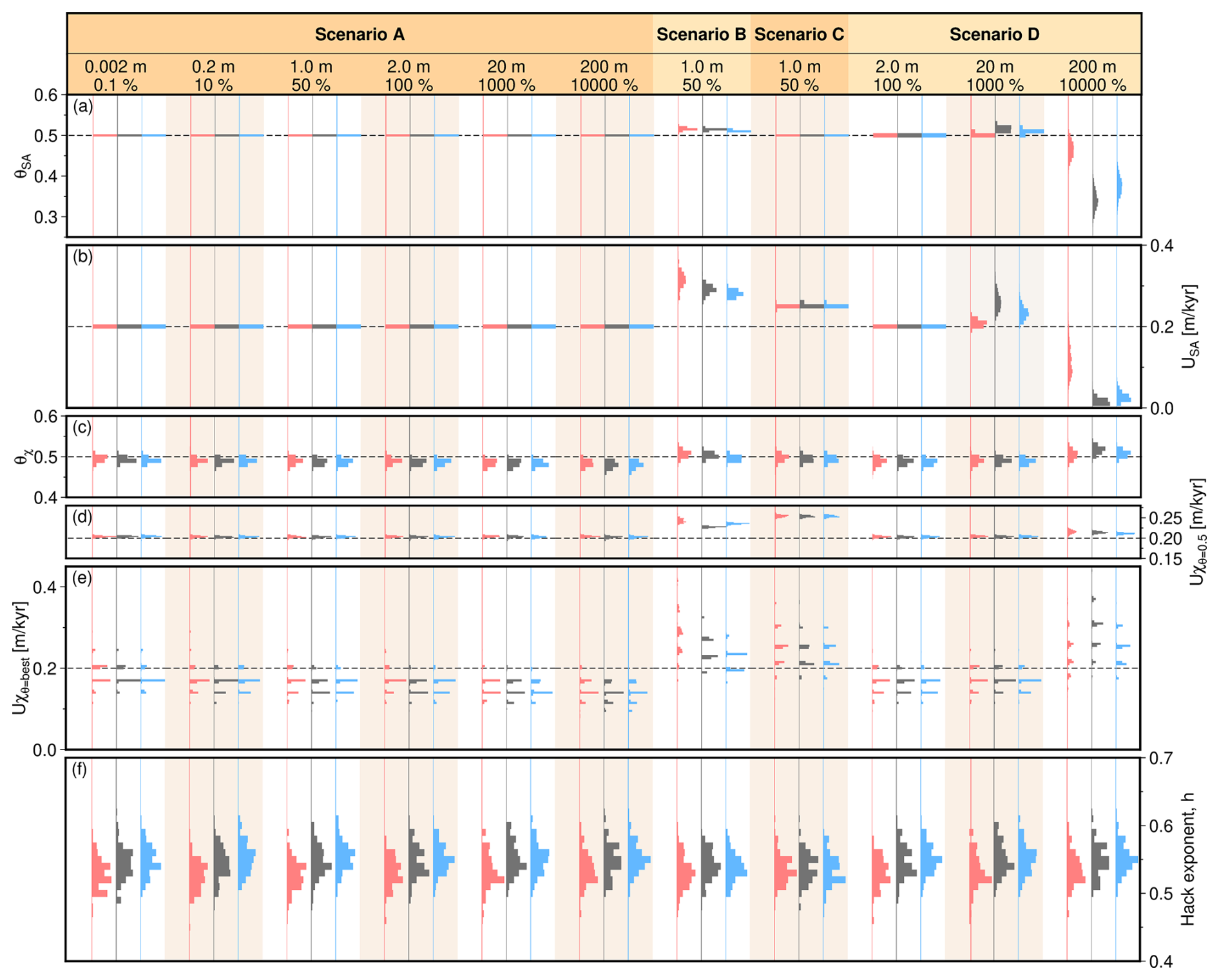
Figure 20 Impact of noise on variance of geomorphic metrics from steady state landscapes. Series of histograms showing the distribution of different geomorphic metrics under different noisy conditions for the “square” landscape (Scenarios A–D; see Figs. 3–4). Black dashed lines = true values, used to produce the LEMs. For the quenched and spatio-temporal examples, up to 1 m of noise was added at every time step. (a–b) Concavity index and uplift rate recovered from slope-area analysis. (c) Value of concavity index that best linearises χ-elevation plots. (d) Corresponding uplift rate associated with the slope of the best-fitting line of χ-elevation data, from the rivers of the four largest basins transformed using θ=0.5. (e) As per (d), for a slope of the best-fitting line of χ-elevation data from the rivers of the four largest basins, transformed using the respective best-fitting values of θ. (f) Values of Hack exponent calculated from river length-upstream area relationships.

4.3 Drainage planform variability and maximum drainage sizes

Figures 7 and 9 demonstrate how different arrangements and colours of noise can lead to different drainage planform structures. This result extends that of Kwang and Parker (2019), who interpret the lasting influence of initial conditions in landscape evolution models as an absence of other mechanisms that can remove initial network structure (e.g., lateral erosion and migration of channels present in natural environments; Kwang et al., 2021). Figure 7 emphasises how landscapes that evolve with identical tectonic histories can have different geometries due to noise. It is clear that in such cases using Euclidean-based approaches to compare modelled and observed elevations of entire landscapes may lead to undesirable high misfit when tectonic histories are in fact similar. Instead, minimising misfits (via inverse modelling for instance) to recover tectonic (uplift) rates probably requires techniques that can “see through” the local complexity of precise planform arrangements introduced by specific arrangements of noise (e.g., Morris et al., 2023). More generally, broadly equal probabilities of channel locations under the uplift and erosional conditions modelled (Fig. 9) indicates that caution should be taken when interpreting drainage planform structures, or related metrics, from single models, or observations. We note that the drainage planform patterns of “square” landscapes containing quenched or spatio-temporal noise (scenarios B, C) more closely resemble the general structure of probabilistic drainage maps than landscapes containing only initial noise (scenario A). For instance, landscapes generated with spatio-temporal or quenched noise tend to have interfluves and high topography with low drainage probability extending in a “cross” from the centre of the domain to each corner; cf. Figs. 17a–b, 18a–b, S6. Perhaps surprisingly, even landscapes with quenched noise display this pattern. These results indicate that repeated insertion of noise (i.e. at each time step), reduces the influence of noisy initial conditions on the geometries of landscapes at large scales.

Similarly, the position of drainage divides can also depend on noisy starting conditions, for example the areas of low probability in the “escarpment” landscapes shown in Fig. 9d–f. In particular, models initialised with red noise have less well-defined regions of low drainage probability. We interpret this result as a consequence of long wavelength changes in topography permitting initial flow-lines to span across more than half of the domain, even after sink-filling. Conversely, the shorter wavelength topographic roughness present in landscapes initialised with white or blue noise means that the largest drainage basins usually terminate at the centre of the domain, leading to consistent regions of low drainage probability (see Fig. 9b–c). We also interpret this as a mechanism for why the largest drainage basins in “square” landscapes initialised with red noise are, on average, larger than those from landscapes initialised with white or blue noise (Fig. 8).

4.4 Comparison to natural landscapes

4.4.1 The relevance of initial, quenched, and spatio-temporal noise

The result that distributions in geomorphic metrics arise from different arrangements, colours, and implementations of noise within landscape evolution models is a finding similar to that of Perron and Fagherazzi (2012), and emphasises that the application of noise is not an arbitrary model choice. Whilst noisy initial topography enables the generation of realistic drainage planforms within models, it can also be representative of natural processes or features. For example, noisy starting conditions may be considered to represent a palaeotopography. In some studies, it may be inappropriate to solely implement random noise as a starting condition, for example where it may be possible to guess palaeotopography prior to volcanic eruption or ice cover, for instance (e.g., Paxman et al., 2019; Barnhart et al., 2020b; O'Hara et al., 2024). Yet in many other studies and at different scales, palaeotopography is unknowable and therefore assessing uncertainties using ensembles of models with variable starting conditions is probably a sensible, perhaps necessary, strategy.

However, it is questionable whether the application of noise exclusively as an initial condition is a reasonable assumption. Perhaps incorporating noise throughout model run time is closer to reality. For instance, erosion of substrate with constant (in time) erodibilities, or landsliding occurring repeatedly in the same place, could be regarded as sources of quenched (i.e., fixed for all time) noise. In general however, geomorphic noise in natural landscapes must vary as a function of space and time. For instance, as lithologies with different erodibilities are exposed. Thus, in scenarios B–C we explore the consequences of adding quenched and spatio-temporal red, white, or blue noise with amplitudes 0 to 1 m and −0.5 to 0.5 m throughout model run time. Figures 17g and 18g show that noise generates uncertainty in recovered uplift rates, which can be considerable (see also Figs. S9 and S10).

4.4.2 Colour, scale, and metrics

The spectral content of synthetic steady state landscapes generated in scenario A is characteristic of red noise ($\mathit{\varphi }\propto k^{-\mathrm{2}}$). Similar spectral characteristics have been identified in natural landscapes, across scales from centimetres to thousands of kilometres (e.g., Balmino, 1993; Birnir et al., 2001; Perron et al., 2008; Booth et al., 2009; Roberts et al., 2019). Wavelet spectral analysis of longitudinal profiles for large African rivers shows that their power spectra can be characterised as pink noise ($\mathit{\varphi }\propto k^{-\mathrm{1}}$) at wavelengths ≲ 100 km and as red noise ($\mathit{\varphi }\propto k^{-\mathrm{2}}$) at longer wavelengths (Roberts et al., 2019). The transition from complexity at local scales to relative predictability at large scales emphasises why some geomorphic metrics are more sensitive to noise than others. For example, it is unsurprising that the recovery of uplift rates or erosional parameter values from derivatives (i.e., topographic slopes, $\mathrm{d}z/\mathrm{d}x$, or gradients of z(χ) profiles, $\mathrm{d}z/\mathrm{d}\mathit{\chi }$) is hampered by the addition of noise; Fig. 19. In these examples, metrics which incorporate topographic information from restricted spatial scales are likely to have lower signal to noise ratios, and differentiation of noisy data accentuates uncertainties. In comparison, geomorphic metrics which consider the entire shapes of landscapes, such as hypsometry, appear less sensitive to noise.

4.5 Limitations and recommendations

Obvious ways in which the work presented could be extended include assessing the impact of noise using other landscape modelling software packages (e.g., Badlands, CHILD, FastScape) or by randomising flow directions (Tucker et al., 2001; Salles, 2016; Salles and Hardiman, 2016; Bovy, 2021). Secondly, we note that alternative approaches to defining noise could be examined. We briefly explored the use of simplex noise (related to Perlin noise) but found it to generate linear artefacts (Perlin, 2002). Third, there are a host of additional geomorphic properties that we have not examined that may be impacted by noise, e.g., sedimentary flux.

Our first recommendation concerns the application of noise within landscape evolution models. Noise should be expected to always be present, even if it is difficult to quantify, in real landscapes (Birnir et al., 2001). We therefore consider the application of noise as an important, and not arbitrary, choice within models that seek to represent natural landscapes and underlying mechanisms which govern their evolution. We have shown that two widely used techniques (namely slope-area and χ analyses) for recovering uplift rates or erosional parameter values from topography can give results that are wrong but look correct, even when a landscape is demonstrably at topographic steady state. If such methodologies are used, our suggestions are to, first, do more, for instance re-run models many times to test the impact of uncertainties (noise), and to explicitly communicate the distributions (colours) and amplitudes of noise used. Second, do it better, i.e., find ways to ensure that fundamental assumptions, such as topographic steady state, are appropriate. One pragmatic way of doing so is to use independent evidence (e.g., geologic evidence of uplift or erosion) to test results. Third, above all else, acknowledge and communicate uncertainties, e.g., in calculated uplift rates or concavity indices from metrics-based approaches.

Our second recommendation is to use or develop other methodologies that allow assumptions about topographic steady state to be relaxed, and explicitly incorporate uncertainties. Inverse modelling of landscapes for uplift rate histories, for instance, allows one to avoid many of the pitfalls associated with metrics-based approaches, in particular when probabilistic approaches are taken (e.g., Willgoose et al., 2003; Croissant and Braun, 2014; Rudge et al., 2015).

5 Conclusions

Landscapes with the same uplift and erosional forcings evolved to equilibrium conditions using the SPM can have very variable geometries as a result of noise inserted into their starting conditions or as models evolve. Extraction of geomorphic information from such landscapes using common metrics-based approaches (slope-area, χ), and subsequent recovery of uplift rates, erosional parameters values, and Hack exponents, show that varying the arrangement, distribution, and implementation of even small amplitudes (<1 % of cumulative uplift) of noise can produce results with broad distributions. Adding quenched noise to models produces more uncertainty in recovered uplift rates than when noise varies spatio-temporally. Observations of the spectral content in natural landscapes indicates that features with red noise are prevalent. The largest drainage basins produced in modelled landscapes initialised with red noise tend to be larger than those in landscapes initialised with white or blue noise. Positions of drainage divides in landscapes initialised with red noise are less predictable than those generated with white or blue noise. All introduce considerable uncertainties in the position of drainage divides and basin geometries. The production of distributions in results arising from noisy conditions illustrates the benefits of probabilistic or ensemble approaches to modelling, and the peril of interpreting predictions from single models. We suggest that assessing the impact of noise on SPM predictions benefits from two considerations. First, utilising ensembles of models. Secondly, assessment of the distributions of geometries including elevations, planforms, drainage divides, length-area relationships, and metrics, e.g., concavity and steepness indices. Doing so provides insight into the uncertainties that arise solely through the incorporation of noise, which can be considerable.