Influence of network geometry on long-term morphodynamics of alluvial rivers

Alluvial rivers respond to external forcings such as variations in sediment supply, water supply and base level by aggrading, incising and adjusting the rates at which they transport sediment. These processes are recorded by landforms, such as terraces and fans, that develop along river courses, and by stratigraphy in downstream sedimentary basins. Many concepts we use to interpret such records are derived from models that treat alluvial rivers as single-segment streams: for example, the length of an alluvial river has been shown to set its response time to external forcing. However, alluvial rivers in nature exist within interconnected networks, complicating the application of such concepts to real systems. We therefore adapted a model describing long-profile evolution and sediment transport by transport-limited, gravel-bed alluvial rivers to account for network structure, and explored the response of large numbers of synthetic networks to sinusoidally varying sediment and water supply. We show that, in some respects, networks behave similarly to single-segment models. In particular, single-segment models predict well properties that integrate across the entire network, such as the total sediment output. We use this behaviour to define an empirical network response time, and show that this response time scales with network mean length, or the mean distance from all a network's inlets to its outlet. Nevertheless, interactions between segments do lead to complex signal propagation within networks: amplitudes and timings of aggradation and incision vary between minor tributaries and major trunk streams, and between upstream and downstream parts of the network, in ways that depend on each individual network's structure. We conclude that, while single-segment models may be useful for some applications, detailed studies of specific catchments require a modelling framework that accounts for their specific network structure.

1 Introduction

Alluvial river networks are fundamental features of Earth's surface, controlling the movement of water and sediment through the landscape. They host fluvial landforms, such as terraces and fans, and deliver sediment to downstream sedimentary basins. The formation of such landforms, the shapes of network longitudinal profiles, and variation in sedimentary facies or accumulation rates in stratigraphic records are commonly attributed to tectonic or environmental change (i.e., external or allogenic forcing; Blum and Törnqvist, 2000; Strasser et al., 2006; Densmore et al., 2007; Bridgland and Westaway, 2008; Wegmann and Pazzaglia, 2009). A major goal for geomorphologists and stratigraphers is, in turn, to infer the timing and magnitude of past tectonic and environmental change from the age and extent of terrace surfaces, as well as the timing and amplitude of stratigraphic fluctuations (e.g., Allen, 2008a; Duller et al., 2010; Macklin et al., 2012; Zhang et al., 2020). Doing so accurately requires an understanding of how alluvial rivers respond to changes in water supply, sediment supply and base level by aggrading, incising and adjusting their sediment-transport rates (Armitage et al., 2011; Romans et al., 2016; Tofelde et al., 2021). Here, we focus on how this response is influenced by the arrangement of alluvial rivers in networks (Fig. 1).

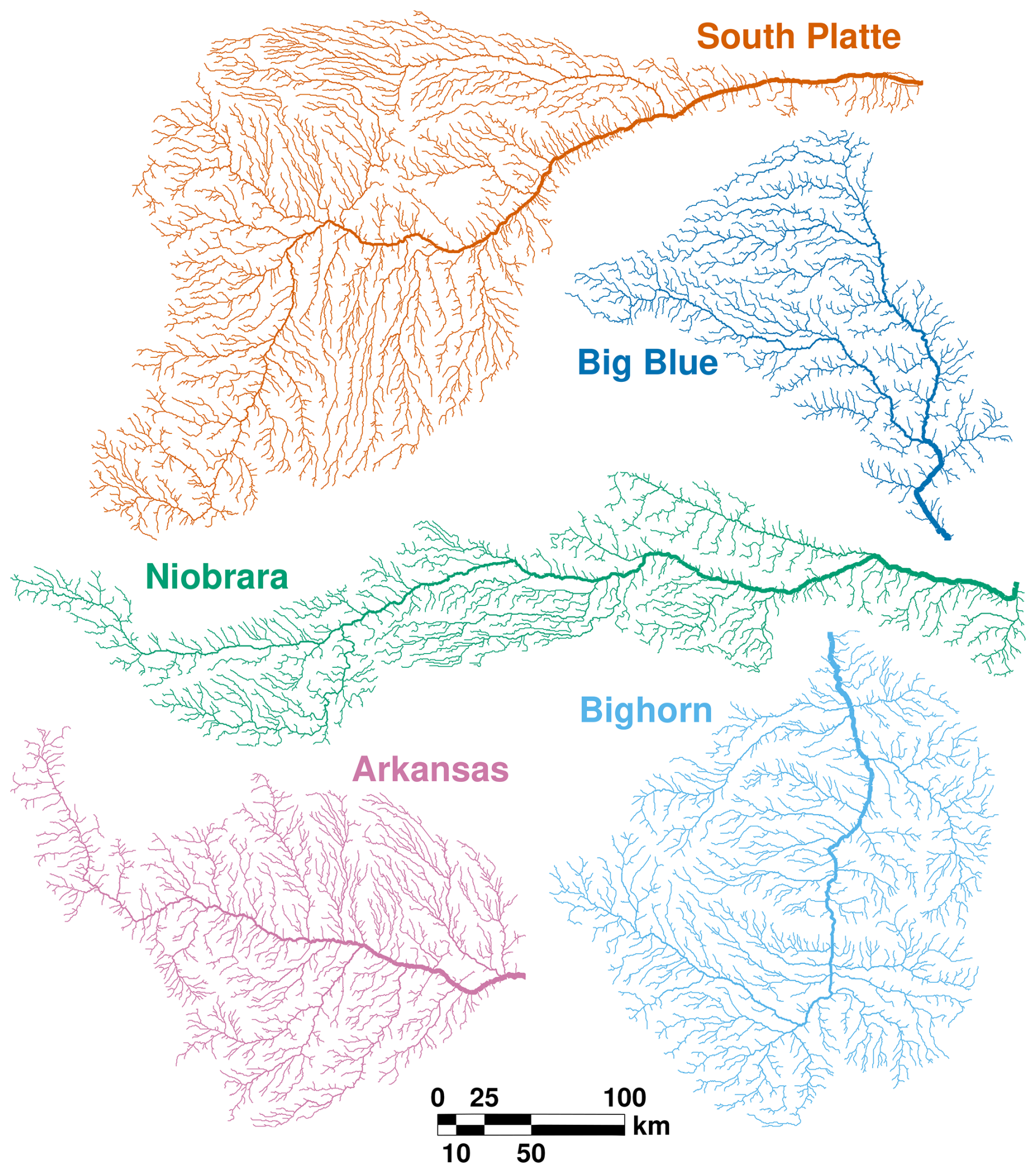
Figure 1 Example catchment planforms from the Great Plains, USA, showing diverse network structures: South Platte (orange), Big Blue (dark blue), Niobrara (green), upper Arkansas (pink) and upper Bighorn (light blue). Scale bar applies to all catchments. Line thickness scales with drainage area. Stream data from the HydroRIVERS database (Lehner and Grill, 2013).

Several lines of evidence suggest that processes of aggradation, incision and sediment transport are intimately connected to the fluvial network structures on which they occur (Benda et al., 2004). At tributary junctions, contrasts in ratios of sediment to water discharge in adjoining streams lead to slope breaks in longitudinal river profiles (Lauer et al., 2008). When steep tributaries with high sediment loads meet gentler trunk streams, fans can develop (Fig. 2a). Such fans can deflect or block the main stream and trigger aggradation along it (Church, 1983; Steffen et al., 2010; Savi et al., 2016, 2020). Alternatively, incision and lateral migration by the main stream can lead to fan abandonment (Larson et al., 2015). Terrace surfaces are often continuous along and between adjoining streams, attesting to the coupled evolution of interconnected river segments (Fig. 2b). Pulses of sediment propagating through river networks can interact and interfere at tributary junctions, leading to “hotspots” of geomorphic change and influencing patterns of sediment export (Benda and Dunne, 1997a; Czuba and Foufoula-Georgiou, 2014, 2015; Roy et al., 2022). Natural river networks present diverse structures (Fig. 1). Furthermore, recent work has highlighted how network structure varies systematically with climatic and tectonic setting, erosional properties, and lithology (e.g., Seybold et al., 2017; Ranjbar et al., 2018; Yi et al., 2018; Getraer and Maloof, 2021; Li et al., 2023; Goren and Shelef, 2024; Pelletier et al., 2025). These results raise the possibility that, if network structure influences alluvial river responses to external forcing, those responses may vary between regions with different climates, rates and styles of tectonic activity, or lithologies (Roy et al., 2022).

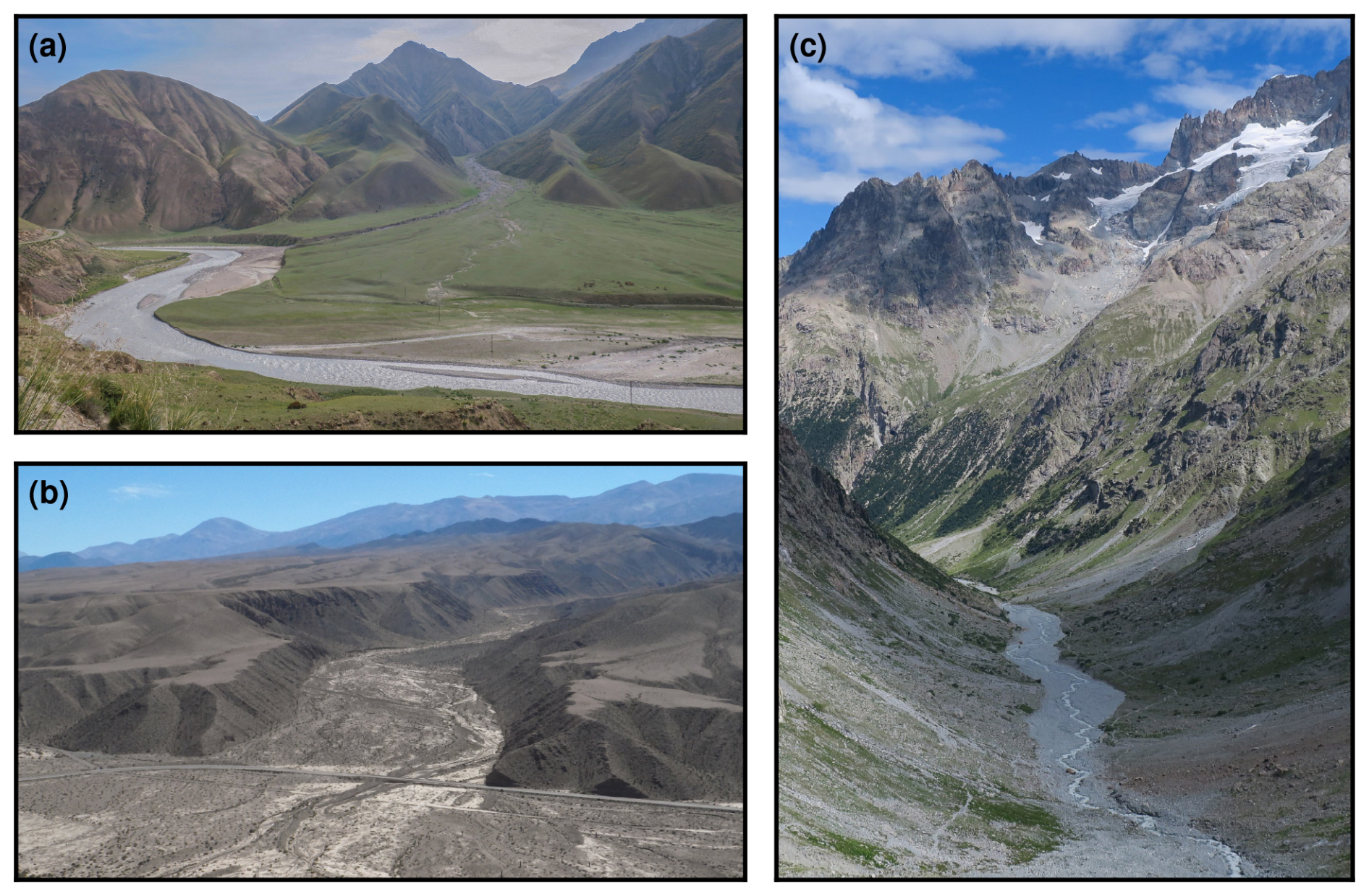
Figure 2 Field photographs of alluvial river landforms associated with network confluences and along-stream supply of sediment. (a) Fan development and interaction with main stream at tributary confluence, Kaindy River (tributary to Saryjaz River), eastern Kyrgyzstan. Photograph by Taylor F. Schildgen. (b) Terraces straddling a main stream–tributary confluence in the Toro basin, near El Alfarcito, NW Argentina. Photograph courtesy of Stefanie Tofelde. (c) Along-stream supply of sediment by debris-covered slopes and debris fans to Vénéon river, Massif des Écrins, France. Photograph by Taylor F. Schildgen.

To quantify relationships between external forcings and alluvial river landforms, longitudinal profiles and stratigraphic archives, a series of conceptual studies have employed numerical models and physical experiments that approximate alluvial river systems as single, one dimensional streams (e.g., Paola et al., 1992; van den Berg van Saparoea and Postma, 2008; Armitage et al., 2011; Simpson and Castelltort, 2012). These models have the advantage of being relatively straightforward to implement and efficient to run, and, despite their simplicity, have led to some useful and influential concepts. Water discharge is either held constant along stream (e.g., Paola et al., 1992; Simpson and Castelltort, 2012; McNab et al., 2023) or set to increase smoothly from inlet to outlet (e.g., Armitage et al., 2011; Goldberg et al., 2021; Braun, 2022). Paola et al. (1992) defined an equilibration time, T_eq, based on a diffusive model of the long-profile evolution of alluvial rivers, which scales with the square of the system length, and showed that the system response to external forcing depends strongly on the frequency of forcing relative to this equilibration time (see also Howard, 1982). Relatedly, it has been argued that stochasticity in sediment transport can lead to degradation (in extreme cases, destruction, or “shredding”) of external signals with timescales similar to or shorter than those of stochastic events (e.g., Jerolmack and Paola, 2010; Griffin et al., 2023). These behaviours are thought to limit what kinds of catchments can record what kinds of signals, whether in terrace sequences or in downstream stratigraphy (Allen, 2008b; Tofelde et al., 2017). Other studies have emphasised how propagation of signals along stream could lead to a lag between the forcing and the river's response, with implications for the interpretation of terrace ages and of stratigraphic time series (Hancock and Anderson, 2002; Braun, 2022; Yuan et al., 2022; McNab et al., 2023).

Concepts derived from single-segment models can, however, be challenging to apply to real systems, either to construct formal tests of model predictions or to facilitate quantitative interpretations of geomorphic and stratigraphic archives. Unlike the single-segment geometries these models consider, the “length” of a river network is poorly defined: channel heads lie at varying distances upstream from network outlets (Fig. 1). Implicit in the arguments of many studies is the idea that timescales of network evolution are controlled by main stream length (e.g., Métivier and Gaudemer, 1999; Castelltort and Van Den Driessche, 2003), but this assumption has not been tested. Furthermore, signal propagation on a network is, conceivably, much more complex than along a single river segment. Along-stream delivery of sediment, which occurs in natural valleys from tributaries as well as from transport down or lateral erosion of adjacent hillslopes, has also generally not been considered (Fig. 2c; Benda and Dunne, 1997b; Benda et al., 2003; Tofelde et al., 2022).

Some modelling studies have begun partly to address the issue of alluvial network responses to external change. Savi et al. (2020) explored interactions between a tributary and main stream in an experimental setting, emphasising that a tributary's influence extends both upstream and downstream of a confluence (see also Benda et al., 2003). Pizzuto (1992) predicted long profiles of alluvial rivers under steady state conditions, taking into account network structure and downstream fining, but did not consider their transient evolution. Benda and Dunne (1997a) and Czuba and Foufoula-Georgiou (2014, 2015), among others, simulated the dynamics of sediment transport on networks, but used fixed profile slopes, limiting the application of their models to timescales shorter than those on which network long profiles evolve. Howard (1982) developed a long-profile evolution model for sand-bed alluvial rivers, and described the response of a single, randomly generated network to external perturbation, with a focus on the evolution of the main trunk stream. Meanwhile, Lauer et al. (2008) developed a model describing the coupled response of the Fly River and its tributary the Strickland, Papua New Guinea, to base-level rise. These latter two approaches have, however, not been applied more widely.

Several important questions therefore arise regarding responses of alluvial river networks to external forcing. How similarly do networks behave compared to simplified, single-segment models? If similarly, what is an appropriate length scale with which to describe a network and its equilibration time? How do patterns of aggradation and incision vary throughout a network, for example between the main stream and adjacent tributaries, or between upstream and downstream regions? How might these patterns in turn influence the spatial distribution and timing of terrace formation and the development of downstream stratigraphy? We address these questions using a model that describes long-profile evolution of and sediment transport by alluvial rivers (Wickert and Schildgen, 2019). We focus on responses to cyclical environmental change (i.e., changes in sediment and water supply), since orbital climate cycles appear to influence many geomorphic and stratigraphic records (e.g., Strasser et al., 2006; Bridgland and Westaway, 2008; Wegmann and Pazzaglia, 2009; Tofelde et al., 2017), though the principles we discuss could easily be extended to variable uplift rates or base level. We start by introducing our modelling framework and summarising some key concepts derived from analytical solutions for the simplest single-segment case in which all water and sediment is supplied at the alluvial valley inlet (McNab et al., 2023). We then extend these concepts, using numerical simulations, to the single-segment case in which water and sediment are both supplied along the course of each stream segment, and finally to the case of interconnected valley networks. To explore the range of possible behaviour, we analyse large sets of randomly generated network configurations. Our goal is to assess the extent to which general concepts derived from simplified models can be applied to real systems, as well as the degree of variability and complexity that can arise due to a network's specific geometry.

2 Background

2.1 Modelling long-profile evolution of alluvial rivers

Wickert and Schildgen (2019) developed a model describing the long-profile evolution of transport-limited, gravel-bed rivers. Their approach brings together established theory relating water flow, sediment transport and channel hydraulic geometry that has been extensively tested in laboratory and field settings. The result is a model grounded in first principles and consisting only of parameters that are physically defined (i.e., parameters that can, in principle, be measured). We envisage a self formed channel meandering through a gravel valley with width B and length L (Fig. 3). Over time, the channel sweeps from side to side, moving downstream sediment from the entire valley cross section. Then, following Exner (1925), change in elevation, z, through time, t, is controlled by along-stream variations in bedload sediment discharge, Q_s:

$$\begin{array}{}\text{(1)}& {\displaystyle \frac{\partial z}{\partial t}}=-{\displaystyle \frac{\mathrm{1}}{B(\mathrm{1}-{\mathit{\lambda }}_{\mathrm{p}})}}{\displaystyle \frac{\partial Q_{\mathrm{s}}}{\partial x}}+U,\end{array}$$

where x is distance down valley, λ_p is sediment porosity and U is a source/sink term that can account, for example, for uplift and subsidence, along-stream sources of sediment, or bedload loss due to downstream fining (all notation is summarised in Appendix A). Wickert and Schildgen (2019) derived an expression for Q_s in terms of bankfull water discharge, Q_w, and down-valley slope:

$$\begin{array}{}\text{(2)}& Q_{\mathrm{s}}=-{\displaystyle \frac{k_{Q_{\mathrm{s}}}I{Q}_{\mathrm{w}}}{{\mathbb{S}}^{\mathrm{7}/\mathrm{6}}}}{\displaystyle \frac{\partial z}{\partial x}}{\left|{\displaystyle \frac{\partial z}{\partial x}}\right|}^{\mathrm{1}/\mathrm{6}},\end{array}$$

where I is the intermittency of bankfull discharge, 𝕊 is sinuosity, and $k_{Q_{\mathrm{s}}}\approx \mathrm{0.041}$ is a coefficient combining terms relating to sediment transport and equilibrium hydraulic geometry. This expression assumes that sediment discharge depends on bed shear stress according to the relationship of Meyer-Peter and Müller (1948), which was later updated by Wong and Parker (2006); that gravel-bed channels adjust their widths such that the bed shear stress is maintained at a fixed ratio of the threshold for bedload motion (Parker, 1978; Phillips and Jerolmack, 2016); and that bed roughness follows a grain-size dependent Manning–Strickler formulation (Parker, 1991; Clifford et al., 1992).

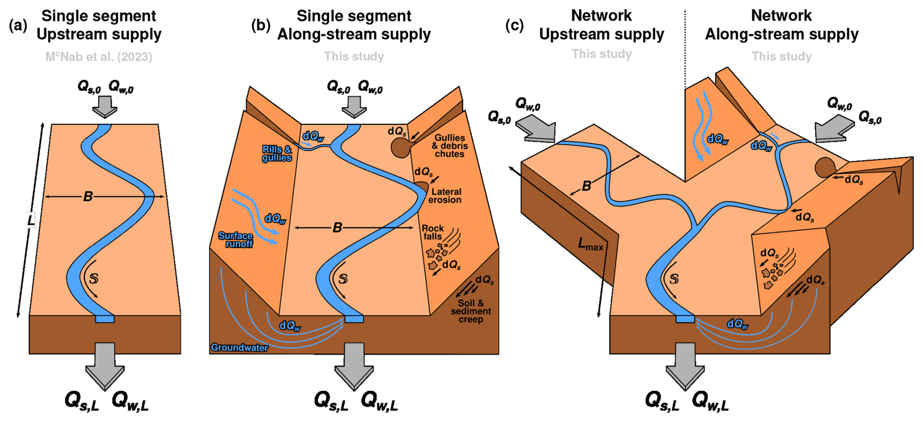
Figure 3 Schematic diagrams showing the alluvial valley cases we investigate. (a) Single-segment, upstream supply case (McNab et al., 2023). Sediment and water are supplied only at the valley inlet, with discharges of Q_s,0 and Q_w,0, respectively. Sediment is transported downstream to the outlet, where it is exported with a discharge of Q_s,L. We assume that changes in water supply affect the entire valley instantaneously, so that the water discharge at the outlet equals that at the inlet, Q_w,0. Also shown are the valley length, L, valley width, B, and channel sinuosity, 𝕊. (b) Single-segment, along-stream supply case. Here, in addition to sediment and water supplied to the inlet, sediment and water are added to the valley continuously along stream. Responsible processes could include: sediment supply from low order gullies and debris chutes, creep and mass wasting on hillslopes, or lateral erosion by the channel; water supply from low order gullies and rills, surface runoff, or groundwater. Since water accumulates along stream, water discharge at the outlet, Q_w,L now diverges from that at the inlet. (c) Network case. Analogous to the single-segment cases, we investigate both an upstream supply case, in which water and sediment and supplied only at valley inlet segments, and an along-stream supply case in which sediment and water are supplied along segments as well as at inlet segments.

Combining Eqs. (1) and (2) gives

$$\begin{array}{}\text{(3)}& {\displaystyle \frac{\partial z}{\partial t}}={\displaystyle \frac{k_{Q_{\mathrm{s}}}I}{{\mathbb{S}}^{\mathrm{7}/\mathrm{6}}B(\mathrm{1}-{\mathit{\lambda }}_{\mathrm{p}})}}{\displaystyle \frac{\partial }{\partial x}}\left(Q_{\mathrm{w}}{\displaystyle \frac{\partial z}{\partial x}}{\left|{\displaystyle \frac{\partial z}{\partial x}}\right|}^{\mathrm{1}/\mathrm{6}}\right)+U,\end{array}$$

a non-linear diffusion equation, in which we have assumed that $k_{Q_{\mathrm{s}}}$, I, and 𝕊 do not vary along stream. Throughout this work, we solve Eq. (3) using the boundary conditions:

$$\begin{array}{}\text{(4)}& {\displaystyle \frac{\partial z}{\partial x}}{|}_{x=\mathrm{0}}=-\mathbb{S}{\left({\displaystyle \frac{Q_{\mathrm{s},\mathrm{0}}}{k_{Q_{\mathrm{s}}}I{Q}_{\mathrm{w},\mathrm{0}}}}\right)}^{\mathrm{6}/\mathrm{7}}\end{array}$$

and

$$\begin{array}{}\text{(5)}& z(x=L,t)=\mathrm{0}.\end{array}$$

Additionally, for single-segment models, we apply the initial condition:

$$\begin{array}{}\text{(6)}& z(x,t=\mathrm{0})=\stackrel{\mathrm{‾}}{z}=-\mathbb{S}{\left({\displaystyle \frac{Q_{\mathrm{s},\mathrm{0}}}{k_{Q_{\mathrm{s}}}I{Q}_{\mathrm{w},\mathrm{0}}}}\right)}^{\mathrm{6}/\mathrm{7}}(L-x),\end{array}$$

where L is the x (i.e., down-valley) position of the valley outlet. Equation (4) states that the slope at the valley inlet is set by the ratio of the sediment and water supplies (denoted Q_s,0 and Q_w,0, respectively). Equation (5) states that the elevation at the valley outlet is fixed to zero. Equation (6) states that the long profile begins in equilibrium with the supplied sediment to water ratio.

2.2 Solutions for a single-segment valley with upstream supply of water and sediment

McNab et al. (2023) explored the behaviour of Eq. (3) for the simple, single-segment case in which all water and sediment is supplied at the valley inlet (Fig. 3a). They showed that, if the system is subjected to small variations in water and sediment supply, such that

$$\begin{array}{}\text{(7)}& Q_{\mathrm{w}}(x,t)=\stackrel{\mathrm{‾}}{Q_{\mathrm{w}}}+\mathit{\delta }{Q}_{\mathrm{w}}\left(t\right)\end{array}$$

and

$$\begin{array}{}\text{(8)}& Q_{\mathrm{s},\mathrm{0}}\left(t\right)=\stackrel{\mathrm{‾}}{Q_{\mathrm{s},\mathrm{0}}}+\mathit{\delta }{Q}_{\mathrm{s},\mathrm{0}}\left(t\right),\end{array}$$

where

$$\begin{array}{}\text{(9)}& \mathit{\delta }{Q}_{\mathrm{w}}\left(t\right)\ll \stackrel{\mathrm{‾}}{Q_{\mathrm{w}}}\end{array}$$

and

$$\begin{array}{}\text{(10)}& \mathit{\delta }{Q}_{\mathrm{s},\mathrm{0}}\left(t\right)\ll \stackrel{\mathrm{‾}}{Q_{\mathrm{s},\mathrm{0}}},\end{array}$$

then variation in elevation can be approximated by

$$\begin{array}{}\text{(11)}& {\displaystyle \frac{\partial \mathit{\delta }z}{\partial t}}\approx \mathit{\kappa }{\displaystyle \frac{{\partial }^{\mathrm{2}}\mathit{\delta }z}{\partial x^{\mathrm{2}}}},\end{array}$$

where

$$\begin{array}{}\text{(12)}& \mathit{\kappa }={\displaystyle \frac{\mathrm{7}}{\mathrm{6}}}{\displaystyle \frac{k_{Q_{\mathrm{s}}}I\stackrel{\mathrm{‾}}{Q_{\mathrm{w}}}}{B(\mathrm{1}-{\mathit{\lambda }}_{\mathrm{p}})}}{\left|{\displaystyle \frac{\partial \stackrel{\mathrm{‾}}{z}}{\partial x}}\right|}^{\mathrm{1}/\mathrm{6}},\end{array}$$

where κ is a sediment-transport diffusivity. In Eqs. (7)–(12), overlines indicate mean values (with respect to time), while “δ”s indicate small variations about those means. Note that, while variations in sediment supply are imposed only at the valley inlet, changes in water supply are assumed to affect the entire valley instantaneously (Eqs. 7–8).

McNab et al. (2023) further showed that if sinusoidal fluctuations in water and sediment supply are imposed, so that

$$\begin{array}{}\text{(13)}& \mathit{\delta }{Q}_{\mathrm{w}}\left(t\right)={\mathcal{A}}_{Q_{\mathrm{w}}}\stackrel{\mathrm{‾}}{Q_{\mathrm{w}}}\sin \left({\displaystyle \frac{\mathrm{2}\mathit{\pi }t}{P}}\right)\end{array}$$

and

$$\begin{array}{}\text{(14)}& \mathit{\delta }{Q}_{\mathrm{s},\mathrm{0}}\left(t\right)={\mathcal{A}}_{Q_{\mathrm{s},\mathrm{0}}}\stackrel{\mathrm{‾}}{Q_{\mathrm{s},\mathrm{0}}}\sin \left({\displaystyle \frac{\mathrm{2}\mathit{\pi }t}{P}}\right),\end{array}$$

then resulting fluctuations in elevation and sediment discharge are approximated by

$$\begin{array}{}\text{(15)}& \mathit{\delta }z(x,t)\approx \stackrel{\mathrm{‾}}{z}({\mathcal{A}}_{Q_{\mathrm{s},\mathrm{0}}}-{\mathcal{A}}_{Q_{\mathrm{w}}})G_z\sin \left({\displaystyle \frac{\mathrm{2}\mathit{\pi }}{P}}\left(t-{\mathit{\phi }}_z\right)\right)\end{array}$$

and

$$\begin{array}{}\text{(16)}& \begin{array}{rl}\mathit{\delta }{Q}_{\mathrm{s}}& (x,t)\approx \\ & \stackrel{\mathrm{‾}}{Q_{\mathrm{s},\mathrm{0}}}({\mathcal{A}}_{Q_{\mathrm{s},\mathrm{0}}}-{\mathcal{A}}_{Q_{\mathrm{w}}})G_{Q_{\mathrm{s}}}\sin \left({\displaystyle \frac{\mathrm{2}\mathit{\pi }}{P}}\left(t-{\mathit{\phi }}_{Q_{\mathrm{s}}}\right)\right).\end{array}\end{array}$$

${\mathcal{A}}_{Q_{\mathrm{s},\mathrm{0}}}$ and ${\mathcal{A}}_{Q_{\mathrm{w}}}$ are dimensionless amplitudes, normalised by their mean values, of sediment supply and water discharge, respectively, while P is the period of the imposed signal. The valley's response to sinusoidal variations in water and sediment supply is itself approximately sinusoidal, modulated by two parameters: “gain”, G_z and $G_{Q_{\mathrm{s}}}$, and phase shift, φ_z and ${\mathit{\phi }}_{Q_{\mathrm{s}}}$ (Howard, 1982, obtained a similar result for a generic linear system). Gain describes the response amplitude relative to the amplitude of the imposed signal. A value of zero indicates that, despite imposed variation in water or sediment supply, there is no variation in elevation or sediment discharge. A value between zero and one indicates that amplitudes of variation in elevation or sediment discharge are lower than those imposed (i.e., the signal is damped, or buffered). A value of one indicates that the response and imposed signal have the same amplitude, while a value greater than one indicates the that imposed signal is amplified. The phase shift, or lag, describes the offset in time between the imposed signal and the valley response.

McNab et al. (2023) provided analytical expressions for G_z, $G_{Q_{\mathrm{s}}}$, φ_z and ${\mathit{\phi }}_{Q_{\mathrm{s}}}$, and showed that they are principally controlled by two key parameters: the relative distance along stream, $x/L$, and the forcing period relative to the valley's equilibration time, $P/T_{\text{eq}}$, where $T_{\text{eq}}=L^{\mathrm{2}}/\mathit{\kappa }$ (e.g., Paola et al., 1992). This result implies that for a given external forcing, the likelihood of terrace formation, related to G_z, and its timing, related to φ_z, depend on the timescale of that forcing, the size of the system, and the position along stream. Similarly, the likelihood of a detectable signal reaching downstream sedimentary basins, related to $G_{Q_{\mathrm{s}}}$ at the valley outlet, and its timing, related to ${\mathit{\phi }}_{Q_{\mathrm{s}}}$ at the outlet, also depend on the forcing timescale and the system size.

3 Approach

Here, we extend McNab et al. (2023)'s application of Wickert and Schildgen (2019)'s model to explore how along-stream sources of water and sediment and the geometries of alluvial valley networks influence their responses to changing water and sediment supply. In turn, we explore how distributions of terraces and their ages within valley networks, as well as patterns of sediment accumulation in downstream basins, are related to external change. Specifically, complementing McNab et al. (2023)'s analysis of the single-segment, upstream supply case, we analyse numerical simulations of two additional geometric representations of a river system (Fig. 3). In the first geometric representation, we model a single-segment valley in which water and sediment are supplied along stream so that they increase continuously according to a power law (hereafter the “single-segment, along-stream supply” case; Fig. 3b). In the second geometric representation, we model branching networks of converging tributaries, including a general case where all sediment and water are supplied at inlet segments and a general case where sediment and water are also supplied along stream (Fig. 3c). For each of these scenarios, we impose periodic variations in sediment and water supply, and compute resulting variations in elevation and sediment discharge along stream and throughout the network. From these results, we derive estimates of gain and phase shift along stream and throughout the network, and compare them to the analytical solutions of McNab et al. (2023) for the single-segment, upstream supply case. This approach allows us to characterise the valley response and isolate the influences of along-stream sediment and water sources and of network geometry.

4 Single-segment valleys with along-stream supply of water and sediment

4.1 Modelling framework

We supply water along stream so that water discharge increases continuously according to a power law:

$$\begin{array}{}\text{(17)}& Q_{\mathrm{w}}=k_{x,Q_{\mathrm{w}}}(x+x_{\mathrm{0}}{)}^{p_{x,Q_{\mathrm{w}}}},\end{array}$$

where $k_{x,Q_{\mathrm{w}}}$ is the power-law coefficient linking distance downstream to bankfull water discharge, $p_{x,Q_{\mathrm{w}}}$ is the power-law exponent, and x₀ is a distance from the drainage divide at the valley inlet. This approach is similar to that of several previous studies (e.g., Goldberg et al., 2021; Braun, 2022). Equation (17) is related to Hack's Law, which connects downstream distance to upstream drainage area (though commonly expressed in the opposite sense, with downstream distance as a function of drainage area; Hack, 1957). However, the relationship between drainage area and bankfull water discharge is not linear, being influenced, for example, by catchment hydrology and the catchment's size relative to that of the footprint of major rainfall events (Sólyom and Tucker, 2004). These effects result in bankfull water discharge increasing more slowly downstream than drainage area (Aron and Miller, 1978; O'Connor and Costa, 2004). We adapt the earlier definitions of equilibration time, T_eq, (e.g., Paola et al., 1992) to account for along-stream variation in water discharge as follows:

$$\begin{array}{}\text{(18)}& T_{\text{eq}}={\displaystyle \frac{L^{\mathrm{2}}}{\langle \mathit{\kappa }\rangle }},\end{array}$$

where the angled brackets indicate a spatial average.

In an extension to previous studies, we also supply sediment along stream. We set the source term, U, in Eq. (3), to the sediment supply per unit distance along stream. We choose this along-stream sediment supply so that sediment discharge at steady state also increases downstream according to a power law with the same form as Eq. (17). As such,

$$\begin{array}{}\text{(19)}& \begin{array}{rl}U& ={\displaystyle \frac{\mathrm{1}}{B(\mathrm{1}-{\mathit{\lambda }}_{\mathrm{p}})}}{\displaystyle \frac{\partial Q_{\mathrm{s}}}{\partial x}}={\displaystyle \frac{k_{x,Q_{\mathrm{s}}}{p}_{x,Q_{\mathrm{s}}}(x+x_{\mathrm{0}}{)}^{p_{x,Q_{\mathrm{s}}}-\mathrm{1}}}{B(\mathrm{1}-{\mathit{\lambda }}_{\mathrm{p}})}}\\ & ={\displaystyle \frac{\mathrm{1}}{B(\mathrm{1}-{\mathit{\lambda }}_{\mathrm{p}})}}{\displaystyle \frac{Q_{\mathrm{s},\mathrm{0}}}{Q_{\mathrm{w},\mathrm{0}}}}{\displaystyle \frac{\partial Q_{\mathrm{w}}}{\partial x}}.\end{array}\end{array}$$

4.2 Numerical simulations

We simulate five single-segment valleys in which sediment and water discharge increase at different rates, with $\mathrm{0.8}\le (p_{x,Q_{\mathrm{w}}}=p_{x,Q_{\mathrm{s}}})\le \mathrm{2.4}$ (Fig. 4a). This range corresponds approximately to an inverse Hack's law exponent in the range 1.6–2.4 (typical values from global compilations, e.g. Shen et al., 2017; He et al., 2024), combined with an exponent linking drainage area to bankfull water discharge in the range 0.5–1 (Aron and Miller, 1978; O'Connor and Costa, 2004; Sólyom and Tucker, 2004). For each valley, we choose $k_{x,Q_{\mathrm{w}}}$ and $k_{x,Q_{\mathrm{s}}}$ so that the ratio of sediment to water discharge remains constant along stream at steady state and the average water and sediment discharge is equal across all five simulated valleys (specifically, we set the spatial and temporal mean water discharge, $\langle \stackrel{\mathrm{‾}}{Q_{\mathrm{w}}}\rangle$, to 26 m³ s⁻¹, and supply sediment from upstream and along stream such that the spatial and temporal mean sediment discharge, $\langle \stackrel{\mathrm{‾}}{Q_{\mathrm{s}}}\rangle$, is $\mathrm{2.6}\times {\mathrm{10}}^{-\mathrm{3}}$ m³ s⁻¹). As such, each valley has the same steady-state slope, which is constant along stream (Fig. 4b). We set valley width, B, to a uniform value of 256 m, so that each valley has the same equilibration time of 100 kyr (as defined in Eq. 18).

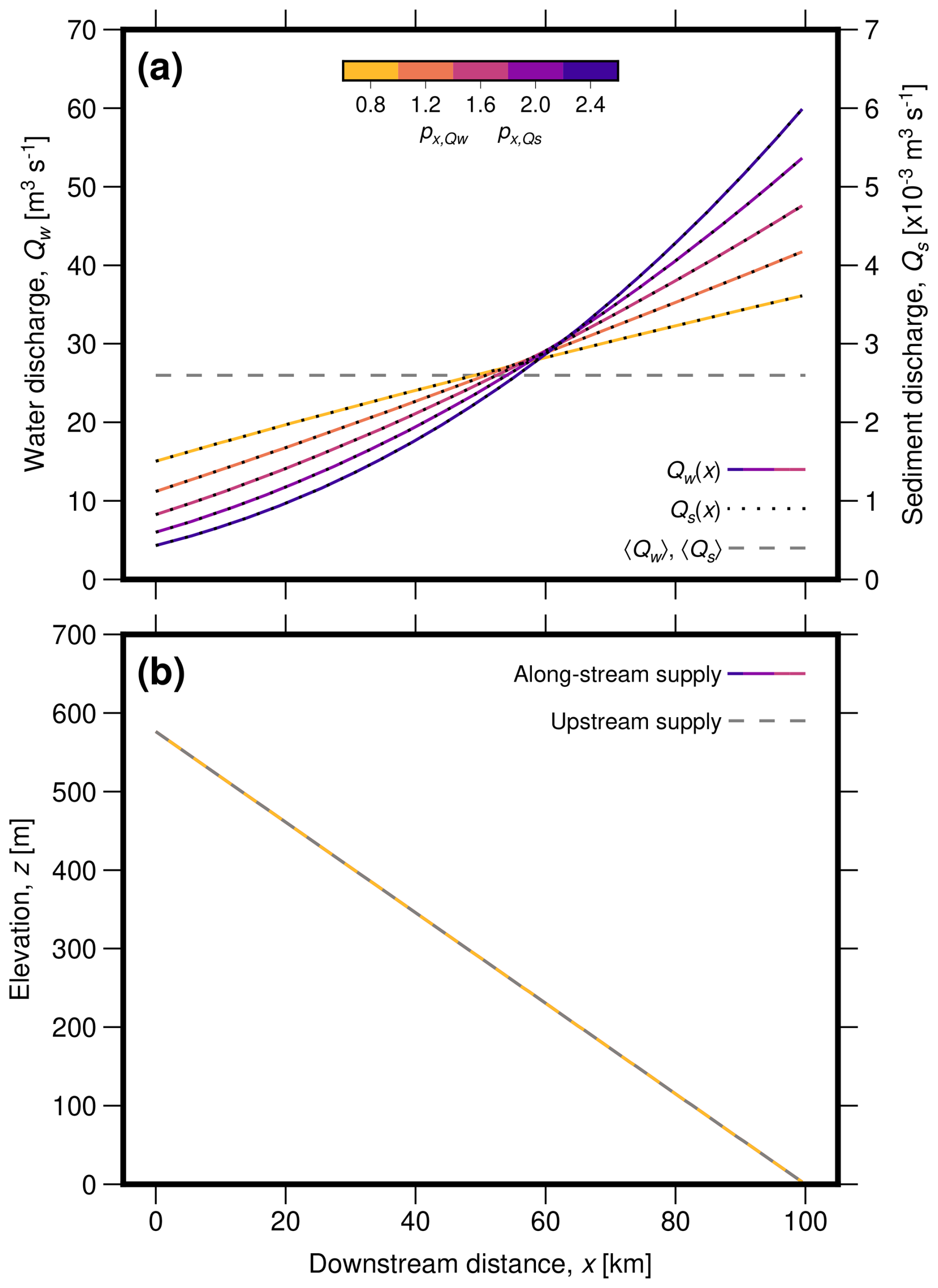
Figure 4 Initial setup for case with along-stream supply of water and sediment, and comparison with the upstream supply case. (a) Water discharge, Q_w, (solid lines) and sediment discharge, Q_s (dotted lines), as functions of distance downstream, where colour indicates power-law exponents $p_{x,Q_{\mathrm{w}}}=p_{x,Q_{\mathrm{s}}}$. Dashed grey line shows spatial average, corresponding to the upstream supply case. (b) Elevation as a function of distance downstream for the case with along-stream supply of water and sediment (solid lines) and the case with only upstream supply of water and sediment (dashed line). Since the ratio of sediment to water discharge is held constant throughout the domain and between each valley, the profiles are linear with the same slope as one another.

For each valley, we performed a series of numerical simulations in which we varied sediment or water supply sinusoidally (both at the inlet and along stream), with a range of periods between $P/T_{\text{eq}}={\mathrm{10}}^{-\mathrm{2}}$–10². We define gain numerically as

$$\begin{array}{}\text{(20)}& G_z\left(x\right)={\displaystyle \frac{max\left(z\right(x,t\left)\right)-min\left(z\right(x,t\left)\right)}{\mathrm{2}\stackrel{\mathrm{‾}}{z\left(x\right)}({\mathcal{A}}_{Q_{\mathrm{s}}}-{\mathcal{A}}_{Q_{\mathrm{w}}})}}\end{array}$$

and

$$\begin{array}{}\text{(21)}& G_{Q_{\mathrm{s}}}\left(x\right)={\displaystyle \frac{max\left(Q_s\right(x,t\left)\right)-min\left(Q_s\right(x,t\left)\right)}{\mathrm{2}\stackrel{\mathrm{‾}}{Q_s\left(x\right)}({\mathcal{A}}_{Q_{\mathrm{s}}}-{\mathcal{A}}_{Q_{\mathrm{w}}})}},\end{array}$$

which we compute directly from the simulated time series of elevation and sediment discharge. To avoid the influence of transient effects at the onset of periodic forcing, we measure gain only after two complete cycles (i.e., with t>2P). We estimate the phase shift by extracting peaks and troughs in the simulated time series of elevation and sediment discharge and measuring the difference in time between them and peaks and troughs in the imposed signal. We then explore how gain and lag vary along stream, as functions of forcing period and discharge exponent, and compare with equivalent results for the single-segment, upstream supply case (derived from numerical simulations and analytical solutions previously presented by McNab et al., 2023).

4.3 Results and comparison with single-segment, upstream-supply case

We first show simulated aggradation, incision and sediment discharge of an example valley with $p_{x,Q_{\mathrm{w}}}=p_{x,Q_{\mathrm{s}}}=\mathrm{1.6}$ at three forcing periods (Fig. 5). For comparison, we also include results from an equivalent simulation with sediment and water supplied only upstream (i.e., with $p_{x,Q_{\mathrm{w}}}=p_{x,Q_{\mathrm{s}}}=\mathrm{0}$; McNab et al., 2023). To elucidate further how the valley response varies spatially, with forcing timescale, and with the power-law exponent, we then show gain and lag for each valley as functions of downstream distance (Fig. 6) and forcing period (Fig. 7), again with comparison to the upstream supply case (McNab et al., 2023). We found that, in all cases, patterns of long-profile evolution are similar regardless of whether sediment supply or water supply is varied. We therefore only show variation in elevation driven by variation in sediment supply here (equivalent results for variation in water supply are shown in Figs. S1–S3 in the Supplement). To further simplify the presentation of results, while we consider how the long profile varies along stream, we focus on variation in sediment discharge only at the valley outlet, which is most relevant for downstream sedimentary basins.

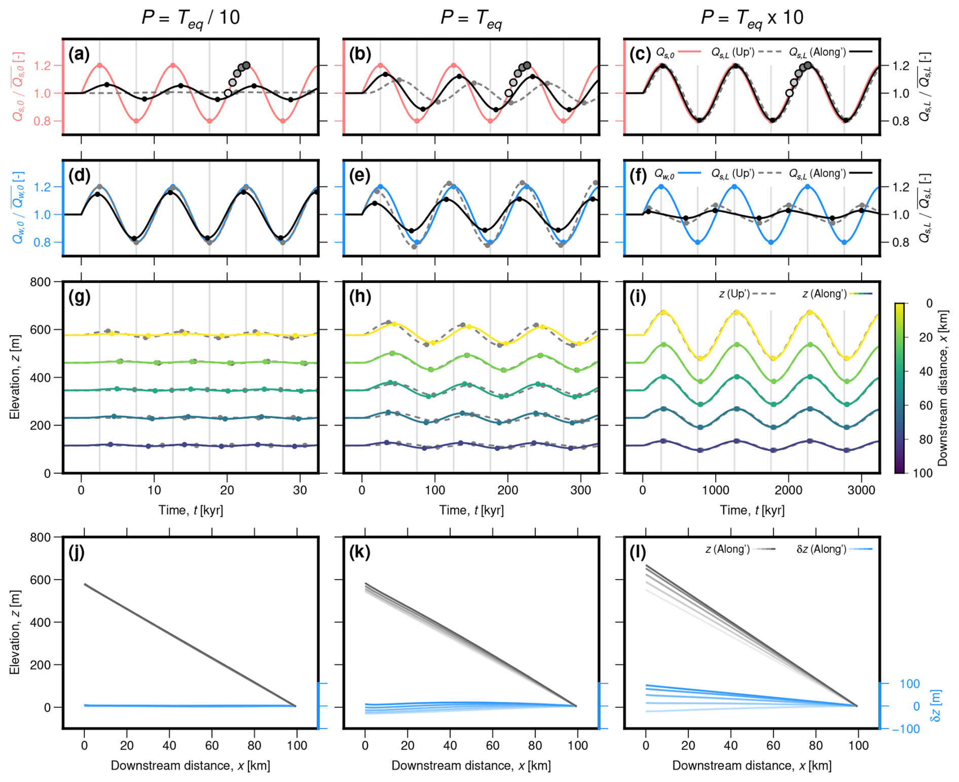
Figure 5 Valley response to sinusoidal variation in sediment and water supply at three forcing periods, for the cases where all sediment and water are supplied at the valley inlet (dashed lines, previously shown by McNab et al., 2023) and where sediment and water are supplied along stream with a power-law exponent $p_{x,Q_{\mathrm{w}}}=p_{x,Q_{\mathrm{s}}}=\mathrm{1.6}$. (a–c) Red solid line shows normalised variation in sediment supply as a function of time; dashed grey line shows normalised sediment discharge at the valley outlet for the upstream-supply case; solid black line shows normalised sediment discharge at the valley outlet for the along-stream supply case; greyscale circles show times used in panels (j–l). (d–f) Same as (a–c) except blue solid line shows normalised variation in water supply. (g–i) Elevation, z, as a function of time for selected positions along stream, in response to changing sediment supply. Dashed grey lines represent upstream-supply case; solid, coloured lines represent along-stream supply case. (j–l) Valley long profiles at different times for the along-stream supply case in response to changing sediment supply (for the upstream supply case, compare with Figs. 2 and 3 in McNab et al., 2023). Grey scale lines show long profiles, where shade corresponds to times represented by circles on panels (a–c); bluescale lines show perturbations from the steady state profile, δz. Equivalents to panels (g–l) for variation in water supply are shown in Fig. S1.

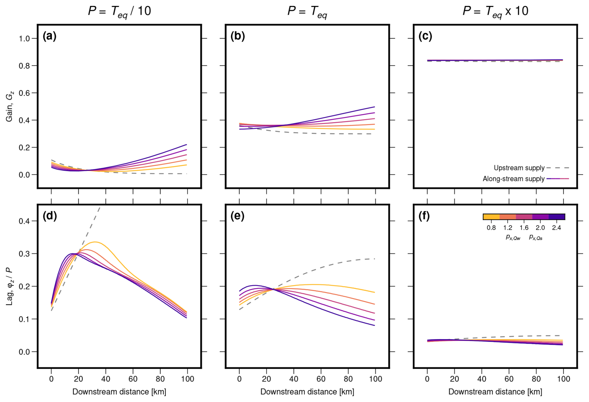
Figure 6 Elevation gain, G_z, and lag, φ_z, of valley response to changing sediment supply, as functions of distance downstream for three forcing periods, $P=T_{\text{eq}}/\mathrm{10}$ (a, d); P=T_eq (b, e); $P=T_{\text{eq}}\times \mathrm{10}$ (c, f). Dashed grey lines show G_z and φ_z for the case where all sediment and water is supplied at the valley inlet (computed using the analytical expression given by McNab et al., 2023). Solid lines show G_z and φ_z for the case where sediment and water are supplied continuously along stream, where colour represents power-law exponent $p_{x,Q_{\mathrm{w}}}=p_{x,Q_{\mathrm{s}}}$. Note that the saturation of G_z at $\mathrm{6}/\mathrm{7}$ is related to the power of $\mathrm{7}/\mathrm{6}$ in the sediment-transport equation (Eq. 2). The behaviour in response to changing water supply is very similar (Fig. S2).

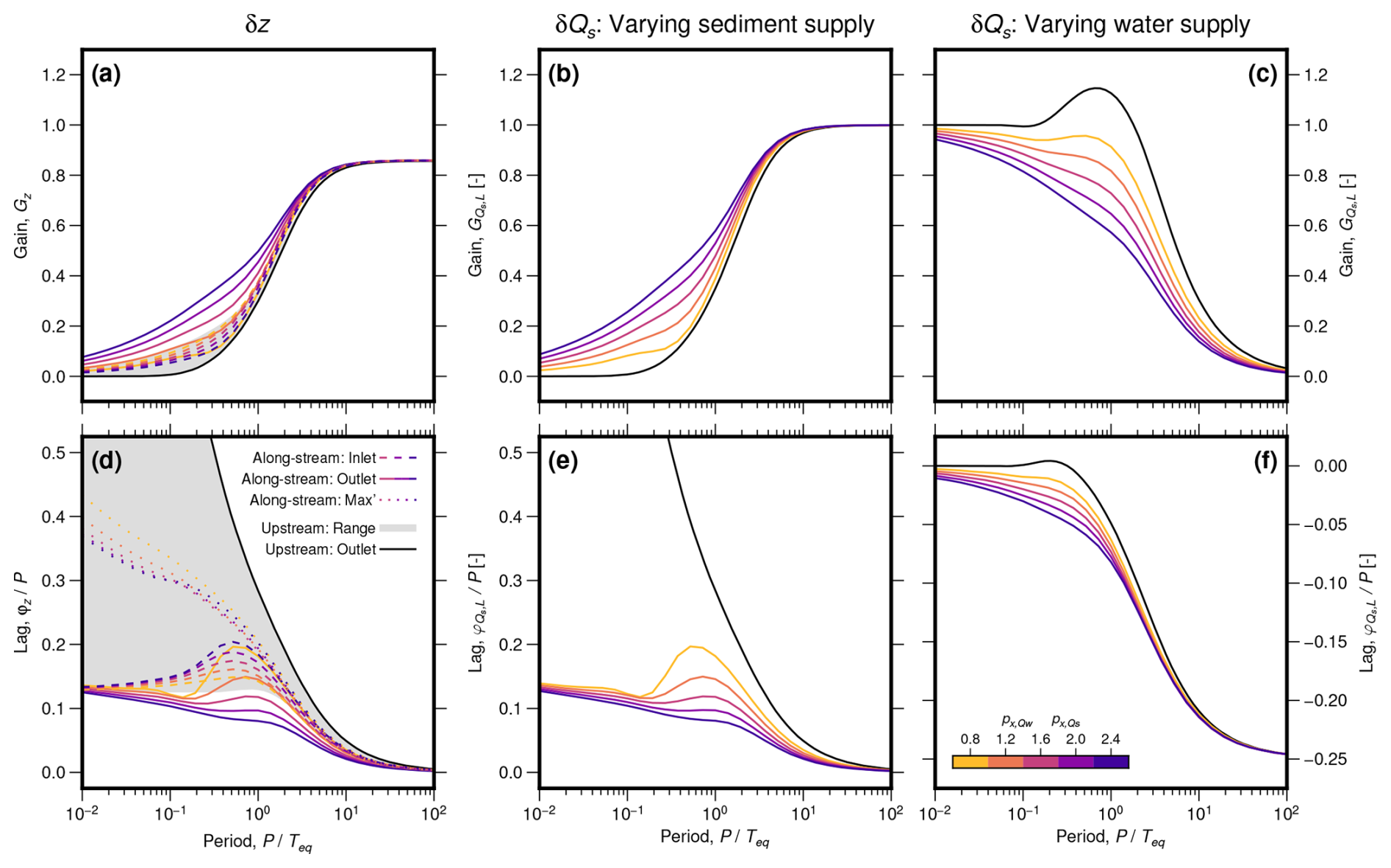
Figure 7 Gain and lag as functions of forcing period. (a) Elevation gain, G_z, as a function of forcing period, P. Black line and grey band show G_z at the valley outlet and its range throughout the valley, respectively, for the upstream supply case (computed using the analytical expression given by McNab et al., 2023). Solid and dashed coloured lines show G_z at the valley outlet and inlet, respectively, for the along-stream supply case, where colour represents power-law exponent $p_{x,Q_{\mathrm{w}}}=p_{x,Q_{\mathrm{s}}}$. (b, c) As (a) for variation in sediment discharge at the outlet, $G_{Q_{\mathrm{s},L}}$, in response to varying sediment and water supply, respectively. (d) As (a) for elevation lag, φ_z. Additionally, dotted lines show maximum φ_z measured at any position along the valley for the along-stream supply case. Equivalents to panels (a) and (d) for variation in water supply are shown in Fig. S3. (e, f) As (d) for variation in sediment discharge at the outlet, ${\mathit{\phi }}_{Q_{\mathrm{s},L}}$, in response to varying sediment and water supply, respectively.

Broad patterns of aggradation and incision are similar for both the upstream and along-stream supply cases (Figs. 5g–l, 6 and 7a and d; see also Howard, 1982; Goldberg et al., 2021; Braun, 2022). In both cases, when the forcing period is short relative to the valley's equilibration time (P≪T_eq), amplitudes of aggradation and incision are low (G_z≈0) and lag significantly behind the forcing (φ_z>0). At intermediate forcing periods (P≈T_eq), amplitudes are increased and lag times reduced. When forcing periods significantly exceed the equilibration time (P≫T_eq), aggradation and incision occurs with similar amplitudes to, and close to in phase with, the imposed variation in sediment or water supply ($G_z\approx \mathrm{6}/\mathrm{7}\approx \mathrm{0.86}$, φ_z≈0; the value of $\mathrm{6}/\mathrm{7}$ is related to the $\mathrm{7}/\mathrm{6}$ power on valley slope in the sediment-discharge equation, Eq. 2).

Nevertheless, some important differences in patterns of aggradation and incision do arise between the upstream and along-stream supply cases, most evident in the distributions of gain and lag as functions of downstream distance and forcing period (Figs. 6 and 7). First, in the along-stream supply case, G_z is larger and φ_z is generally lower than in the upstream supply case, for a given forcing period. Second, in the upstream supply case, G_z and φ_z decrease and increase continuously downstream, respectively (Fig. 6). In contrast, in the along-stream supply case, while G_z initially decreases and φ_z increases away from the inlet, both reach turning points so that G_z increases and φ_z decreases towards the outlet. Third, while in the upstream supply case φ_z decreases continuously as the forcing period increases, in the along-stream supply case, it briefly increases to a maximum for periods close to the valley's equilibration time (P≈T_eq; Fig. 7d). These differences generally become more pronounced as the water- and sediment-discharge power-law exponents increase (Figs. 6 and 7).

When sediment supply is varied, variation in sediment output follows similar patterns to aggradation and incision (Figs. 5a–c and 7b and e); however, when water supply is varied, different behaviour emerges (Figs. 5d–f and 7c and f; cf. Simpson and Castelltort, 2012; Goldberg et al., 2021; Braun, 2022). When the period of variation in water supply is short relative to the valley's equilibration time (P≪T_eq), variation in sediment output has the same amplitude and is in phase with the forcing ($G_{Q_{\mathrm{s}}}=\mathrm{1}$, ${\mathit{\phi }}_{Q_{\mathrm{s}}}=\mathrm{0}$). In the upstream supply case, when the forcing period is increased, the amplitude of variation in sediment output briefly exceeds that of the imposed variation in water supply ($G_{Q_{\mathrm{s}}}>\mathrm{1}$ while P≈T_eq), before decreasing to zero for long forcing periods. In the along-stream supply case, variation in sediment output is not amplified at periods close to the valley's equilibration time, instead decreasing continuously as the forcing period increases. In both cases, negative lag times are introduced, so that peaks in sediment output precede corresponding peaks in water supply.

4.4 Interpretation

Two concepts help explain physically the variations in valley response that arise due to changing sediment and water supply (Figs. 5–7). First, the extent to which the valley can adjust to external perturbations depends on the relationship between the perturbation timescale and the timescale over which the valley can aggrade and incise (e.g., Howard, 1982; Paola et al., 1992; Goldberg et al., 2021; Braun, 2022). At the valley scale, the approximate timescale over which the valley can adjust is given by the equilibration time, T_eq. At the local scale, however, the adjustment efficiency is also influenced by the local diffusivity (Eq. 12). In the upstream case, diffusivity is uniform along the valley, while in the along-stream supply case, it increases downstream with water discharge, so that the capacity for the valley to adjust also increases downstream. Second, variation in sediment and water supply can be thought of as a signal introduced to the valley that can propagate along stream. In the upstream supply case, this signal takes the form of variations in slope at the inlet, that must then propagate downstream. In the along-stream supply case, as well as signal originating from the valley inlet, signal is introduced continuously along the valley, and propagates both up- and down-stream.

We first apply these concepts to patterns of aggradation and incision (Figs. 5g–l, 6 and 7a and d). At the valley scale, when sediment or water supply vary with periods much smaller than T_eq, aggradation and incision cannot keep pace with the forcing and amplitudes are low. As the forcing period increases to values similar to or greater than T_eq, aggradation and incision can increasingly keep pace and amplitudes increase. In the upstream supply case, signal is introduced only at the inlet, so that lag increases continuously downstream as the signal propagates. For short forcing periods relative to T_eq, incomplete adjustment causes the signal to diffuse as it propagates, so that gain decreases downstream. In contrast, in the along-stream supply case, signal is introduced continuously along stream, and diffusivity increases downstream as a result of increasing water discharge. As such, downstream parts of the valley do not need to “wait” for signal to propagate from the inlet, and have a greater capacity to adjust to the forcing. Away from the inlet, local signal sources therefore increasingly dominate, so that gain increases and lag decreases towards the outlet (i.e., the signal appears to propagate upstream).

Peaks in lag at forcing periods close to T_eq for the along-stream case reflect the interaction between local and upstream signal sources (Fig. 7d). At shorter forcing periods, signal introduced at the inlet quickly diffuses away, so that aggradation and incision further downstream is controlled only by local signal sources. At periods around T_eq, signal introduced at the inlet maintains some amplitude downstream, but takes time to propagate; the increasing influence of this upstream signal causes lag times to increase briefly with increasing period. As the forcing period increases further, the signal propagates more efficiently downstream, so that lag times again steadily decrease.

When sediment supply is varied, variation in sediment discharge is driven only by variation in valley slope (Eq. 2). Thus, in both the upstream and along-stream supply cases, variation in sediment output closely follows that of aggradation and incision at the valley outlet: $G_{Q_{\mathrm{s}}}$ and ${\mathit{\phi }}_{Q_{\mathrm{s}}}$ behave similarly to G_z and φ_z (Figs. 5a–c and 7b and e).

In contrast, when water supply is varied, it influences the valley's capacity to transport sediment directly as well as triggering variations in slope (Eq. 2). Interactions can then arise between the imposed variation in water supply and the resulting variations in slope that can be damped and lag behind the forcing (Figs. 5a–c and 7b and e). At forcing periods much shorter than T_eq, slopes do not adjust along much of the valley, so that variation in water supply is translated directly into to variation in sediment output. Meanwhile, at forcing periods much longer than T_eq, slopes can adjust to maintain an equilibrium with sediment and water supply, so that sediment output varies little (see also Goldberg et al., 2021; Braun, 2022). At intermediate forcing periods, slopes partially adjust, but lag behind the imposed variation in water supply. In the upstream supply case, variation in water supply and slope combine to amplify the imposed signal, while in the along-stream supply case, amplitudes simply decrease from short to long forcing periods.

In both the upstream and along-stream supply cases, the delayed adjustment of valley slope leads to a negative lag in sediment output, such that peaks in sediment output arise prior to imposed peaks in water supply (Figs. 5d–f and 7f). Consider the onset of sinusoidal variation in water supply. Initially, water supply increases without any adjustment of valley slope, so that sediment output also increases. Valley slope then begins to decrease, so that sediment output increases more slowly and then begins to decrease. This transition occurs prior to water supply reaching its maximum, resulting in the negative lag or appearance that variation in sediment output leads that of water supply.

5 Alluvial valley networks

5.1 Modelling framework

We model alluvial valley networks as a series of interconnected network segments, each of which follow Eq. (3). We supply sediment and water to inlet segments (i.e., segments without any segments upstream), and impose base level at the outlet segment (i.e., a segment without any segments downstream). In some cases, we also supply water and sediment along stream, analogously to the single segment, along-stream supply case presented above (Fig. 3c). Within the network, a segment's sediment supply is set by the sum of sediment discharges from its upstream segments, while elevation is required to be continuous across segment junctions (see also Howard, 1982). To solve Eq. (3), we use the semi-implicit finite-difference scheme presented by Wickert and Schildgen (2019) adapted for a network (Wickert et al., 2025).

To define the network topology (i.e., the position of each segment in the network relative to its adjacent segments), we use an approach introduced by Shreve (1966), following the algorithm outlined by Shreve (1974). This algorithm randomly generates binary trees with a given number of valley inlet (or “exterior”) segments; an example is shown in Fig. 8a–d. The algorithm treats all possible binary trees as equally likely. It has been argued that populations of binary trees generated with this approach are not realistic representations of real river-network populations, because, unlike river networks, the trees produced are not necessarily space filling (e.g., Dodds and Rothman, 2000). Abrahams (1984) discusses observations from real networks that deviate from the predictions of Shreve's model, often associated with space-filling constraints, but also occurring in regions with high relief. We note that several other frameworks for randomly generating synthetic networks have been developed, including, for example: undirected or directed random walks on lattices (Leopold and Langbein, 1962; Scheidegger, 1967); models of headward growth and branching (Howard, 1971; Dunkerley, 1977); “Random Self-similar Networks”, that can be constructed with specified statistical properties (Veitzer and Gupta, 2000); and “Optimal Channel Networks”, that seek to minimise energy expenditure involved in the transport of water across the landscape (Howard, 1990; Rodriíguez-Iturbe et al., 1992). Several of these approaches avoid the space-filling problem by constructing networks explicitly on two-dimensional grids, but no consensus has emerged as to which most successfully recreates realistic network populations. Furthermore, our model of long-profile evolution and sediment transport does not require any spatial information beyond distances along stream and the topological relationships between segments. We therefore persist with Shreve's approach, since it is relatively simple and samples all possible binary trees, with the caveat that the statistics of network populations we obtain may deviate from those of natural networks.

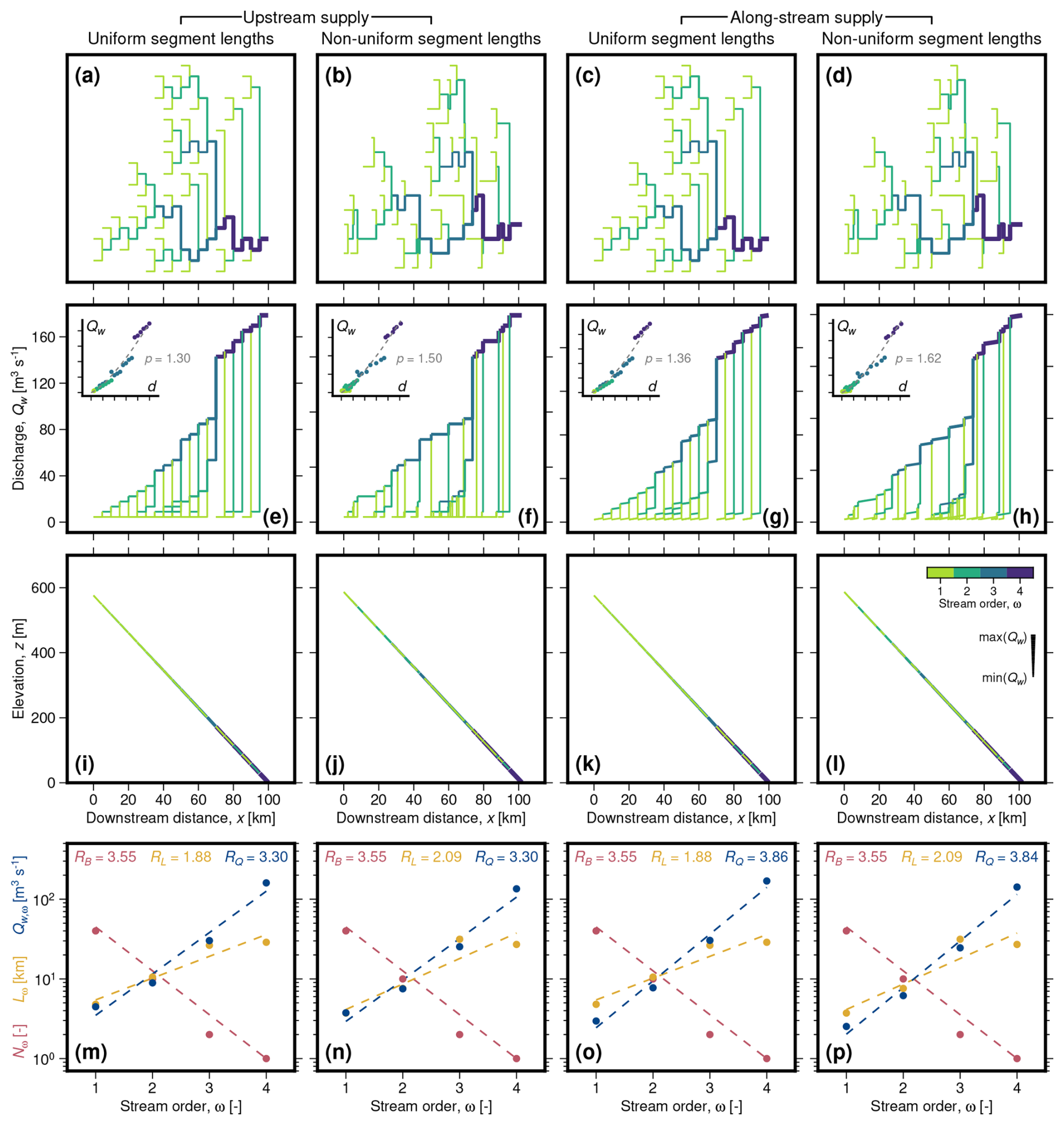
Figure 8 Randomly generated networks for four scenarios: (a, e, i, m) uniform segment lengths with upstream supply of sediment and water; (b, f, j, n) non-uniform segment lengths with upstream supply of sediment and water; (c, g, k, o) uniform segment lengths with along-stream supply of sediment and water; and (d, h, l, p) non-uniform segment lengths with along-stream supply of sediment and water. (a–d) Schematic network planforms, where colour indicates stream order (Strahler, 1952). Horizontal lines represent network segments while vertical lines represent connections between segments and have no physical meaning; the planforms are intended only to illustrate relationships between segments. Line thickness scales with water discharge (see key in panel l). (e–h) Discharge as a function of distance downstream. As in panels (a–d), horizontal lines represent network segments while vertical lines connect segments, and line thickness scales with water discharge. Insets show discharge as a function of distance from furthest valley inlet, d, where circles represent each segment and dashed lines show best fit power-law relationship. Note that discharge axes for the main panel and inset change slightly between each case; ticks are consistently spaced at 40 m³ s⁻¹. (i–l) Longitudinal profiles. Note that, since steady-state slope is consistent across the network, segments with the same downstream distance are superimposed. (m–p) Number of segments (N_ω, red), mean stream lengths (L_ω, yellow) and mean stream discharges (Q_w,ω, blue), as functions of stream order, ω. Circles show measured values; dashed lines show best fit relationships, and their gradients correspond to R_B, R_L, and $R_{Q_{\mathrm{w}}}$, respectively (Eqs. 22–25).

Once the network topology has been defined, lengths and properties such as water discharge and valley width need to be assigned to each segment. In natural networks, segment lengths and widths vary, and water discharge is derived from upstream catchment areas as well as locally from groundwater and surface runoff. Such complexities may influence how alluvial river networks respond to external variation in sediment and water supply, but they may also obfuscate more general aspects of network behaviour. We therefore start with more simplified synthetic representations of alluvial river networks, before progressively building complexity towards more naturalistic representations.

Specifically, we consider four network scenarios. In the simplest scenario, we set segment lengths to a uniform value of 5 km and supply water and sediment only at the valley inlets (Figs. 3c and 8a and e). In the second scenario, we draw random segment lengths from a gamma distribution with a shape parameter of two and a mean of 5 km, following Shreve (1969) and Shreve (1974), but still supply water and sediment only at the valley inlets (Fig. 8b and f). Note that, unlike Shreve (1969) and Shreve (1974), we do not use different length distributions for inlet and interior segments, for simplicity and due to a lack of evidence for systematic differences between them (Abrahams, 1984). Shreve (1974) also showed that a segment's local contributing area scales approximately linearly with its length, with a factor of around 300 m² m⁻¹. In the third scenario, we therefore return to uniform segment lengths, but add water and sediment along each segment as well as at the valley inlets (Figs. 3c and 8c and g). In the fourth scenario, we use non-uniform segment lengths and also add water and sediment along each segment (Fig. 8d and h). In all scenarios, we set values of upstream and along-stream water supply so that the mean across each network, $\langle \stackrel{\mathrm{‾}}{Q_{\mathrm{w}}}\rangle$, is 26 m³ s⁻¹. We also fix the ratio of sediment to water supply to a constant value of 10⁻⁴, and neglect any downstream fining, so that the network long profiles are linear at steady state (Fig. 8i–l; cf. Pizzuto, 1992). We do not expect this choice to influence significantly our results, since the diffusivity is only weakly dependent on valley slope (Eq. 12). In all scenarios, we fix the valley width to a uniform value of 254 m; we return to implications of this choice in the Discussion (Sect. 6.3).

5.2 Characterising network geometries

To explore how a network's geometry influences its response to external forcing, we first need to be able to describe its geometry in a quantitative way. This topic has been the focus of considerable effort for the last few decades, so that many network metrics have been proposed and applied. In the absence of a priori ideas regarding controls on network responses to changing sediment and water supply, we test a range of existing metrics that quantify different aspects of network structure.

Horton (1945) developed an influential set of statistics describing network geometries that are now known as “Horton's laws”. These laws rely on the concept of “stream order”, which was later modified by Strahler (1952). Exterior or inlet segments are defined as first order streams. Where two first order streams combine, a second order stream is formed. Where a second order stream meets a first order stream, the second order stream is lengthened; only when two second order streams meet is a third order stream initiated, and so on. Thus streams of order two or greater can consist of multiple network segments. Horton (1945) showed that, within a given network, the number of streams with order ω, N_ω, decreases with stream order such that

$$\begin{array}{}\text{(22)}& {\displaystyle \frac{N_{\mathit{\omega }}}{N_{\mathit{\omega }+\mathrm{1}}}}\approx R_B\text{, or }{N}_{\mathit{\omega }}\approx {R_B}^{\mathrm{\Omega }-\mathit{\omega }},\end{array}$$

where Ω is the maximum stream order within the network. R_B is termed the “bifurcation ratio”, and can be visualised as the gradient of a linear function relating ω to N_ω in linear-logarithmic space (Fig. 8m–p). Horton (1945) also showed that stream lengths increase with stream order, such that

$$\begin{array}{}\text{(23)}& {\displaystyle \frac{L_{\mathit{\omega }}}{L_{\mathit{\omega }-\mathrm{1}}}}\approx R_L\text{, or }{L}_{\mathit{\omega }}\approx {R_L}^{\mathit{\omega }-\mathrm{1}}\text{.}\end{array}$$

Schumm (1956) showed that a similar rule applies to stream drainage areas:

$$\begin{array}{}\text{(24)}& {\displaystyle \frac{A_{\mathit{\omega }}}{A_{\mathit{\omega }+\mathrm{1}}}}\approx R_A\text{, or }{A}_{\mathit{\omega }}\approx {R_A}^{\mathit{\omega }-\mathrm{1}}.\end{array}$$

L_ω and A_ω are mean lengths and drainage areas, respectively, of streams with order ω; and R_L and R_A are termed the length and area ratios, respectively. Since the synthetic networks used here have no inherent upstream drainage area, we define a related statistic using water discharge:

$$\begin{array}{}\text{(25)}& {\displaystyle \frac{Q_{\mathrm{w},\mathit{\omega }}}{Q_{\mathrm{w},\mathit{\omega }+\mathrm{1}}}}\approx R_{Q_{\mathrm{w}}}\text{, or }{Q}_{\mathrm{w},\mathit{\omega }}\approx {R_{Q_{\mathrm{w}}}}^{\mathit{\omega }-\mathrm{1}},\end{array}$$

where Q_w,ω is mean water discharge of streams with order ω and $R_{Q_{\mathrm{w}}}$ is the discharge ratio. Typical values of Horton's ratio in natural networks are: $\mathrm{3}<R_B<\mathrm{5}$, $\mathrm{1.5}<R_L<\mathrm{3}$ and $\mathrm{3}<R_A<\mathrm{6}$, and Shreve (1966, 1969) showed that populations of random networks generated using his approach (which we adopt here) return similar values. However, Kirchner (1993) showed that these ranges are in fact characteristic of all possible binary trees, while Jarvis and Werritty (1975) showed that Horton's laws retain relatively little information about network topology. Both Jarvis and Werritty (1975) and Kirchner (1993) therefore suggest that Horton's Laws are not particularly useful measures of network structure. Costa-Cobral and Burges (1997) do show, nevertheless, that they can in some cases be used to discriminate between network populations with different characteristics. We include them here for completeness and consistency with the existing literature.

Another limitation of Horton's laws is that they do not distinguish between streams of a given order that flow into streams of different higher orders (e.g., a first-order stream that flows into a second-order stream is treated the same as one that flows into a third order stream). As such, they only hold exactly for networks in which streams of each order exclusively flow into streams exactly one order higher (Tarboton, 1996). Tokunaga (1978) devised an alternative scheme which does account for all possible relationships between streams of different orders. Tokunaga defines the parameter ϵ_i as the average number of streams of order ω flowing into streams of order ω+i. They then define the parameter K as average decrease in ϵ_i as i is incrementally increased, i.e., the average of ${\mathit{ϵ}}_{\mathrm{1}}/{\mathit{ϵ}}_{\mathrm{2}}$, ${\mathit{ϵ}}_{\mathrm{2}}/{\mathit{ϵ}}_{\mathrm{3}}$, …, ${\mathit{ϵ}}_{\mathrm{\Omega }-\mathrm{1}}/{\mathit{ϵ}}_{\mathrm{\Omega }}$. K is therefore a more sophisticated version of Horton's R_B.

Another prominent series of network metrics are built around the concept of “topological length” (e.g., Werner and Smart, 1973; Jarvis and Werritty, 1975). This framework is particularly attractive for the present problem since timescales of diffusive processes are known to scale with a system's length (e.g., Paola et al., 1992). A segment's topological length, which we denote l, is defined as the number of segments from it to the outlet (including it and the outlet segment). Commonly used metrics making use of the topological length are: the maximum topological length of all segments in the network, l_max (also known as the network “diameter”); the average topological length of all segments in the network, 〈l〉; and the average topological length of all inlet segments, 〈l_I〉 (also known as the “mean source height”). Since some of the networks we analyse have variable segment lengths, we also define an equivalent set of metrics that use absolute rather than topological lengths, i.e.: the maximum length to the outlet, L_max; the mean length of all segments in the network to the outlet, 〈L〉; and the mean length from all inlet points to the outlet, 〈L_I〉 (cf. the catchment “centre of gravity”; Langbein, 1947; Gray, 1961).

Similar to the topological length is the concept of “topological width”, defined as the number of segments positioned at a given topological length from the outlet, w (e.g., Kirkby, 1976; Ranjbar et al., 2018). Typically, the maximum topological width in a network, w_max, is taken as a measure of a its structure; we also include the mean topological width, 〈w〉.

Lastly, we make use of the widely documented power-law relationship between upstream drainage area and distance downstream from the drainage divide known as Hack's law (Hack, 1957; Gray, 1961; Mueller, 1972). The exponent of this power law provides a measure of the rate at which drainage area accumulates downstream. As in the case of R_A above, since the networks we analyse have no inherent upstream drainage area, we fit a power-law function relating a point's distance from the furthest inlet to its water discharge (insets in Fig. 8e–h). The exponent of this power law, p, is then equivalent to a combination of an inverse Hack's exponent and an exponent linking drainage area to bankfull water discharge.

5.3 Numerical simulations

For each of the four network scenarios described in Sect. 5.1, we performed two sets of simulations. First, to assess the range of behaviour of networks with a fixed number of segments, we generated 200 networks each with 40 valley inlet segments (corresponding to 69 segments in total). Second, to assess how network behaviour varies with the number of segments, we generated a set of networks with numbers of inlet segments between 2 and 150. We generated four distinct network topologies for each number of inlet segments, for a total of 596 networks. For each network, we varied sediment and water supply sinusoidally with seven periods logarithmically spaced between one hundredth and one hundred times the equilibration time, where as an initial estimate, we define network equilibration time with the maximum stream length, L_max (denoted T_eq,max). We ran each simulation for four full cycles with timesteps of one thousandth of the forcing period. After each simulation, we measured elevation gain, G_z, and lag, φ_z, throughout the network, and sediment-discharge gain and lag at the network outlet ($G_{Q_{\mathrm{s}},L}$ and ${\mathit{\phi }}_{Q_{\mathrm{s}},L}$, respectively).

In preparatory simulations, we found that networks responded to cyclical variations in sediment and water supply in broadly similar ways to the simpler, single-segment cases described earlier (see also Howard, 1982). Nevertheless, we also found significant variability between networks with the same number of segments, but different segment configurations, implying that a network's configuration influences its response time. To quantify this variability, we compared $G_{Q_{\mathrm{s}},L}$ as a function of forcing period for each network to the predictions for the simple single-segment case in which all sediment and water are supplied at the inlet. This single-segment, upstream supply case has a well defined relationship between $G_{Q_{\mathrm{s}},L}$ and the forcing period normalised by the valley equilibration time, $P/T_{\text{eq}}$, which has been determined analytically (Fig. 7b; McNab et al., 2023). We therefore used an iterative optimization scheme to find, for each network, an empirical network equilibration time, $\widehat{T_{\text{eq}}}$, that minimises the difference between its $G_{Q_{\mathrm{s}},L}$, obtained numerically, and the analytical solution for the single-semgment, upstream supply case. From this equilibration time we define an “effective length”, $\widehat{L}$, for the network, following the definition of equilibration time in Eq. (18), given by

$$\begin{array}{}\text{(26)}& \widehat{L}=\sqrt{\widehat{T_{\text{eq}}}\langle \mathit{\kappa }\rangle }.\end{array}$$

We can then compare empirical network equilibration times and effective lengths obtained in this way with network properties to assess which features control the timescales of the network responses.

5.4 Results

We first assess timescales of network responses to variation in sediment and water supply and their controls (Figs. 10–12). We then present broad patterns of aggradation, incision and sediment output as functions of forcing period, providing an overview of the possible range of behaviour across catchments with different properties (Fig. 13). Lastly, we explore in detail spatial patterns of aggradation and incision, which influence the distribution and timing of terrace formation within networks (Figs. 14–16).

5.4.1 Timescales of network responses

In defining timescales of network responses to variation in sediment and water supply, we focus on sediment discharge at the network outlet, which depends on the integrated response of the entire network. We first illustrate our procedure for calibrating network equilibration times, $\widehat{T_{\text{eq}}}$, with an example for a single network (Fig. 9). Sediment-discharge gain at the network outlet, $G_{Q_{\mathrm{s}},L}$, in response to varying sediment supply follows a broadly similar pattern to that of the single-segment cases discussed earlier: $G_{Q_{\mathrm{s}},L}$ is close to zero for short forcing periods and approaches one for long forcing periods, with a transition at intermediate periods. When the network equilibration time is defined using the network's maximum length, T_eq,max, this transition occurs at shorter forcing periods than for the single-segment, upstream supply case, so that $G_{Q_{\mathrm{s}},L}$ for the network exceeds that of the analytical prediction (Fig. 9a). The difference between $G_{Q_{\mathrm{s}},L}$ for the network and the single-segment, upstream supply case is reduced if smaller network equilibration times are used; we used an iterative scheme to find the optimal value and define it as the network's equilibration time, $\widehat{T_{\text{eq}}}$ (Fig. 9b). In this case, the optimal value of $\widehat{T_{\text{eq}}}\approx \mathrm{33}$ kyr is approximately half that of the value implied by the network's main stream length, T_eq,max≈71 kyr.

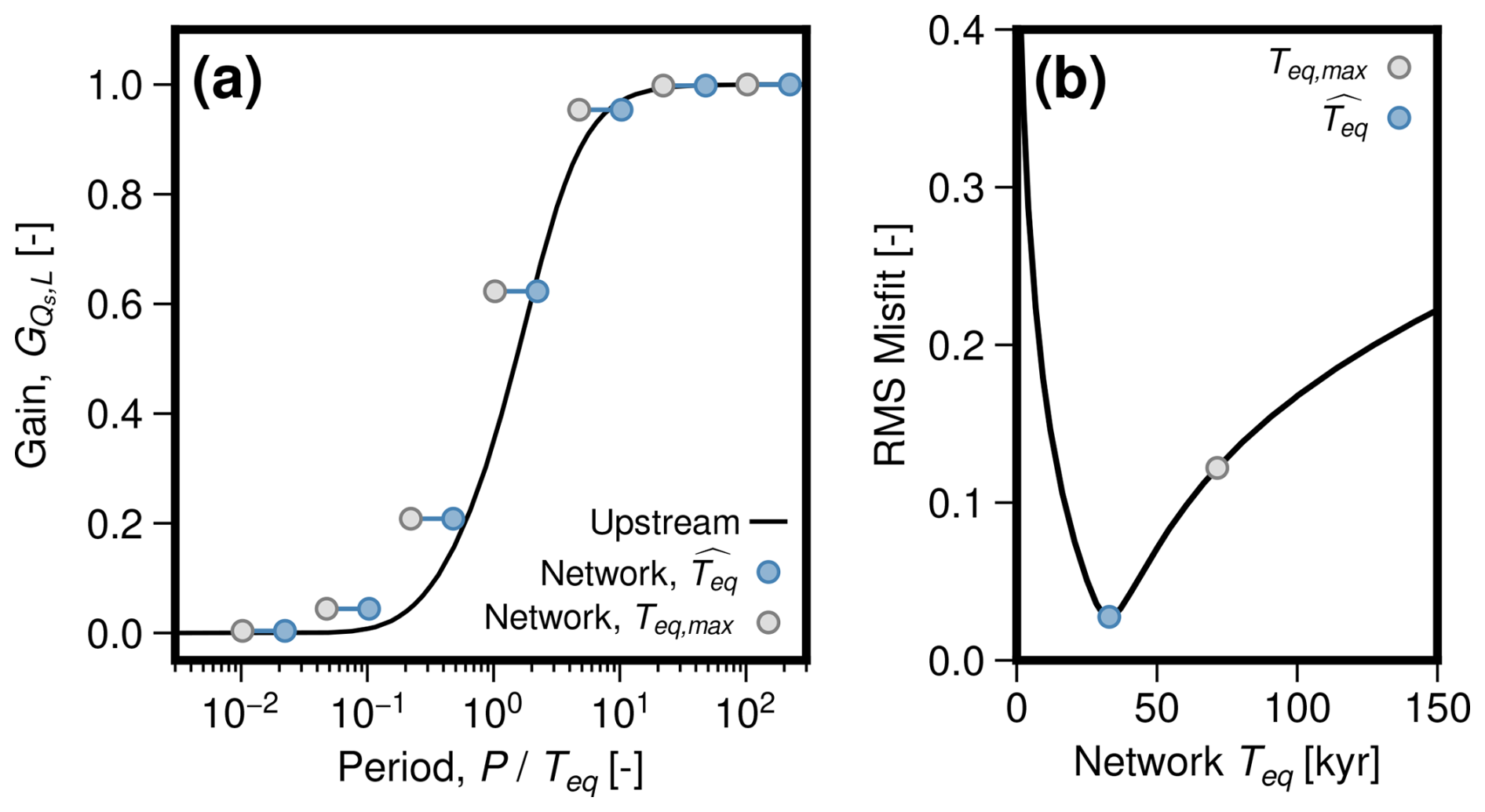
Figure 9 Procedure for calibrating network equilibration times, $\widehat{T_{\text{eq}}}$, by minimising the difference between sediment-discharge gain at the outlet, $G_{Q_{\mathrm{s}},L}$, as a function of normalised forcing period, $P/T_{\text{eq}}$, for a given network and the single-segment, upstream supply case. (a) Black line shows $G_{Q_{\mathrm{s}},L}$ as a function of $P/T_{\text{eq}}$ for the single-segment, upstream supply case, according to analytical solution of McNab et al. (2023). Grey circles show $G_{Q_{\mathrm{s}},L}$ for the network, where T_eq is defined using the network's maximum length. Blue circles show $G_{Q_{\mathrm{s}},L}$ for the network, where T_eq is defined as that which provides the optimal fit to the single-segment, upstream supply case. (b) Black line shows root-mean-square (RMS) misfit between $G_{Q_{\mathrm{s}},L}$ for the network and for the single-segment, upstream supply case, as a function of network T_eq. Grey and blue circles show points corresponding to those shown in (a).

We next consider the full set of network simulations with 40 inlet segments (Fig. 10). When network equilibration time is defined using the networks' maximum lengths, T_eq,max, there is considerable vertical spread in $G_{Q_{\mathrm{s}},L}$ (we used T_eq,max to define the periods at which the simulations were run). At intermediate periods, $G_{Q_{\mathrm{s}},L}$ varies by up to a factor of approximately two between networks at the same forcing period (Fig. 10a–d). This variation in $G_{Q_{\mathrm{s}},L}$ confirms that networks with the same number segments but different geometries respond differently to external forcing. Using $\widehat{T_{\text{eq}}}$, the same measurements of $G_{Q_{\mathrm{s}},L}$ spread out horizontally, closely following the predicted curve (Fig. 10a–d). This horizontal spread corresponds to a range in empirical $\widehat{T_{\text{eq}}}$ between approximately 20–150 kyr, for the cases with uniform segment lengths, which can be attributed to differences in the network topology (see inset histograms in Fig. 10e and g); this range increases to approximately 15–250 kyr for the cases with non-uniform segment lengths (see inset histograms in Fig. 10f and h). We obtain similar results for the set of simulations with numbers of inlet segments ranging between 2 and 150 (Fig. S4 in the Supplement).

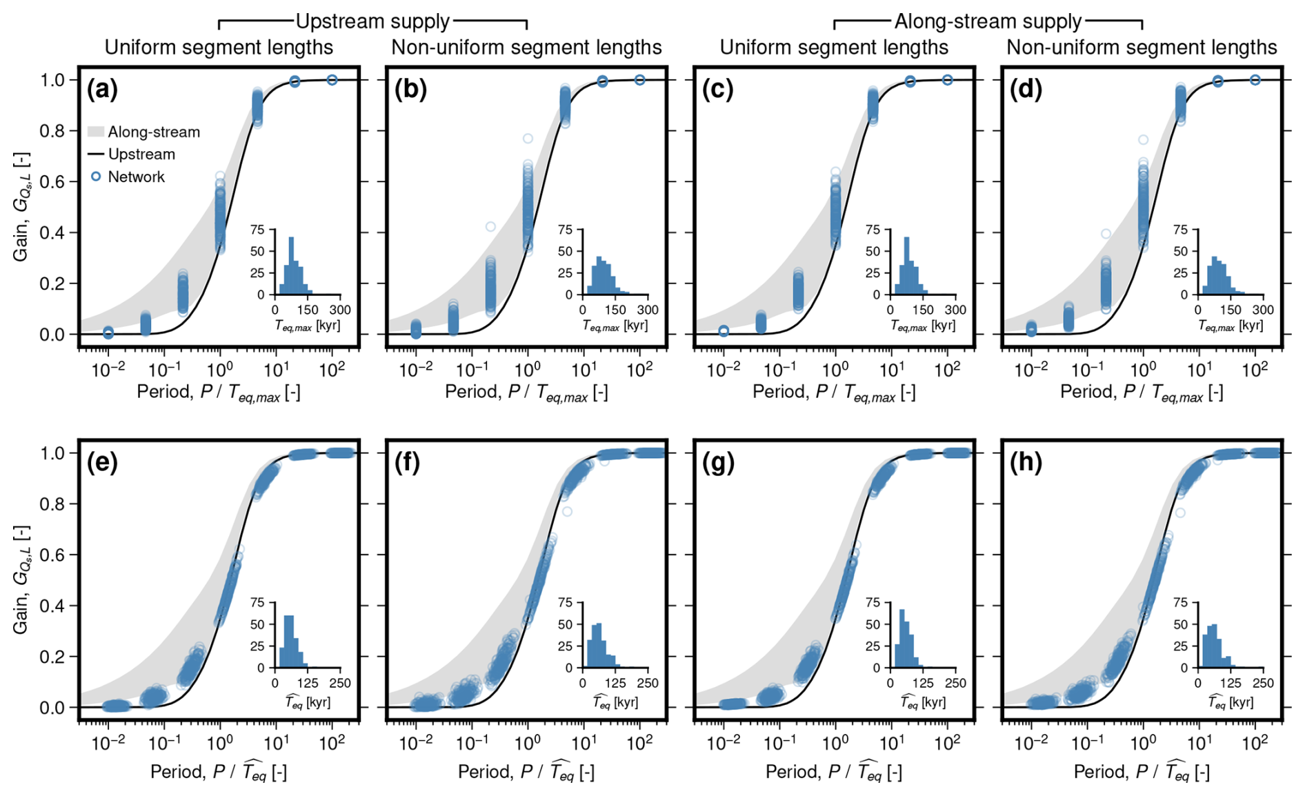
Figure 10 Gain for sediment discharge at the valley outlet, $G_{Q_{\mathrm{s}},L}$, as function of forcing period, P, normalised by equilibration time, T_eq, for the set of networks with number of inlet segments, N₁=40. Circles represent networks, the black line represents the single segment case where all sediment and water are supplied at the inlet (McNab et al., 2023), and the grey band represents range for the single-segment case with along-stream supply of sediment and water, with power-law exponents $p_{x,Q_{\mathrm{w}}}$ and $p_{x,Q_{\mathrm{s}}}$ between 0.8 and 2.4. (a–d) T_eq defined using maximum length (i.e., maximum distance from valley inlet to outlet). (e–h) Empirical $\widehat{T_{\text{eq}}}$ optimised for each network to minimise the difference between $G_{Q_{\mathrm{s}},L}$ as function of $P/T_{\text{eq}}$ of the network and the upstream supply case. Inset histograms show distributions of obtained $\widehat{T_{\text{eq}}}$. (a, e) Uniform segment lengths with no along-stream supply of sediment and water; (b, f) non-uniform segment lengths with no along-stream supply of sediment and water; (c, g) uniform segment lengths with along-stream supply of sediment and water; (d, h) non-uniform segment lengths with along-stream supply of sediment and water. Equivalent results for the set of networks with N₁=2–150 in Fig. S4.

Equilibration times defined empirically in this way are only useful if they are predictable from measurable network properties; only then can they provide insight into the behaviour of natural systems. We therefore compute Spearman's rank correlation coefficients between network effective lengths, $\widehat{L}$, derived from the empirical equilibration times (Eq. 26), and the network properties defined in Sect. 5.2 (Fig. 11; see Figs. S5 and S6 in the Supplement for cross plots of all network metrics against $\widehat{L}$). (We choose Spearman's rank since the functional forms of relationships between network effective lengths and the various network metrics are not known a priori.) For the set of networks with 40 valley inlet segments and uniform segment lengths, we obtain moderate correlations between $\widehat{L}$ and Horton's and Tokunaga's topological metrics (r≈0.4–0.7; Fig. 11a and c). However, apart from for the length ratio R_L, correlations are greatly reduced for the network case with non-uniform segment lengths and for the set with variable numbers of inlet segments (Fig. 11a–d). In general, the series of metrics based on topological and absolute lengths perform significantly better (r>0.6), in particular the average lengths (〈l〉, 〈l_I〉, 〈L〉, 〈L_I〉; r>0.7). The average absolute lengths, 〈L〉 and 〈L_I〉, perform well across all network cases (r>0.99), while the performance of the average topological lengths, 〈l〉 and 〈l_I〉, deteriorates for networks with non-uniform segment lengths (r≈0.7). Relationships between 〈L_I〉 and $\widehat{L}$ for each of the network scenarios are well approximated by linear relationships passing through the origin with gradients of 1.35–1.45 (Fig. 11e–l). We find moderate negative correlations between effective length and topological widths and the inverse Hack exponent, p. In particular, the mean topological width, 〈w〉, performs well for networks with uniform segment lengths ($r\approx -\mathrm{0.8}$), but, as with the topological length metrics, this relationship deteriorates for networks with non-uniform segment lengths. For the set of networks with variable numbers of valley inlet segments, these correlations become positive and decrease in magnitude.

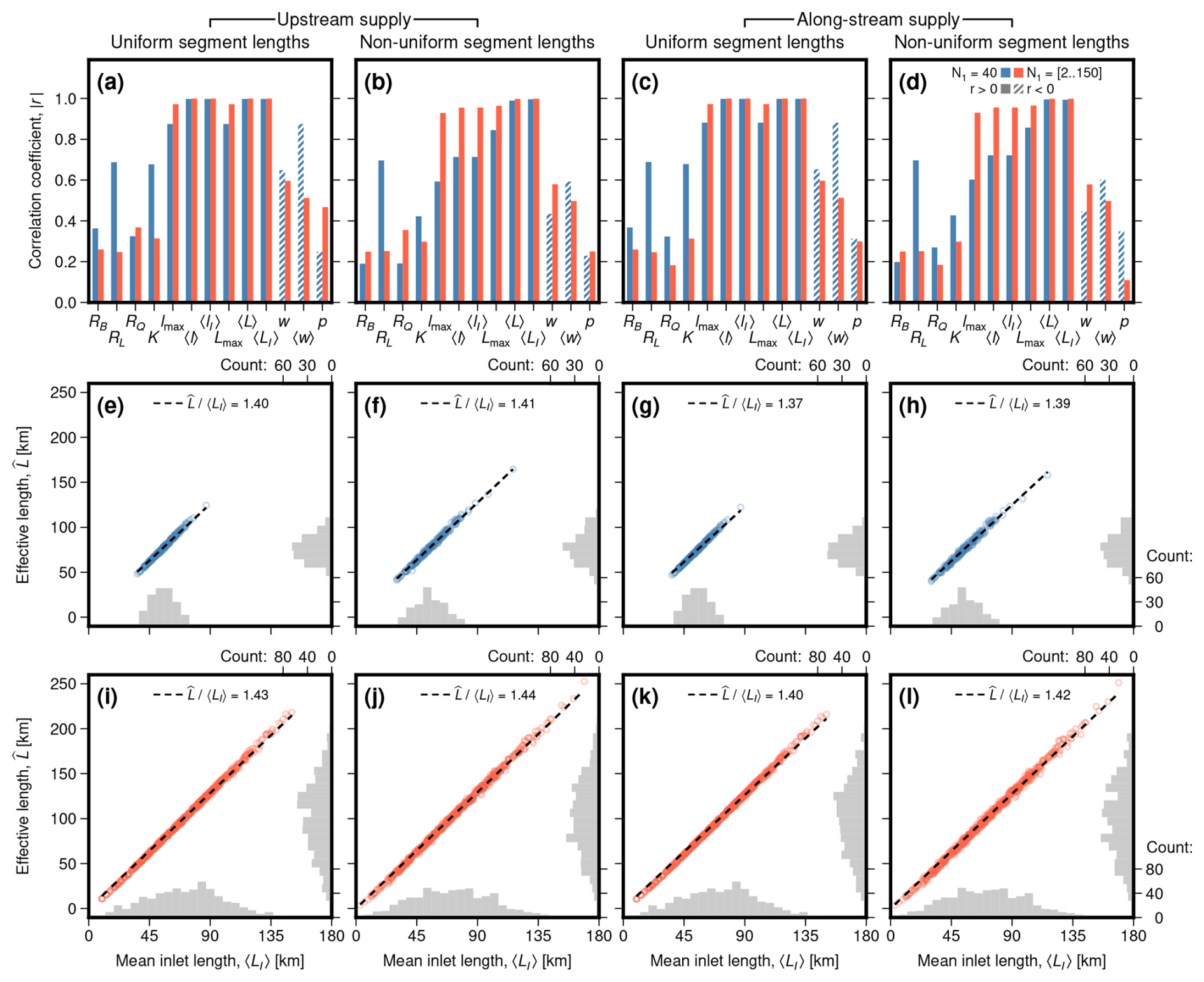
Figure 11 Controls on the network effective length, $\widehat{L}$, for four network scenarios with: (a, e, i) uniform segment lengths with no along-stream supply of sediment and water; (b, f, j) non-uniform segment lengths with no along-stream supply of sediment and water; (c, g, k) uniform segment lengths with along-stream supply of sediment and water; (d, h, l) non-uniform segment lengths with along-stream supply of sediment and water. (a–d) Magnitude of Spearman's rank correlation coefficient, $\left|r\right|$, between $\widehat{L}$ and selected network properties. Blue bars represent sets of 200 networks each with 40 valley inlet segments; orange bars represent sets of 600 networks with 2–150 valley inlet segments. Solid bars correspond to positive trends while hatched bars correspond to negative trends. (e–h) Circles show $\widehat{L}$ as a function of mean length, 〈L_I〉, for each network in the sets of simulations with 40 valley inlet segments. Histograms show distributions of each variable. Dashed lines show best-fit linear relationship, constrained to pass through the origin. (i–l) As (e–h) for the sets of simulations with 2–150 valley inlet segments.

Both the mean length, 〈L〉, and the mean inlet length, 〈L_I〉, predict network effective length equally well. In the remainder of the paper, we focus on 〈L_I〉; it is, to us, more intuitively connected to the length of a single-segment valley. This choice is, nevertheless, arbitrary, and similar arguments to those we make in the following also apply to 〈L〉.

The distributions of $\widehat{L}$ as a function of 〈L_I〉 for the set of networks with 2–150 valley inlet segments are slightly non-linear, implying that the ratio of $\widehat{L}$ to 〈L_I〉 varies with network size (Fig. 11i–l). Indeed, in every scenario, $\widehat{L}/\langle L_{\mathrm{I}}\rangle$ is close to one for small numbers of inlet segments, then increases quickly as the the number of inlets segments increases, until about 50 inlet segments are reached, after which it increases more slowly (Fig. 12). In our simulations, the upstream supply cases reach a maximum value of $\widehat{L}/\langle L_{\mathrm{I}}\rangle \approx \mathrm{1.45}$, while the along-stream supply cases reach a slightly lower maximum of $\widehat{L}/\langle L_{\mathrm{I}}\rangle \approx \mathrm{1.42}$. The scenarios with non-uniform segment lengths (Fig. 12b and d) show considerably more scatter than those with uniform segment lengths (Fig. 12a and c).

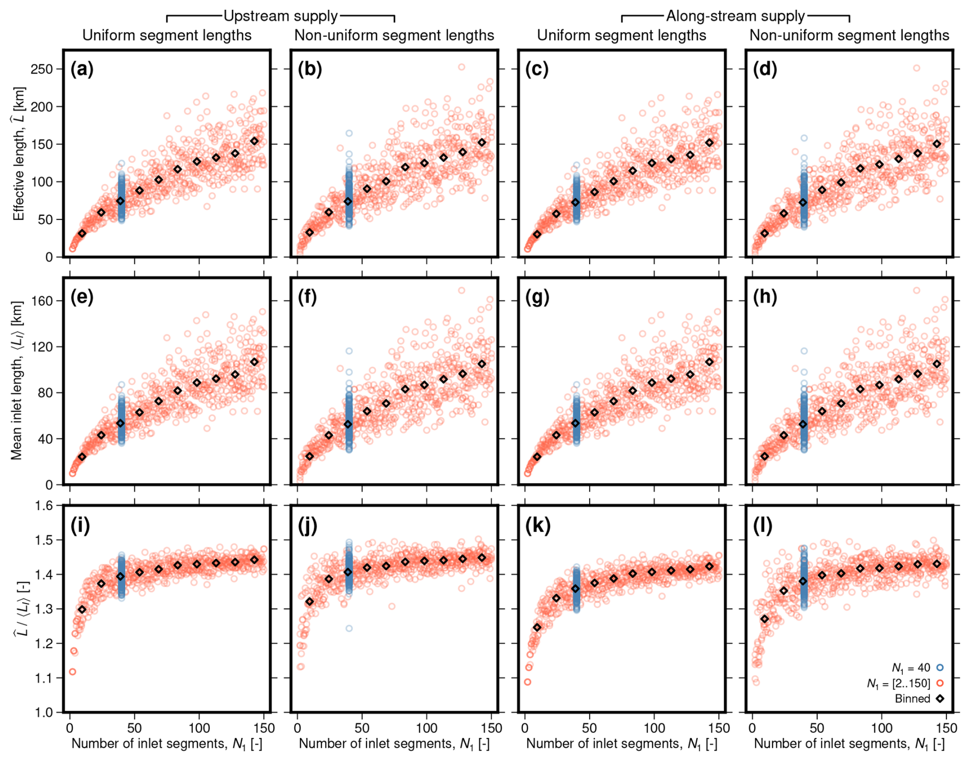
Figure 12 (a–d) Network effective lengths, $\widehat{L}$; (e–h) mean inlet lengths, 〈L_I〉; and (i–l) their ratio as functions of the number of valley inlet segments, N₁, for four network scenarios with: (a, e, i) uniform segment lengths with no along-stream supply of sediment and water; (b, f, j) non-uniform segment lengths with no along-stream supply of sediment and water; (c, g, k) uniform segment lengths with along-stream supply of sediment and water; (d, h, l) non-uniform segment lengths with along-stream supply of sediment and water. Circles represent individual networks; blue belong to set of simulations with N₁ fixed to 40, while orange belong to set with N₁ between 2 and 150. Diamonds represent binned values.

5.4.2 Network response as function of forcing period

Accounting for the effects of networks' structure on their equilibration times allows us to explore their behaviour in more detail within a common reference frame. In the following, we show how gain and lag vary as a function of period, where period is normalised by the networks' individual equilibration times, $\widehat{T_{\text{eq}}}$, determined above (Fig. 13, for results with N₁=40; Fig. S7 in the Supplement for results with N₁=2–150). As with the single-segment cases, we found that elevation gain, G_z, and lag, φ_z, are similar regardless of whether sediment or water supply is varied. Therefore, only the results for variation in sediment supply are shown (Figs. 13a–h and S7a–h); corresponding results for variation in water supply are shown in Figs. S8 and S9 in the Supplement.

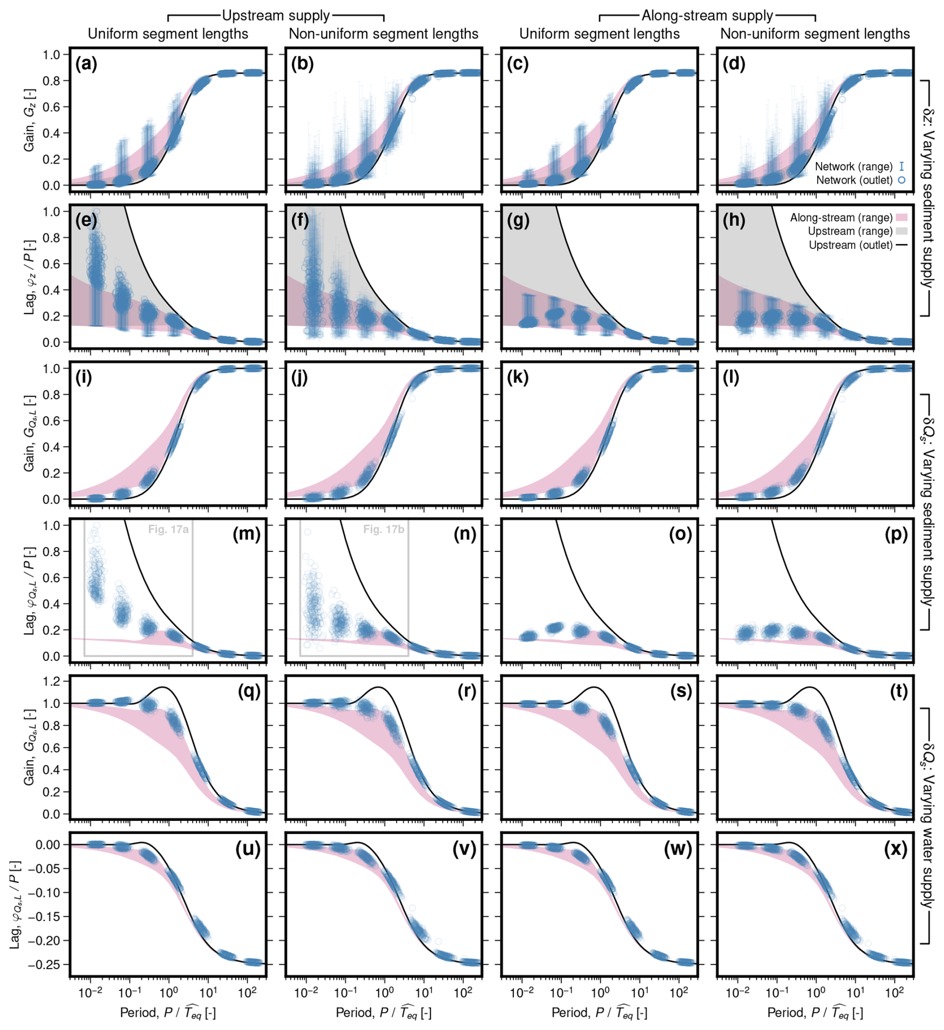
Figure 13 Gain, G, and lag, φ, as functions of forcing period, P, normalised to empirical equilibration time, $\widehat{T_{\text{eq}}}$, for the set of networks with number of inlet segments, N₁=40. Four network scenarios are shown: (a, e, i, m, q, u) uniform segment lengths with no along-stream supply of sediment and water; (b, f, j, n, r, v) non-uniform segment lengths with no along-stream supply of sediment and water; (c, g, k, o, s, w) uniform segment lengths with along-stream supply of sediment and water; (d, h, l, p, t, x) non-uniform segment lengths with along-stream supply of sediment and water. (a–d) Elevation gain, G_z, in response to variation in sediment supply. Circles represent value at the network outlet, where error bars represent range throughout network. Black line and grey band represent value at outlet and range along stream, respectively, for single-segment case with all water and sediment supplied at the inlet (according to analytical solution of McNab et al., 2023). Pink band represents range along stream for single-segment case with along-stream supply of water and sediment, for power-law exponents $p_{x,Q_{\mathrm{w}}}=p_{x,Q_{\mathrm{s}}}=\mathrm{0.8}$–2.4. (e–h) As (a–d) for elevation lag. (i–p) As (a–h) for sediment-discharge gain, $G_{Q_{\mathrm{s}}}$, and lag, ${\mathit{\phi }}_{Q_{\mathrm{s}}}$. Note that only values for the outlet are shown. Panels (i–l) are the same as Fig. 10e–h. (q–x) As (i–p) for response to variation in water supply. Equivalent results for the set of networks with N₁=2–150 are shown in Fig. S7. Equivalent results to panels (a–h) for variation in water supply are shown in Fig. S8, and for the set of networks with N₁=2–150 are shown in Fig. S9.

For each of the network scenarios, G_z, like $G_{Q_{\mathrm{s}},L}$, follows a similar pattern to the single segment cases: it remains close to zero for short forcing periods and increases to approximately $\mathrm{6}/\mathrm{7}$ (≈0.86) as the forcing period increases beyond the equilibration time (Fig. 13a–d). The range in G_z within individual networks is, however, significantly larger than for the single-segment cases. The network scenarios with non-uniform segment lengths (Fig. 13b and d) also show a greater range and variability than those with uniform segment lengths (Fig. 13a and c). ${\mathit{\phi }}_z/P$, as in the single-segment cases, is generally largest for small forcing periods and decreases for longer forcing periods (Fig. 13e–h). This pattern particularly holds for the networks with only upstream supply of sediment and water, for which φ_z typically lies between the single-segment, upstream and along-stream supply cases (Fig. 13e and f; see also Howard, 1982). However, for the network scenarios with along-stream supply of sediment and water, ${\mathit{\phi }}_z/P$ reaches a peak of around 0.2 with $P/\widehat{T_{\text{eq}}}\approx {\mathrm{10}}^{-\mathrm{1}}$, and then begins to decrease slightly for shorter periods (Fig. 13g and h). There, the along-stream range in φ_z is also considerably lower than for networks without along-stream supply of sediment and water. We obtained similar patterns for single-segment cases with along-stream supply of sediment and water (Fig. 7d).

When sediment supply is varied, sediment-discharge gain, $G_{Q_{\mathrm{s}}}$, and lag, ${\mathit{\phi }}_{Q_{\mathrm{s}}}$, at the valley outlet vary in similar ways to those described for G_z and φ_z above (Fig. 13i–p). However, as in the single-segment cases, different patterns arise when water supply is varied (Fig. 13q–x). There, $G_{Q_{\mathrm{s}},L}$ is approximately one for short forcing periods, and drops to zero for long forcing periods. Unlike the single-segment, upstream supply case, but similar to the single segment, along-stream supply case, there is no significant amplification ($G_{Q_{\mathrm{s}},L}>\mathrm{1}$) at intermediate periods. ${\mathit{\phi }}_{Q_{\mathrm{s}},L}$, again similar to the single segment cases, is zero for short forcing periods and drops to −0.25 for long forcing periods.

5.4.3 Spatial patterns of aggradation and incision

Patterns of aggradation and incision vary spatially within networks, in ways that depend on network geometry and could influence the distribution and timing of terrace formation (Figs. 14–16). We first illustrate how gain and lag vary spatially, as well as corresponding elevation time series for selected segments, for an example network simulation with forcing period equal to its empirical equilibration time, $\widehat{T_{\text{eq}}}$ (Fig. 14). We then show gain and lag as functions of downstream distance, for all four cases of the same network topology and a range of forcing periods (Fig. 15; to aid visualisation, we also provide a Video Supplement showing corresponding patterns of aggradation and incision in plan view). Finally, we show how these patterns vary for different network topologies, distributed from most compact to most elongate (Fig. 16). It is impractical to show here results from each of the 796 networks we tested; we do, however, provide a script in the accompanying software repository allowing interested readers to plot the entire dataset (McNab, 2025). Although, in detail, spatial patterns of aggradation and incision are unique to each individual network, some general features can be identified, of which the examples in Figs. 14–16 are representative.

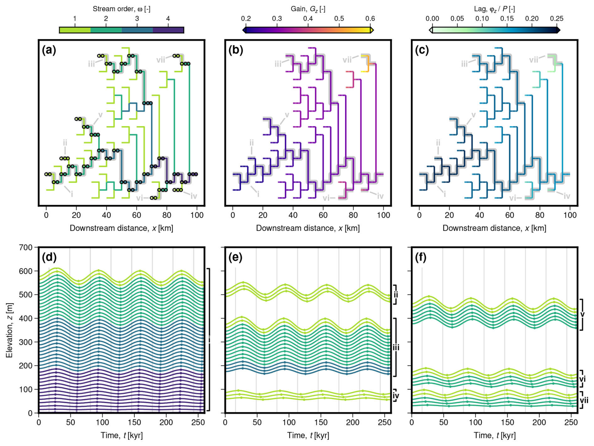
Figure 14 Spatial variation of gain, G_z, and lag, ${\mathit{\phi }}_z/P$, within a network with uniform segment lengths and no along-stream supply of sediment and water, when sediment supply is varied with a period, P, equal to the network's empirically obtained equilibration time, $\widehat{T_{\text{eq}}}$. (a) Schematic network planform shaded by stream order. Thicker grey lines highlight streams, while circles show positions of specific nodes, whose evolution are shown in (d–f). (a) As (a) shaded by G_z. (c) As (a) shaded by ${\mathit{\phi }}_z/P$. (d) Elevation, z, as a function of time, t, for selected nodes along stream (i), as shown in (a–c). Grey lines show timing of peaks and troughs in the imposed forcing; circles show peaks and troughs in elevation. Colours indicate stream order. (e) As (d) for tributary streams (ii–iv). (f) As (d) for tributary streams (v–vii).

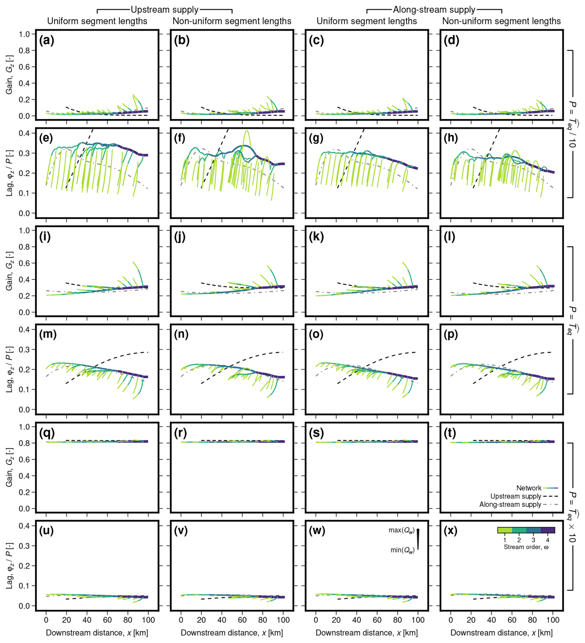
Figure 15 Gain, G_z, and lag, ${\mathit{\phi }}_z/P$, as functions of downstream distance for three forcing periods and networks with: (a, e, i, m, q, u) uniform and (b, f, j, n, r, v) non-uniform segment lengths and upstream supply of sediment and water; (c, g, k, o, s, w) uniform and (d, h, l, p, t, x) non-uniform segment lengths with along-stream supply of sediment and water. (a–d) G_z as function of downstream distance where $P=\widehat{T_{\text{eq}}}/\mathrm{10}$. Solid lines show network segments shaded by stream order, with line thickness scaled by water discharge (see key in panel w). Black dashed line shows single-segment case where all sediment and water is supplied at the valley inlet, with length equal to the network empirical effective length, $\widehat{L}$ (according to analytical solution of McNab et al., 2023). Grey dashed/dotted line shows single-segment, along-stream supply case, with power-law exponent equal to the network's best-fitting exponent, and with length equal to the network's maximum length. (e–h) As (a–d) for φ_z. (i–p) As (a–h) for $P=\widehat{T_{\text{eq}}}$. (q–x) As (a–h) for $P=\widehat{T_{\text{eq}}}\times \mathrm{10}$.

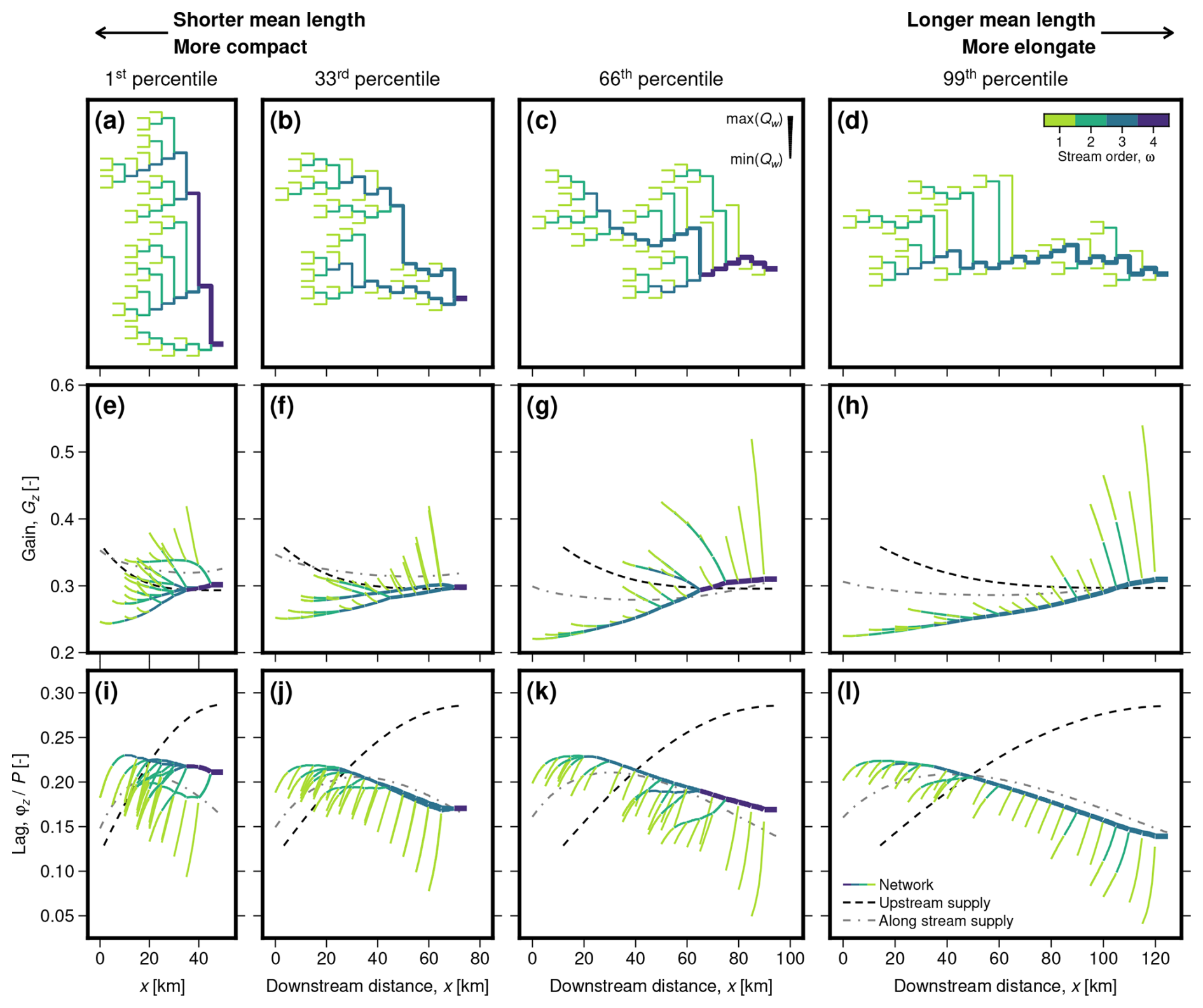
Figure 16 Gain, G_z, and lag, ${\mathit{\phi }}_z/P$, as functions of downstream distance for networks with a range of mean lengths. From the set of networks with number of inlet segments, N₁=40, we select networks with mean lengths corresponding to the 1st (i.e., shortest) percentile (a, e, i), 33rd percentile (b, f, j), 66th percentile (c, g, k), and 99th (i.e., longest) percentile (d, h, l). (a–d) Schematic network planforms, where colour indicates stream order, and line thickness is scaled by water discharge (see key in c). (e–h) G_z as function of downstream distance. Solid lines show network segments shaded by stream order, with line thickness scaled by water discharge (see key in panel c). Black dashed line shows single-segment, upstream supply case, with length equal to the network empirical effective length, $\widehat{L}$ (according to analytical solution of McNab et al., 2023). Grey dashed/dotted line shows single-segment, along-stream supply case where sediment and water follow power law with exponent equal to the network's best-fitting exponent, and with length equal to the network's maximum length. (i–l) As (a–d) for φ_z.

G_z is broadly lowest upstream and highest downstream in the network. It steadily increases downstream along the higher order segments (in the example here, ω>2), similar to patterns in mid- and down-stream sections of the single-segment case with along-stream supply of sediment and water (Figs. 6b and Fig. 15a–d, i–l, q–t). However, on lower order streams (here ω≤2), G_z is generally highest at the inlet and decreases downstream, similar to the simple single-segment case with all sediment and water supplied at the inlet, and to the uppermost sections of the single-segment case with continuous supply of sediment and water along stream. G_z is generally highest at the inlet of tributaries that meet higher order segments near the network's downstream end. This pattern holds also for short forcing periods ($P\approx T_{\text{eq}}/\mathrm{10}$), where, while amplitudes of aggradation and incision approach zero along higher order segments, appreciable amplitudes remain on some lower order segments (Fig. 15a–d).

φ_z is broadly highest upstream and lowest downstream in the network. It steadily decreases downstream along the higher order segments; this decrease is more gradual than the increase in φ_z downstream that arises in the single-segment, upstream supply case, so that the network response appears more uniform along stream (Figs. 14c and Fig. 15e–h, m–p, u–x; see also Howard, 1982). This pattern is similar to that we obtained in mid- and down-stream sections of the single segment, along-stream supply case (Fig. 6d and e). However, on lower order segments, φ_z is generally lowest at the inlet and increases downstream, similar to the single-segment, upstream supply case, and to the uppermost sections of the single-segment, along-stream supply case (Figs. 6d and e, 14d, and 15e–h, m–p, u–x). This increase in φ_z downstream occurs more rapidly for shorter forcing periods (compare Fig. 15e–h, for $P=T_{\text{eq}}/\mathrm{10}$ with Fig. 15m–o, for P=T_eq). As such, φ_z is generally lowest at the inlets of, and increases most rapidly along, lower order segments that meet higher order segments near the valley outlet. For the network scenarios with non-uniform segment lengths, these patterns hold for short, lower order segments, but for longer ones, φ_z first increases downstream, before reaching a peak and decreasing downstream before meeting higher order segments (e.g., Fig. 15f and h).

Comparing networks with different geometries, these patterns are most straightforwardly expressed for more elongate networks, which contain a single higher order main stream fed by short lower order streams (Fig. 16d, h, and l). As networks become more compact, middle order streams arise with behaviour intermediate between the lower order and higher order end members (Fig. 16a–c, e–g, i–k). This range of behaviour leads to more complex patterns of aggradation and incision that depend on specific network geometry.

5.5 Interpretation

As in the single-segment case, network responses to variation in sediment and water supply can be understood in terms of the relative timescales of the forcing and network aggradation and incision (e.g., Howard, 1982; Paola et al., 1992; Braun, 2022), and of signal propagation through the network (Figs. 10–16). In both network cases, signal is now introduced at multiple valley inlets, while, in the along-stream supply case, signal is also introduced internally along each network segment. On individual segments, variation in sediment and water delivery from upstream segments transmits signal downstream, while aggradation and incision of downstream segments drives local base-level variation and transmits signal upstream. As in the single-segment, along-stream supply case, accumulation of water downstream means that diffusivity, and the capacity for segments to adjust to external forcing, is greater in downstream, higher order parts of the network.

It is well understood that, in the single-segment case, the timescale over which a diffusive system evolves is set by the square of its length (e.g., Paola et al., 1992; McNab et al., 2023). In the network case, signal is introduced at range of distances from, and therefore must propagate a range of distances to, the network outlet. Our results suggest that the timescale over which a network can aggrade and incise is controlled by the average of these distances (in our terminology, the mean inlet length, 〈L_I〉; Figs. 10–12). This result may also be related to that of Jarvis and Werritty (1975), who showed that metrics related to a network's mean length retain more information about network structure than those focused on branching statistics (i.e., Horton's and Tokunaga's laws) or the accumulation of drainage area and water discharge (i.e., Hack's law). For example, two networks can have the same maximum length but very different distributions of segments; the mean length, in contrast, takes into account the entire network structure.

This framework also helps make sense of spatial variation in the network response (Figs. 14–16). On lower order streams, the response is dominated by signal propagating from upstream inlets: G_z therefore generally decreases and φ_z generally increases downstream. Higher order streams, in contrast, are influenced by signal propagating from a range of distances up- and down-stream, as well as, in the along-stream supply case, local signal sources. Signals introduced far upstream take time to propagate to high order segments and lose amplitude as they do so. However, signals introduced on short tributaries can propagate efficiently to higher order streams, behaving similarly to the local sources of the single-segment along-stream supply case. Combined with increased diffusivity on higher order segments, these effects result in a general increase in G_z and decrease in φ_z along higher order segments, similar to single-segment, along-stream supply case (this general reduction of φ_z on high order segments, such that the network response is more spatially uniform than the single-segment, upstream supply case, was also noted by Howard, 1982). Higher amplitudes and lower lags on higher order segments also feed back to short adjacent tributaries by varying their base level. Thus, G_z is maximised and φ_z minimised on short tributaries close to the valley outlet.

The networks with upstream and along-stream supply of sediment and water behave similarly in many respects. In particular, we obtained very similar estimates of equilibration times and effective lengths for the two cases, with those of the along-stream supply networks being only slightly shorter (Figs. 11 and 12). These patterns likely reflect the fact that, even when along-stream supply is included, an increasing fraction of a segment's sediment supply is still derived from upstream as the segment order increases. Thus, for higher order segments such as the outlet, whose behaviour we used to estimate $\widehat{T_{\text{eq}}}$, the signal propagating from upstream dominates in both cases. An exception arises in patterns of φ_z,L, for both variation and sediment and water supply, and ${\mathit{\phi }}_{Q_{\mathrm{s}},L}$, for variation in sediment supply, at low forcing periods (i.e., $P\lesssim \widehat{T_{\text{eq}}}$; Fig. 13e–f, m–n). Here, signals propagating from upstream are strongly damped, so that, in the along-stream supply case, local sources begin to dominate, and φ_z,L and ${\mathit{\phi }}_{Q_{\mathrm{s}},L}$ even decrease with decreasing period (similar to the single-segment, along-stream supply case; Fig. 7d and e). In contrast, in the upstream supply case, lag times at the network outlet strongly diverge as $P/\widehat{T_{\text{eq}}}$, decreases, so that a wide range of ${\mathit{\phi }}_z/P$ and ${\mathit{\phi }}_{Q_{\mathrm{s}}}/P$ occurs even for simulations with similar $P/\widehat{T_{\text{eq}}}$.

This last result suggests that, for the upstream supply networks, the mean inlet length is not a good predictor of lag time at the outlet for short forcing periods. If progressive damping of signals as they propagate downstream results in inlets positioned far upstream having increasingly limited influence on aggradation and incision at the outlet, a corollary is that inlets close to the outlet should exert greater influence. Indeed, distinguishing networks by the distance upstream from the outlet to their closest inlet segment reveals a clear pattern (Fig. 17). For the networks with uniform segment lengths, three populations exist, in which the first inlet occurs two, three or four segments upstream from the outlet; lag times increase as the distance to the first inlet increases (Fig. 17a). For the networks with non-uniform segment lengths, there is more scatter, but the same general pattern is present (Fig. 17b). This scatter may arise due to differences in the distribution of water discharge, and hence diffusivity, along the paths from the first inlet downstream to the outlet. In the networks with uniform segment lengths, water discharge increases downstream at consistent intervals, so that networks with equal distances to the first inlet also have similar distributions of discharge along the path. Conversely, in the networks with non-uniform segment lengths, discharge and distance are decoupled, so that two networks with similar distances from the outlet to the first inlet can have very different distributions of discharge along the path, and hence very different rates of signal propagation. These results confirm that, at short forcing periods, aggradation and incision, and, consequently, sediment export, at the network outlet are mainly influenced by network structure close to the outlet. Similarly, we expect the response to short period external forcing at different points within the network to be mainly controlled by local network structures.

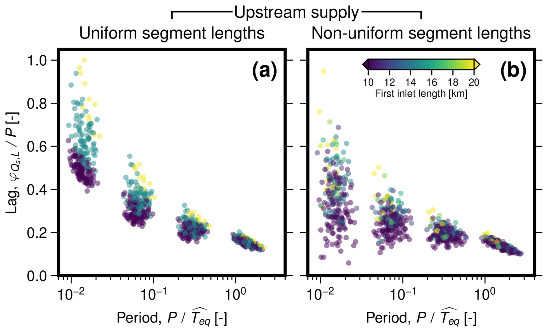
Figure 17 Sediment-discharge lag at the network outlet, ${\mathit{\phi }}_{Q_{\mathrm{s},L}}$, as a function of forcing period, P, normalised by empirical equilibration time, $\widehat{T_{\text{eq}}}$, with focus on shorter forcing periods (see boxes on Fig. 13 for position within wider parameter space). Lag measurements for each network are shaded by distance upstream to the first inlet segment. (a) Networks with only upstream supply and uniform segment lengths. Uniform segment lengths result in three populations in which the first inlet segment occurs two, three or four segments upstream from the outlet. (b) Networks with only upstream supply and non-uniform segment lengths.

6 Discussion

6.1 Single-segment models can predict integrated network behaviour

We have shown that simplified, single-segment models with only upstream supply of sediment and water can accurately predict amplitudes of variation in sediment export from networks with varying complexity, provided an appropriate lengthscale is chosen to characterize the network (Figs. 9–12). We also showed that an appropriate lengthscale for a given network is predictable from its mean inlet length. As such, we propose a modified definition of alluvial river equilibration time appropriate for networks:

$$\begin{array}{}\text{(27)}& T_{\text{eq}}={\displaystyle \frac{{\widehat{L}}^{\mathrm{2}}}{\langle \mathit{\kappa }\rangle }}\approx {\displaystyle \frac{{k_L}^{\mathrm{2}}\langle L_{\mathrm{I}}{\rangle }^{\mathrm{2}}}{\langle \mathit{\kappa }\rangle }},\end{array}$$

where k_L is a coefficient scaling mean inlet length, 〈L_I〉, to effective length, $\widehat{L}$. The value of k_L depends on the number of network segments and on how discharge varies throughout the network. In our simulations, it increased from close to one for networks with few segments to approximately 1.4–1.45 for networks with many segments (Fig. 12). It may continue to rise slowly for larger networks than those tested here.

This result implies that, if our main concern is the amplitude of variation in sediment discharge at the network outlet (e.g., for studies of downstream stratigraphic records), we can use simplified single-segment models, and avoid the complexity and computational cost of network implementations. We note that, for variation in sediment supply, single-segment models with only upstream supply of sediment and water do not predict network lag times as effectively as their amplitudes (Fig. 13e–f, m–n). When sediment supply is varied at relatively short forcing periods (P<T_eq), lag times for networks with only upstream supply are lower than predicted by the single-segment case and considerable scatter is introduced. We found that this pattern reflects a decoupling of aggradation and incision at the outlet from distant parts of the network, and a greater influence of network structure close to the outlet, such as the distance from the outlet to its closest inlet (Fig. 17). Such nuances are not captured by single-segment models. For networks with along-stream supply of sediment and water, lag times follow the single-segment, along-stream supply case more closely than the single-segment, upstream supply case across the range of forcing periods we tested. We also stress that, in all our simulations, we varied sediment and water supply uniformly across the network. In reality, forcing could occur more locally, for example if a large landslide delivers excess sediment to a specific tributary, or if orographic effects influence precipitation patterns across a catchment. Such localised forcing may affect sediment discharge at the outlet in different ways from the simulations shown here, depending, for example, on the distance from the outlet at which the forcing occurs.

Howard (1982), analysing a single example network configuration, also noted a broad similarity between its behaviour and that of a single-segment model. Comparing a single-segment model with a network of equal maximum length and equal water discharge at the outlet, he estimated the response time to be approximately six times longer in the network, based on the time needed to approach equilibrium following a step change in the hydraulic regime. This result may appear to conflict with our analysis, in which network equilibration times are typically similar to or shorter than single-segment models with the same maximum length (Figs. 9 and 10a–d). The difference, however, arises due our different treatments of water discharge. Rather than comparing networks and single-segment models with equal maximum discharge, we used mean discharge in our definitions of network effective length and equilibration time (Eqs. 26 and 27). In our set of networks with forty inlet segments, maximum discharge was on average six times larger than mean discharge, decreasing our estimated equilibration times by an average factor of around six relative to Howard (1982). Meanwhile, Howard (1982)'s network has 39 inlet segments, a maximum topological length of 30, and a mean inlet topological length of around 18; in this case, the network maximum length provides a reasonable approximation of its effective length (too long by a factor of ≈1.15). Thus, our estimates of network equilibration time are broadly consistent with that of Howard (1982).

What controls a network's mean inlet length? In our simulations, we constructed networks with specified numbers of segments and specified (average) segment lengths, approximately corresponding to a consistent drainage area. In such network populations, the shortest mean lengths occur in the most compact networks, while the longest mean lengths occur in the most elongate (Fig. 16). However, in nature, spatial constraints such as coastlines or fault-bounded mountain ranges may be more relevant, and could instead fix a network's main stream or maximum length. Comparing networks with equal main stream lengths, the relationship is reversed: the shortest mean lengths occur in the most elongate networks, which will also have smaller drainage areas, while the longest mean lengths occur in the broadest networks. Robinson and Scheingross (2024) argued that, while tributaries tend to be arranged in a regular fashion in tectonically quiescent areas, this pattern can be disrupted by faulting in tectonically active areas. This result implies that network structures in tectonically active regions can be particularly irregular, which could lead to a wide range of mean lengths, equilibration times, and responses to external forcing in adjacent catchments of similar sizes. Yi et al. (2018) also showed that basins tend to be more elongate in more arid regions. Depending on whether networks of similar drainage areas or similar main stream lengths are compared, this effect could introduce a tendency towards longer network mean lengths and response times, or shorter mean lengths and response times, respectively. These patterns may therefore exacerbate or counteract to some extent the effect of reduced water discharge on the response time of alluvial networks in arid regions (Eq. 12; e.g. McNab et al., 2023).

6.2 Detailed network behaviour is complex and network dependent

Although networks' integrated responses to external forcing, as expressed in variations in sediment discharge at their outlets, appear to be predictable using simplified, single-segment models, patterns of aggradation and incision within them show considerable complexity (Figs. 14–16). Specifically, amplitudes of aggradation and incision (G_z) and the extent to which they lag behind the imposed forcing (φ_z) vary along stream and between streams of different orders. This complexity arises despite relatively simple, spatially uniform, sinusoidal variations in sediment and water supply, as a consequence of the dynamics of signal propagation in networks (in contrast to the relatively simple, unidirectional signal propagation associated with single-segment models). Complex distributions of terraces and their ages in natural networks therefore need not imply complex and local variations in sediment and water supply. In detail, patterns of G_z and φ_z throughout a specific network depend on its specific structure. We therefore argue that, if a detailed understanding of dynamics of aggradation and incision in a specific network are desirable – for example, to aid interpretation of terrace ages or geometries – then that specific network should be modelled using approaches like the one we employ here. Nevertheless, there are some general features in patterns of G_z and φ_z that appear to be common to most networks and have implications for the distribution and timing of terrace formation.

G_z describes variations in the amplitude of aggradation and incision, relative to imposed variations in sediment and water supply, which in turn influence the likelihood of terrace formation and preservation; higher amplitudes of aggradation and incision are more likely to result in long lived terrace sequences (Figs. 14b, d–f and 15a–d, i–p, q–t). Note that, to obtain absolute amplitudes of aggradation and incision, G_z is multiplied by steady state elevation (Eq. 15), so that it modulates a general tendency towards higher amplitudes at greater distances from the outlet (McNab et al., 2023). G_z is generally higher closer to the network outlet, canceling out to some extent the natural tendency for amplitudes of aggradation and incision to decrease towards the outlet, and thus promoting terrace formation further downstream. On lower order segments that join higher order segments near the outlet, G_z decreases rapidly downstream, so that amplitudes of aggradation and incision decrease particularly quickly (Figs. 14e and f and 15a–d). On such tributaries, terrace formation is therefore more likely than on adjacent higher order segments, but this likelihood decreases quickly away from valley inlets towards higher order segments. Appreciable amplitudes of aggradation and incision (G_z≈0.2) persist on such segments even for short forcing periods, suggesting that terrace formation is possible in specific parts of a network even when the timescales of variation in sediment or water supply are much shorter than its equilibration time ($P\approx T_{\text{eq}}/\mathrm{10}$; Fig. 15a–d).

Network φ_z is typically lower and more uniform along stream, particularly along higher order segments, compared to the simple unidirectional signal propagation predicted for the single-segment, upstream supply case (as noted by Howard, 1982). Nevertheless, φ_z can vary spatially by factors of 2–3 in simulations with significant amplitudes of aggradation and incision (e.g., with P≈T_eq; Figs. 15m–p and 14i–l), implying that terrace formation can occur diachronously throughout a network, and result in a single terrace surface whose age varies spatially despite a simple, spatially uniform forcing (Figs. 14c, d–f and 15e–h, m–p, u–x). On higher order segments, φ_z generally increases upstream, so that terrace formation will occur progressively later away from the network outlet. This pattern may superficially resemble upstream propagation of a signal introduced at the valley outlet (i.e., base-level variations), despite being driven by variation in sediment and water supply evenly distributed across the network and its inlets. It arises because signal can arrive at higher order segments relatively efficiently along short tributaries; high order segments that can then, due to their larger discharges and diffusivities, adjust most efficiently. On lower order segments, φ_z generally increases away from valley inlets, so that terrace formation will appear to propagate downstream. This effect is particularly pronounced on lower order segments that join higher order segments close to the network outlet, where φ_z can increase rapidly downstream and could generate a wide range of terrace ages over a relatively short distance (Figs. 14e and f and 15e–h, m–p). This pattern arises because these low-order segments experience both direct forcing at their upstream ends, as well as significant variation in local base level associated with the efficient aggradation and incision of higher order segments at their downstream ends.

6.3 Variation in valley width

Throughout our analysis thus far, we have treated valley width, B, as a constant. In natural alluvial valley networks, it can vary both in time and space. That valley widths evolve through time is clear from the preservation of paired terrace sequences, which necessarily record valley narrowing over time (e.g., Tofelde et al., 2022). Models describing the lateral evolution of alluvial valleys have been developed, and could in future be coupled with our network implementation of the long profile model of Wickert and Schildgen (2019) to explore the effects of such behaviour (e.g., Hancock and Anderson, 2002; Turowski et al., 2025).

Several studies have also explored how valley width varies along stream, and in particular as a function of upstream drainage area (e.g., Snyder et al., 2003; Brocard and van der Beek, 2006; Beeson et al., 2018; Clubb et al., 2022). Such measurements can contain significant noise, with considerable short wavelength variation, but typically take a power-law form on average. Turowski et al. (2024) combined a compilation of observed power-law parameters with theoretical arguments to conclude that plausible power-law exponents are in the range 0.03–0.9, with a likeliest value around 0.4–0.5. This broad range suggests that valley width can remain essentially constant downstream, or increase almost as quickly as upstream drainage area (and, by extension, water discharge). Our preceding analysis therefore represents one end member of along-stream valley-width behaviour. To explore the other end member, we ran a second set of simulations in which valley width increased downstream at the same rate as water discharge. This formulation is mathematically convenient because the increasing valley width cancels out the effects of increasing water discharge on the efficiency of sediment transport, so that the diffusivity becomes constant across the network (Eq. 12).

The majority of results for this non-uniform valley width case are very similar to those for the uniform valley width case (see Figs. S10–S15 in the Supplement for single-segment results and Figs. S16–S28 in the Supplement for network results). Again, amplitudes of variation in sediment discharge at the network outlet ($G_{Q_{\mathrm{s}}}$) are well approximated by analytical predictions for the single-segment, upstream supply case (Fig. S16). Effective lengths obtained for the non-uniform valley width case also correlate closely with network mean length (Fig. S18–S20). Ratios of effective length to mean length, k_L, are lower than in the uniform valley width case (up to 1.16 for upstream supply cases and 1.13 for along-stream supply cases; Fig. S21).

Some differences between the uniform and non-uniform valley width cases do arise, because, in the former, diffusivity increases downstream as water accumulates, whereas in the latter, diffusivity is spatially constant. In the uniform valley width case, signal propagation is relatively inefficient upstream or on lower order segments where discharge is low, whereas it is more efficient downstream or on higher order segments with larger discharge. This pattern contributes to a general increase in G_z and decrease in φ_z towards the network outlet. In contrast, in the non-uniform valley width case, signal propagation is equally efficient throughout the network, so that signal propagating from upstream valley inlets has more influence farther downstream, and distributions of G_z and φ_z are more symmetrical along stream. In the single-segment, along-stream supply case, minima in gain and maxima in lag occur further downstream than in equivalent models with uniform valley width (Figs. S12 and S13). In the network case, G_z and φ_z are more uniform along higher order segments, and differences between lower order segments near the outlet and those further upstream are less pronounced (Figs. S26–S27).

This analysis accounts for the effects of smoothly varying valley widths, likely to be representative of alluvial valley networks on average. However, significant local variability can arise, due to, for example, lithological variations, distributions of tectonic structures such as active faults, or geologically recent drainage integration, so that natural networks can contain anomalously narrow or wide reaches (e.g., Hilgendorf et al., 2020; Clubb et al., 2023). Very narrow sections will efficiently transmit signals up- and down-stream, increasing response amplitudes and decreasing response lag times in surrounding parts of the network. Meanwhile, very wide sections will adjust slowly and, depending on the timescale, could act as local points of fixed elevation, decoupling upstream sections from the rest of the network. How such dynamics play out in nature needs to be assessed on a network-by-network basis.

6.4 Choice of network generator

We used a relatively simple approach for randomly generating networks (Shreve, 1966, 1969, 1974). Although this approach theoretically samples all possible binary trees, the number of possible networks far exceeds the number we can practically analyse, such that the network populations we obtained are necessarily incomplete. End-member configurations such as perfect binary trees (in which every internal segment has two internal segments upstream, until a final level of inlet segments) are very unlikely to be selected. Statistics of network populations generated in this way also likely diverge, at least to some extent, from those of natural network populations, since, for example, the networks are not required to be space filling (Abrahams, 1984; Dodds and Rothman, 2000). The high fidelity of the relationship we obtained between network equilibration times and their mean inlet lengths strongly suggests that it will apply to branching networks more generally (Fig. 11). Nevertheless, the statistical results we obtained, such as precise values of the coefficient k_L scaling network mean length to effective length (Eq. 27; Fig. 11), and their variation with network size (Fig. 12), likely depend at least to some extent on our choice of network generator. We also note that, since we did not sample the full range of possible network configurations, we may not have observed the full range of possible behaviour in, for example, spatial patterns of aggradation and incision, or lag at the network outlet (Figs. 15–17). Repeating our analysis using more involved approaches to network generation that appear to produce more naturalistic network populations, such as random walks on lattices (Leopold and Langbein, 1962; Scheidegger, 1967) or Optimal Channel Networks (Howard, 1990; Rodriíguez-Iturbe et al., 1992), or indeed using network populations extracted from real landscapes, may provide results more representative of natural alluvial river systems. Approaches that allow random network populations to be generated with prescribed statistical properties may also facilitate more detailed and systematic exploration of structural controls on network behaviour (Veitzer and Gupta, 2000). In the meantime, these issues highlight the importance of modelling the specific structures of specific networks of interest, particularly when an understanding of spatial patterns of aggradation and incision is required.

6.5 High frequency fluctuations in sediment transport and signal “shredding”

Lastly, we note a superficial similarity between the reduced amplitude of sediment-supply signals we observe at short forcing periods (i.e., G_z, $G_{Q_{\mathrm{s}},L}<\mathrm{6}/\mathrm{7}$ for P≲T_eq) and the concept of signal “shredding”, as proposed by Jerolmack and Paola (2010). This concept builds from the observation that sediment transport in many environments is a threshold process subject to large, autogenic, stochastic fluctuations. Jerolmack and Paola (2010) demonstrated that, if an external signal is imposed with a timescale similar to or shorter than the timescales of these internal fluctuations, it will be smeared across a range of timescales and, consequently, its amplitude will be severely reduced. The original signal is therefore unreconisable in time series of sediment discharge (i.e., it will be “shredded”). This process is distinct from the diffusive damping or buffering we observe, in which signal amplitudes are reduced but their frequency content is preserved (see also Howard, 1982; Paola et al., 1992; Armitage et al., 2013; Goldberg et al., 2021; Braun, 2022; McNab et al., 2023). The shredding concept has subsequently been applied extensively, particularly in studies focused on conditions for stratigraphic preservation of environmental signals in net depositional settings such as fans and deltas (e.g., Wang et al., 2011; Li et al., 2016; Toby et al., 2019).

In their model of long-profile evolution and sediment transport by alluvial rivers, which we apply here, Wickert and Schildgen (2019) derived a deterministic relationship between valley slope, water discharge, Q_w, and sediment discharge, Q_s (Eq. 2). That such a deterministic relationship exists is consistent with the preservation of terrace sequences recording Milankovitch periodicities, which implies that alluvial rivers can respond systematically to external change (e.g., Bridgland and Westaway, 2008; Wegmann and Pazzaglia, 2009; Tofelde et al., 2017). The model accounts for the efficient adjustment of alluvial river-channel width in response to water-discharge variability (Parker, 1978; Phillips and Jerolmack, 2016), which leads to the approximately linear form of Eq. (2), and tempers the influence of extreme events on river long-profile evolution. The model also assumes that the channel migrates laterally, mobilising sediment across the full valley width, B; the associated lateral migration timescale likely sets a lower temporal bound on the model's applicability. The model uses a characteristic bankfull discharge, which combined with the assumption of a hydraulic geometry that is in equilibrium with this discharge, embeds the assumption that stochastic or local events – such as floods, landslides, or avulsions – do not affect the hydraulic geometry or sediment-transport efficiency significantly in the long term, such that Q_s remains a near-linear function of long-term average slope and Q_w.

Nevertheless, it is clear that short-term fluctuations in sediment-transport rates do occur, and that these fluctuations may limit transmission of external signals through alluvial valleys. Jerolmack and Paola (2010) proposed that, below a characteristic maximum time scale for internal variability, autogenic processes dominate morphologic and/or sediment-output signals. Using an experimental hillslope (rice pile) with a sediment feed at the upslope boundary, Griffin et al. (2023) demonstrated that signals with timescales shorter than the duration of the largest stochastic events are severely degraded, whereas those with timescales longer than the duration of the largest stochastic events but shorter than the largest events' repeat time are degraded but, in some cases, still recoverable. For fluvial aggradation and incision under variation in either sediment or water supply, the diffusive and stochastic frameworks make similar predictions: short period signals are damped or degraded, while long period signals are faithfully transferred into aggradation or incision that may be preserved in terrace sequences. As such, if autogenic processes act on timescales shorter than our diffusive T_eq, they will add noise to our predicted aggradation and incision, but otherwise have a limited effect. If, however, autogenic timescales exceed our T_eq, these processes will impose a stricter limit on the translation of external signals into aggradation and incision. For variations in sediment discharge, which could contribute to the development of downstream stratigraphy, similar behaviour will arise under varying sediment supply. However, when water supply is varied, the two frameworks make opposite predictions about patterns of sediment discharge: we predict that short period variation in water supply will translate directly into short period variation in sediment discharge and that long period signals will be damped (Figs. 7 and 13; see also Goldberg et al., 2021; Braun, 2022); meanwhile, autogenic processes will still act to degrade short period signals. As such, if autogenic timescales are shorter than T_eq, water-supply signals will be preserved only at periods between the autogenic timescales and T_eq, whereas if the autogenic timescales exceed T_eq, water-supply signals may be suppressed across all input periods. Ultimately, placing tighter constraints on both autogenic and diffusive timescales in real alluvial valley systems is critical for understanding the relative importance of each process, and we hope that our physically based, network approach can facilitate this goal.

7 Conclusions

All alluvial rivers exist as parts of networks. We therefore extended a model describing the evolution of alluvial river longitudinal profiles to account for interactions between interconnected river segments, as well as lateral sediment input, and explored the response of large numbers of synthetic networks to sinusoidal variations in sediment and water supply. Our network implementation has several features distinct from single-segment models, and these features influence the dynamics of aggradation, incision and sediment transport. In particular: sediment and water supply signals are introduced at inlet segments distributed at varying distances from the outlet; individual segments are influenced by variation in sediment and water supply from upstream segments alongside variation in local base level driven by downstream and adjacent segments; and water discharge increases downstream at discrete intervals as tributaries coalesce, so that the efficiency of the valley response also increases discontinuously downstream. (This last effect may be counteracted to some extent in natural river networks by increasing valley width downstream.)

These network dynamics result in behaviour that, when integrated across the entire network, can resemble that of single-segment models. For example, when sediment supply is varied, amplitudes of variation in sediment discharge at the outlet are small for short forcing periods and large for long forcing periods, with a transition when periods are close to the system's equilibration time. We have shown that, for networks, the equilibration time scales with mean inlet length, or mean distance from valley inlets to the outlet. This result may justify the use of single-segment models in studies focused on sediment delivery to downstream sedimentary basins.

Significant complexity does arise, however, in spatial patterns of aggradation and incision across a network. Amplitudes of aggradation and incision, and the extent to which they lag behind imposed variation in sediment or water supply, depend on a segment's order, its position along stream, and the overall structure of the network. While we have highlighted some general patterns, these details ultimately depend on the specific network in question. We therefore suggest that, for applications that rely on patterns of aggradation and incision in specific catchments, such as interpreting the spatial distribution and timing of terrace formation, models that account for specific catchments' network structure are required.

We have shown that simply accounting for network structure – a fundamental feature of alluvial river systems – introduces a rich range of behaviour that is not, for many applications, adequately captured by single-segment models. Nevertheless, our simulations remain simplified relative to natural catchments and forcing scenarios, with sinusoidal variation in sediment and water supply imposed uniformly across the network, and valley width held constant or set to increase smoothly with water discharge. Much remains to be explored. For example, how do spatially non-uniform signals, such as local sediment delivery from large landslides or changes in spatial patterns of precipitation, propagate through a catchment? Or, how do anomalously narrow or wide valley reaches influence network behaviour? Such problems are tractable within our modelling framework, which we hope will ultimately facilitate more robust interpretations of stratigraphic and geomorphic archives in terms of past climatic and tectonic change.

Appendix A: Notation

All parameter notation and, if applicable, values used in simulations are summarised in Table A1.

(Strahler, 1952)(Tokunaga, 1978)(Wickert and Schildgen, 2019)(Horton, 1945)(Horton, 1945)(Schumm, 1956)

Table A1 Notation.

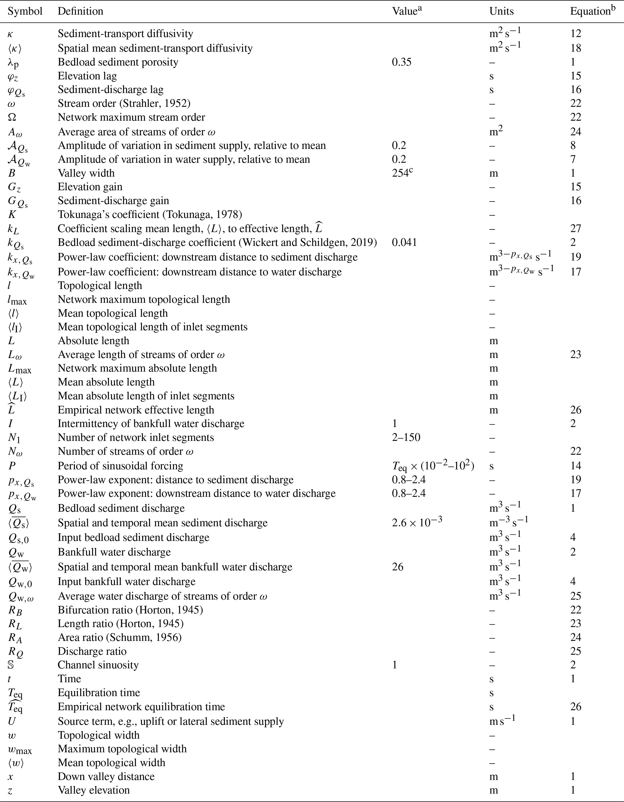
^a If applicable, value or range of values used in simulations. ^b If applicable, Equation where parameter first appears or is defined. ^c For the primary simulations B was set to this value throughout the network. For the supplementary simulations with variable valley width, the mean valley width was set to this value (Figs. S10–S27).