Hillslope diffusion and channel steepness in landscape evolution models

The streampower (SP) fluvial erosion model is the basis for many landscape evolution simulations and analyses. It assumes that river incision into bedrock depends only on flow intensity and rock erodibility and is insensitive to sediment flux. In two dimensions, the SP model is often coupled with diffusion processes, which together describe the evolution of channels and hillslopes. In a widely used formulation, the SP model and hillslope diffusion are applied everywhere while tracking only topography (the SPD model). In this case channels may steepen to erode deposited hillslope material. We conduct the first systematic investigation of this effect and use a scaling analysis to demonstrate that the increase in channel steepness can be predicted from model parameters when diffusion is linear. Alternative approaches to channel–hillslope coupling include fully detachment-limited models where channels have unlimited capacity to transport hillslope sediment, as well as models where transport capacity is limited but erosion processes differ for sediment and bedrock. A model of the latter type shows that both distinguishing bedrock and sediment erodibility and allowing for some sediment retention in channels weaken or eliminate the increase in channel steepness due to hillslope diffusion. This highlights that the SPD scaling emerges from an unlikely set of circumstances in which sediment is as hard to erode as bedrock but cannot redeposit or affect conditions downslope. A test at field sites where an SPD model adequately describes the spacing of first-order valleys shows that channels steepen to transport hillslope sediment, but the SPD scaling does not hold. This suggests that the separate treatment of sediment and bedrock and the consideration of factors such as grain size that affect sediment erodibility may be essential for predicting channel steepness using coupled channel–hillslope models.

1 Introduction

Detachment-limited erosion models are widely used to simulate and interpret how climate and tectonics affect bedrock river-long profiles. Such models assume that rivers evolve only to erode bedrock and that sediment does not affect the rate of incision (Sklar and Dietrich, 1998). Detachment-limited erosion models may be formulated in terms of excess shear stress (Whipple and Tucker, 1999; Howard and Kerby, 1983) or streampower (Seidl and Dietrich, 1992; Howard, 1994). Such assumptions reduce to a common model form, in which fluvial erosion is proportional to the product of discharge (often replaced with drainage area) to a power and slope to a power. Here we refer to this type of model as the streampower (SP) model.

In two dimensions, topography is mostly composed of hillslopes, which form due to erosion processes not driven by concentrated water flow. These hillslope processes are most often represented in landscape evolution models (LEMs) with conservation laws in which the sediment flux varies linearly or nonlinearly with slope, making them diffusional processes. For simplicity and computational efficiency, many LEMs that couple SP erosion and hillslope diffusion track only the topographic surface (Tucker et al., 2001; Perron et al., 2008; Campforts et al., 2017; Bovy and Lange, 2023). However, this leads to a conceptual challenge, as the SP model alone assumes everything eroded is bedrock, while the diffusion model alone assumes everything eroded and deposited is sediment.

One coupling approach for such models is to prevent or remove material deposited in channels by diffusion, equivalently assuming that channels have unlimited capacity to transport hillslope sediment (Campforts et al., 2017). A similar approach is to treat channels as boundary conditions for hillslopes (Perron, 2011; Goren et al., 2014; Ferrier and Perron, 2020). Such approaches produce channels and hillslopes that behave according to their independent governing equations, linked by the baselevel that channels provide to hillslopes. This can be advantageous for use or comparison with analytical solutions (Royden and Perron, 2013; Goren et al., 2014) but does not allow hillslopes to influence channel dynamics.

The more common coupling approach for models tracking only topography is to apply hillslope diffusion to every grid cell, including those that contain channels. These combined “streampower plus diffusion” (SPD) models are governed by nonlinear advection–diffusion equations, which allow for dynamic two-way coupling between channels and hillslopes but have the limitation that channels must erode deposited hillslope sediment as if it were bedrock. SPD models have been used for a wide range of geomorphologic problems. These include explaining the controls on drainage reorganization (Lyons et al., 2020) and the evolution of orogens (Wolf et al., 2022), projecting site-specific erosion (Barnhart et al., 2020b), and calibrating LEMs to topography and erosion rates globally (Ruetenik et al., 2023). Diffusion is sometimes included to aid in stability or reduce slope and elevation near drainage divides, where the SP model alone predicts that channel elevation goes to infinity as the area goes to zero (Salles, 2016; Fernandes et al., 2019). Others have added complexity to the hydrological processes used to generate discharge but have maintained the SPD erosion form to simulate the evolution of small watersheds (Litwin et al., 2022, 2024) and entire continental orogens (Shen et al., 2021). With such diverse use cases, the SPD model has become something of a “null model” for channel–hillslope landscape evolution (Barnhart et al., 2020a, 2019; Bovy and Lange, 2023).

The two-way coupling of channels and hillslopes in SPD models is widely acknowledged to be involved with setting the drainage density and valley spacing (Perron et al., 2008, 2009; Theodoratos et al., 2018; Theodoratos and Kirchner, 2020; Bonetti et al., 2020). The effect of this coupling on channel profiles has received less attention, though it has long been established that the effect can be substantial. Howard (1994, their Fig. 5A) showed one parameter combination for which the SPD model increased slope throughout the channel network compared to the SP model and identified that slope increased in order to remove deposited hillslope material. Persistent increases in slope, integrated over a basin, lead to substantial increases in total relief, and thus the chosen model coupling approach can have substantial effects on the resulting topography. Despite early demonstration of this SPD model feature, it has not been systematically described, nor is there currently a way to predict SPD channel slope from model parameters. A systematic description of how diffusion affects channel profiles could improve the interpretation of SPD model results in the growing number of applications where they can be found.

Distinguishing sediment from bedrock adds model complexity but eliminates some of the conceptual challenges of coupling that result from only tracking topography. In such models, deposited hillslope material is explicitly treated as sediment, and the fluvial model can be used to determine how sediment should be transported and how bedrock should be eroded. This also allows for the simulation of mixed bedrock–alluvial rivers that are widely observed in the field (e.g., Miller, 1991; Wohl, 1992; Snyder et al., 2000). Mixed bedrock–alluvial rivers exhibit combinations of detachment-limited behavior and transport-limited behavior (e.g., Willgoose et al., 1991) in which sediment supply exceeds transport capacity. Models have been developed that allow for transitions between transport- and detachment-limited behaviors, tracking sediment flux (e.g., Beaumont et al., 1992; Braun and Sambridge, 1997; Tucker et al., 2001; Whipple and Tucker, 2002); sediment flux and sediment bed cover (e.g., Howard, 1994; Egholm et al., 2013); or sediment flux, bed cover, and water column concentration (Davy and Lague, 2009; Shobe et al., 2017). Sometimes complex models can be reduced to simpler forms for large-scale applications. For example, Yuan et al. (2019) developed a solution to the erosion–deposition model of Davy and Lague (2009) that treats flux implicitly in order to use efficient algorithms for streampower-based erosion (Braun and Willett, 2013).

The goal of this paper is to investigate how hillslope diffusion affects channel profiles in two-dimensional LEMs. We focus primarily on the SPD model, and determine whether these effects meaningfully change how model results should be interpreted. Rather than quantifying differences in channel slope, we use channel steepness, the coefficient that relates slope and concavity-normalized drainage area. Generalizing the finding of Howard (1994), we show that hillslope diffusion can strongly affect steady-state channel steepness across a wide range of parameter combinations. We then build on an earlier scaling analysis (Litwin et al., 2022) to demonstrate that this effect can be predicted directly from model parameters when diffusion is linear (the “SPLD” – streampower plus linear diffusion – model). We contrast the SPD model predictions with a model of hillslopes and mixed bedrock–alluvial rivers using SPACE (Stream Power with Alluvium Conservation and Entrainment) (Shobe et al., 2017), which explicitly distinguishes sediment and bedrock and can retain sediment in the channel network. We show these features reduce the sensitivity of channels to local hillslope processes. Lastly, we examine several field sites where the SPLD model can correctly predict the spacing of first-order valleys (Perron et al., 2009) in order to assess the applicability of the channel–hillslope coupling in the SPD model. Our results suggest that hillslope sediment does affect channel steepness in such settings but that factors not captured by the SPD model limit the applicability of the predicted scaling between the diffusivity and channel steepness.

2 Theory and methods

2.1 Streampower model and channel steepness

The basic SP model for the evolution of channel elevation z with along-channel distance x is

$$\begin{array}{}\text{(1)}& {\displaystyle \frac{\partial z}{\partial t}}=-K{A}^m{S}^n+U,\end{array}$$

where t is time, K is the streampower incision coefficient, A(x) is the upslope area, S(x) is the channel slope, U is the uplift or baselevel change, and m and n are the area and slope exponents. At steady state, the SP model predicts a power law relationship between slope and area:

$$\begin{array}{}\text{(2)}& {\displaystyle }S=k_{sn}{A}^{-m/n},\text{(3)}& {\displaystyle }{k}_{sn,\mathrm{pred}}={\left(U/K\right)}^{\mathrm{1}/n},\end{array}$$

where k_sn is the normalized steepness index, and k_sn,pred is the predicted steepness based on the SP model. Independent of model form, k_sn can be estimated directly from regression of log-transformed slope and area using Eq. (2). Alternatively, it can be estimated from regression of elevation and the area-normalized distance coordinate χ, which minimizes noise that arises from the elevation derivative (Perron and Royden, 2013):

$$\begin{array}{}\text{(4)}& {\displaystyle }z\left(x\right)=z\left(x_{\mathrm{b}}\right)+{\left({\displaystyle \frac{U}{K{A}_{\mathrm{0}}^m}}\right)}^{\mathrm{1}/n}\mathit{\chi },\text{(5)}& {\displaystyle }\mathit{\chi }=\underset{x_{\mathrm{b}}}{\overset{x}{\int }}{\left({\displaystyle \frac{A_{\mathrm{0}}}{A\left(x\right)}}\right)}^{m/n}\mathrm{d}x,\end{array}$$

where x_b is an arbitrary baselevel location, and A₀ is a reference drainage area. The slope of the relationship between χ and z reduces to k_sn,pred when A₀=1. In order for χ to have units of L, A₀ should have units of L², in which case k_sn,pred would be dimensionless. However here we always report k_sn according to Eq. (3), which has SI units of m${}^{\mathrm{2}m/n}$. The numerical value will be the same as if A₀=1 m².

2.2 Streampower plus linear diffusion (SPLD) model

The SPLD model generalizes the SP model to two dimensions and adds a linear diffusion term to describe hillslope sediment transport:

$$\begin{array}{}\text{(6)}& {\displaystyle \frac{\partial z}{\partial t}}=-K{A}^m|\mathrm{\nabla }z{|}^n+D{\mathrm{\nabla }}^{\mathrm{2}}z+U,\end{array}$$

where D is the hillslope diffusivity and ∇ is the gradient operator. In two dimensions, we can also write a constraint that describes the relationship between elevation and the specific area a (e.g., Bonetti et al., 2020, their Eq. 5):

$$\begin{array}{}\text{(7)}& {\displaystyle }-\mathrm{\nabla }\cdot \left(a{\displaystyle \frac{\mathrm{\nabla }z}{\left|\mathrm{\nabla }z\right|}}\right)=\mathrm{1}.\end{array}$$

The specific area is the intrinsic counterpart of drainage area, defined as the drainage area per unit contour width in the limit that the contour width is small. Because it is an intrinsic property of the topographic surface, replacing area in Eq. (6) with the specific area produces a governing equation that is independent of grid resolution (Bonetti et al., 2020). Bonetti et al. (2018) describe a way to estimate a by integration of the contour curvature, but for numerical landscape evolution simulations in which a is recalculated many times, it is more efficient to estimate $a\approx A/v_{\mathrm{0}}$ from an algorithmic solution for drainage area A and grid cell width v₀. For this reason it will be helpful to write Eq. (6) explicitly accounting for the grid cell width, as in Litwin et al. (2022):

$$\begin{array}{}\text{(8)}& {\displaystyle \frac{\partial z}{\partial t}}=-K{v}_{\mathrm{0}}^m{a}^m|\mathrm{\nabla }z{|}^n+D{\mathrm{\nabla }}^{\mathrm{2}}z+U.\end{array}$$

2.3 Model setup

The goal of our main simulations is to understand the systematic differences between steady-state channels in the SPLD model (Eq. 8) and those predicted by the SP model. We will run the SPLD model with a range of parameters, extract the large channels from steady-state topography, and use χ analysis to determine their steepness, which we can compare to the predicted SP steepness (Eq. 3). We ran simulations on raster grids using the open-source Earth surface modeling platform Landlab (Hobley et al., 2017; Barnhart et al., 2020a). Fluvial erosion is calculated using an implicit scheme with D8 flow routing based on Braun and Willett (2013). Linear diffusion is calculated using an explicit finite volume scheme and applied to all cells except the external boundaries. The two processes (plus the source term U) are loosely coupled to calculate total topographic change in each time step. As previously described, hillslope diffusion is applied everywhere, allowing for net erosion when the Laplacian is negative (hilltops) and net deposition when it is positive (valleys). While the SPD models have been solved simultaneously (e.g., Perron et al., 2008), loosely coupled schemes are far more common (Tucker et al., 2001; Barnhart et al., 2019; Bovy and Lange, 2023).

All SPLD model results use a domain size of 200×400 cells, while the actual domain length varies with the grid cell width. The top and bottom edges are fixed-elevation boundaries, and the left and right are zero-flux boundaries. All model runs use the same initial condition: a randomly seeded rough surface with a mean elevation of 20 cm. We run simulations for 250 t_g (the characteristic SPLD timescale; see Sect. 3.2), at which point all simulations show negligible change in relief with time. We used Landlab to calculate the χ coordinate for locations with drainage areas greater than 100 cells. This threshold was chosen to ensure the analysis was conducted on relatively large channels with linear relationships between χ and elevation. More complex schemes could be devised to estimate the threshold for what is a channel (Passalacqua et al., 2010; Clubb et al., 2014), but we found little variation in our results for different threshold values once the threshold was sufficiently large. We estimated the normalized steepness index from χ and elevation using linear regression.

3 Results

3.1 Hillslope diffusion increases channel steepness

Stream channels extracted from steady-state results of the SPLD model have higher normalized steepness k_sn and relief than predicted by the SP model, consistent with the difference in slope observed by Howard (1994). Figure 1a shows one simulation with this behavior. Here $K=\mathrm{5}\times {\mathrm{10}}^{-\mathrm{5}}$ yr⁻¹, D=0.011 m² yr⁻¹, U=0.0005 m² yr⁻¹, m=0.5, n=1, and v₀=20 m. This corresponds to an active landscape with efficient erosion process rates. Typical K values used in SPLD models are 10⁻⁸–10⁻⁵ m^(1−2m) yr⁻¹ (Ruetenik et al., 2023), and D values of $\mathrm{4.4}\times {\mathrm{10}}^{-\mathrm{4}}$–$\mathrm{3.6}\times {\mathrm{10}}^{-\mathrm{2}}$ m² yr⁻¹ have been reported (Fernandes and Dietrich, 1997). The ratio $m/n$ is commonly 0.4–0.6, generally with n≥1 (Harel et al., 2016). In streampower-based modeling studies, m=0.5 and n=1 are commonly used as a baseline configuration (e.g., default in Landlab; Hobley et al., 2017; Barnhart et al., 2020a). As we will show later, individual parameter values in the SPLD model are less important for behavior than combinations that make up the model characteristic scales (Theodoratos et al., 2018; Litwin et al., 2022).

Differences between SP and SPLD channels in Fig. 1 are visualized in three ways. In the inset plot of Fig. 1a, an extracted channel profile is compared with the profile that would be expected from the one-dimensional SP model with the same K, U, m, n, and upslope area. In this particular channel, SPLD relief is nearly twice that of the equivalent SP model despite the fact that topography looks advection-dominated. The increase in k_sn is also apparent from the intercept of log-scaled slope and area (Fig. 1b) and slope of the χ–elevation relationship (Fig. 1c). Both show near doubling of k_sn in comparison to the SP model prediction.

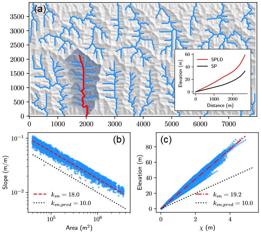
Figure 1 Visualizing the increase in channel steepness associated with hillslope processes for the model simulation with $K=\mathrm{5}\times {\mathrm{10}}^{-\mathrm{5}}$ yr⁻¹, D=0.011 m² yr⁻¹, U=0.0005 m² yr⁻¹, m=0.5, n=1, and v₀=20 m. (a) Hillshade of steady-state topography, where channels with drainage area >100 cells are highlighted in blue. Inset plot shows the profile of the channel highlighted in red compared with that expected without hillslope processes (black). The basin has approximately twice the relief of that without hillslope processes. (b) Increase in slope at a given area for all channels, compared to the prediction from the SP model (k_sn,pred). (c) Increase in channel elevation relative to expectations from the χ coordinate in comparison to the prediction from the SP model. The units of k_sn are m${}^{\mathrm{2}m/n}$.

Beyond this single case, we found that the SPLD channel steepness varies systematically with model parameters. Figure 2 shows variation in diffusivity and grid cell width for different values of the predicted SP channel steepness k_sn,pred and different combinations of m and n. The streampower incision coefficient K varies with both k_sn,pred and n. Increasing diffusivity alone increases the SPLD channel steepness in nearly all cases, but the sensitivity depends on other parameters. When k_sn,pred is small (when K is large), SPLD channel steepness is closer to the predicted SP value. The sensitivity of k_sn to diffusivity is greatest when the fluvial incision is weakly sensitive to slope (n=0.6), even despite the fact that the corresponding K values are larger than in the other streampower exponent cases.

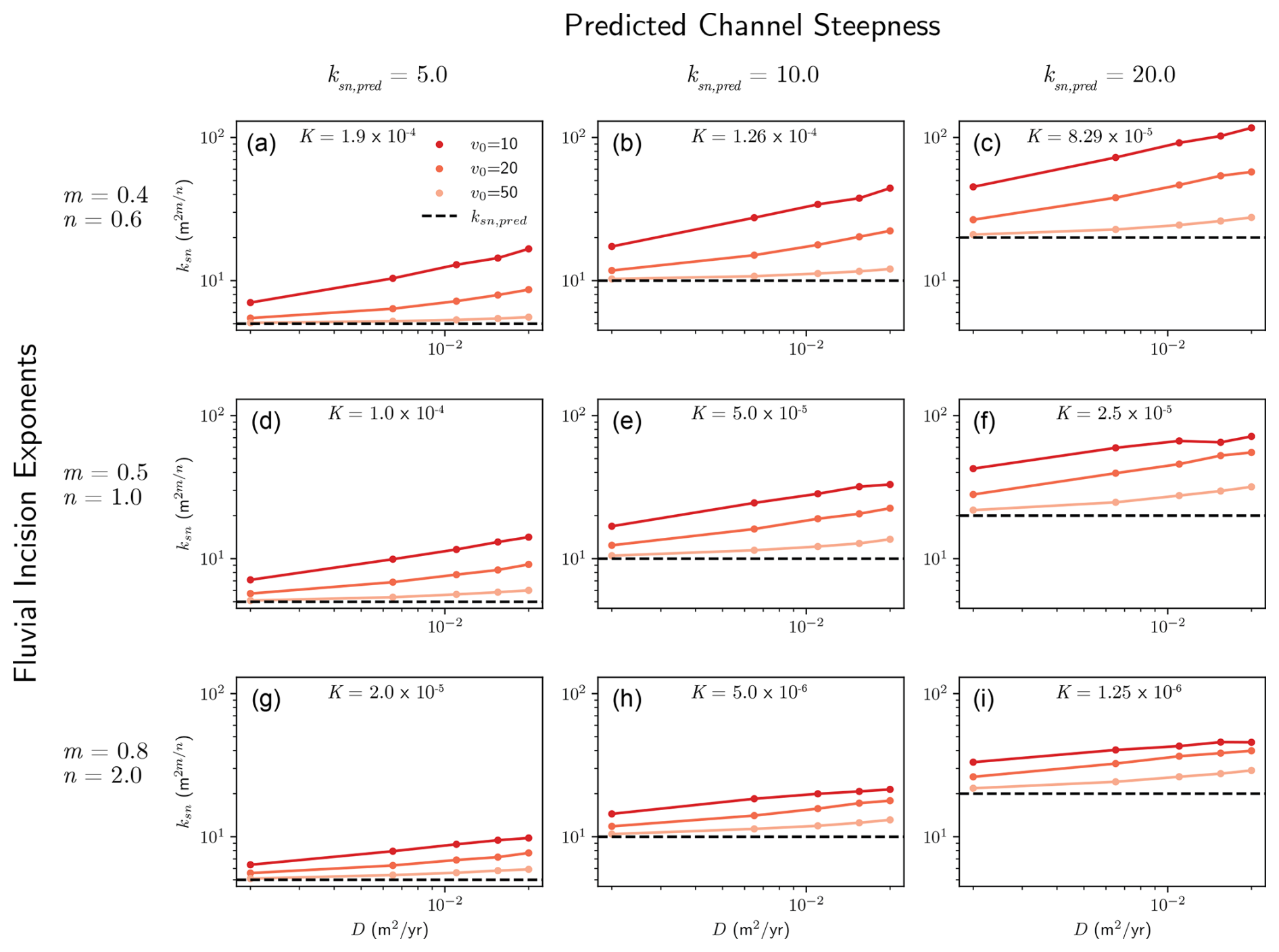
Figure 2 Increase in steady-state normalized channel steepness from the SPLD model with hillslope diffusivity D and grid cell width v₀ (colors) for three values of the predicted SP channel steepness k_sn,pred (columns) and three combinations of the streampower exponents m and n (rows). Panels have different values of K according to the combination of n and k_sn,pred (Eq. 3). The uplift rate U is held constant. The units of v₀ are meters, and the units of K are m^1−2m yr⁻¹.

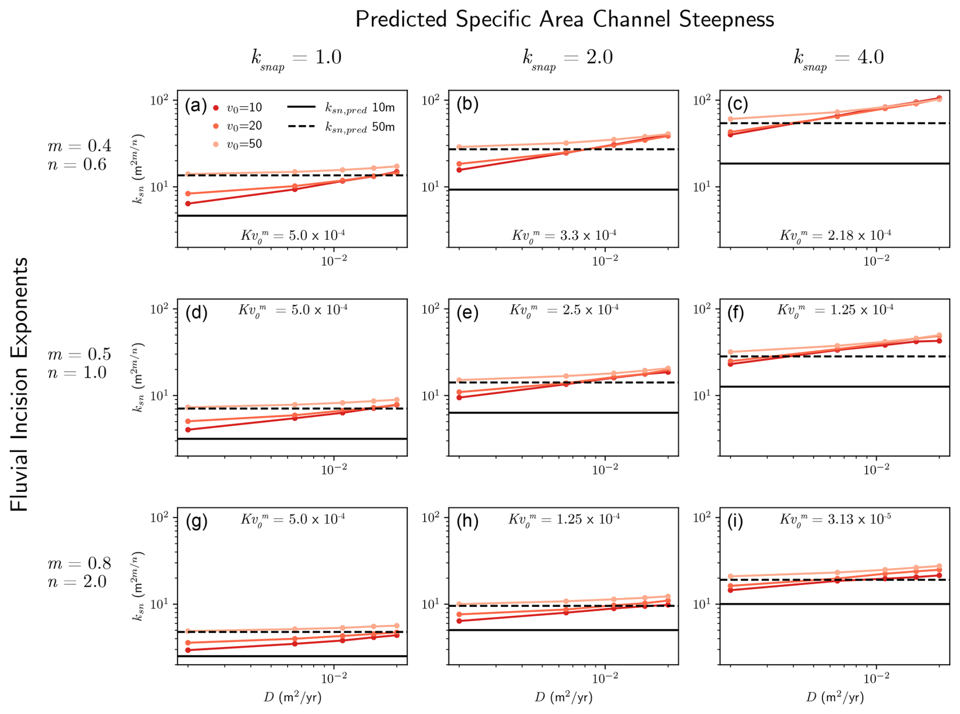
Figure 3 Variation in channel steepness k_sn with D and v₀ for several values of the specific area steepness k_snap, as defined in Eq. (11), and three different combinations of m and n. Curves with different values of v₀ have different k_sn,pred in order to conserve the quantity $K{v}_{\mathrm{0}}^m$ within each panel. We show the largest k_sn,pred (for v₀=50 m) and the smallest (for v₀=10 m) for reference.

SPLD channel steepness also increases with the grid cell width v₀. When the grid cell width is large, the channel steepness can remain close to the SP model prediction, though this diminishes as K becomes small or D becomes large. Several works have already addressed the grid cell dependence of the SPLD model (Howard, 1994; Perron et al., 2008; Pelletier, 2010; Hergarten, 2020; Hergarten and Pietrek, 2023). As others have already noted (e.g., Hergarten and Pietrek, 2023), the combination of fluvial erosion and hillslope diffusion is the source of the grid cell dependency of the SPLD model.

We can compensate for the grid cell dependence of the SPLD model by holding the quantity $K{v}_{\mathrm{0}}^m$ constant when varying v₀ (Bonetti et al., 2020). Holding this term constant implies that at different grid cell widths, we need different values of the SP steepness $k_{sn,\mathrm{pred}}=(U/K{)}^{\mathrm{1}/n}$ in order to achieve the same SPLD steepness, expressed in the relationship between slope and area or χ and elevation. We define a new steepness quantity, the specific area steepness k_snap, that will remain constant even while k_sn,pred varies, beginning with the one-dimensional streampower model at steady state:

$$\begin{array}{}\text{(9)}& {\displaystyle }\mathrm{0}=& {\displaystyle }-K{v}_{\mathrm{0}}^m{a}^m{S}^n+U,\text{(10)}& {\displaystyle }S=& {\displaystyle }{\left({\displaystyle \frac{U}{K{v}_{\mathrm{0}}^m}}\right)}^{\mathrm{1}/n}{a}^{-m/n},\end{array}$$

where again a is the specific area. Then the specific area steepness is the coefficient on slope:

$$\begin{array}{}\text{(11)}& k_{\mathrm{snap}}={\left({\displaystyle \frac{U}{K{v}_{\mathrm{0}}^m}}\right)}^{\mathrm{1}/n}.\end{array}$$

Figure 3 shows that keeping $K{v}_{\mathrm{0}}^m$ constant does reduce the dependence of steepness on the grid spacing but does not eliminate it in all cases. Even when the relative change in steepness with grid size is small (Fig. 3c), the results are still sensitive to diffusivity D, suggesting this is a characteristic feature of the SPLD model. More work could be done to further explore the scaling analysis with the specific area version of the model, but as we will show in the discussion, there are reasons to be generally skeptical of the physical realism of the scaling that emerges from the SPLD model with or without grid dependence correction.

3.2 Prediction and scaling of SPLD channel steepness

The steady-state channel steepness for the SP model can be derived directly from rearranging the SP model (Eq. 3); however, no equivalent solution exists for the SPLD model. In theory, the SPLD steepness can be derived by rearranging Eq. (6) for the relationship between slope and drainage area:

$$\begin{array}{}\text{(12)}& S={\left({\displaystyle \frac{U+D{\mathrm{\nabla }}^{\mathrm{2}}z}{K}}\right)}^{\mathrm{1}/n}{A}^{-m/n}.\end{array}$$

This shows that in channels where Laplacian curvature is positive there is net deposition of material eroded from hillslopes, so the steepness must be greater than in the SP model alone (Eq. 3). This is what we have seen in Figs. 1 and 2. We can quantify this difference by plotting the diffusion term relative to uplift. Figure 4a shows this for part of the watershed highlighted in Fig. 1, revealing that the deposition in valley bottoms locally increases the uplift rate “experienced” by the channels by a factor of 2 because the deposited sediment is not distinguished from bedrock.

We can generalize the insight expressed in Fig. 4 for pointwise calculations of the diffusion relative to uplift in order to explain the difference between SPLD and SP model steepness. We do this by taking an average of the diffusion term over channelized cells, which is possible because the hillslope flux divergence is generally poorly correlated with drainage area once drainage area is large (Fig. 4b), even while the relationship between the diffusion term and streampower term remains linear to balance uplift (Theodoratos et al., 2018). We denote the mean for locations with drainage area > 100 cells with (∼), such that $\left(D\stackrel{\mathrm{̃}}{{\mathrm{\nabla }}^{\mathrm{2}}z}\right)/U$ is the mean diffusion relative to uplift in these locations.

To quantify the difference between SP and SPLD channels, we define the steepness deviation $(k_{sn}/k_{sn,\mathrm{pred}}{)}^n-\mathrm{1}$. Note that this reduces to the relative error formula ($k_{sn}-k_{sn,\mathrm{pred}})/k_{sn,\mathrm{pred}}$ when n=1. The equivalence of $\left(D\stackrel{\mathrm{̃}}{{\mathrm{\nabla }}^{\mathrm{2}}z}\right)/U$ and the steepness deviation can be confirmed using the SPLD steepness shown in Eq. (12), focusing only on the channels:

$$\begin{array}{}\text{(13)}& k_{sn}={\left({\displaystyle \frac{U+D\stackrel{\mathrm{̃}}{{\mathrm{\nabla }}^{\mathrm{2}}z}}{K}}\right)}^{\mathrm{1}/n}.\end{array}$$

Substituting k_sn and k_sn,pred (Eq. 3) into the steepness deviation, we find

$$\begin{array}{}\text{(14)}& \begin{array}{rl}{\displaystyle }{\left({\displaystyle \frac{k_{sn}}{k_{sn,\mathrm{pred}}}}\right)}^n-\mathrm{1}& {\displaystyle }={\left[{\displaystyle \frac{{\left(\frac{U+D\stackrel{\mathrm{̃}}{{\mathrm{\nabla }}^{\mathrm{2}}z}}{K}\right)}^{\mathrm{1}/n}}{{\left(\frac{U}{K}\right)}^{\mathrm{1}/n}}}\right]}^n-\mathrm{1}\\ {\displaystyle }& {\displaystyle }={\displaystyle \frac{U+D\stackrel{\mathrm{̃}}{{\mathrm{\nabla }}^{\mathrm{2}}z}}{U}}-\mathrm{1}={\displaystyle \frac{D\stackrel{\mathrm{̃}}{{\mathrm{\nabla }}^{\mathrm{2}}z}}{U}}.\end{array}\end{array}$$

Figure 5a, d, and g show that the mean hillslope diffusion term relative to uplift in channels predicts the steepness deviation well for model runs in Fig. 2. Each panel in Fig. 5 aggregates all values of K, D, and v₀ shown in rows of Fig. 2. Most points fall very close to the 1:1 line, while some points with large average diffusion in channels have a lower than expected steepness deviation. These cases have relatively low dissection, and it is assumed that model boundary conditions are beginning to affect the relief and channel steepness.

While these results confirm a simple rearrangement of the governing equation, the channel curvature $\stackrel{\mathrm{̃}}{{\mathrm{\nabla }}^{\mathrm{2}}z}$ is generally not known prior to simulation. More useful would be to estimate the steepness deviation from the model parameters alone, which we can do using scaling analyses of the SPLD model equations. Litwin et al. (2022) presented a dimensional analysis of Eqs. (7) and (8) with m=0.5 and n=1 that uses characteristic scales for horizontal length ℓ_g, height h_g, and time t_g. Here we generalize this for any values of the exponents m and n. This dimensional analysis follows Theodoratos et al. (2018) in identifying three separate dimensions of the model: time T applies to t; height H applies to z; and horizontal length L applies to a, v₀, and the horizontal coordinates x and y. The coefficients in Eq. (8) can be rewritten in terms of characteristic height, length, and timescales h_g, ℓ_g, and t_g such that each term on the right has the same units as the time derivative of elevation $H/T$.

$$\begin{array}{}\text{(15)}& {\displaystyle \frac{\partial z}{\partial t}}={\displaystyle }-{\displaystyle \frac{h_{\mathrm{g}}^{\mathrm{1}-n}{\mathrm{\ell }}_{\mathrm{g}}^{n-m}}{t_{\mathrm{g}}}}{a}^m|\mathrm{\nabla }z{|}^n+{\displaystyle \frac{{\mathrm{\ell }}_{\mathrm{g}}^{\mathrm{2}}}{t_{\mathrm{g}}}}{\mathrm{\nabla }}^{\mathrm{2}}z+{\displaystyle \frac{h_{\mathrm{g}}}{t_{\mathrm{g}}}},\end{array}$$

where we also assign the gradient operator units of $\mathrm{1}/L$. A system of equations can be defined by setting the coefficients of the terms on the right-hand side of Eq. (15) equal to those in Eq. (8).

$$\begin{array}{}\text{(16)}& \begin{array}{rl}{\displaystyle }U=& {\displaystyle \frac{h_{\mathrm{g}}}{t_{\mathrm{g}}}}\\ {\displaystyle }D=& {\displaystyle \frac{{\mathrm{\ell }}_{\mathrm{g}}^{\mathrm{2}}}{t_{\mathrm{g}}}}\\ {\displaystyle }K{v}_{\mathrm{0}}^m=& {\displaystyle \frac{h_{\mathrm{g}}^{\mathrm{1}-n}{\mathrm{\ell }}_{\mathrm{g}}^{n-m}}{t_{\mathrm{g}}}}\end{array}\end{array}$$

Solving this system, the characteristic scales are the following for positive exponents m and n:

$$\begin{array}{}\text{(17)}& {\displaystyle }{\mathrm{\ell }}_{\mathrm{g}}=& {\displaystyle }{\left({\displaystyle \frac{D^n{U}^{\mathrm{1}-n}}{K{v}_{\mathrm{0}}^m}}\right)}^{\mathrm{1}/(m+n)},\text{(18)}& {\displaystyle }{h}_{\mathrm{g}}=& {\displaystyle }{\left({\displaystyle \frac{D^{n-m}{U}^{\mathrm{2}+m-n}}{K^{\mathrm{2}}{v}_{\mathrm{0}}^{\mathrm{2}m}}}\right)}^{\mathrm{1}/(m+n)},\text{(19)}& {\displaystyle }{t}_{\mathrm{g}}=& {\displaystyle }{\left({\displaystyle \frac{D^{n-m}{U}^{\mathrm{2}-\mathrm{2}n}}{K^{\mathrm{2}}{v}_{\mathrm{0}}^{\mathrm{2}m}}}\right)}^{\mathrm{1}/(m+n)}.\end{array}$$

When $m=\mathrm{1}/\mathrm{2}$ and n=1, the characteristic scales reduce to those identified by Litwin et al. (2022).

Critical to our analysis is the characteristic horizontal length scale ℓ_g, which quantifies the distance from the ridge at which there is a transition in relative importance from diffusive to advective processes. ℓ_g is analogous to the SPLD horizontal length scale derived by Perron et al. (2009) and Theodoratos et al. (2018), which we call ℓ_c. Only ℓ_g comes from the version using specific area a (Eqs. 7, 8), and ℓ_c comes from the version using area A (Eq. 6):

$$\begin{array}{}\text{(20)}& {\displaystyle }{\mathrm{\ell }}_{\mathrm{c}}={\displaystyle }{\left({\displaystyle \frac{D^n{U}^{\mathrm{1}-n}}{K}}\right)}^{\mathrm{1}/(\mathrm{2}m+n)}.\end{array}$$

The relationships in Fig. 2 show that the channels are steeper in comparison to the SP model prediction when diffusive processes are stronger relative to advective processes and that steepness is also inversely proportional to the grid cell width. These results also hold for those where $K{v}_{\mathrm{0}}^m$ is held constant (Fig. 3) because the underlying solution is the same. Using the characteristic scales, we found ℓ_c (Eq. 20) normalized by v₀ is not only proportional to the steepness deviation $(k_{sn}/k_{sn,\mathrm{pred}}{)}^n-\mathrm{1}$ but is approximately equal to it (Fig. 5b, e, h). In the SPLD model ℓ_c is an important control on the spacing of first-order valleys (Perron et al., 2009); it appears to be an important control on channel steepness in the model as well.

The length scale ℓ_g (Eq. 17) derived for the SPLD model with specific area performs slightly better than ℓ_c overall (Fig. 5c, f, i). The root mean squared error (RMSE) and log-transformed RMSE (RMSLE) suggest ${\mathrm{\ell }}_{\mathrm{c}}/v_{\mathrm{0}}$ and ${\mathrm{\ell }}_{\mathrm{g}}/v_{\mathrm{0}}$ are comparable predictors, but visual inspection suggests the trend in steepness deviation with ${\mathrm{\ell }}_{\mathrm{g}}/v_{\mathrm{0}}$ is more aligned with the 1:1 line than the trend with ${\mathrm{\ell }}_{\mathrm{c}}/v_{\mathrm{0}}$. This is likely related to the dependence of ℓ_g on v₀. The ratio ${\mathrm{\ell }}_{\mathrm{c}}/v_{\mathrm{0}}$ implies scaling of the steepness deviation with $v_{\mathrm{0}}^{-\mathrm{1}}$, while using ${\mathrm{\ell }}_{\mathrm{g}}/v_{\mathrm{0}}$ implies scaling with $v_{\mathrm{0}}^{-(\mathrm{2}m+n)/(m+n)}$.

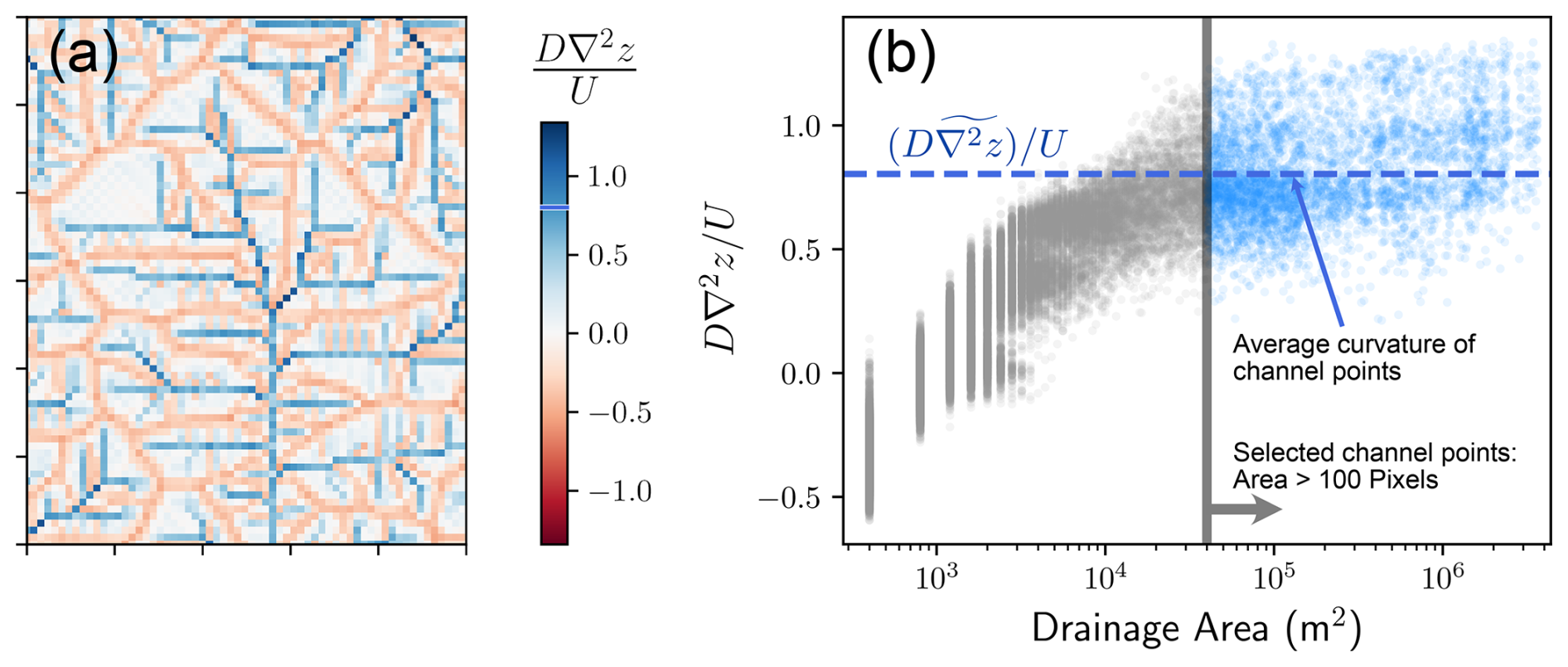
Figure 4 (a) The diffusion term relative to uplift for part of the highlighted watershed shown in Fig. 1. In valley bottoms, the diffusion term is net depositional and is nearly equal to the uplift rate. (b) The diffusion term relative to uplift versus drainage area, showing that they are not strongly correlated for large drainage areas. Points colored blue have drainage area > 100 cells, and a mean value is shown with a dashed blue line. The mean line also appears on the colorbar of (a).

The equivalence of the steepness deviation and ${\mathrm{\ell }}_{\mathrm{g}}/v_{\mathrm{0}}$ then implies that ${\mathrm{\ell }}_{\mathrm{g}}/v_{\mathrm{0}}$ is approximately equal to the channel-averaged diffusion term relative to uplift $D\stackrel{\mathrm{̃}}{{\mathrm{\nabla }}^{\mathrm{2}}z}/U$. Consequently the SPLD channel-averaged curvature can also be estimated from model parameters. Making one further substitution suggests another interesting relationship between model parameters and curvature. At hilltops, where drainage area goes to zero, the steady-state curvature is ${\mathrm{\nabla }}^{\mathrm{2}}{z}_h=-U/D$. Substituting the hilltop curvature −∇²z_h for $U/D$, we find

$$\begin{array}{}\text{(21)}& {\displaystyle \frac{{\mathrm{\ell }}_{\mathrm{g}}}{v_{\mathrm{0}}}}{\displaystyle }\approx {\displaystyle \frac{D\stackrel{\mathrm{̃}}{{\mathrm{\nabla }}^{\mathrm{2}}z}}{U}}=-{\displaystyle \frac{\stackrel{\mathrm{̃}}{{\mathrm{\nabla }}^{\mathrm{2}}z}}{{\mathrm{\nabla }}^{\mathrm{2}}{z}_h}}.\end{array}$$

Thus the model predicts that ${\mathrm{\ell }}_{\mathrm{g}}/v_{\mathrm{0}}$ is approximately the ratio of channel-to-hilltop curvatures.

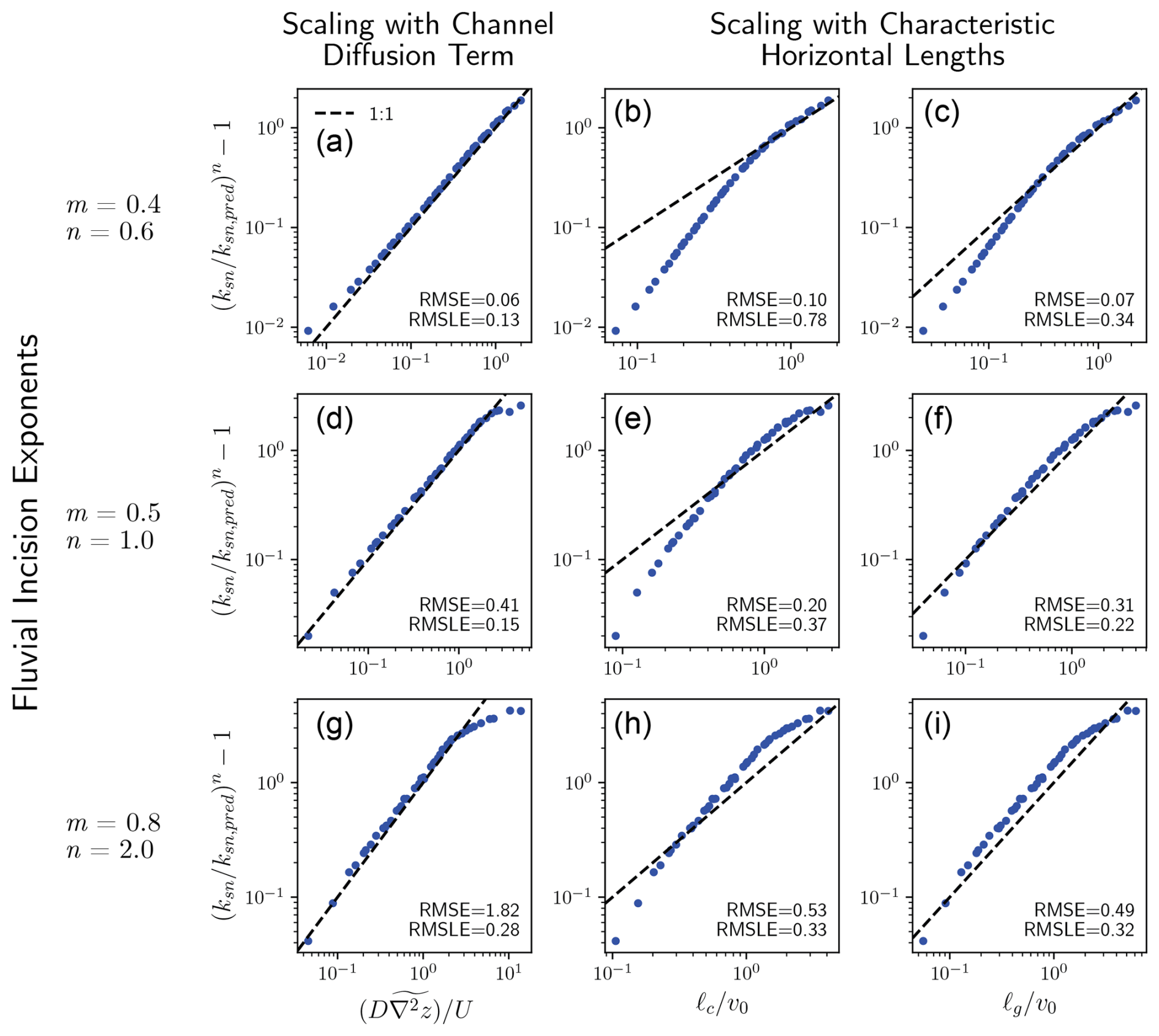
Figure 5 (a, d, g) The average of the diffusion term in channels relative to uplift (see Fig. 4) versus the steepness deviation. Each panel in a row contains points from all columns in the corresponding row of Fig. 2. (b, e, h) The length scale ℓ_c (Eq. 20) relative to the grid cell width explains the steepness deviation. (c, f, i) The length scale ℓ_g (Eq. 17) relative to the grid cell width explains the steepness deviation. RMSE is the root mean squared error, and RMSLE is the log-transformed RMSE.

The scaling results suggest there is an inherent trade-off in the SPLD model. Studies have chosen ${\mathrm{\ell }}_{\mathrm{c}}/v_{\mathrm{0}}$ or ${\mathrm{\ell }}_{\mathrm{g}}/v_{\mathrm{0}}$ to be greater than 1 in order to resolve the diffusive-to-advective transition that occurs downstream of ridges (Theodoratos et al., 2018; Litwin et al., 2022). When the ratio is equal to 1 and n=1, SPLD steepness is already double the SP steepness. This may reflect actual channel–hillslope coupling (we will discuss this further in the next sections), but it may also lead to unexpected behavior. For instance, if K and D are both increased for a simulation where lithology is perceived to be softer and more weatherable, the steady-state relief may increase or decrease depending on their ratio and the value of n, following the scaling in Fig. 5.

In contrast, if one chooses parameter values such that ${\mathrm{\ell }}_{\mathrm{c}}/v_{\mathrm{0}}$ or ${\mathrm{\ell }}_{\mathrm{g}}/v_{\mathrm{0}}$ is small, hillslopes will not be fully resolved, and numerical diffusion, rather than the explicit hillslope diffusion, becomes important. For some large-scale applications, this may be fine, as it satisfies the need to prevent elevation from going to infinity as drainage area goes to zero. In any case, understanding how the channel–hillslope coupling will affect the simulated results should be an important part of SPLD model use, especially for understanding how the results contrast with intuitions developed from the SP model.

Finally, while we have focused on coupling the SP model with linear diffusion, the scaling has explanatory power for nonlinear diffusion as well. The most common nonlinear hillslope diffusion is the critical slope model (Andrews and Bucknam, 1987; Roering et al., 1999):

$$\begin{array}{}\text{(22)}& {\displaystyle \frac{\partial z}{\partial t}}=D\mathrm{\nabla }\cdot {\displaystyle \frac{\mathrm{\nabla }z}{\mathrm{1}-\left(\right|\mathrm{\nabla }z|/S_{\mathrm{c}}{)}^{\mathrm{2}}}},\end{array}$$

where S_c is the critical slope. A more numerically tractable Taylor expansion of this model was proposed by Ganti et al. (2012):

$$\begin{array}{}\text{(23)}& {\displaystyle \frac{\partial z}{\partial t}}=D\mathrm{\nabla }\cdot \left[\mathrm{\nabla }z\left(\mathrm{1}+{\left({\displaystyle \frac{\left|\mathrm{\nabla }z\right|}{S_{\mathrm{c}}}}\right)}^{\mathrm{2}}\right)\right],\end{array}$$

which they showed to be a close approximation of the original partial differential equation for small S. When we run simulations with the same parameter values shown in Figs. 2 and 5 but replace the linear diffusion term with the Taylor expansion model (Eq. 23) with S_c=0.5, we find that simulated channels tend to fall at or above the 1:1 line (Fig. 6); i.e., nonlinear diffusion with a critical slope increases channel steepness relative to the SP solution at least as much as suggested by the SPLD scaling.

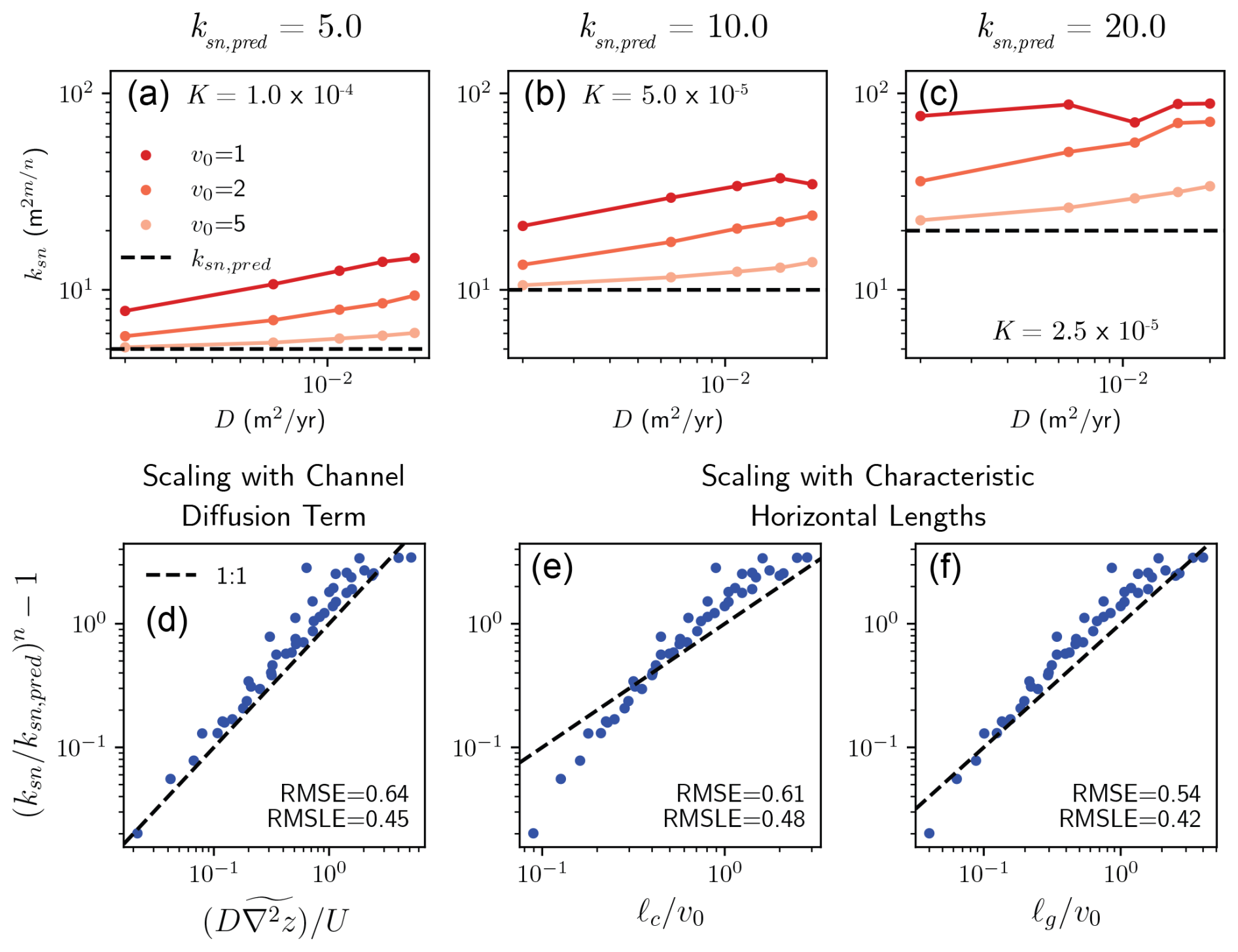
Figure 6 (a, b, c) Increase in steady-state normalized channel steepness from the SPLD model with hillslope diffusivity D and grid cell width v₀ (colors) for three values of the predicted SP steepness k_sn,pred. Diffusion is a nonlinear, second-order Taylor expansion of the critical slope model (Ganti et al., 2012), and the critical slope is 0.5. All results shown have m=0.5 and n=1.0. The units of v₀ are meters, and the units of K are m^1−2m yr⁻¹. Compare with Fig. 2d, e, and f, which have the same parameters but use linear diffusion. (d, e, f) Scaling relationships at steady state. (d) The diffusion term relative to uplift averaged over channels (∼) versus the steepness deviation. Most sites have a steepness deviation greater than or equal to that suggested by the linear diffusion analytical solution. (e) The deviation explained with the characteristic length scales ℓ_c from Theodoratos et al. (2018) and (f) ℓ_g from Litwin et al. (2022). Compare with Fig. 5d, e, and f.

4 Discussion

4.1 Physical interpretation of SPLD channel–hillslope coupling

As we have established, the widely used version of the SPLD model studied here couples channels and hillslopes by applying fluvial and hillslope processes in every cell. This has been justified with the sub-grid concept that each cell contains one segment of channel and adjacent hillslopes, though models do not explicitly resolve such sub-grid features (Howard, 1994). Conceptually, the cell elevation is then the average of the channel and hillslope component elevations. Hergarten (2020) states that the hillslope flux may be effectively only distributed on the hillslope components of the cell (Perron et al., 2008; Howard, 1994) or only on the channel component (Pelletier, 2010) in order to reduce scale dependence of the model. Assuming that channels must ultimately transport hillslope material to maintain mean cell elevation at steady state, the two sub-grid representations still have the effect that sediment must be removed before erosion can begin to counter rock uplift.

In this sense, the SPLD model channel–hillslope coupling is a kind of sediment cover effect. However, because the SPLD model couples mass-conserving hillslope diffusion with non-mass-conserving fluvial erosion, this cover effect is strictly local; i.e., while using a spatially and temporally uniform K implies sediment is as difficult to erode as bedrock, the eroded material cannot deposit and does not continue to affect conditions downstream. Past studies have argued that this is appropriate for applications where the domain of interest is small enough that redeposition can be ignored and where sediment has similar erodibility to bedrock (Perron et al., 2008). However, the SPLD model has been used in scaling analyses and applications at much larger scales (Theodoratos et al., 2018; Theodoratos and Kirchner, 2020; Wolf et al., 2022; Shen et al., 2021). The question of applicability at small scales is also in doubt. In reality, there is sediment retained at every scale in the fluvial system, and such sediment retention can affect channel properties even in headwaters (Sklar, 2024). Furthermore, cases where the travel distances of sediment particles are long are also likely to have finer grain sizes and consequently a higher erodibility of sediment relative to bedrock, making the combination of features of the SPD model unlikely.

In the following section, we discuss how hillslope diffusion affects channels using alternate coupling strategies, focusing on cases where hillslope diffusion is still applied everywhere, but sediment and bedrock erosion are tracked separately. Finally, we examine what field data can tell us about the appropriate channel–hillslope coupling approach using sites where the SPLD model scaling adequately predicts the spacing of first-order valleys.

4.2 Distinguishing eroded materials and conserving sediment mass

As previously described, several alternate approaches are available to couple channels with hillslopes in LEMs. One solution would be to prevent deposition by diffusion in channels (Campforts et al., 2017). This still allows diffusion to limit steady-state elevation as the area goes to zero and results in streams that conform to the SP model's analytical solutions. This is also useful for simulation of channels and hillslopes where the channels should maintain channel steepness and relief estimated by analysis of channel-long profiles (e.g., Harel et al., 2016). However, this approach eliminates most of the capacity of diffusive processes to balance advective fluvial processes. Because channels are assumed to have unlimited capacity to transport hillslope sediment, the critical area for channel formation must be chosen as a parameter rather than emerging as a result of competition between advection and diffusion.

An alternate approach is to represent, in some fashion, the erosion and deposition of sediment independently from bedrock (e.g., Beaumont et al., 1992; Tucker et al., 2001; Shobe et al., 2017; Yuan et al., 2019). Ideally, the simulation should be able to smoothly transition between bedrock and alluvial behavior based on the availability of sediment. Here we use one such model, Stream Power with Alluvium Conservation and Entrainment (SPACE; Shobe et al., 2017), coupled with hillslope diffusion, and contrast the sensitivity of channel steepness to hillslope processes under different configurations. SPACE maintains a relatively simple formulation but explicitly tracks sediment mass balance and captures the reduction in bedrock incision due to sediment cover. It has steady-state analytical solutions for channel steepness in mixed bedrock–alluvial conditions (Appendix A) to which we can compare the numerical results of SPACE coupled with linear diffusion (“SPACE plus diffusion”).

We considered three different variables from SPACE: K_s is the streampower coefficient for sediment, K_r is the coefficient for bedrock, and V is the average net-downward velocity of sediment grains. Setting V=0 creates a detachment-limited condition identical to the SP model alone, as entrained sediment cannot redeposit. Setting V=5 m yr⁻¹ represents coarse sediment that may redeposit. An additional parameter to characterize sediment, F_f, describes the fraction of sediment derived from bedrock erosion that is permanently suspended and not considered in the mass balance. As such, detachment-limited conditions can also be achieved by setting F_f=1.0, though we will not show these results here.

We use a square 100×100 domain with three zero-flux boundaries and one fixed-value boundary on the lower edge to maximize the size of drainage basins within the domain. Simulations are run with a 30 m grid cell width and 25 yr time steps for 2 Myr. We set m=0.5, n=1.0, U=0.0005 m yr⁻¹, D=0.05 m² yr⁻¹, $K_{\mathrm{r}}=\mathrm{1}\times {\mathrm{10}}^{-\mathrm{4}}$ yr⁻¹, and F_f=0. All additional SPACE parameters were held constant and are given in Appendix A. We assumed all material deposited by hillslope diffusion had the same properties as sediment produced by bedrock erosion. This is the same approach that Shobe et al. (2017) used in a two-dimensional demonstration.

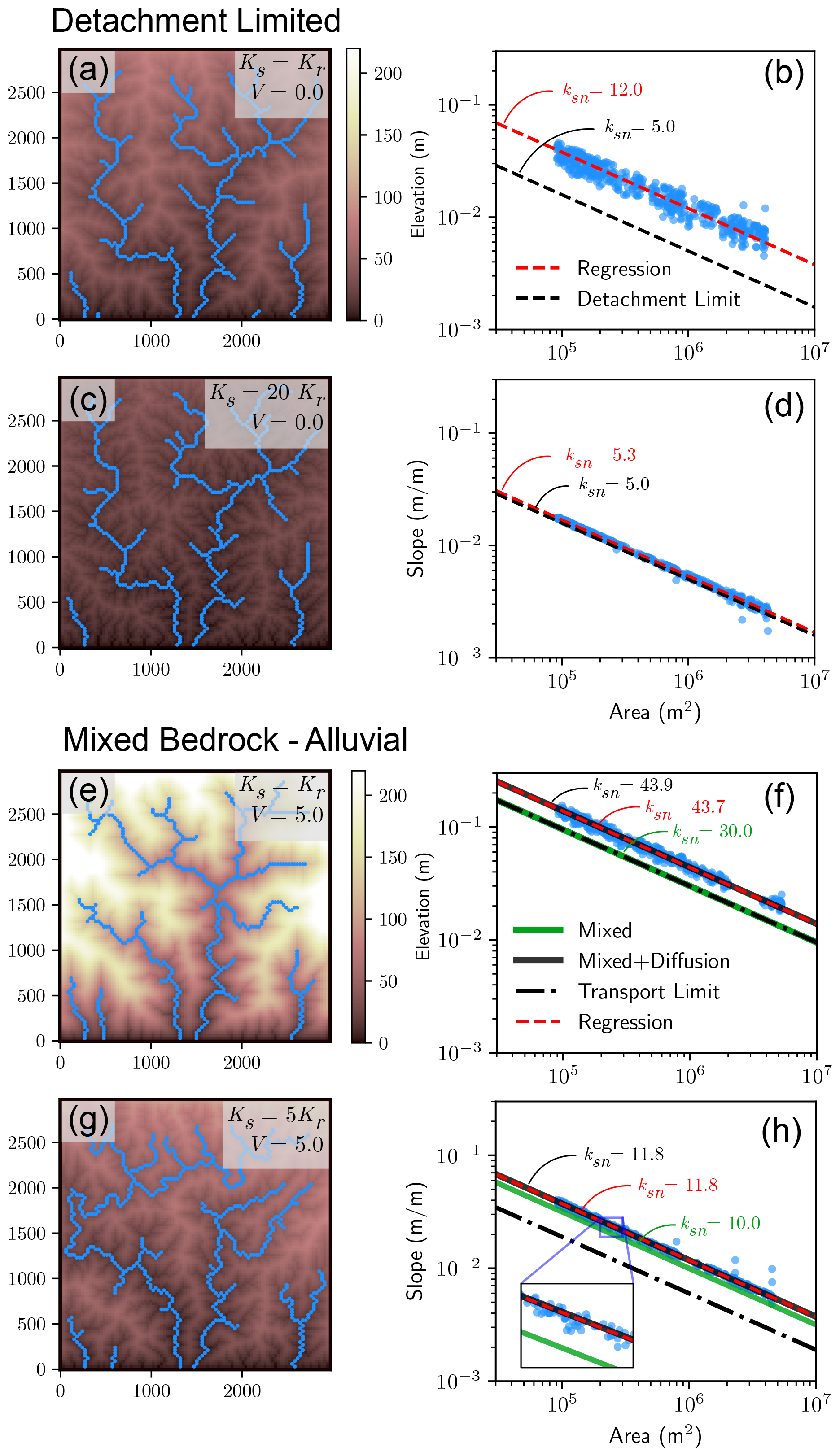
Figure 7 SPACE–diffusion model results, showing elevation with locations where drainage area is > 100 cells highlighted in blue (left column) and slope–area relationships (right column). (a, b) The case most similar to the SPD model, with no redeposition of fluvially entrained sediment (V=0). (c, d) Same as (a, b) but sediment is much more erodible than bedrock. (e, f) Sediment has the same erodibility as bedrock and may redeposit in the model domain (V=5.0 m yr⁻¹). (g, h) Same as (e, f) but sediment is more erodible than bedrock. The “detachment limit” solution (Eq. A1) is the same as the SP model. The “transport limit” (Eq. A2) and “mixed” (Eq. A3) solutions come from SPACE alone, while “mixed plus diffusion” solution (Eq. A9) includes diffusion through a semi-analytical solution that relies on modeled channel curvature.

Figure 7 shows topography and channel slope–area relationships for four simulations using SPACE plus diffusion. The first case (Fig. 7a, b) is analogous to the SPLD model: sediment and bedrock erodibility are the same (K_s=K_r), and sediment cannot be redeposited once it is suspended (V=0). The equilibrium channel steepness estimated from regression is 12.0 m, more than twice the detachment-limited prediction (Eq. A1) of 5.0 m, which is the same as k_sn,pred when K is replaced with K_r in Eq. (3). The modeled steepness is significantly higher because sediment deposited by hillslope processes must still be entrained (K_s=K_r) before it can be transported away without redeposition (V=0). The second case (Fig. 7c, d) is the same as the first, except we increased the erodibility of sediment (K_s=20K_r). This erodibility contrast is more reasonable for fine sediment that does not redeposit after entrainment. As a result, the steepness increase from hillslope sediment is minimal. Here, the channel steepness is 5.3 m, very close to the predicted value of 5.0 m.

Next we set V>0.0 as an example of mixed bedrock–alluvial rivers in which entrained fluvial sediment may redeposit, affecting bed cover and consequently steady-state channel slope. The first case with V=5.0 m yr⁻¹ (Fig. 7e, f) is otherwise the same as Fig. 7a and b. Because sediment and bedrock erodibility are equal, the analytical solutions for mixed bedrock–alluvial equilibrium steepness (Eq. A3) and transport-limited equilibrium steepness (Eq. A2) are equivalent: k_sn=30.0 m. This is significantly higher than the detachment-limited cases (Fig. 7b, d) but also relatively closer to the coupled SPACE–diffusion steepness of 43.7 m. This discrepancy can be explained too, as shown with the semi-analytical “mixed plus diffusion” line, which we will explain more below.

When the sediment is 5 times more erodible than bedrock (Fig. 7g, h), it is clearer that the SPACE–diffusion channel steepness approaches the mixed bedrock–alluvial analytical solution (Eq. A3). Here the analytical solution predicts a channel steepness of 10.0 m, and the channel steepness from regression is 11.8 m. In other words, when sediment mass is conserved, the effect of the particular diffusivity or length of adjacent hillslopes on channel slope diminishes compared to the need to transport sediment from upstream. Similarly, when Guryan et al. (2024) compared the steepness of SP and SPACE model channels eroding through layered stratigraphy, they found that accounting for sediment diminished the difference in steepness between hard and soft lithologies.

Why is there still an offset between equilibrium steepness of mixed bedrock–alluvial channels and the analytical solution (“mixed” line, Fig. 7f, h) if all upslope sediment is already accounted for regardless of hillslope diffusion? The residual deviation is due to the bed cover effect in SPACE. While diffusivity does not affect the total amount of sediment that must leave the watershed at a given drainage area, it does add an additional flux term to the local sediment mass balance. The SPACE model alone predicts that the steady-state sediment thickness is spatially uniform (Appendix A, Eq. A4). The addition of diffusion causes steady-state sediment thickness to increase relative to the SPACE solution in valleys where the hillslope flux is net positive and decrease on ridges where the hillslope flux is net negative. Indeed, the average channel sediment thicknesses for simulations in Fig. 7e and g are 2.2 and 1.0 m respectively; the SPACE analytical solutions for steady-state thickness without diffusion are 1.8 and 0.8 m respectively.

Based on the assumption that diffusion affects sediment cover but minimally affects total downstream sediment transport, we re-derive the steepness for mixed bedrock–alluvial channels coupled with linear diffusion (Appendix A, Eq. A9). The results are shown with the solid black “mixed plus diffusion” lines in Fig. 5f and h. This is not a fully analytical solution, as it relies on the same principle of averaging channel curvature that we used to produce the results in Fig. 5a, d, and g. However, it supports our conceptualization of the model behavior, as the predicted steepness is nearly identical to that calculated from the regression.

While the mechanism by which channel steepness is affected by sediment is different in the SPACE plus diffusion and SPD models, the result may be hard to distinguish in steady-state profiles, as is the case more generally with detachment and transport-limited models (Whipple and Tucker, 2002). The benefit of a model such as SPACE is that the strength of the interaction between channel steepness and hillslope sediment can be explained and its relative importance explored through model parameters with clearer links to lithology in terms of sediment characteristics (the effective settling velocity V and the fraction of fine sediment F_f) or climate in terms of weathering and sediment production. This may be especially important in transient simulations where there is a greater distinction between detachment and transport-limited behavior.

In real landscapes, the effect of local sediment input from hillslopes seems to be especially important in settings with large sediment inputs from landslides. Ott et al. (2024) show that incision thresholds associated with the delivery of landslide-derived sediment to channels decrease the sensitivity of channel steepness to erosion rate in the northern Andes. The effect of discrete two-dimensional landslides on channel-long profiles is explored by Campforts et al. (2020), who also use SPACE. In another modeling study, Shobe et al. (2018) found that the sensitivity of channel steepness to erosion rate is also reduced by uplift-rate-dependent incision thresholds caused by the delivery of hillslope-derived boulders to rivers.

These studies and the effects we have discussed here with SPACE and the SP model focus on the importance of sediment cover in limiting erosion. However, sediment grains moving with flowing water are the necessary tools for bedrock erosion (Sklar and Dietrich, 2004; Lamb et al., 2015). This effect is implicitly included in SPACE and SP models in that sediment discharge may scale with water discharge and drainage area. However, fully addressing the effect of sediment on coupled channel–hillslope evolution including the tools' effect is an important direction for future landscape evolution modeling (Gasparini et al., 2004; Egholm et al., 2013; Roy et al., 2016). Furthermore, bedrock rivers exhibit co-adjustment of width, steepness, and sediment cover, which also mediates the effectiveness of sediment tools (e.g., Lavé and Avouac, 2001; Johnson and Whipple, 2010; Yanites et al., 2010). Dynamic bedrock channel width adjustment has been implemented for channel profiles (Yanites, 2018) but remains challenging in two-dimensional channel–hillslope models.

4.3 Relevance to channel–hillslope coupling in the field

Field evidence that rivers steepen in order to transport hillslope sediment generally comes from settings where lithologies of contrasting strength move through river networks (Johnson et al., 2009; Finnegan et al., 2017; Lai et al., 2021). That supports a channel–hillslope coupling strategy where hillslope sediment can deposit in channels, but it is not a scenario that SPD models can represent. Can we still observe river steepening due to hillslope sediment in more lithologically homogeneous settings that are suited to the SPD model? We have also shown that the SPD channel–hillslope coupling results in a scaling between fluvial erodibility, diffusivity, and uplift in ℓ_c or ℓ_g. Our demonstration with the SPACE plus diffusion model suggests that this relationship is easily weakened or eliminated by differences in sediment and bedrock erodibility or by the redeposition of eroded fluvial sediment. Does the SPD channel steepness scaling hold in settings best suited to the model? Here we attempt to answer these questions at several sites where we think the SPD model is most likely to explain channel–hillslope dynamics based on the fact that the length scale ℓ_c derived from topography correlates well with the spacing of first-order valleys (Perron et al., 2009), as predicted by the model.

In order to answer these questions, we need independent ways to assess actual channel steepness and the expected steepness in the absence of hillslope processes $k_{sn,\mathrm{pred}}=(U/K{)}^{\mathrm{1}/n}$. Otherwise the value of K in ℓ_c would already reflect potential influences of hillslope sediment. However, most studies only estimate $(U/K{)}^{\mathrm{1}/n}$ from channel steepness (e.g., Harel et al., 2016). One exception is the method derived by Perron et al. (2009) to estimate $D/K$ from topography when n=1 by introducing the solution for diffusivity from hilltop curvature $U/D\approx {\mathrm{\nabla }}^{\mathrm{2}}{z}_h$ into the SPLD model (Eq. 6):

$$\begin{array}{}\text{(24)}& {\displaystyle \frac{\left|\mathrm{\nabla }z\right|}{{\mathrm{\nabla }}^{\mathrm{2}}z-{\mathrm{\nabla }}^{\mathrm{2}}{z}_h}}={\displaystyle \frac{D}{K}}{A}^{-m},\end{array}$$

from which they estimated m and $D/K$ by least squares regression. These terms are then used to estimate ℓ_c (their L_c). Because the model used to derive Eq. (24) assumes n=1, we can estimate the predicted channel steepness k_sn,pred:

$$\begin{array}{}\text{(25)}& k_{sn,\mathrm{pred}}={\displaystyle \frac{U}{K}}={\displaystyle \frac{D}{K}}{\displaystyle \frac{U}{D}}\approx {\displaystyle \frac{D}{K}}{\mathrm{\nabla }}^{\mathrm{2}}{z}_h.\end{array}$$

The approximation in the hilltop curvature relationship is due to the conversion of rock to regolith, which have different bulk densities. Typical ratios of rock-to-regolith bulk density are 1.5–2 (Roering et al., 2007; Heimsath et al., 1997). However, if the bulk density of the material eroded by fluvial processes is equal to that of bedrock, as assumed in the SP model, then U and K have the same bulk density prefactors and the conversions cancel out. Consequently the last term of Eq. (25) is exactly equal to k_sn,pred (see Appendix B). Assuming uniform K, D, and U, we can compare k_sn,pred in Eq. (25) to the steepness of larger channels adjacent to the first-order valleys that were the focus of Perron et al. (2009) to match our analysis of the SPLD model results.

We forgo direct assessment of the SPLD scaling and calculation of ℓ_g, ${\mathrm{\ell }}_{\mathrm{c}}/v_{\mathrm{0}}$, or ${\mathrm{\ell }}_{\mathrm{g}}/v_{\mathrm{0}}$ because of dependence on the grid cell width. These are model-dependent quantities whose real-world interpretation is more nebulous. For this case study we focus on general scaling expected from the SPLD model: channel steepness relative to k_sn,pred should increase with ℓ_c.

Perron et al. (2009) considered five sites with varying valley spacing. We eliminated the two sites with the smallest spacing because the first-order channels do not share baselevel with higher-order rivers. We estimated channel steepness from least squares regression of the χ–elevation relationship, where χ was calculated using the concavity index from Perron et al. (2009) so that the resulting channel steepness will be comparable with k_sn,pred in Eq. (25).

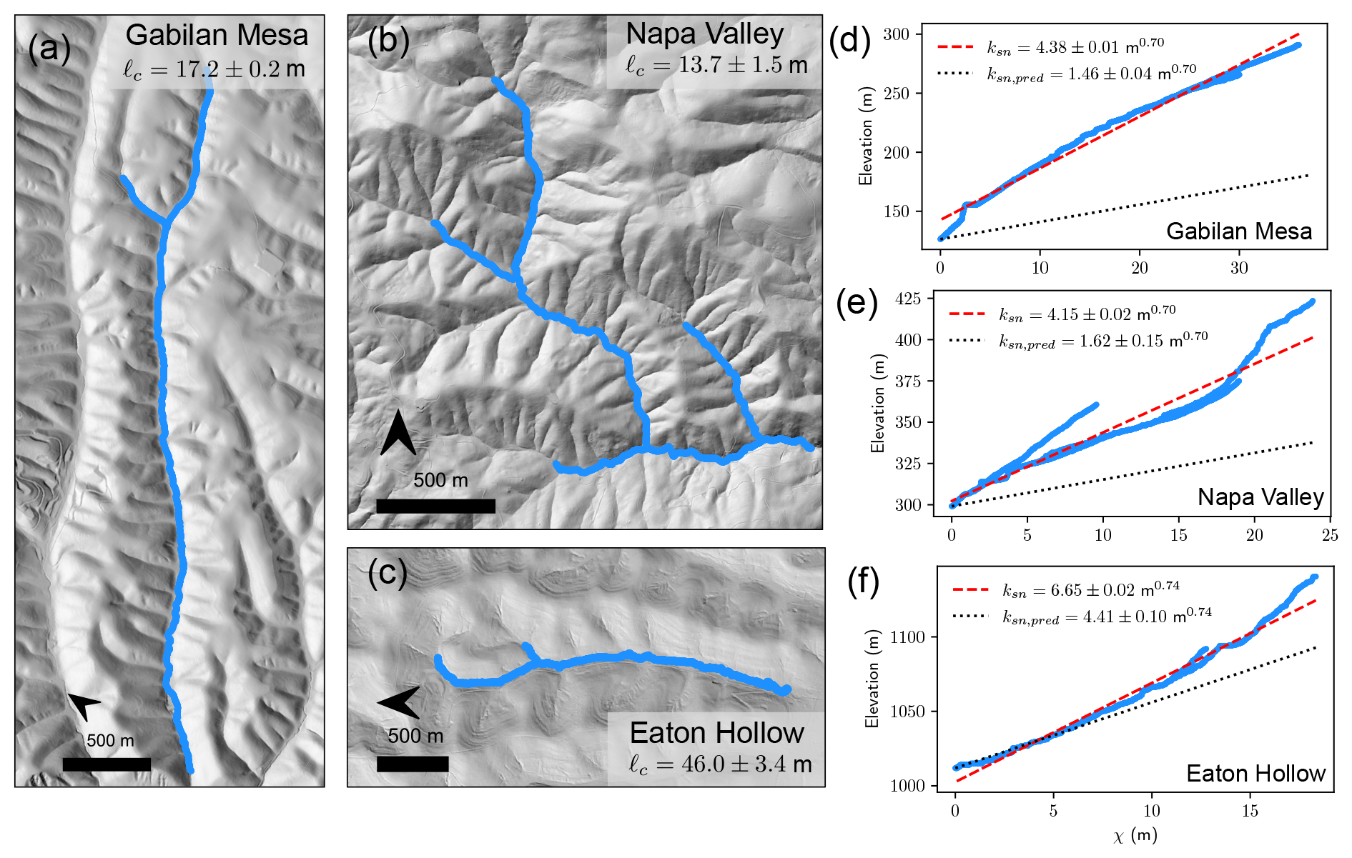
Figure 8 (a, b, c) Hillshades of Gabilan Mesa, California (35.923° N, 120.820° W); Napa Valley, California (38.508° N, 122.332° W); and Eaton Hollow, Pennsylvania (39.904° N, 80.042° W). (d, e, f) The χ–elevation profiles for blue channels highlighted in the hillshades. The concavity indices used to calculate χ are 0.35, 0.35, and 0.37 respectively (Perron et al., 2009). The dashed red line is a linear regression, where slope gives an estimate of channel steepness. The dashed black line is the predicted channel profile starting at baselevel and increasing with the steepness predicted by Eq. (25.)

All three sites have greater channel steepness than would be expected from the one-dimensional SP parameters (Fig. 8). Napa Valley has ℓ_c≈14 m and a channel steepness deviation $k_{sn}/k_{sn,\mathrm{pred}}-\mathrm{1}$ of 1.56. Gabilan Mesa is similar, with ℓ_c≈17 m and steepness deviation of 2.0. Eaton Hollow has the largest value of ℓ_c (46 m), and thus the SPLD scaling predicts the steepness deviation should be largest of the three sites. However, the steepness deviation is only 0.51.

While this is a very limited case study, it does have two important implications. First, channel steepness likely is affected by hillslope sediment, as would be predicted by many models (Sklar and Dietrich, 2006). This suggests allowing deposition of hillslope sediment in channels may be a reasonable approach for channel–hillslope LEMs. Second, even in the settings that are supposedly well-suited to the SPLD model, the model is not predictive of channel steepness.

We suggest that the limited steepness deviation at Eaton Hollow could be due to the difference in the character of the hillslope sediment. Eaton Hollow is located on the Appalachian Plateau, which has a lower denudation rate than the other two sites, and thus likely longer regolith residence times, which may lead to the production of finer, more easily transportable sediment. If this is the case, the SPACE model prediction that channel slope reduces to the detachment-limited prediction when sediment is easily erodible could be relevant. This hypothesis could be tested by extending the analysis to more sites and including grain size distribution estimates. While the SPACE–diffusion model with high sediment erodibility would predict that channel heads should be much closer to ridges at Eaton Hollow, it is possible that a threshold associated with runoff generation could be an important control on drainage density here (Litwin et al., 2022, 2024). This could be further addressed with site-based measurements of the extent of surface runoff.

5 Conclusions

Researchers using channel–hillslope LEMs must choose how fluvial and hillslope processes are coupled. This is especially critical in models that track only the topographic surface. The widely used “streampower plus diffusion” (SPD) model approaches this by applying hillslope diffusion everywhere. Hillslope diffusion is known to increase channel steepness in SPD LEMs (Howard, 1994), as channels steepen to erode deposited hillslope sediment. Here we show that this effect occurs systematically across the model parameter space and demonstrate for the first time that steady-state SPD channel steepness can be predicted from the model parameters when diffusion is linear (the SPLD model). SPLD channel steepness relative to SP steepness increases with the characteristic length scale of the SPLD model (Perron et al., 2009; Theodoratos et al., 2018; Litwin et al., 2022) relative to the grid cell width. This prediction still holds for the formulation of the SPLD model that reduces grid resolution dependence by using area per contour width rather than area as a state variable (Bonetti et al., 2020; Litwin et al., 2022), at least when area per contour width is estimated from upslope area calculated with a standard flow-routing algorithm.

While real rivers are known to steepen to accommodate sediment transport, the particular representation in SPD models is limited to cases where sediment is at once as difficult to suspend as bedrock is to detach, but once suspended, it remains so and is no longer accounted for downstream. This is a consequence of combining a mass-conserving model of hillslope processes with a non-mass-conserving model of fluvial erosion and tracking only a single topographic surface.

We relax the SPD model assumptions by considering an alternate model formulation with hillslope diffusion and mixed bedrock–alluvial rivers using SPACE (Shobe et al., 2017). We still allow hillslope diffusion to occur everywhere but distinguish sediment from bedrock for the purposes of fluvial erosion. Increasing the erodibility of sediment relative to bedrock decreases the effect of diffusion on equilibrium channel steepness by increasing the pace of sediment removal, which decreases bed cover. Allowing for sediment retention transitions rivers toward transport-limited behavior, in which equilibrium channel steepness is higher than the detachment-limited case, but diffusion has a smaller effect because channel slope adjusts to transport all upstream sediment. We find that diffusion can still increase the equilibrium sediment thickness in such cases though, which leads to smaller but still significant increases in channel steepness proportional to the net deposition of hillslope sediment in channels.

We test the applicability of the channel–hillslope coupling approach in the SPLD model by estimating the effect of hillslope sediment on channel steepness at three sites where the SPLD model correctly predicts that first-order valley spacing increases with the characteristic length scale (Perron et al., 2009). We show a modification of the method of Perron et al. (2009) to estimate what the SPLD model predicts channel steepness would be in the absence of hillslope processes. We find that the actual channel steepness is higher, suggesting that allowing hillslope sediment in channels is physically reasonable even in homogeneous lithologies. Channel steepness does not increase with the characteristic length scale though, indicating that other factors that cannot be accounted for when modeling only a single topographic surface, such as sediment grain size, are important even in these sites that appear well-suited for the SPLD model.

Despite the lack of field applicability, our steepness scaling is a powerful tool for understanding SPLD model behavior. In parts of the parameter space where the steepness scaling effect is expected to greatly affect the results or when emergent channel properties are particularly important, we recommend against drawing insights from SPD channel profiles and overall relief. For applications where one-way channel–hillslope coupling is suitable, preventing hillslope sediment deposition in channels may be an adequate solution. In other applications, improvements can be made with minimal increased complexity by distinguishing between sediment and bedrock and tracking sediment mass, as in the SPACE model. Future work on hillslope–channel coupling in two-dimensional models should consider incorporating a more explicit representation of sediment grain size, as it is a key factor linking the evolution of hillslopes and the development of channel-long profile forms.

Appendix A: SPACE steady-state solutions

The steady-state relationship between slope and area in the detachment-limited, transport-limited, and mixed bedrock–alluvial cases of the SPACE model without diffusion are given by Eqs. (40), (44), and (46) of Shobe et al. (2017) respectively. From these relationships, we can derive the steepness k_sn that relates $A^{-m/n}$ to S (Eq. 2). For the detachment-limited case, the steepness is

$$\begin{array}{}\text{(A1)}& k_{sn}={\left({\displaystyle \frac{U}{K_{\mathrm{r}}}}\right)}^{\mathrm{1}/n},\end{array}$$

where K_r is the bedrock erodibility. The transport-limited steepness is

$$\begin{array}{}\text{(A2)}& k_{sn}={\left[{\displaystyle \frac{UV}{K_{\mathrm{s}}r}}+{\displaystyle \frac{U}{K_{\mathrm{s}}}}\right]}^{\mathrm{1}/n},\end{array}$$

where V is the effective settling velocity, r is the local runoff rate, and K_s is the sediment erodibility. The mixed bedrock–alluvial solution is the same, except the second appearance of K_s is replaced with K_r:

$$\begin{array}{}\text{(A3)}& k_{sn}={\left[{\displaystyle \frac{UV}{K_{\mathrm{s}}r}}+{\displaystyle \frac{U}{K_{\mathrm{r}}}}\right]}^{\mathrm{1}/n}.\end{array}$$

The equilibrium sediment thickness for the mixed bedrock–alluvial case is (Shobe et al., 2017, Eq. 47)

$$\begin{array}{}\text{(A4)}& H=-H^{*}\log \left[\mathrm{1}-{\displaystyle \frac{V}{\frac{K_{\mathrm{s}}r}{K_{\mathrm{r}}}+V}}\right],\end{array}$$

where H^* is the bed roughness length scale. All simulations shown in Fig. 7 have r=1 m yr⁻¹, $H^{*}=\mathrm{1.0}$ m, and F_f=0.0. F_f is the fraction of fluvially eroded bedrock that was immediately suspended and removed from the mass balance. In our simulations that couple SPACE with diffusion, we found that steady-state channel steepness and sediment thickness were nearly identical whether detachment-limited erosion conditions were created by setting F_f=1.0 or setting V=0.0.

Hillslope diffusion modifies the mass balance equation for sediment thickness H. We can add diffusion to the steady-state sediment mass balance (Shobe et al., 2017, Eq. 16):

$$\begin{array}{}\text{(A5)}& {\displaystyle \frac{\partial H}{\partial t}}=\mathrm{0}=V{\displaystyle \frac{Q_{\mathrm{s}}}{Q}}-K_{\mathrm{s}}q{S}^n\left(\mathrm{1}-e^{-H/H^{*}}\right)+D{\mathrm{\nabla }}^{\mathrm{2}}z.\end{array}$$

Now we consider this balance only for large drainage areas, where we assume that the total sediment discharge at equilibrium is still equal to the total rock flux from uplift into the upslope area Q_s=UA. With this and the streampower model assumption q=k_qA^m, we find

$$\begin{array}{}\text{(A6)}& \mathrm{0}={\displaystyle \frac{VU}{r}}-K_{\mathrm{s}}{A}^m{S}^n\left(\mathrm{1}-e^{-H/H^{*}}\right)+D\stackrel{\mathrm{̃}}{{\mathrm{\nabla }}^{\mathrm{2}}z},\end{array}$$

where the coefficient k_q has been subsumed into K_s as in Shobe et al. (2017), and $\stackrel{\mathrm{̃}}{{\mathrm{\nabla }}^{\mathrm{2}}z}$ is the average channel curvature as we have defined previously. Equation (A6) can be rearranged for $\mathrm{1}-e^{-H/H^{*}}$:

$$\begin{array}{}\text{(A7)}& \mathrm{1}-e^{-H/H^{*}}={\displaystyle \frac{\frac{VU}{r}+D\stackrel{\mathrm{̃}}{{\mathrm{\nabla }}^{\mathrm{2}}z}}{K_{\mathrm{s}}{A}^m{S}^n}}.\end{array}$$

This is the same as in Shobe et al. (2017), except that $VU/r$ is replaced with $VU/r+D\stackrel{\mathrm{̃}}{{\mathrm{\nabla }}^{\mathrm{2}}z}$. Now consider the steady-state equation for bedrock elevation. We assume this is only modified by diffusion through H:

$$\begin{array}{}\text{(A8)}& {\displaystyle \frac{\partial R}{\partial t}}=\mathrm{0}=U-K_{\mathrm{r}}{A}^m{S}^n\left(\mathrm{1}-e^{-H/H^{*}}\right).\end{array}$$

Substituting Eq. (A7) into Eq. (A8) and rearranging for the coefficient that relates $A^{-m/n}$ to S, we find a modified relationship for channel steepness in mixed bedrock–alluvial channels with hillslope diffusion:

$$\begin{array}{}\text{(A9)}& k_{sn}={\left[{\displaystyle \frac{UV/r+D\stackrel{\mathrm{̃}}{{\mathrm{\nabla }}^{\mathrm{2}}z}}{K_{\mathrm{s}}}}+{\displaystyle \frac{U}{K_{\mathrm{r}}}}\right]}^{\mathrm{1}/n}.\end{array}$$

Note that this solution holds in the case where the only sediment production is from fluvial erosion of bedrock (applied everywhere in the landscape) and that hillslope sediment transport is independent of regolith thickness. In the code provided with this paper, we include the option to produce a transportable hillslope regolith with an exponential production function but do not present results of that configuration as that is out of the scope of this study. A more comprehensive treatment of hillslope sediment transport coupled with SPACE can be found in Campforts et al. (2020).

Appendix B: SPLD model with bulk density

The steady-state SPLD model can be written with bulk density conversions as

$$\begin{array}{}\text{(B1)}& \mathrm{0}=-{\mathit{\rho }}_{\mathrm{r}}K{A}^m|\mathrm{\nabla }z{|}^n+{\mathit{\rho }}_{\mathrm{s}}D{\mathrm{\nabla }}^{\mathrm{2}}z+{\mathit{\rho }}_{\mathrm{r}}U,\end{array}$$

assuming that the streampower term primarily removes bedrock with bulk density ρ_r and that hillslope sediment transport applies to regoliths with bulk density ρ_s. On hilltops the fluvial term goes to zero:

$$\begin{array}{}\text{(B2)}& \mathrm{0}={\mathit{\rho }}_{\mathrm{s}}D{\mathrm{\nabla }}^{\mathrm{2}}{z}_h+{\mathit{\rho }}_{\mathrm{r}}U,\end{array}$$

where ∇²z_h is the hilltop curvature. Eliminating U from Eq. (B1) using Eq. (B2), we find

$$\begin{array}{}\text{(B3)}& {\mathit{\rho }}_{\mathrm{r}}K{A}^m|\mathrm{\nabla }z{|}^n={\mathit{\rho }}_{\mathrm{s}}D\left({\mathrm{\nabla }}^{\mathrm{2}}z-{\mathrm{\nabla }}^{\mathrm{2}}{z}_h\right),\end{array}$$

from which we can derive the equivalent of Eq. (24) that explicitly accounts for bulk density:

$$\begin{array}{}\text{(B4)}& {\displaystyle \frac{{\mathit{\rho }}_{\mathrm{s}}}{{\mathit{\rho }}_{\mathrm{r}}}}{\displaystyle \frac{D}{K}}{A}^{-m}={\displaystyle \frac{\left|\mathrm{\nabla }z\right|}{{\mathrm{\nabla }}^{\mathrm{2}}z-{\mathrm{\nabla }}^{\mathrm{2}}{z}_h}}.\end{array}$$

Therefore the intercept of the regression between the log of area and the log of the right-hand side of Eq. (24) may actually estimate $\frac{{\mathit{\rho }}_{\mathrm{s}}D}{{\mathit{\rho }}_{\mathrm{r}}K}$. Multiplying this estimate by the hilltop curvature as we show in Eq. (25) gives $U/K$ without a bulk density prefactor:

$$\begin{array}{}\text{(B5)}& {\displaystyle \frac{{\mathit{\rho }}_{\mathrm{s}}}{{\mathit{\rho }}_{\mathrm{r}}}}{\displaystyle \frac{D}{K}}{\mathrm{\nabla }}^{\mathrm{2}}{z}_h={\displaystyle \frac{{\mathit{\rho }}_{\mathrm{s}}D}{{\mathit{\rho }}_{\mathrm{r}}K}}{\displaystyle \frac{{\mathit{\rho }}_{\mathrm{r}}U}{{\mathit{\rho }}_{\mathrm{s}}D}}={\displaystyle \frac{U}{K}}.\end{array}$$

This suggests that we can get a reasonable estimate of $U/K$ from $D/K$ and hilltop curvature from Perron et al. (2009) without further accounting for bulk density.