Sediment aggradation rates in Himalayan rivers revealed through the InSAR differential residual topographic phase

Using Interferometric Synthetic Aperture Radar (InSAR), we quantify sediment aggradation rates in the proximal gravel-rich portions of rivers draining from the Himalayan mountain front onto the Gangetic Plains. We develop a novel approach based on the differential residual topographic phase (DRTP) by implementing the small baseline subset (SBAS) InSAR method on Sentinel-1 C-band InSAR images. With this approach, we measure millimetre-scale relative elevation changes in four river channels over approximately 15 km of their length from the Himalayan mountain front downstream to the gravel–sand transition. This study is the first to apply differential residual topographic phase mapping to seasonally dry (ephemeral) rivers. These measurements record the changes that result from sediment deposition during the summer monsoon floods from 2016 to 2021. Results indicate sediment aggradation in river channels during the wet monsoon, with rates reaching up to approximately 20 mm yr⁻¹ (i.e. per monsoon) near the mountain front and decreasing to near zero downstream of the gravel–sand transition. Meanwhile, the floodplain in the basin is subsiding at varying rates that average ∼ 15 mm yr⁻¹. These findings enable a temporal understanding of sediment aggradation rates that impact river avulsion and flood risk in the plains, particularly for the rapidly growing rural communities in Nepal and Bihar, India. Our study demonstrates the feasibility of the InSAR technique for geomorphological monitoring that can act as input into flood risk modelling and management in the Gangetic Plains.

1 Introduction

In this study, we develop a novel InSAR (Interferometric Synthetic Aperture Radar) approach called differential residual topographic phase (DRTP) to study relative elevation changes due to sediment aggradation of ephemeral gravel riverbeds and their surrounding floodplains as they flow southward from the Himalayan mountain front in southeastern Nepal (Fig. 1). The DRTP approach uses the residual topographic phase of over a hundred interferograms' residual topographic phase along dry riverbeds as its signal. These data are processed through the small baseline subset (SBAS) InSAR method to record millimetre-scale changes in surface elevations as a result of sediment deposition during monsoon floods. The absolute (rather than differential) residual topographic phase has been used previously to estimate the height difference between newly deposited lava flows (≥25 m thick); this analysis used four pairs of L-band interferograms' absolute residual topographic phase and yielded an average uncertainty $\sim \pm \mathrm{9}$ m (Ebmeier et al., 2012). Absolute phase information converted into residual topography values has high uncertainty due to its linear relationship with the perpendicular baseline (Ebmeier et al., 2012). In contrast, our study uses the DRTP approach to measure elevation change by calculating the differential residual topographic phase in time-series domain with millimetre-scale accuracy. This high accuracy is based on the root mean square error of the estimated differential residual topographic phase in the time-series domain which is zero when displacement histories are linear or exponential (Fattahi and Amelung, 2013). This component of the differential residual topographic phase is generated by the variation in the perpendicular baseline.

This novel approach is built on previous key studies (Bombrun et al., 2009; Fattahi and Amelung, 2013; Du et al., 2016; Zhang et al., 2019). We leverage the different residual topographic phases as a signal rather than noise. This implies that if the residual topographic phase is preserved with high quality, the elevation change information carried within it can be obtained with zero root mean square error. This study is the first to demonstrate the extraction of elevation change information of ephemeral riverbeds from the differential residual topographic phase in the time-series domain. Accuracy is improved by using a stack of interferograms, with the difference between each year's residual topographic phase being calculated and then inverted into millimetre-scale elevation change rates.

Ephemeral rivers are dry for significant periods of time and so are characteristic of many arid and/or seasonally wet settings (Laronne and Reid, 1993). Sediment transport within ephemeral rivers is therefore limited to periods of flooding and may be associated with high sediment flux, particularly as rivers emerge from rapidly eroding mountain ranges (Allen et al., 2013). As mountain rivers discharge into surrounding plains, they deposit large accumulations of coarse sediment, forming alluvial fans or cones with a convex cross-sectional topography (Bull, 1977). The sediment that accumulates at the mountain front is associated with the transition from river channels that flow over tectonically uplifting bedrock in the range to subsiding foreland basins (Flemings and Jordan, 1989; Sinclair et al., 1991); this transition is associated with reductions in channel gradients and rapid deposition of coarse sediment loads. Sediment deposition at mountain fronts is usually characterized by coarse gravel-rich deposition until at some distance downstream there is an abrupt reduction in grain size at the gravel–sand transition (Dingle et al., 2021; Sambrook Smith and Ferguson, 1995). The position of the gravel–sand transition is interpreted to be limited by the total flux of coarse bedload discharged to the Gangetic Plains (Dingle et al., 2017).

The Himalayan mountain front is critically sensitive to sediment supplied from the mountain range as it impacts hydropower and irrigation infrastructure and modifies flood risk downstream for some of the most vulnerable communities (Dingle et al., 2020; Sinha et al., 2005). However, sediment yield from the range is poorly constrained on a decadal scale, and known changes in climate and land use including deforestation, changing agriculture, and urbanization are likely to be impacting these rates (Asselman et al., 2003; Sam and Khoi, 2022). Extreme discharge events, linked to glacial melting, landslide damming, and cloudburst events, are capable of transporting huge volumes of sediment downstream within the mountains (Graf et al., 2024; Shugar et al., 2021) and then exporting this sediment over the Gangetic Plains (Quick et al., 2023). Hence, being able to monitor changes in sediment budgets is a top priority for these regions.

The rapid accumulation of coarse sediment in the proximal parts of the Himalayan foreland basin have resulted in a long history of channel avulsion (Chakraborty et al., 2010; Sinha et al., 2005), where river channels aggrade at a faster rate than their surrounding floodplains, leading to super-elevation. Typically, super-elevation occurs when the riverbed approximates the height of the surrounding floodplain and the topographic slope perpendicular to the channel is greater than the long channel gradient (Jerolmack and Mohrig, 2007; Slingerland and Smith, 2004). Channel avulsion results in major flooding and displacement of rural communities in the Gangetic Plains. The Kosi floods of 2008 were caused by a breakout of the embanked Kosi River across its large fan system, displacing ∼ 2.5 million people (Sinha, 2009). An underlying cause of this event was sediment accumulation in the embanked channel, elevating it above the floodplains of Bihar State (Mishra and Sinha, 2020).

Understanding where channels are prone to avulsion requires knowledge of sediment aggradation rates within channels relative to surrounding floodplains. However, measurements of channel aggradation rates on 10- to 100-year timescales are challenging. Multi-temporal digital elevation models have proved valuable for quantifying geomorphic change and sediment budgets in some river systems (Wheaton et al., 2010; Williams, 2012). Similarly, repeat surveys of channel bathymetry can demonstrate longer-term changes due to erosion and sedimentation (Lane et al., 1994). Photogrammetry used to construct topography based on structure from motion can correct for water depths to enable river bathymetry to be approximated (Shintani and Fonstad, 2017). However, these approaches are not appropriate for the scale of large Himalayan rivers. Remote sensing techniques are increasingly capable of recording hydraulic and geomorphic change over large areas in river systems at high temporal resolutions (Rossi et al., 2023). A number of studies have used synthetic aperture radar (SAR) to monitor changes in channel morphology and characterize morphological characteristics such as grain size (Lin et al., 2023; Olen and Bookhagen, 2020; Purinton and Bookhagen, 2020). Here, the differential residual topographic phase (DRTP) method is applied to seasonally dry riverbeds, enabling vertical sediment aggradation rates in river channels to be compared to subsidence rates in surrounding floodplains.

2 Study area

The study area is in Madhesh Province, southeast Nepal, where we analysed four rivers draining the Siwalik Hills, labelled rivers 1–4 (Fig. 1). These rivers have relatively small catchments (20–30 km²) but are thought to have high erosion rates and sediment yields, as indicated by detrital cosmogenic nuclides data from the along-strike Siwalik Hills (Mandal et al., 2023). The rivers were selected because they are typically dry in winter months, ensuring that the riverbeds remain undisturbed and suitable for SAR measurements. The channel widths are approximately 300 m as they flow across the Gangetic Plains. The channel slope predominantly aligns north–south with a consistent slope gradient of 0.008 (vertical: horizontal), which is unlikely to cause geometric distortions in Sentinel-1 SAR images (Woodhouse, 2017). The analysis of these rivers focuses on the gravel reach and the downstream gravel–sand transition, which has been mapped in this area by Dubille and Lavé (2015). Upstream of this transition, the typical D50 grain size in the channels is around 2 cm (Dubille and Lavé, 2015; Quick et al., 2020) – a key factor in determining the backscatter signal for the InSAR methodology (see Sect. 3).

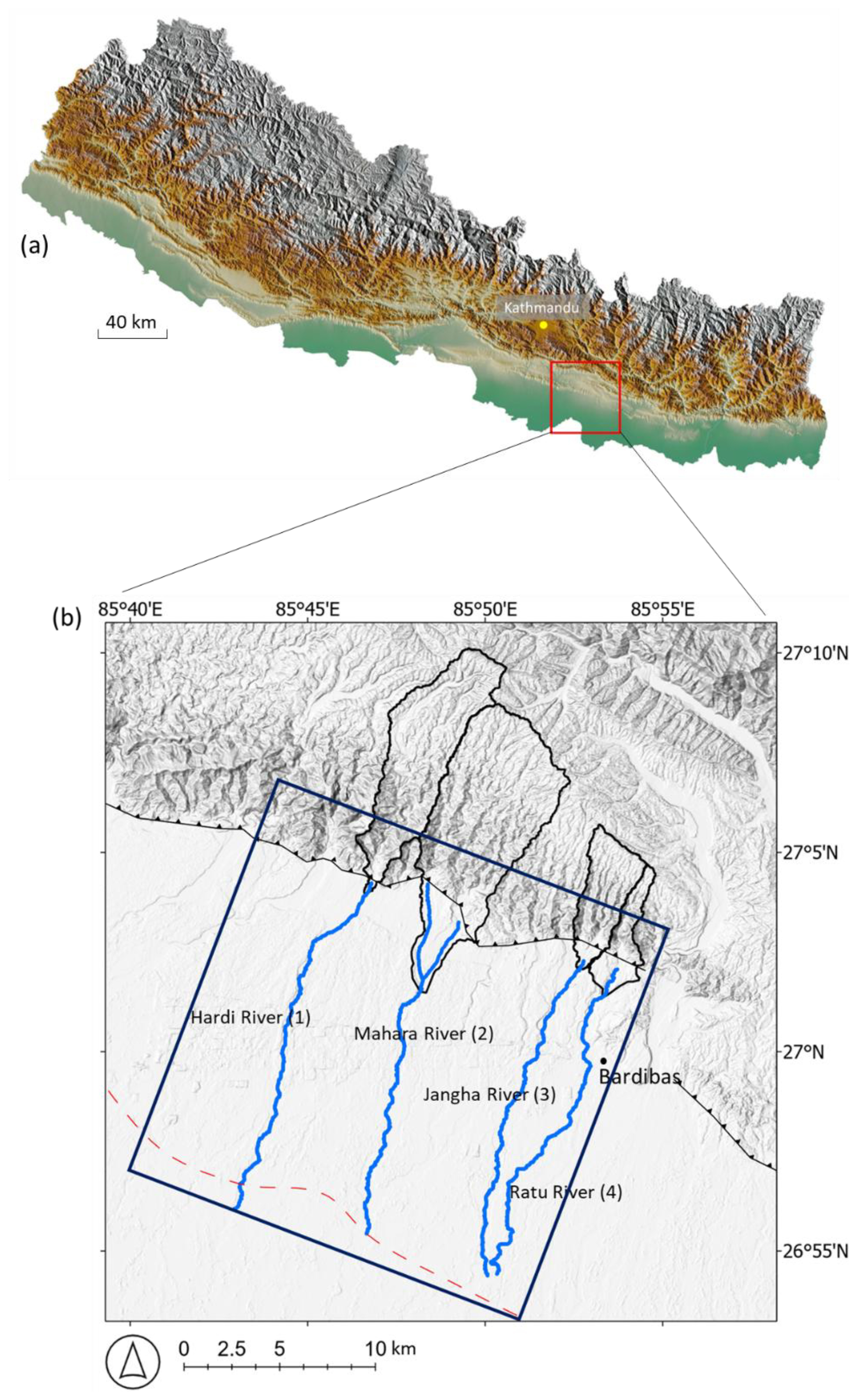
Figure 1 (a) Digital topography of Nepal showing the study area. (b) The study area focuses on four rivers (labelled 1 to 4); approximately 76 % of the surrounding land is utilized for crop growing. Rivers 1–4 within the InSAR frame (20 km² dark-blue box) are approximately 15 km in length and 300 m in width. Rivers and their catchments were generated using LSDTopoTools. Rivers were created based on the easiest flow routes along the lowest point in the channel, with a 30 m sampling rate for the river channel flow distance (Mudd et al., 2014; Clubb et al., 2014), based on a 30 m resolution DEM from http://opentopography.org (last access: 1 August 2024). Basemap data sources: ESRI World Topographic Basemap with hillshade illumination.

3 Methodology for DRTP InSAR application to dry gravel riverbeds

3.1 SAR polarimetric backscatter amplitude analysis

In our study area, the typical D50 grain size of river sediment upstream of the gravel to sand transition is around 2 cm (Dubille and Lavé, 2015; Quick et al., 2020). SAR wavelengths that are commonly utilized include the L-band (24 cm), C-band (6 cm), and X-band (3 cm). The C-band and X-band are capable of receiving backscatter from coarse gravels and cobbles with D50 around 2 cm. In this study, the C-band is chosen due to its free access to the Sentinel-1 C-band SAR data from the European Space Agency. Surface roughness is a relative term; for C-band SAR with 6 cm wavelength, if the cobble's diameter is bigger than 3 cm, which is half of the SAR wavelength, then the surface is considered rough and has a strong SAR backscattering energy (Flores-Anderson et al., 2019). The median pebble size of 2 cm is considered an intermediate rough surface for C-band SAR, resulting in moderate backscatter intensity (Fig. 2).

Figure 3 illustrates the average amplitude cover from January to May 2019 for the study area, from Sentinel-1 A/B SAR ground range detection (GRD) images in descending frame and Interferometric Wide Swath (IW) mode, with a resolution of 25 m. The SAR amplitude processing steps executed using the Sentinel-1 Toolbox include applying the orbit file, removing border noise in GRD format, eliminating thermal noise, applying radiometric calibration values, and correcting terrain geometric distortion. The image presents polarization in VV (average −12 dB along river channels) and VH (average −20 dB along river channels). Notably, the VV polarization amplitude is double that of the VH polarization, which is why VV SAR images are utilized in this study. Additionally, there is no noticeable amplitude change at the gravel–sand transition, indicating that the 6 cm C-band SAR wave does not detect the scale of roughness change from a gravel riverbed to a sandy riverbed with ripples. Since the amplitude is averaged in the dry season of 2019, the effect of soil moisture of the sandy riverbeds is unlikely to be significant. Because the SBAS-InSAR method relies on distributed backscatter, which is particularly effective in areas with diffuse scattering of stronger VV polarization, it is important to explain the backscattering type and polarization characteristics of the dry gravel riverbeds. Additionally, any application of this novel DRTP approach to more complex rivers, beyond purely ephemeral rivers, requires classifying dry gravel pixels based on SAR amplitude polarization characteristics and their statistical metrics. It is important to use SAR amplitude for classification instead of optical or multi-spectral images, as the same SAR images' phase component is used in the DRTP approach to map sediment aggradation rates.

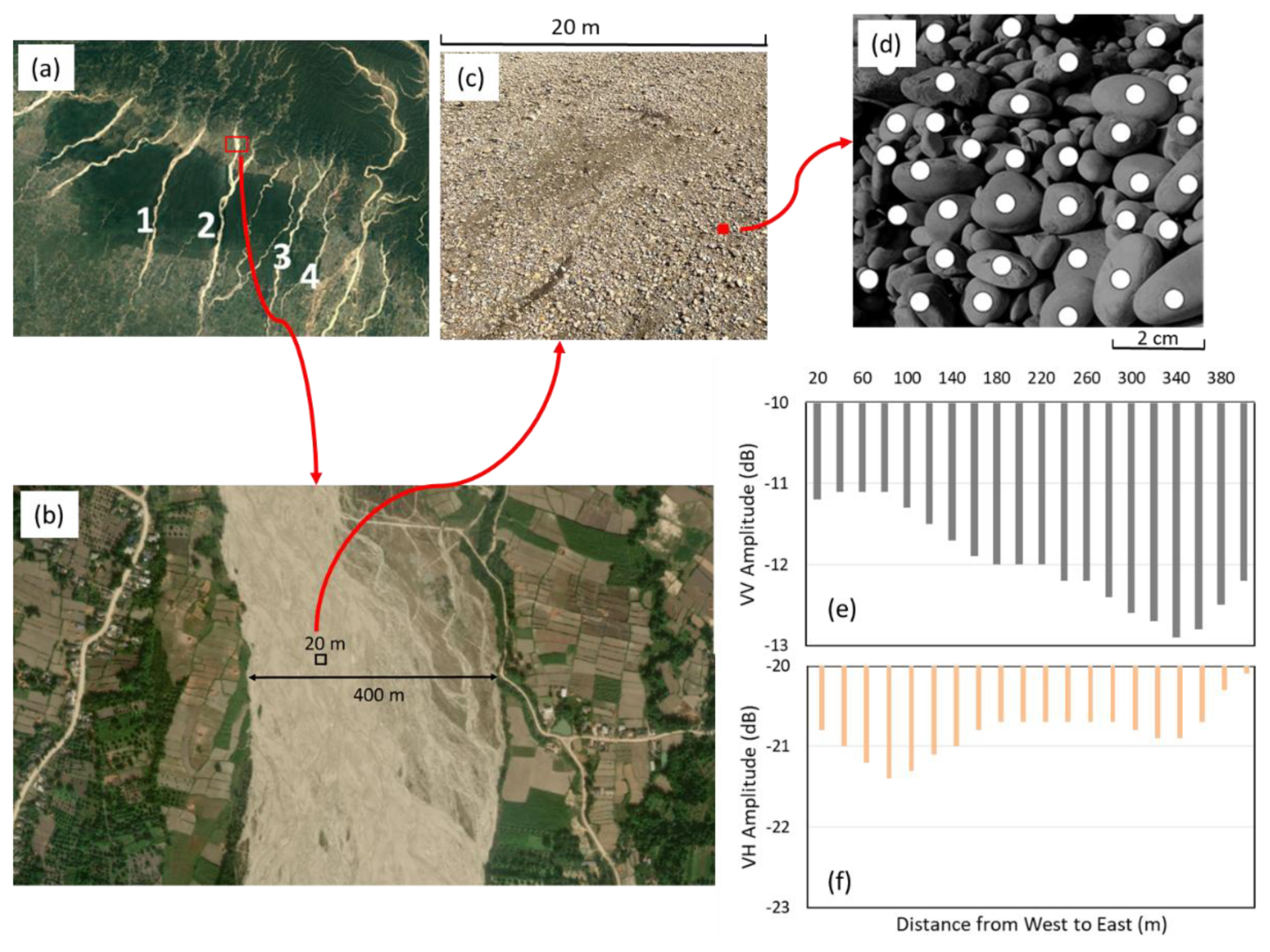
Figure 2 Illustration of the SAR diffuse scattering from a dry gravel riverbeds. The riverbeds are dominated by diffuse scattering, which is characterized by weaker signal strength but high coherence. For details of the three main types of backscattering mechanisms, please see the Supplement. This illustration demonstrates that each 20 m² InSAR mapping pixel contains tens of thousands of distributed scatters. The intensity of the SAR signal represents the sum of the distributed scatters (white dots in panel d) in that pixel. Some areas may be covered by sand bars, which exhibit lower backscatter numbers compared to areas with larger pebbles, potentially resulting in lower backscatter intensity. Histogram (e) and (f) show the distribution of VV and VH amplitude value across the 400 m wide section of the river (b) from each 20 m² pixel. The darker gravel bars in the east have relatively lower VV amplitude compared to the western gravel beds and relatively higher VH amplitude, interpreted as due to minor vegetation. The decibel (dB) scale is logarithmic, and the logarithm of a small number (less than 1) is negative. The SAR amplitude values in decibels typically range from about −25 to 0 dB for most cases. ©Microsoft.

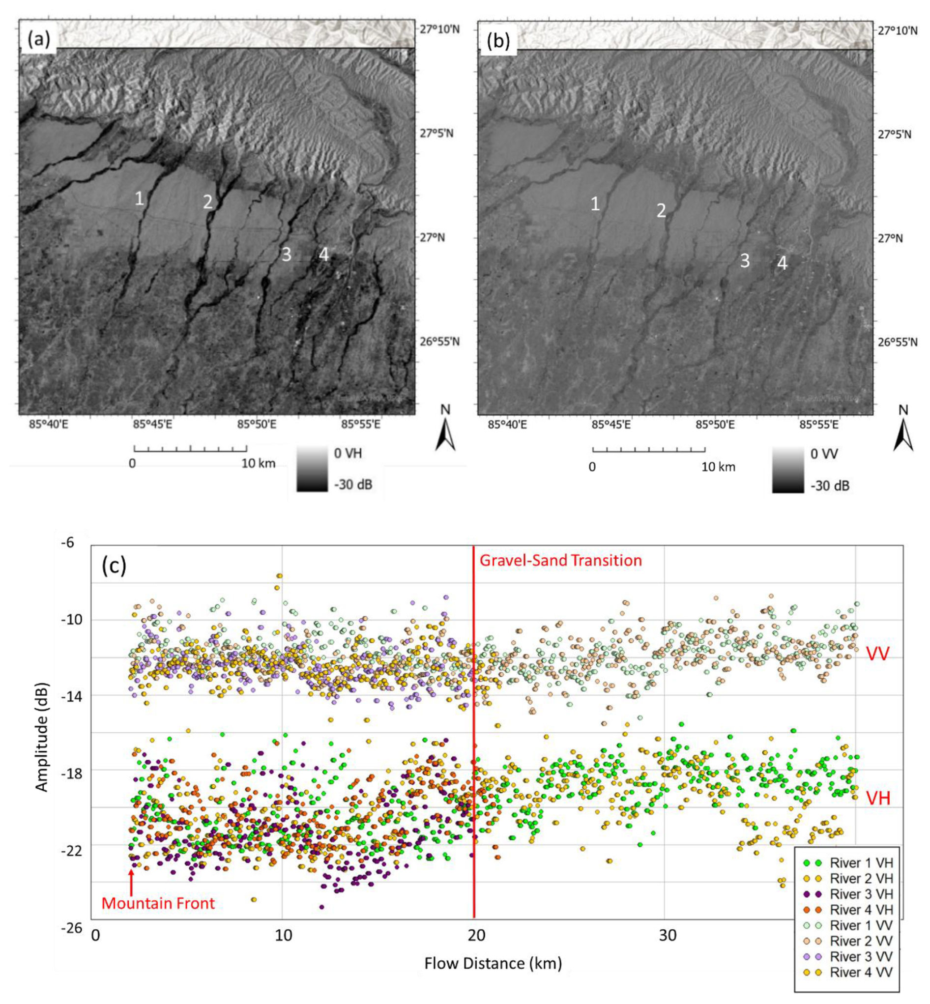
Figure 3 (a) Sentinel-1 SAR amplitude in decibels (dB) with VH (a) and VV (b) polarization, sourced from Google Earth Engine (https://developers.google.com/earth-engine/datasets/catalog/COPERNICUS_S1_GRD, last access: 1 August 2024). The mountain front is located on Fig. 1, and the gravel–sand transition is from Dubille and Lavé (2015). Sentinel-1 is dual-polarized, providing only VV and VH polarized data. The mountain regions show strong backscatter amplitude mainly due to slope orientation. Slopes that face the radar look direction can return more backscatter energy back to the satellite sensor. The forest area has higher amplitude due to strong volume backscattering, but the forest and vegetation cover areas have low coherence due to the seasonal growth change. Along the river channel VV has a higher amplitude than VH. (c) Amplitude values were plotted along river channels and all aligned to start from the mountain front, indicating that the VV polarization has double the amplitude value compared to the VH polarization. The river mountain front is the point of exit of the river from the mountains where the channel abruptly widens. There is no clear amplitude change response to roughness change at the gravel–sand transition along the rivers. The mean amplitude between the pebble and sandy sections of river 2 differs by only 1 dB (Fig. S1). This means that the 6 cm C-band SAR wave could not detect the scale of roughness change from the gravel riverbed to the sandy riverbed ripples. The SAR amplitude values are plotted here with a 30 m sampling interval. ©Google Earth.

3.2 SAR interferometric coherence analysis

To ensure the reliability of phase difference values calculated from two SAR images, a high coherence value is required (Martone et al., 2012). The coherence in interferometry of two SAR images, taken from the same location but at different times, is determined through their correlation. Coherence is a measure of the similarity between two SAR images' phase acquired at different times (Goldstein et al., 1988). High coherence of the signal between pairs of images indicates that the radar signals are consistent between the two acquisitions with high correlated phase, while low coherence means the signals are decorrelated. Coherence is an indicator of interferometric phase quality, calculated for each pixel using

$$\begin{array}{}\text{(1)}& \mathrm{coherence}={\displaystyle \frac{\left|S_{\mathrm{1}}{S}_{\mathrm{2}}^{\ast }\right|}{\sqrt{{\left|S_{\mathrm{1}}\right|}^{\mathrm{2}}{\left|S_{\mathrm{2}}\right|}^{\mathrm{2}}}}}.\end{array}$$

In this equation, S₁ and S₂ represent the complex pixel values at two different acquisition times; S^* denotes the complex conjugate operation of S (Zebker and Villasenor, 1992).

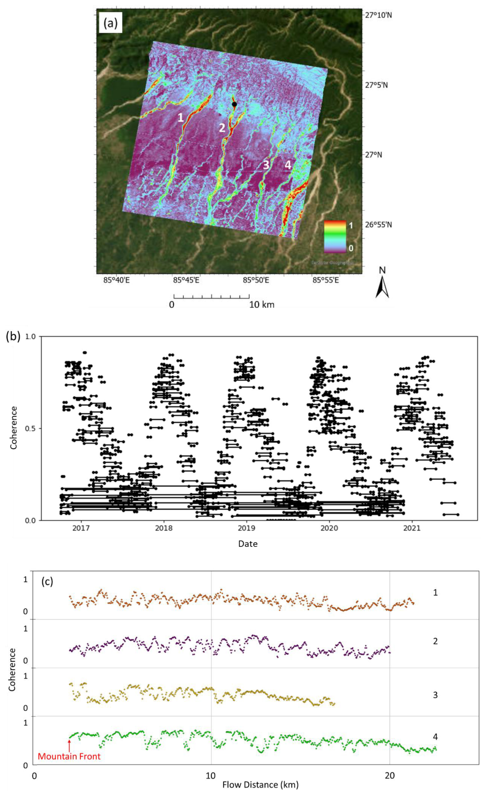
Figure 4 (a) Averaged spatial coherence map (20 m resolution) across the study area during the dry season. (b) Temporal coherence time series at the black point in panel (a) on river 2 shows seasonal variation. Within the same year, the short-time-span coherence is higher during the dry season and lower during the monsoon season, probably due to the waves on the river surface causing low coherence. The long-time-span interferograms that cross two dry seasons exhibit low coherence, likely due to sediment erosion and deposition during the migration of channels and bar forms caused by the monsoon floods. (c) Spatial coherence values were plotted along river channels, providing insights into the spatial variability with troughs at 0.3 and peaks at 0.8. The coherence troughs are typically found at the edges of the channel and vegetated sand bars, which results in fewer data points in the final InSAR results. These areas of low coherence do not show a noticeable alteration in the trend of InSAR elevation change results, but the data points in the trend are more scattered (Fig. 14). ©Google Earth.

When coherence is 1, the backscattering from two SAR images is correlated, preserving high-quality phase information. When coherence approaches 0, phase decorrelation occurs, which may result from land-cover changes and/or phase noise contamination. When two SAR images experience different atmospheric conditions than another (e.g. one SAR image acquired on a cloudy day and another SAR image acquired on a blue-sky day), the difference in the atmospheric delay can lead to phase noise that results in phase decorrelation (Yu et al., 2018). The phase recorded in a SAR image is highly sensitive to the satellite's position, especially for the topographic phase component and geometric distortion correction. The satellite's position at the time of SAR image acquisition determines the viewing angle, which is crucial information for correcting geometric distortions in SAR images. Fortunately, the Sentinel-1 satellite has well-constrained orbital control with precise orbital recording files. This means that orbital phase errors can be effectively corrected in Sentinel-1 SAR images (Filipponi, 2019).

For reliable InSAR results, coherence values should be relatively high. A commonly accepted threshold is 0.6 or higher (Cigna and Sowter, 2017). This threshold can vary depending on specific applications and the environmental conditions of the area being studied. High coherence (> 0.6) is ideal for most InSAR applications, indicating strong similarity between the two SAR images. High coherence is essential for detailed deformation analysis or for detecting subtle changes in the earth's elevation. Moderate coherence (0.3 to 0.6) is still useful, but the results may have higher uncertainty that may be adequate for broad studies where fine details are not as critical. Coherence lower than 0.3 means noise could be more prominent in the phase information. Figure 4 shows high coherence values from the 2015–2023 dry seasons, with red indicating coherence values around 0.8 along the gravel riverbeds.

The Sentinel-1 SAR Single Look Complex (SLC) interferograms were processed in full resolution (∼ 5×20 m) and then geocoded into 20 m resolution pixel size SAR interferograms (Lazecký et al., 2020). For Sentinel-1 SAR Interferometric Wide Swath (IW) acquisition mode, the single-look ground range resolution (across-track direction) is approximately 5 m, and the azimuth resolution (along-track direction) is approximately 20 m. The low multi-look value of range 4 and azimuth 1 is effective only in high-coherence areas, such as the dry-season gravel riverbeds (Fig. 4). For the rest of the study, we will quote azimuth and range in terms of pixel size, corresponding to an approximate resolution of 20 m per pixel. The SAR images with a 100 m resolution are generated by averaging neighbouring pixels; this averaging reduces speckle noise and improves the signal-to-noise ratio to effectively address low-coherence issues in cropland. This is sufficient for mapping the background basin elevation change. For 100 m resolution InSAR processing, the input consists of SAR images from all seasons, aimed at mapping the background basin elevation change signal.

3.3 SAR interferometric phase analysis

A SAR phase image is expressed in Eq. (2), and InSAR phase represents the phase change between two SAR images of the same area acquired at two different times (Flores-Anderson et al., 2019), calculated by Eq. (3). The 30 m resolution SRTM (Shuttle Radar Topography Mission) DEM (digital elevation model) from the year 2000 was used to remove the static topography phase during the interferogram calculation (Lazecký et al., 2020) (Fig. 5). The residual topographic phase is derived by subtracting the topographic phase from SRTM DEM.

$$\begin{array}{}\text{(2)}& {\displaystyle }\begin{array}{rl}& {\mathrm{phase}}_{\mathrm{1}}=\arctan {\displaystyle \frac{b_{\mathrm{1}}}{a_{\mathrm{1}}}}={\mathrm{\varnothing }}_{\mathrm{displacement}\mathrm{1}}+{\mathrm{\varnothing }}_{\mathrm{topography}\mathrm{1}}\\ & +{\mathrm{\varnothing }}_{\mathrm{flat}\mathrm{1}}+{\mathrm{\varnothing }}_{\mathrm{atmosphere}\mathrm{1}}\end{array}\text{(3)}& {\displaystyle }\mathrm{InSAR}\mathrm{phase}=\mathrm{phase}\mathrm{difference}={\mathrm{phase}}_{\mathrm{2}}-{\mathrm{phase}}_{\mathrm{1}}\end{array}$$

In Eq. (1), a₁ is the real part of the SAR image pixel value, and b₁ is the imaginary part of the SAR image pixel value. The SAR backscatter phase values are always a mixture of different source of phases, such as flat earth (earth curvature), topography, displacement, and atmospheric phase (Hanssen, 2001). After InSAR phase calculation, the residual topographic phase and line-of-sight displacement phase are the dominant phases in our cases (Gaber et al., 2017). There are two multi-temporal InSAR techniques: permanent scatterers (PSs) and SBAS. The PS-InSAR method estimates the residual topographic phase by using its linear relationship with the perpendicular baseline. This technique models and eliminates residual topographic phases by comparing phase observations across images that have varying baselines, thereby effectively removing the residual topographic phase (Ferretti et al., 2001; Hooper et al., 2004). The SBAS-InSAR method relies on the accuracy of the DEM used to remove the topographic phase. If the DEM is outdated, it will include the residual topographic phase mixed with the line-of-sight (LOS) motion phase as input for SBAS inversion, leading to higher uncertainty in the LOS displacement results (Berardino et al., 2002; Morishita et al., 2020). The PS-InSAR method relies on persistent backscatters, making it most effective in urban areas with strong double-bounce scattering. Conversely, the SBAS-InSAR method relies on distributed backscatters (one phase value from the sum of a pixel's backscatters), particularly effective in areas with lower coherence and mixed backscatter mechanisms types (diffuse scattering, volume scattering, and double bounce). In this study, we have selected the SBAS-InSAR method as it is better suited for rural areas with diffuse scattering (Fig. 2).

The short-time-span interferograms refer to time pairs that are over shorter intervals than 90 d, as InSAR coherence typically exhibits seasonal variations in the study area. Long-time-span interferograms span 90 to 360 d, designed to bridge network gaps across different seasons. The short-time-span interferogram from the dry season maintains good coherence, with an average value of 0.6 along dry riverbeds, ensuring reliable interferometric phase calculations (Fig. 6); this would be expected if there is little disturbance of the riverbeds between the time pairs. The interferograms are unwrapped using a statistical cost approach with the SNAPHU software (Chen and Zebker, 2002). The long-time-span interferograms exhibit low coherence, probably linked to sediment erosion and deposition during the migration of channels and bar forms during the monsoon floods (Fig. 7). These decorrelated phases are insufficient for obtaining reliable interferograms, and the long-time-span interferograms are excluded from the 20 m resolution SBAS-InSAR processing.

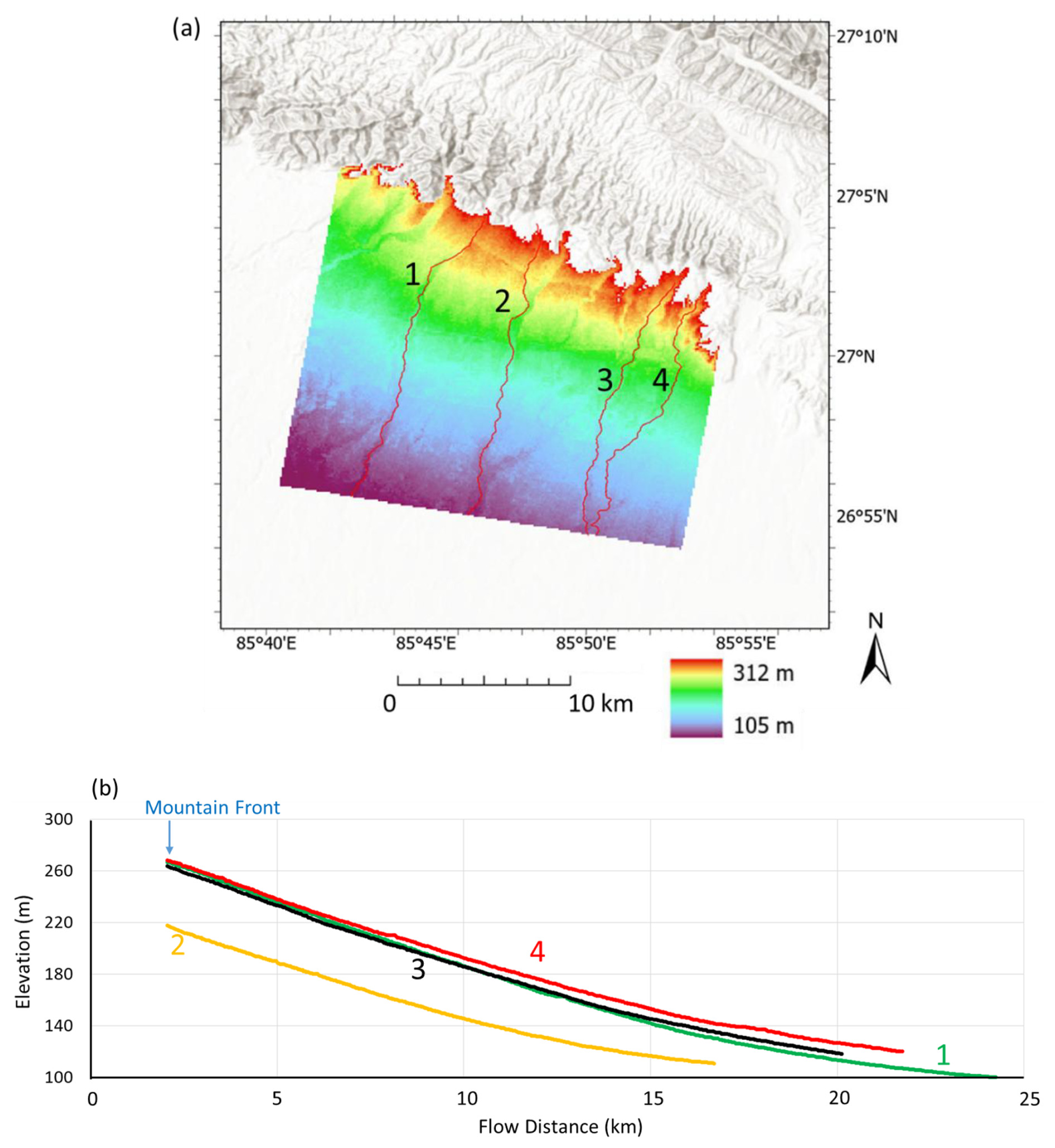
Figure 5 (a) The 30 m resolution SRTM DEM (Esri). The terrain shows a gradient in the topographic phase values. This DEM was used to remove the static topography phase during the interferogram calculation process, which is carried out using the GAMMA software as implemented by the LiCSAR (Lazecký et al., 2020). The residual topographic phase is derived by subtracting the topographic phase from the year 2000 SRTM DEM. (b) River long profiles showing no obvious evidence of knick points. From the mountain front to the gravel–sand transition, the elevation of the river channel decreases by around 150 m. The exact season when the DEM data were collected is unknown. Consequently, the elevation data along the river channel may represent the water surface elevation rather than the dry riverbed elevation.

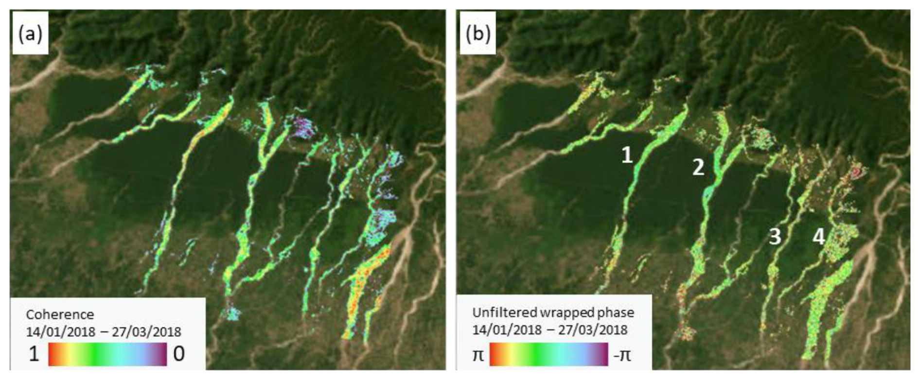
Figure 6 Short-time-span interferogram coherence (a) and unfiltered wrapped phase (b) (20 m resolution, 0.2 coherence masked, acquired on dates 14 January and 27 March 2018, 72 d). Phase changes between adjacent pixels are relatively small and continuous. The continuous shifts in colour along the river shows a smooth, low-phase-gradient feature that contributes to a more accurate phase unwrapped interferogram. ©Google Earth.

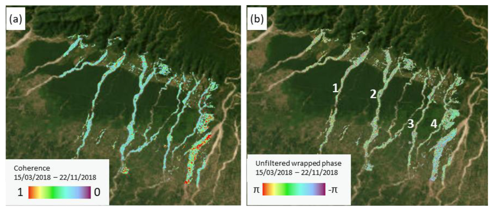
Figure 7 Long-time-span interferogram coherence (a) and unfiltered wrapped phase (b) (20 m resolution, 0.2 coherence masked, acquired on dates 15 March and 22 November 2018, 252 d). Based on coherence data, the months from November to March are identified as the driest in the study area. Most regions shown in blue in panel (a) display coherence values below 0.3, indicating that they are insufficient for obtaining reliable interferometric phase. Areas of high coherence on the eastern side are depicted in red in panel (a) and correspond to an embanked, inactive gravel riverbed. ©Google Earth.

3.4 SAR interferogram network for SBAS-InSAR processing

The SBAS-InSAR processing method was developed in the early 2000s by Berardino et al. (2002) to invert the temporal surface displacement. It is a linear inversion method, and in this study we implement the SBAS-InSAR method by using LiCSBAS software (Morishita et al., 2020). The atmospheric noise correction is applied by using the GACOS data (Yu et al., 2018). The success of this method heavily relies on the quality and availability of abundant InSAR images.

We processed two SBAS-InSAR datasets aimed at monitoring changes in both channel and floodplain elevation changes: 20 m resolution data specific to the dry season (October–May) from year 2016 to 2021 that targeted the channels (Fig. 8) and 100 m resolution covering all seasons from year 2016 to 2021 aimed at monitoring the floodplains (Fig. 9). Reference point selection is another important factor, due to having limited coverage area, and a relatively stable reference point for resolution processing is important. We choose to use a reference point at an airport (26.93° N, 85.86° E) in an embanked inactive gravel riverbed, marked in Fig. 11.

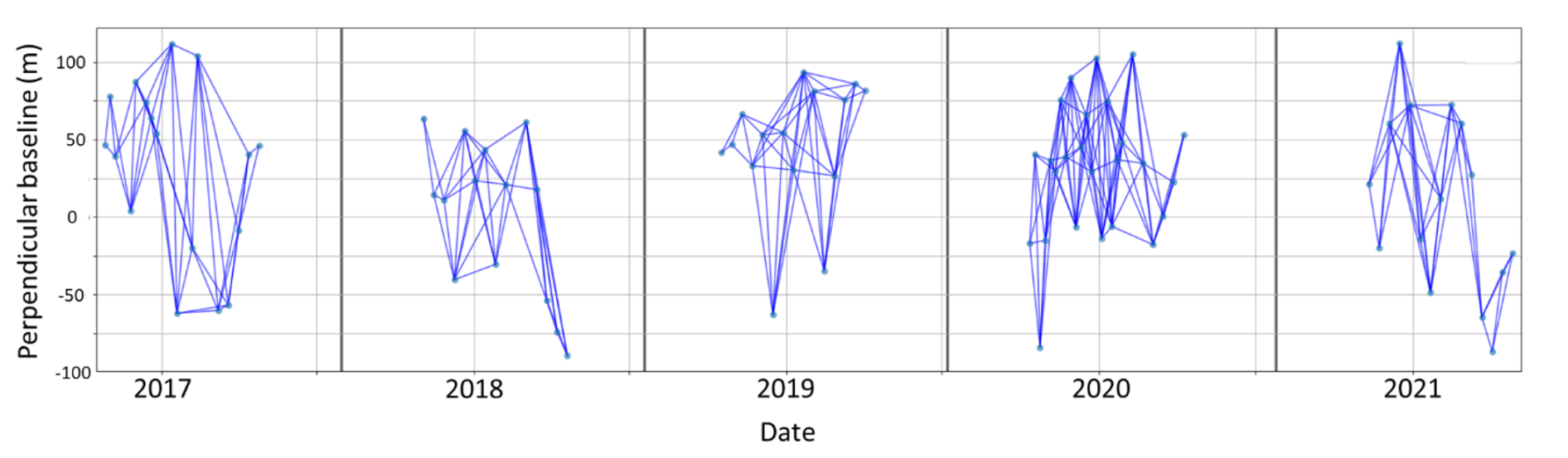
Figure 8 A network of 20 m resolution interferograms. The y axis is the perpendicular baseline versus acquisition dates on the x axis. The perpendicular baseline is the distance between the satellite orbits when the satellite revisits the same location. Each blue line connects two SAR images for calculating interferograms. Each dark-grey vertical line indicates a gap in the network. We are leveraging the residual topographic phase, so the gaps in the network are filled by the differential residual topographic phase. Maintaining a consistent range of perpendicular baselines within each network segment is crucial for preserving the sensitivity to topographic phase changes (Fattahi and Amelung, 2013).

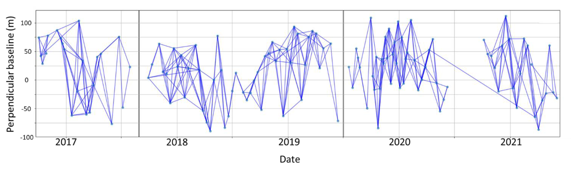
Figure 9 A network of 100 m resolution interferograms for mapping the basin cropland. Each blue line connects two SAR images for calculating interferograms. Each dark-grey vertical line indicates a gap in the network. This is based on the traditional LOS displacement phase, so the gaps are filled by the high-quality long-time-span interferogram. It is important to highlight that long-time-span interferograms with a 20 m resolution are not effective for analysing gravel riverbeds. The 100 m resolution long-time-span interferogram is sufficient for cropland mapping, offering a practical solution to bridge the network gaps. There are two small time gaps in the 100 m resolution network, linked by linear fit through LiCSBAS processing. Due to the gaps being relatively small, there is an insignificant effect on the subsidence time-series analysis in Sect. 5.

3.5 SBAS-InSAR processing based on differential residual topographic phase

Along dry gravel riverbeds, the phase change sensitivity to the perpendicular baseline (red and black phase profiles in Fig. 10) indicates that the phase is dominated by the residual topographic phase. A previous study (Du et al., 2016) demonstrated that utilizing the multi-temporal InSAR technique, which is based on stacked interferograms, enhances the accuracy of the calculations of the residual topographic phase. They also observed that the sensitivity of the residual topographic phase is influenced by the overall range of perpendicular baselines within the entire network of interferograms for each time segment rather than the baseline of any single interferogram in the stacked calculation. The stability of residual topographic phase estimation is maintained, irrespective of the way in which the selected short-baseline interferograms are linked (Du et al., 2016; Fattahi and Amelung, 2016).

The residual topographic phase has traditionally been treated as noise to be removed for accurate line-of-sight displacement phase processing. However, our study reveals that the dry gravel riverbeds at the Himalayan mountain front provide a favourable geomorphic setting for retrieving high-quality residual topographic phases. This is attributed to their annual bedload sedimentation and the strong diffuse scattering caused by the gravel. Additionally, the Sentinel-1 SAR data, with their 10-year span, 12 d revisit frequency, and well-constrained orbital tube, offer a rich dataset for recording these accurate residual topographic phases.

In our study, we use the SBAS-InSAR technique to invert the differential residual topographic phase to elevation change rates. The inversion of the DRTP network for the estimated phase history is implemented in LiCSBAS software (Morishita et al., 2020) using the NSBAS technique, which assumes a linear deformation model. The phase history's effect is predominantly influenced by DRTP along the river channels, as expressed in Eq. (7). The variations of baseline resulting in small jumps within the same year during the dry season are caused by the topographic phase ambiguity. We maintained the perpendicular baseline within a range of ±100 m because the majority of the interferograms fall within this range. The offset between the different years' residual topographic phase includes the combination of topographic phase ambiguity and phase changes linked to changes in the height of the sediment. It is important to note that the differential topographic phase caused by river sediment aggradation is larger than the variations caused by the topographic phase ambiguity. The final elevation change rates are calculated from the residual topographic phase history based on Eq. (7). The DRTP approach enables tracking of elevation changes even in cases of land-cover change, where coherence is lost, preventing the retrieval of the line-of-sight displacement phase.

To summarize, the SBAS-InSAR processing based on differential residual topographic phase relies on several assumptions. (1) The residual topographic phase is the predominant phase value along the dry riverbeds, unaffected by noise and LOS displacement phase. To support this assumption, the background LOS displacement signal must be analysed and separated. The time-series mapping of the basin background indicates that the LOS displacement remains flat during the dry season (Fig. 17). Therefore, we assume that the phase observed along the dry gravel riverbeds is primarily from the residual topographic phase. Additionally, we examined the unwrapped phase profile along the river and its sensitivity to the perpendicular baseline, which demonstrates a positive linear relationship between topographic phase sensitivity and the perpendicular baseline (Fig. 10). (2) The network connectivity of each acquisition time results in similar topographic phase ambiguity (Fig. 16), as indicated by relatively flat time series within the same year. (3) We account for variations in the scaling factor by calculating the average perpendicular baselines for the five different connected networks as 52.2, 52.8, 49.5, 48.4, and 50.4 m (Fig. 8). Consequently, the ratios of $B_{\perp \mathrm{2}}/B_{\perp \mathrm{1}}$ are 1.01, 0.94, 0.94, and 1.04. To quantify the uncertainty percentage caused by these ratios, we conducted forward modelling (see the Supplement) and observed their effect on the elevation change ratios to be +2 %, −12 %, −12 %, and +8 %. Therefore, we conclude that the impact of the scaling factor on the final result's uncertainty percentage falls within the range of +8 % to −12 % (Fig. 14).

$$\begin{array}{}\text{(4)}& {\displaystyle }{\mathrm{\varnothing }}_{\mathrm{residual}\mathrm{\_}\mathrm{topo}\mathrm{1}}={\displaystyle \frac{\mathrm{4}\mathit{\pi }{B}_{\perp \mathrm{1}}}{\mathit{\lambda }}}{\displaystyle \frac{H_{\mathrm{1}}-H_{\mathrm{dem}}}{R_{\mathrm{1}}\sin \left(\mathit{\theta }\right)}}\text{(5)}& {\displaystyle }{\mathrm{\varnothing }}_{\mathrm{residual}\mathrm{\_}\mathrm{topo}\mathrm{2}}={\displaystyle \frac{\mathrm{4}\mathit{\pi }{B}_{\perp \mathrm{2}}}{\mathit{\lambda }}}{\displaystyle \frac{H_{\mathrm{2}}-H_{\mathrm{dem}}}{R_{\mathrm{2}}\sin \left(\mathit{\theta }\right)}}\text{(6)}& {\displaystyle }\begin{array}{rl}& \mathrm{\Delta }{\mathrm{\varnothing }}_{\mathrm{residual}\mathrm{\_}\mathrm{topo}}={\displaystyle \frac{\mathrm{4}\mathit{\pi }}{\mathit{\lambda }\sin \left(\mathit{\theta }\right)}}\\ & \left({\displaystyle \frac{B_{\perp \mathrm{2}}\left(H_{\mathrm{2}}-H_{\mathrm{dem}}\right)}{R_{\mathrm{2}}}}-{\displaystyle \frac{B_{\perp \mathrm{1}}\left(H_{\mathrm{1}}-H_{\mathrm{dem}}\right)}{R_{\mathrm{1}}}}\right)\end{array}\end{array}$$

After applying the parallel-ray approximation, the mathematical relationship between residual topographic phase Φ_{residual_topo} and height (H) can be written in Eqs. (4) and (5); H₁ is the height at time 1, H₂ is the height at time 2, and H_dem is the height of the DEM used to remove the topographic phase (Fattahi and Amelung, 2013; Pepe and Calò, 2017). By combining Eqs. (4) and (5), we are able to derive Eq. (6), where B_⊥ is the perpendicular baseline, λ is the SAR wavelength, Θ is the satellite SAR acquisition average incident angle, and R is the distance between satellite and earth surface (Fig. S2). In Eq. (6), the parameter R is approximately 700 km. Since centimetre-level surface displacements are negligible in comparison to R, it is reasonable to assume that R₁=R₂. Then we could write Eq. (6) as follows:

$$\begin{array}{}\text{(7)}& \begin{array}{rl}& \mathrm{\Delta }{\mathrm{\varnothing }}_{\mathrm{residual}\mathrm{\_}\mathrm{topo}}={\displaystyle \frac{\mathrm{4}\mathit{\pi }{B}_{\perp \mathrm{1}}}{\mathit{\lambda }\sin \left(\mathit{\theta }\right)R}}\\ & \left({\displaystyle \frac{B_{\perp \mathrm{2}}}{B_{\perp \mathrm{1}}}}\left(H_{\mathrm{2}}-H_{\mathrm{dem}}\right)-\left(H_{\mathrm{1}}-H_{\mathrm{dem}}\right)\right).\end{array}\end{array}$$

The key component in Eq. (7) is the ratio $B_{\perp \mathrm{2}}/B_{\perp \mathrm{1}}$, which influences the percentage of the elevation change results. This equation is novel because it not only accounts for the scaling factor caused by the topographic phase ambiguity but also, for the first time, demonstrates that elevation change can be mapped through DRTP. Ideally, if $B_{\perp \mathrm{2}}/B_{\perp \mathrm{1}}=\mathrm{1}$, we would achieve the perfect elevation change results. During data processing, the goal is to balance the number of input interferograms while keeping the ratio of $B_{\perp \mathrm{2}}/B_{\perp \mathrm{1}}$ as close to 1 as possible.

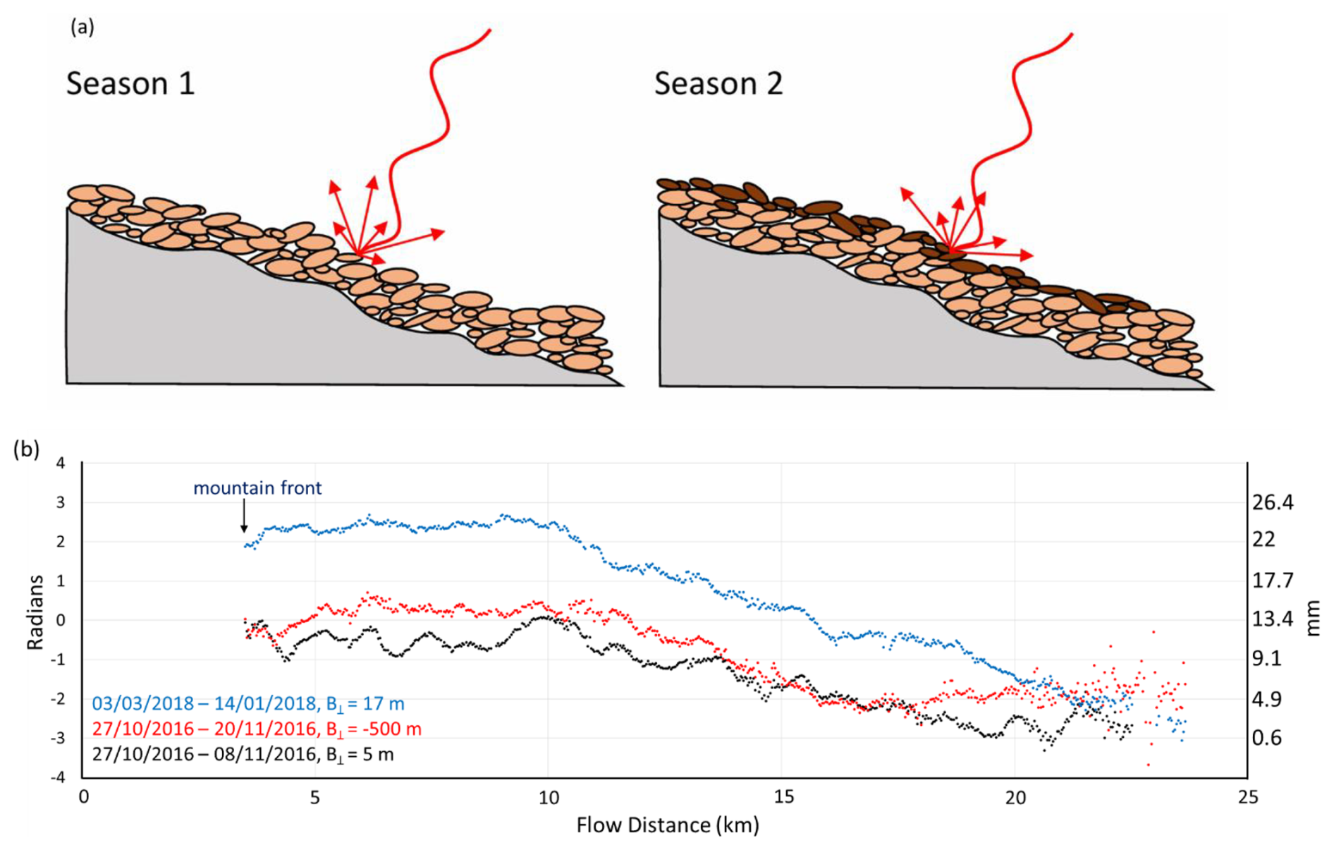
Figure 10 (a) Illustration of the annual increase in dry gravel riverbed topographic elevation due to sediment aggradation. Dark-brown pebbles show accumulation in season 2. (b) Changes in the residual topographic phase along river 2, influenced by sediment aggradation and perpendicular baseline variations. The filtered unwrapped phase values are plotted along river 2, comparing residual topographic phase observations with different perpendicular baselines from the same year (black and red curves), as well as the residual topographic differences between 2016 and 2018 with a similar perpendicular baseline (blue and black curves). From the same year, the large baseline (red) measured topographic phases are higher than smaller baseline measurements (black). This indicates that a larger perpendicular baseline increases the sensitivity of the interferometric phase to topographic elevation. Comparing different years, the year 2018 (blue) has higher residual topographic phase values due to sediment aggradation.

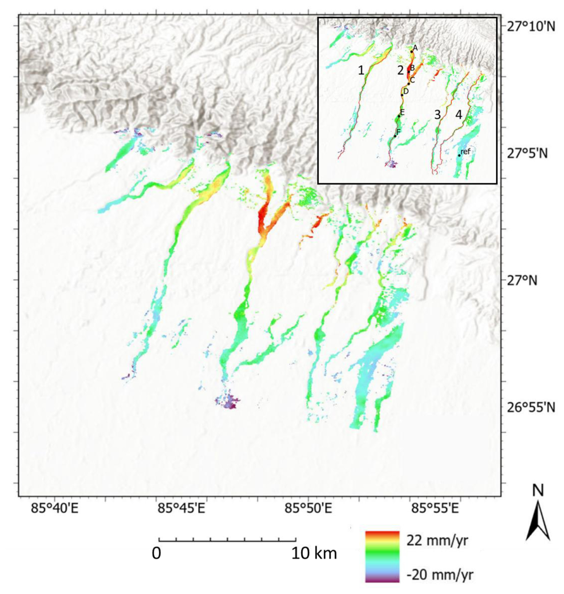
Figure 11 Spatial distribution of elevation change from 2016–2021 (20 m resolution) for dry gravel riverbeds. An inset within the figure provides detailed annotations. The results show the positive elevation change broadly decreasing with distance from the mountain front. The 20 m resolution SAR dataset focuses solely on mapping the rate of elevation change of dry river channels based on the residual topographic phase. Basemap data sources: ESRI World Topographic Basemap with hillshade illumination.

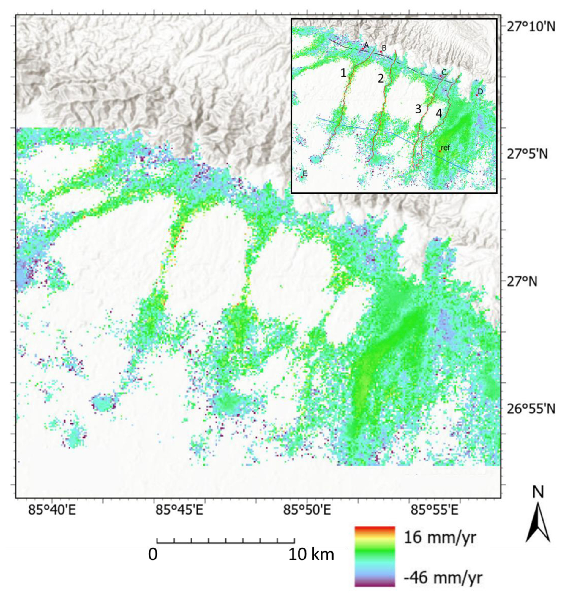
Figure 12 Spatial distribution of LOS displacement from 2016–2021 (100 m resolution) for the basin. An inset within the figure provides detailed annotations. This figure shows the negative elevation change in the basin. Due to the vegetation decorrelation effects, the results are sparse. The villages have denser pixels, attributable to the strong double-bounce backscattering caused by houses. The 100 m resolution data are used only for mapping the basin based on the LOS displacement phase. For the detailed LiCSBAS processing implementation based on LOS displacement phase, please see the Supplement. At the river, the data are considered unreliable due to contamination from monsoon season river water. Basemap data sources: ESRI World Topographic Basemap with hillshade illumination.

3.6 SBAS phase velocity standard deviation

The phase-change-related elevation change is sensitive to sub-wavelength elevation change, which is the basis for the InSAR technique. This is based on the condition of reliable phase differences as input for the data processing. Accurately measuring the phase difference is crucial, and efforts should be made to minimize noise. Typically, this phase is the LOS displacement phase. However, in our 20 m resolution processing for dry gravel riverbeds, it is based on the differential residual topographic phase. Figure 13 displays the standard deviation of the final InSAR velocity. A higher standard deviation indicates greater variability and noise in the measured velocity. The standard deviation is primarily influenced by the quality of the unwrapped interferogram used to calculate the final InSAR velocity. The velocity standard deviation is calculated based on a bootstrapping approach, which uses the cumulative displacement data and repeated bootstrap sampling from original cumulative displacement data and then calculates the velocity. Note that the standard deviation might be underestimated if the network is not fully connected, due to the temporal constraint in the small baseline inversion (Morishita et al., 2020).

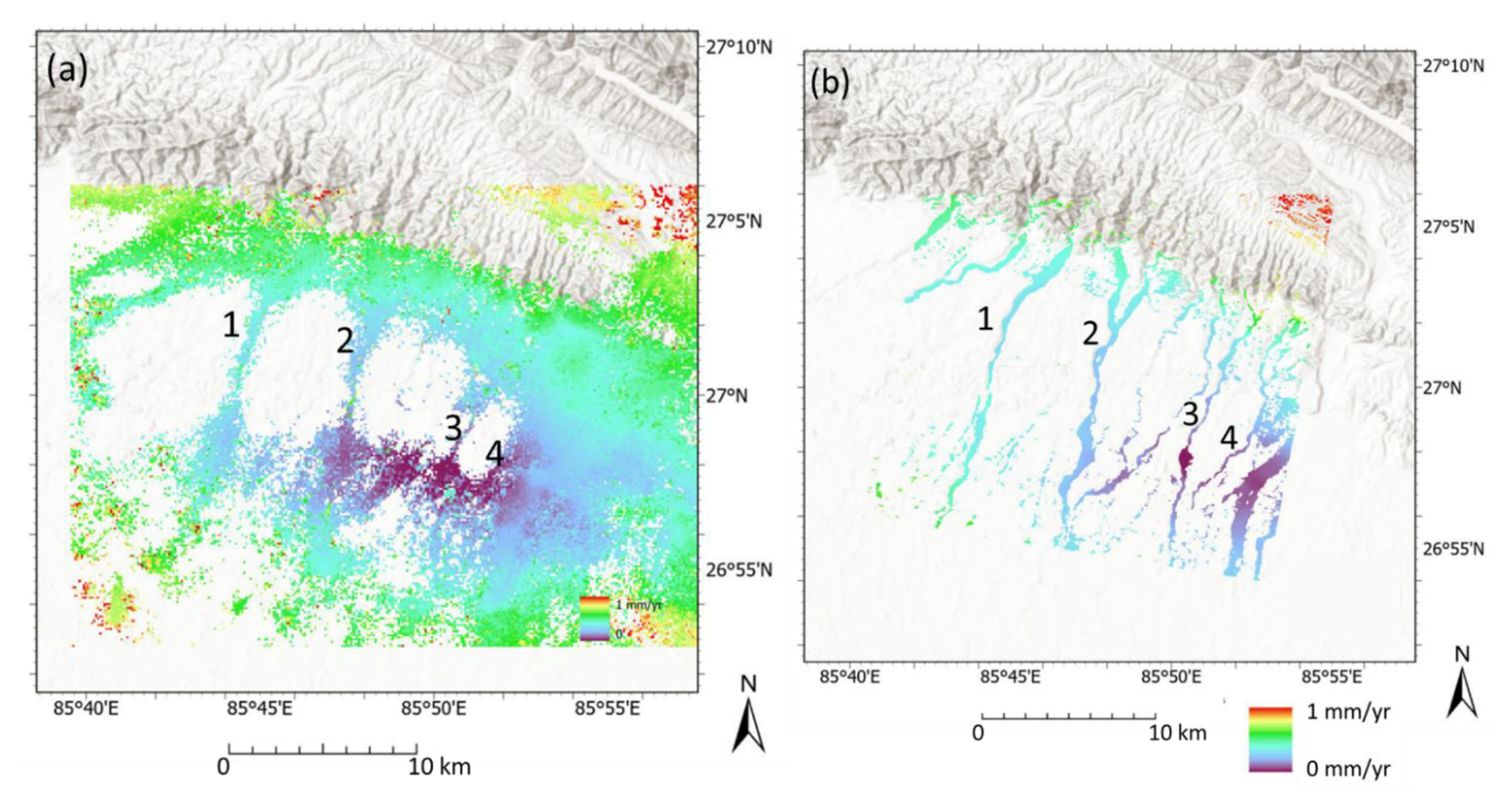
Figure 13 Standard deviation of the InSAR velocity for 100 m resolution (a) and 20 m resolution (b). The standard deviation ranges from 0–1 mm yr⁻¹. The standard deviation measures the variability and noise in the measured velocity trend, which is the linear fit of the time-series points. The calculation of the velocity standard deviation assumes that all input pixel values from the InSAR images are reliable. For the 100 m resolution InSAR results at river channels, despite showing a positive elevation trend, the values are considered unreliable due to high noise contamination. This unreliability comes from noise in the InSAR images taken during the monsoon season. Consequently, the 100 m resolution InSAR results are solely employed for mapping basin elevation changes, while the 20 m resolution InSAR results are used to map changes in river channel elevation. Basemap data sources: ESRI World Topographic Basemap with hillshade illumination.

4 Results

4.1 InSAR signals of fluvial elevation change

A spatial distribution map from the 20 m InSAR result analysis along rivers 1–4 indicates a positive elevation change along the river channels. Near the mountain front, the upstream section of the rivers experiences a positive elevation change of approximately 20 mm from one dry winter season to the next (i.e. 20 mm yr⁻¹), which gradually decreases with distance from the mountain front (Fig. 14). Initially, all rivers exhibit a decline in the rate of elevation change that ends at the forest's edge. The elevation change progressively declines through the forest to a minimum of about 5 mm yr⁻¹. Beyond this, the elevation change varies between 0 and 5 mm yr⁻¹ until it reaches the gravel–sand transition, where it begins to fall below zero (Fig. S4).

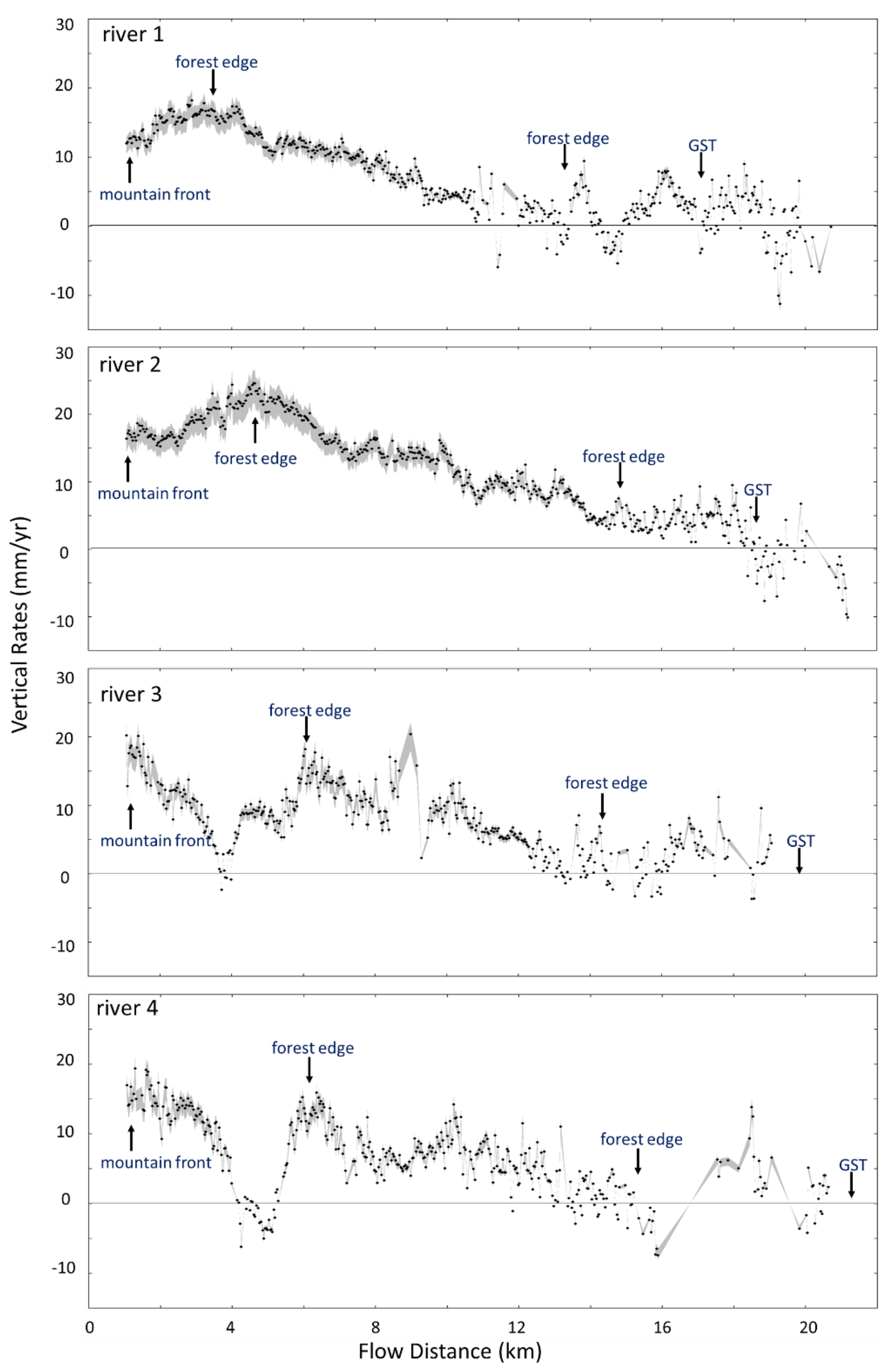
Figure 14 Vertical elevation change rates from 2016 to 2021 along each river. The rates are derived from the DRTP SBAS-InSAR results. River 1 peaks at 15 mm yr⁻¹, river 2 at 25 mm yr⁻¹, river 3 at 20 mm yr⁻¹, and river 4 at 15 mm yr⁻¹. The uncertainty range due to the scaling factor effect, shaded in grey, spans from −12 % to +8 %. The plot uses a vertical exaggeration of 250 000, meaning the vertical scale is magnified 250 000 times relative to the horizontal. Each dot represents elevation change rates over a 20 m² pixel along the dry riverbeds.

4.2 InSAR signals of floodplain elevation change

A spatial distribution map of the 100 m resolution InSAR analysis in the basin indicates a negative elevation change (i.e. subsidence) of the surrounding floodplains. Figure 15 displays two plotted cross-sections: one situated north of the forest (marked with a black-coloured dot) and the other located south of the forest (marked with a blue-coloured dot). Both transects show negative elevation change. The southern (blue) transect has values between 0 and −15 mm yr⁻¹, while the northern (black) transect has values between −5 and −25 mm yr⁻¹. The elevation changes along river channels are excluded due to the high noise contamination from SAR images captured during the monsoon season.

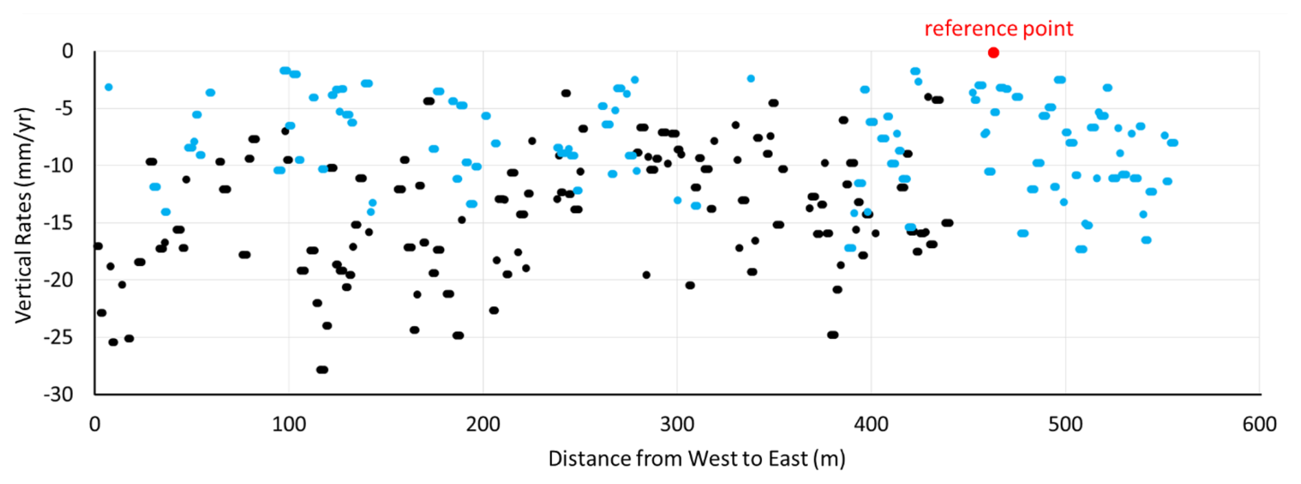
Figure 15 Basin transects of the InSAR analysis (northern black and southern blue lines in Fig. 12) indicate high heterogeneity in the distribution of subsidence across the basin, potentially caused by water extraction. Values from cropland and villages are shown in the transect plot, while elevation changes along the riverbeds affected by monsoon season interferograms are excluded. The reference point for InSAR processing, located near the blue transect, is projected onto the plot and marked with a red dot.

5 Time-series analysis of elevation change

Based on the time-series pattern, we can interpret the cause of the elevation change. We chose six different locations (dots in Fig. 11) that characterize the typical signal pattern of the time series along rivers with a 20 m resolution. The locations analysed in further detail are located along river 2, with a minimum coherence value of 0.5 and a maximum velocity standard deviation of 0.5 mm yr⁻¹ (Fig. 12). Based on the time series, the characteristics are similar, showing minor fluctuations around their average values, followed by an increase in elevation after the monsoon (Fig. 16). These fluctuations are during the dry period where no water is discharged through these channels. The reason for the fluctuation (Fig. 16) could be a mixture of noise and the diversity of perpendicular baselines, which causes different degrees of topographic sensitivity. However, the fluctuation is within a 5 mm range and does not cause a dramatic change in vertical displacement measurements; i.e. it is still within the range of a flat feature. We interpret that the inter-seasonal displacements shown in the time series are predominantly due to the differential residual topography phase caused by sediment aggradation along river 2.

We chose five different locations (dots in Fig. 12) that characterize the typical signal pattern of the time series in the floodplain areas with 100 m resolution. The locations are spread in high-coherence pixels in cropland and villages, with a minimum coherence value of 0.4 and a maximum velocity standard deviation of 0.5 mm yr⁻¹. Based on the time-series patterns observed at five locations in the basin, the characteristics are similar, with a meaningful subsiding trend between each point during the crop growing season (Fig. 17).

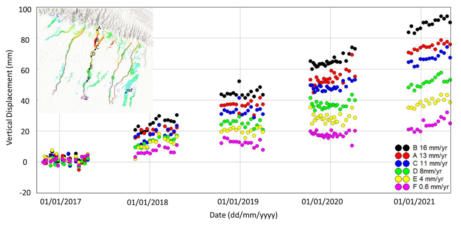
Figure 16 The SBAS-InSAR (20 m resolution) time series along river 2 shows positive elevation changes. The June to September gap corresponds to the monsoon season. The inter-seasonal displacements shown in the time series are predominantly due to sediment aggradation. The fluctuations in the measurement points during the dry period could be due to a combination of noise and varying perpendicular baselines, which cause variations in topographic phase ambiguity. Basemap data sources: ESRI World Topographic Basemap with hillshade illumination.

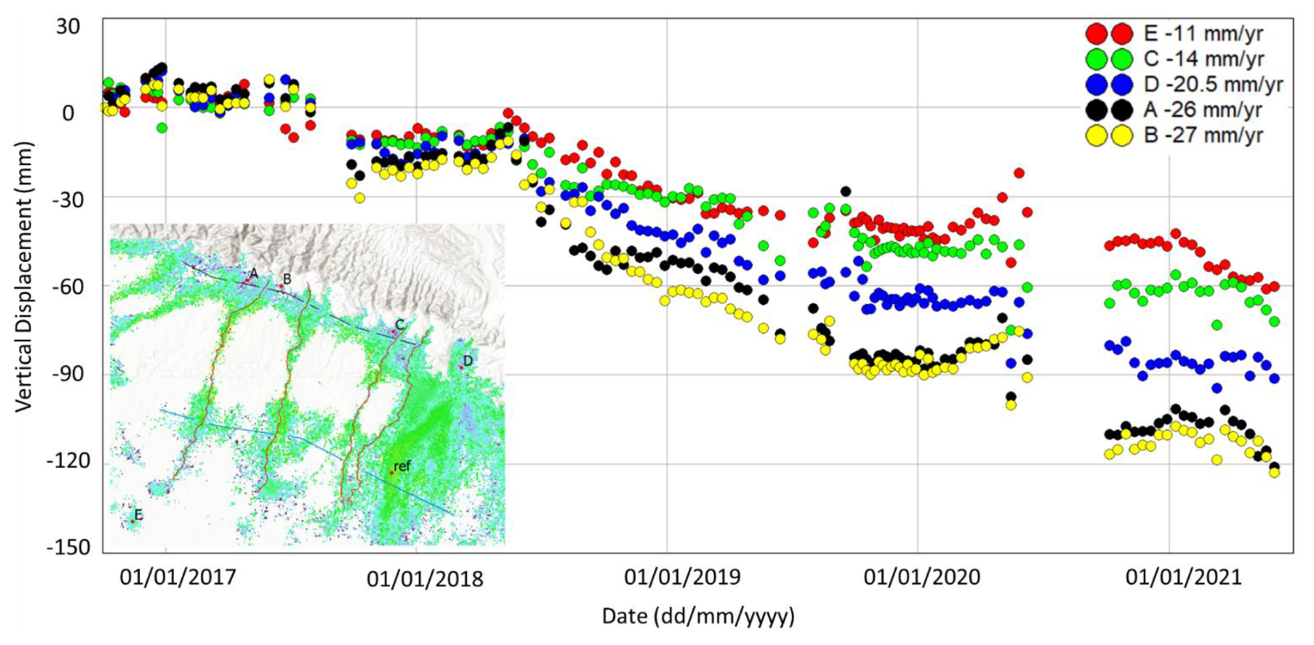
Figure 17 The SBAS-InSAR (100 m resolution) time series in the floodplain shows a consistent pattern of negative elevation change, indicative of subsidence at each observed location. To ensure accuracy, there are no gaps in the network, which is connected by both short- and long-time-span interferograms. Basemap data sources: ESRI World Topographic Basemap with hillshade illumination.

6 Discussion

6.1 Uncertainties generated by working in active river settings

To map the river aggradation rate, satellite DEMs offer metre-scale accuracy, while airborne lidar can achieve accuracies within tens of centimetres. Two-pass InSAR (DInSAR) typically maps elevation changes with an accuracy of up to a few centimetres, but multi-temporal InSAR processing can improve the accuracy to millimetre scale (Massonnet and Feigl, 1998). These are general ranges, and the actual accuracy will vary between projects. The key to effectively using the residual topographic phase for mapping elevation changes rests in confirming whether the feature of elevation change supports the precise measurement of the topographic phase. In our study, we observed that the four rivers completely dry out during the dry season, leaving the surface undisturbed. Most importantly, the 100 m resolution basin mapping indicates a minimal LOS displacement phase during the dry season (Fig. 17). This observation is crucial as it ensures that the dominant phase is due to the residual topographic phase rather than the LOS displacement phase. In our study area, the LOS displacement phase difference is positive, while the differential residual topography phase causes a negative phase difference. They contribute in opposite directions to the differential phase measurement. Therefore, it is crucial to have a predominantly topographic phase mapping time period, with the minimal LOS displacement phase component mixed in the observed phase.

We have a 7-month dry-season window to acquire abundant SAR images for mapping the topographic phase. Maintaining a sufficient number of interferograms for SBAS-InSAR analysis input is important to ensure reliable and stable results. Using data from only 2 years leads to high uncertainties in the results. Therefore, we have incorporated 5 years of Sentinel-1 data, with a minimum of 15 interferograms each year. In our study area, the low phase gradients facilitate accurate phase unwrapping. Additionally, conditions such as low atmospheric phase noise during the dry season and the absence of layover, shadow, and foreshortening geometry distortions contribute favourably to get the accurate topographic phase value.

The sensitivity of the topographic phase has a linear relationship with the perpendicular baseline. Therefore, maintaining a consistent range of perpendicular baselines within each network segment is essential to ensure a consistent sensitivity of topographic phase measurement (Fattahi and Amelung, 2013). Sentinel-1's precise and stable orbital tube plays a crucial role in baseline control for this study. We have maintained the perpendicular baseline within a range of ±100 m because the majority of the interferogram is within this baseline range (Fig. 8). As outlined in Eq. (7), the LOS displacement between each year must also be minimal to support the assumption that the scaling factor is 1. It is important to note that the scaling factor does not influence the trend of elevation change.

6.2 Validation of the DRTP SBAS-InSAR method in active river settings

Direct validation of the SBAS-InSAR-derived approximations of sediment aggradation rates requires field-based monitoring at a temporal (annual) and spatial scale (20 m² pixel area) that is comparable to the SBAS-InSAR monitoring. This is a priority for follow-on research and may be achieved using repeat drone-mounted lidar surveys calibrated using differential GPS surveys during the dry seasons (Wheaton et al., 2010; Williams, 2012). A similar approach may use satellite lidar, such as the Ice, Cloud, and land Elevation Satellite (ICESat), which has a 10 m diameter pixel size and a vertical elevation change accuracy of 30 mm yr⁻¹ (Schutz et al., 2005). Although the vertical elevation change accuracy of SBAS-InSAR is higher, at 1 mm yr⁻¹, satellite lidar would still be able to test the first-order signals of elevation change. As yet, no publications have reported on ICESat measurements of river aggradation rates at the Himalayan mountain front.

Indirect validation of the SBAS-InSAR-derived approximations of sediment aggradation rates may be made by comparison to other measurements of sediment aggradation rates in channels of the Gangetic Plains. For example, Sinha et al. (2019, 2023) report sediment aggradation rates in the lower Ganga River ranging from approximately 10 to 90 mm yr⁻¹ and in the Kosi River between 40 and 50 mm yr⁻¹, based on sediment load measurements. Floodplain sedimentation rates for the upper Yamuna Valley have been measured using ²¹⁰Pb dating at between ∼ 25 and 60 mm yr⁻¹ (Saxena et al., 2002). Our measured sediment aggradation rate at the mountain front is approximately 20 mm yr⁻¹, which is smaller than the rates for the much larger Ganga and Kosi rivers and intuitively seems reasonable.

6.3 Factors contributing to floodplain subsidence and dry gravel riverbeds aggradation rates

In this study area, the interferogram phase obtained along a dry gravel riverbed has an annual increase in topography with no or minor LOS displacement during the dry season. This geomorphic setting favours accurate topographic phase mapping. The dominant changes in elevation in this region are interpreted to be the result of a combination of slow regional subsidence driven by tectonics and compaction countered by sediment aggradation in river channels driving increased elevations at rates of up to ∼ 20 mm yr⁻¹. The subsidence of pro-foreland basins such as the Gangetic Plains is usually less than 0.5 mm yr⁻¹ (Sinclair and Naylor, 2012; Sinha et al., 2007), and so the observed regional rates (Fig. 12) are faster. Probable reasons include shallow compaction of sediment and localized anthropogenic water extraction as suggested by the high variance in the rates. All four rivers show a decline in aggradation rates near the mountain front that coincides with the strip of agricultural land between the mountain front and the forest. This localized signal diminishes in the forested areas (Fig. 14). The locations of subsidence coincide with land features, indicating that it may be caused by water extraction for irrigation (Raju et al., 2022) and/or changes in surface soil moisture. High soil moisture content may cause deeper radar backscattering, which may be misinterpreted as subsidence (De Zan et al., 2015; Maghsoudi et al., 2022; Zheng et al., 2022; Wig et al., 2024).

There are three primary factors that influence the strength of SAR backscatter energy from diffuse scattering: surface roughness, slope, and dielectric properties. Thus, soil moisture (as a dielectric property) is the main factor influencing what we see from InSAR. The SBAS-InSAR (100 m resolution) time series across croplands shows the downward trend aligns with the monsoon season, while the flat trend corresponds to the dry season. In Nepal, the primary crop growing season, from July to October, coincides with the most pronounced subsidence trends observed in the time series. One interpretation is that the croplands' high soil moisture during the monsoon season causes an exaggerated subsidence signal from the actual subsidence value, which is the typical effect of the soil moisture (De Zan and Gomba, 2018; Zheng et al., 2022). However, a detailed analysis of soil moisture with its seasonal SAR amplitude and phase variation in the cropland area is not the focus of this study but will be addressed in future research.

The forested area through which the rivers flow is characterized by slightly higher surface elevations than the surrounding plains, suggesting that there may be a long-term background signal of tectonically driven surface uplift that is not recorded through our period of study. This may be generated by a buried thrust tip within the foreland basin that is episodically active and may punctuate the background subsidence rates recorded here.

6.4 River dynamics and its avulsion cycles

In addition to sediment accumulation in river channels, the probable controls on changes in surface elevation in proximal foreland basin settings are tectonic processes due to thrust propagation (Lavé and Avouac, 2001), regional flexural subsidence (Sinclair and Naylor, 2012), and sediment compaction linked to water extraction (Huang et al., 2024). In order to isolate the elevation change linked to channel aggradation, it is important to have recorded the time-equivalent subsidence in the surrounding floodplains.

The sediment accumulation within the channels decreases from the mountain front to the gravel–sand transition. The rates at the mountain front are equivalent to the approximate accumulation of the D50 grain size across the channel; the decreases are likely to be associated with a slight decrease in grain size downstream to the gravel–sand transition, although this has not been demonstrated in these locations. An implication of these results is that the river channel at the mountain front is slowly increasing in channel gradient and that it is also becoming elevated above the surrounding floodplain. If we consider super-elevation to require the riverbed to be above the height of the surrounding floodplain (Slingerland and Smith, 2004) and consider the average bankfull depth of these rivers to be around 2–5 m, then we would expect aggradation to result in channel avulsion every few hundred years (i.e. channel depth divided by aggradation rate). However, other mechanisms such as a sudden reduction in transport capacity near the avulsion node may cause the river to spill and avulse (Jones and Schumm, 1999). The Bagmati River which is just west of our study site in the Gangetic Plains has been described as hyper-avulsive and has a record of channel avulsion on a decadal to century scale (Jain and Sinha, 2003; Sinha et al., 2005). Similar avulsion frequencies have also been recorded over the large Kosi River that drains east of our study area (Chakraborty et al., 2010).

To predict which river is approaching its next avulsion cycle, we hypothesize that rivers with higher sediment aggradation rates are more likely to have recently avulsed and are more transient in terms of the transport capacity of the river versus its gradient. If this is correct, rapidly aggrading channels should exhibit low elevation contrast relative to their floodplain. Conversely, rivers with lower sediment aggradation rates might be older channels nearing their time for an avulsion. In this study, we observed that river 2 had the highest aggradation rate among the four rivers; it also had the lowest elevation compared to the other rivers (Figs. 5 and 14). This suggests that river 2 maybe a recently avulsed river.

6.5 Qualitative analysis of sediment yield on gravel riverbeds

The documentation of sediment aggradation along a channel enables an approximation of the volume of sediment that accumulates in that portion of the channel during a single monsoon. By combining the values for each pixel in river 1 we obtain a total volume flux of ∼ 45 000 m³ yr⁻¹. This represents the accumulation of coarse bedload that will be a portion of the total sediment load that was transported through the channel during that period. The upstream catchment that is the source of the sediment has an area of 29 000 000 m²; hence the bedload alone represents an average erosion rate over the catchment of ∼ 1.5 mm yr⁻¹. The maximum likely erosion for the catchment is likely to be <5 mm yr⁻¹ based on known erosion rate measurements in similar Siwalik Hill settings along strike (Mandal et al., 2023), so it seems likely that the portion of bedload in this setting is likely to be as much as a third of the total flux. This is high but similar to values obtained from other studies in the Himalaya (Pratt-Sitaula et al., 2007) and is likely a response to the high proportion of Upper Siwalik conglomerates in the section (Dhital, 2015; Pradhan et al., 2004, 2005).

6.6 Future applications of the DRTP methodology

A number of previous studies have considered methods to accurately retrieve the residual topographic phase in order to remove it. Bombrun et al. (2009) detailed the mathematical framework and methodology for using the differential residual topographic phase in InSAR to estimate residual DEM values. They focused particularly on height ambiguity, which is predominantly controlled by the perpendicular baseline. Fattahi and Amelung (2013) were the first to demonstrate the multi-temporal differential residual topographic phase in the time domain. This shift from the frequency domain to the time domain significantly improved the accuracy of residual topographic phase measurements. Notably, the root mean square error of the estimated DEM error is close to zero for both the linear and exponential displacement histories (Fattahi and Amelung, 2013). Du et al. (2016) compares different multi-temporal approaches to reliably retrieve accurate topographic residuals in the frequency domain. They demonstrated that a singular value decomposition based SBAS solution with a linear model has low sensitivity to baseline threshold but is highly impacted by interferogram quality, network connectivity, and deformation assumptions. Ebmeier et al. (2012) estimated the height difference between newly deposited lava flows (≥ 25 m thick) and the DEM based on the absolute residual topographic phase.

In this study, for the first time, we quantify elevation change caused by river aggradation and are able to map this with millimetre-scale accuracy by leveraging the multi-temporal differential residual topographic phase displacement in the time domain. In our case, the phase history is influenced not only by the perpendicular baseline history but also by the change in river sedimentation height. Consequently, we have updated the differential residual topographic phase mathematical formula in Eq. (7) to account for changes in height and introduced, for the first time, the concept of a scaling factor when using residual topographic phase for mapping elevation changes. The priority for follow-on research is eliminating uncertainties caused by scaling factor effects in this novel approach (Zhang et al., 2019; Fattahi and Amelung, 2013). At the end, the success of this approach depends primarily on obtaining high-quality residual topographic phase data. High quality implies minimal noise contamination from phase unwrapping errors, atmospheric noise, and other noises. For example, we applied GACOS for atmospheric phase correction. In the dry season, atmospheric noise is assumed to be randomly distributed clouds, making it easier to distinguish the atmospheric noise from the residual topographic phase trend along the riverbeds. Testing results with and without GACOS correction showed minimal difference; the figure has been added as Fig. S5 in the Supplement. The magnitude of the GACOS correction is approximately 1 rad within the delay, which is about 1.5 km in size, typical for cumulus clouds in fair-weather conditions during the dry season in the Terai region.

The DRTP approach is not limited to ephemeral rivers. As long as it meets two criteria (high-quality residual topographic phase and linear/exponential displacement histories), this method should be applicable. When applied to non-ephemeral rivers, a pre-processing step is necessary to select seasonally exposed riverbed pixels based on SAR amplitude and coherence time series. This highlights the natural integration of SAR amplitude for river pixel classification and phase for elevation change observation in the application of the DRTP method to non-ephemeral river observations. The DRTP SBAS-InSAR results in our study are influenced by the height ambiguity effect and elevation changes caused by sediment aggradation. The follow-on research will focus on eliminating the height ambiguity effect (Zhang et al., 2019; Fattahi and Amelung, 2013). Such research will help validate the robustness and scalability of this novel approach for its operational potential in developing its use as a standard tool in geomorphic and hydrological research worldwide. Looking ahead SAR remote sensing will likely become standard practice for monitoring change in fluvial sedimentation rates globally.

7 Conclusions

This study demonstrates the effectiveness of applying the DRTP method on residual topographic phase. We successfully mapped millimetre-scale changes in river channel elevation over a ∼ 15 km reach from the mountain front to the gravel–sand transition in southeastern Nepal. Results indicate significant sediment aggradation in river channels, with rates reaching up to approximately 20 mm yr⁻¹ near the mountain front and declining downstream. Meanwhile, the floodplain in the basin is subsiding at a rate of around −15 mm yr⁻¹. This sediment build-up plays a critical role in increasing the risk of river avulsion, which can have severe implications for the safety of rapidly expanding rural populations in Nepal and Bihar, India. This approach adds a new tool for assessing sediment flux and its role in changing flood risk linked to climate and land-use change.