Surface grain-size mapping of braided channels from SfM photogrammetry

Braided channels are known as fluvial systems with a high heterogeneity of physical conditions, resulting from particularly active interacting processes of coarse sediment sorting and transport. This in turn generates a complex mosaic of terrestrial and aquatic habitats, supporting an exceptional biodiversity. However, documenting this physical heterogeneity is challenging, notably the textural variability in these rivers, which is particularly strong. Distributed and continuous grain-size maps of braided channels are notably of great interest in this regard. In this study, high-resolution imagery obtained from uncrewed aerial vehicles (UAVs) equipped for direct georeferencing was used to produce 3D point clouds (structure from motion photogrammetry, SfM), from which surface grain size has been inferred. A set of 12 braided river reaches located in the southeast of France was used to calibrate a roughness-based grain-size proxy (indirect measurement), and this proxy was used for the production of distributed grain-size maps. The calibration curve can be used to determine the surface median grain size with an independent error of 5 mm (14 % of relative error). The resampling procedure shows a good transferability of the calibration, with a residual prediction error ranging from 5 % to 17.5 %. Reach-averaged median grain sizes extracted from roughness-based grain-size maps were in very good agreement with values collected in the field from intensive grain-size samplings (differences of less than 5 %). Some examples of morpho-sedimentary signatures derived from these maps are provided. They notably show a systematic altimetric gradient of the maximum grain size of bars, which is interpreted as a hydrological imprint and should be better integrated into conceptual models of grain-size patchiness developed for these rivers.

1 Introduction

Unvegetated portions of braided river channels are composed of a mosaic of alluvial bars and threads of heterogeneous surface grain size, which reflects not only the flood regime of the catchment (Storz-Peretz and Laronne 2013; Storz-Peretz et al. 2016) but also the interacting processes of sediment sorting and transport particularly active in these rivers (Bluck, 1979; Ashmore, 1982, 2013; Gardner et al., 2018). This heterogeneity of surface grain-size conditions, often referred to as the grain-size patchiness of braided channels (e.g., Guerit et al. 2014), contributes to the diversity of aquatic and terrestrial habitats and thus in fine to the high degree of biodiversity of these rivers (Ward et al., 1999; Tockner et al., 2003; Dufour et al., 2007; Gray and Harding, 2007). Surface grain-size distribution (GSD) is also a fundamental parameter of river channels influencing flow resistance and bedload transport, and high-resolution distributed grain-size maps are of uppermost interest for the numerical modeling of braided channel morphodynamics (Williams et al., 2020). It is therefore crucial to develop techniques to continuously characterize in space the surface grain-size patchiness of these complex and unstable channels.

Field sampling methods for surface grain-size measurement, such as the well-known Wolman pebble count based on 100 randomly collected particles (Wolman, 1954), are time-consuming and are mostly used to obtain a representative GSD for a given channel reach or a given sedimentological unit (Bunte and Abt, 2001). Close-range photosieving, which consists of the manual or automatic extraction of a GSD from close-range imagery, is an alternative solution that has been continuously improving since the late 1970s (Adams, 1979; Graham et al., 2005a, b), with many recent available codes, such as BASEGRAIN (Detert and Weitbrecht, 2012), Digital Grain Size (DGS) (Buscombe, 2013), and SediNet (Buscombe, 2020). These methods are limited by the fact that only the visible part of grains is measured, so the overlaps between grains, the burial, and the 2D projection, depending on the view of the photograph, drag an underestimation of the grain diameters. Despite these technical biases, and despite the fact that a calibration from manual measurements is often necessary, photosieving allows saving time in the field with typical random measurement errors of grain-size percentiles between 10 % and 20 % (Buscombe, 2013; Chardon et al., 2022). However, close-range photosieving is not really adapted for producing distributed grain-size maps along kilometer-scale river reaches. Remote sensing approaches for large-scale grain-size mapping emerged from the early 2000s using high-resolution airborne digital imagery (see Piégay et al., 2020, for a recent review). Image texture and semivariance proved to be successful predictors of the median surface grain size (D₅₀), and continuous grain-size maps were thus produced from 3 cm resolution ortho-images for an 80 km river reach including dry and shallow wetted areas (Carbonneau et al., 2004, 2005) and from 6 cm resolution ortho-images for a 12 km reach including only exposed gravel bars (Verdú et al., 2005).

Another remotely sensed grain-size proxy that emerged in the late 2000s is the channel surface roughness, which can be captured using dense 3D point clouds. The first application was based on terrestrial laser scanning (TLS) data collected on a 180 m² gravel bar in the UK, showing very good correlations between percentiles of roughness height and those of particle diameters computed for the three axes (Heritage and Milan, 2009). This dataset demonstrates that surface roughness, computed as twice the standard deviation of elevations, is closer to the particle c axis and that local calibration curves are site-specific due to imbrication and burial effects. This was confirmed by Hodge et al. (2009), who showed with TLS and grain-size data collected on two rivers, including the braided River Feshie (Scotland), that grain packing has an effect on the relation between grain size and the standard deviation of elevation. Subsequent explorations of grain-scale topography with TLS data collected in the River Feshie demonstrated that detrending the local relief before computing the surface roughness substantially improves the grain-size calibration curve (Brasington et al., 2012; Rychkov et al., 2012). Another advantage of this approach is that the standard deviation of elevation is computed directly from 3D point clouds, avoiding interpolation effects on elevation statistics. A similar approach was recently used to produce grain-size maps along four exposed gravel bars of a braided river in New Zealand, using TLS data and a local calibration curve based on 27 pebble counts (Reid et al., 2019). Recent field experiments have shown that roughness-derived surface sedimentology maps can also be produced using mobile laser scanning (Williams et al., 2020) and airborne lidar data (Chardon et al., 2020). This latter study conducted in exposed gravel bars of the Rhine River used not only the roughness but also the intensity value of the lidar signal as a grain-size proxy, with better results with the latter.

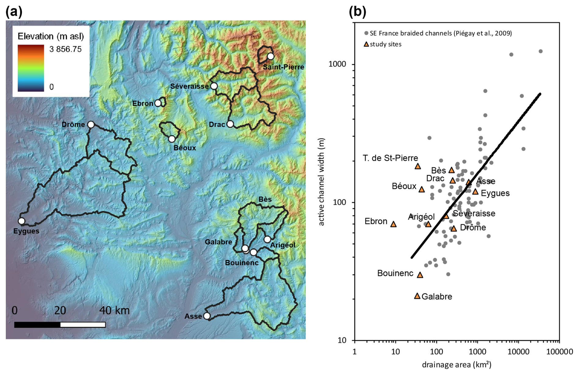
Figure 1 (a) General map of the study sites, with catchment divides in black; (b) ranking of the study sites with respect to the regional relationship of active channel width vs. drainage area for braided channels in SE France (from Piégay et al. 2009).

The last generation of remotely sensed grain-size mapping approaches is based on the use of uncrewed aerial vehicles (UAVs), which offer operational flexibility and a more affordable solution than all the other technologies used until now. The first application of drones for surface grain-size mapping was implemented in a 1 km reach of a gravel-bed river in Canada, where texture extracted from a 5 cm resolution ortho-image was used for grain-size extraction on exposed gravel bars using a local calibration curve (Tamminga et al., 2015). Hyperscale images obtained from drones can also be used to produce dense 3D point clouds from structure from motion (SfM) photogrammetry (James and Robson, 2012; Westoby et al., 2012), from which surface roughness can be used to map grain size, following the approach developed with laser scanning datasets. The first reported field experiment for river sedimentology using SfM data showed that a local calibration curve for exposed areas of a braided channel reach can be obtained with SfM point clouds, with a point density (40–900 points m⁻²) much lower than that obtained with laser scanning (Vázquez-Tarrío et al., 2017). Similar results were obtained earlier with an SfM dataset covering a moraine complex (Westoby et al., 2015). Another experiment in a small stream dominated by cobbles and boulders revealed that 3D topographic data derived from drone images offer a better grain-size prediction than 2D textural patterns in the imagery (Woodget and Austrums 2017). However, when image quality is improved with camera-stabilizing gimbals, texture extracted from single drone images offers a better grain-size prediction than roughness (Woodget et al., 2018). Beyond the local demonstration of sedimentological applications from 3D point clouds, a strong variability in empirical relationships emerges from case studies. A series of field and laboratory SfM experiments were designed to explore controlling factors for this variability and provide insights on the effects of sediment sorting, particle shape, and grain packing in the roughness calibration curve (Pearson et al., 2017). Comparison of roughness metrics derived from 3D point clouds obtained from SfM and TLS surveys of the same gravel bar showed that differences obtained between surveying methods are much smaller than those related to the grid resolution used for surface detrending (Neverman et al., 2019). This illustrates that differences in roughness calibration curves are not only related to local sedimentological properties but also to data processing protocols.

The most recent innovations in drone applications for grain-size mapping are related to direct georeferencing and to data processing using data-driven machine learning. The robotic photosieving approach based on a low-cost multirotor drone equipped for direct georeferencing allowed the production of undistorted near-ground images scaled with an SfM workflow and then processed with the photosieving program BASEGRAIN (Detert and Weitbrecht, 2012) to automatically obtain a grain-size distribution (Carbonneau et al., 2018). Field testing of this approach demonstrated that robotic photosieving GSDs are statistically equivalent to those obtained with a traditional SfM workflow, confirming that high-quality grain-size data can be directly obtained from drones without the need of ground control points (GCPs). However, robotic photosieving implies the acquisition of close-range drone images (< 10 m from the ground), and its application domain is spatially limited to short river reaches or small, dry exposed areas of river channels. Another recent advance in SfM sedimentology is the data-driven approach for extracting GSD from drone images recently tested on 25 gravel bars along six rivers in Switzerland (Lang et al., 2021). A convolutional neural network model calibrated with a training dataset extracted from close-range drone images (10 m flight height, 0.25 cm resolution) was successfully used to extract the full GSD and characteristic mean diameters of sediment on gravel bars. Although the good performance of this approach is conserved up to image resolutions around 1–2 cm, the quality of grain-size mapping products with such an approach remains to be tested with high-elevation drone surveys more suitable for covering kilometer-scale river reaches. A data-driven approach for grain-size mapping in river channels can also be applied to airborne lidar data, as recently demonstrated in a 37 km reach of a gravel-bed river (Díaz Gómez et al., 2022).

This paper explores the grain-size patchiness of 12 braided gravel-bed rivers of SE France using SfM 3D point clouds derived from high-resolution imagery obtained from a drone equipped for RTK direct georeferencing. This technological innovation is expected to improve the quality of SfM 3D point clouds while saving time in the field by reducing the need for ground control points (Hugenholtz et al., 2016; Grayson et al., 2018; Chudley et al., 2019; Stott et al., 2020), but it has rarely been tested for sedimentological applications. The only reported field testing is based on close-range UAV surveys at the gravel bar scale (Mair et al., 2022), but more investigations are needed to evaluate reach-scale applications of this approach. Specific objectives are (1) to evaluate the overall performance of the reach-scale surface grain-size prediction derived from SfM grain-scale topography obtained with RTK direct georeferencing, (2) to evaluate the transferability of the grain-size prediction for braided fluvial environments, and (3) to explore applications of the method for mapping and characterizing the grain-size patchiness of braided rivers.

Table 1 Main physical features of the 12 study sites.

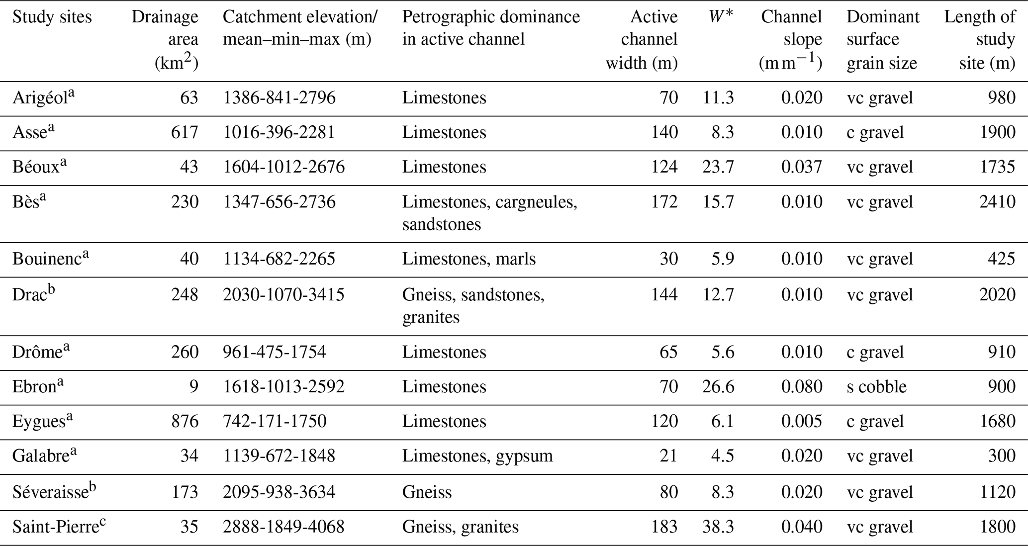
W^∗: normalized active channel width; ^a: Mediterranean flow regimes; ^b: snowmelt flow regimes; ^c: nivo-glacial flow regime. The dominant surface grain size of each study site is based on the visual inspection of high-resolution ortho-images produced for this study (s: small; c: coarse; vc: very coarse); names of grain-size classes correspond to the Wentworth scale.

2 Methodology

2.1 Study sites

The study sites are composed of 12 well-preserved braided river reaches located in the Southern French Alps and Prealps (Fig. 1a; Table 1). Spatial extents (kml file) of the 12 study reaches are available in the Supplement. Drainage areas vary from 9 to 876 km², and active channel widths vary from ∼ 20 to ∼ 200 m. The selected reaches exhibit typical morphological and sedimentological features of alpine braided channels, with multiple low-flow channels separating unvegetated gravel bars of varying size, shape, and surface texture (Fig. 2). Active channels are composed predominantly of gravels and cobbles, with local patches of fine-sediment deposition (sands and silts) (Fig. 2c). Local concentrations of small boulders are also present on proximal sites (drainage areas less than ∼ 100 km²; Fig. 2d). Most of the study sites are located in the subalpine sedimentary domain, with limestone rocks constituting the dominant lithology of the bed material. Only two sites are draining the crystalline domain of the inner Alps, in the Ecrins Massif (Séveraisse, Torrent de Saint-Pierre). The bed material is dominated here by granite and gneiss rocks. The Drac is a hybrid site characterized by more contrasted lithological conditions, with ca. 80 % of the catchment in sedimentary rocks (mostly sandstones) and ca. 20 % in the crystalline domain (mostly gneiss, granite, and migmatite).

The 12 study sites have been chosen to cover two gradients influencing the grain-size patchiness of braided channels. The first is the catchment-size gradient controlling the downstream fining of river channels through size-selective transport and abrasion processes. The second gradient is related to the sediment regime, from transport-limited to supply-limited regimes, which can be roughly assessed with the normalized active channel width, computed as $W^{\ast }=W/A_{\mathrm{d}}^{\mathrm{0.44}}$, where W is the active channel width (in m) and A_d is the drainage area (in km²). A regional analysis of braiding conditions in SE France has shown that these metrics can be regarded as a good proxy of the sediment regime of braided rivers, with increased normalized width towards transport-limited regimes (Piégay et al., 2009; Liébault et al., 2013). The study sites can be ranked according to their residual from the regional scaling law, with positive residuals for transport-limited regimes and negative residuals for supply-limited regimes (Fig. 1b). A coarser GSD is expected for threads (low-flow channels) of supply-limited regimes, as compared to transport-limited ones, under vertical size sorting effects.

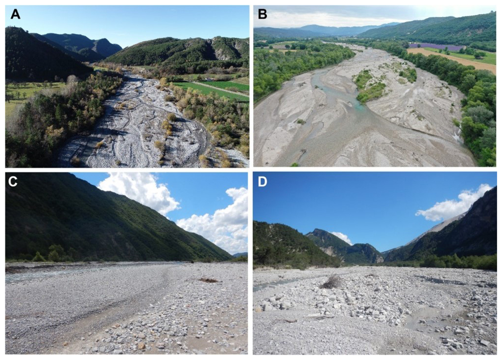
Figure 2 Pictures illustrating typical morphological and textural patterns of the study sites: aerial (drone) views of the Arigéol (a) and Asse (b) braided channels; surface grain-size patchiness of the Bès (c) and Béoux (d) braided channels; views looking upstream.

A survey reach was selected for each site, with a length approximately equal to 15 times the mean active channel width. The locations of these reaches were chosen to avoid local morphological effects related to common human pressures, such as embankments, as much as possible. The main reason is related to an objective of comparing morphological signatures of undisturbed braided channels, which is not addressed in the present paper. Field surveys took place during low-flow conditions: in autumn for snowmelt and glacial-melt rivers and in late spring and summer for Mediterranean rivers.

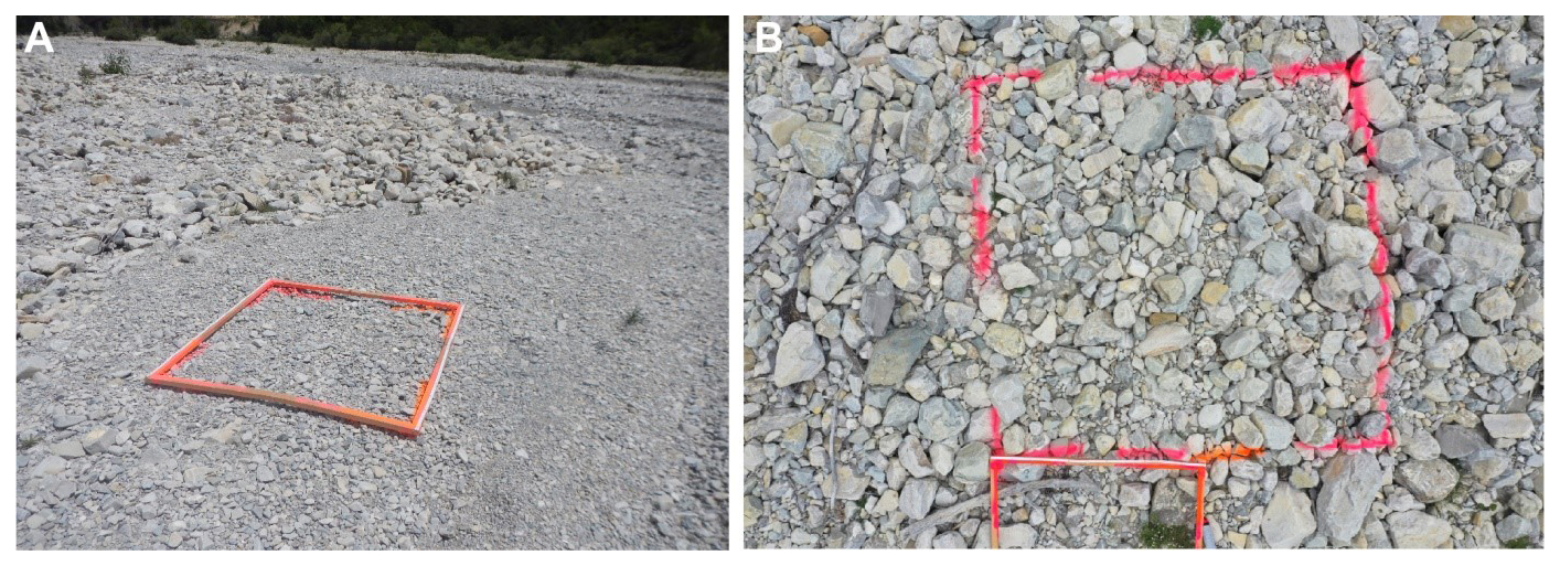
Figure 3 Examples of sampling plots used for the field calibration of grain-size proxy derived from 3D point clouds: (a) 1 m² plot used for sampling a patch dominated by gravels, Béoux site; (b) 4 m² plot used for sampling a patch dominated by cobbles and small boulders, Béoux site; the wooden frame used for marking the plots and the rule used for scaling images are visible in each picture.

2.2 Grain-size calibration dataset from close-range imagery

Calibration of the grain-size proxy derived from 3D point clouds was obtained from close-range photosieving using a set of images collected in the field with a drone flying at a very low relative elevation from the ground. Field sampling and data processing procedures of this calibration dataset are presented here.

2.2.1 Field sampling of surface grain size

For each of the 12 study reaches, the dominant grain-size patches of exposed (dry) areas of active channels were identified and sampled in the field by square plots of two different sizes (Fig. 3). A grain-size patch is defined here as a channel portion with a homogeneous surface GSD covering an area > 1 m². A 1 m² plot (100 cm × 100 cm) was used for patches dominated by gravels and pebbles (Fig. 3a), while a 4 m² plot (200 cm × 200 cm) was used for patches dominated by cobbles (Fig. 3b). About 10 plots were sampled per study reach, giving a total number of 129 plots. Contours of each sampling plot were marked with solvent-free spray paint in order to be detected and extracted on SfM point clouds. A wooden frame was used for marking the plots, and a rule was placed along the side of the frame for scaling images. The surface of each plot was carefully cleaned by removing vegetation (herbaceous plants and seedlings) and small woody debris before taking pictures. Plots were systematically positioned on flat and homogeneous surfaces to avoid artifacts related to local relief and poorly sorted sediment mixtures.

Plots were photographed individually by a DJI Mavic 2 drone at a height of 5 to 8 m from the ground. Obtained images have a spatial resolution comprising between 0.22 and 2 mm. Grain sizes smaller than the spatial resolution are not visible from imagery, and GSDs obtained from close-range photosieving must be regarded as truncated at their lower tail, at ∼ 2 mm, which corresponds to the upper size limit of very coarse sands.

Table 2 Resolution and point density of photogrammetric outputs from Agisoft Metashape.

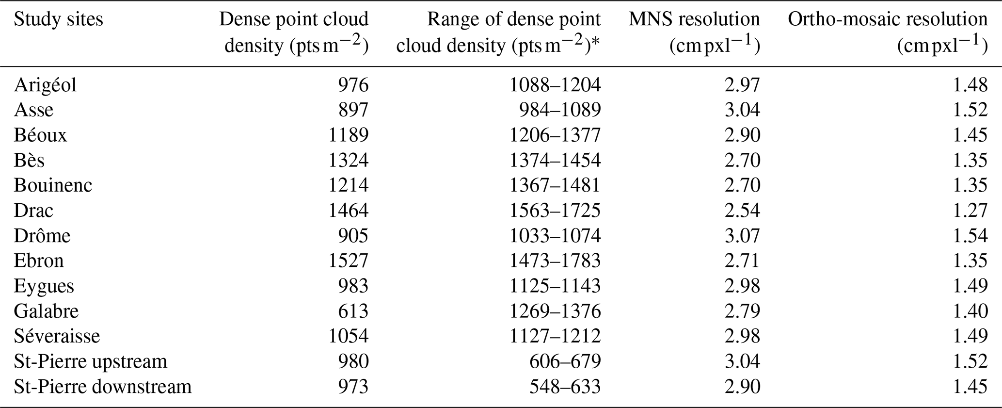
^∗ The range of values corresponds to the 25th and 75th quantiles.

2.2.2 Photosieving with Digital Grain Size

Close-range images were processed with the Digital Grain Size (DGS) code developed by Buscombe (2013), which automatically provides an estimate of the statistical GSD from an image. The apparent GSD in the image is estimated by deriving the global spectral density power function using Morlet wavelets. The use of Morlet wavelets allows the simultaneous quantification of spatial and spectral information by decomposing the image into variance versus frequency. This method has the advantage of being fast and free of a calibration phase, which theoretically gives it a universal scope. DGS processing of images provides the grid-by-number frequency of grains as a function of their diameter and the GSD percentiles. A normalized root-mean-square error ($\text{nRMSE}=\text{RMSE}/D_x$, with D_x the percentile of rank x) for the D₅₀ typically less than 20 % can be achieved when the sample size is at least 250 grains per image (Buscombe, 2013). This code was chosen instead of the more recent machine learning SediNet code developed by the same author (Buscombe, 2020) on the basis of results reported by Chardon et al. (2022), showing a better performance with DGS for a set of digital images of gravel bars collected on the Rhine River.

Following recommendations of Chardon et al. (2020), who tested the performance of DGS photosieving on exposed gravel bars of the Rhine River, images were corrected using a median filter with a radius of 5 % of the largest particle sizes. This correction attenuates errors related to intra-grain petrographic variations and allows a reduction of the D₅₀ nRMSE from 72 % to 29 %. This improvement was confirmed by our dataset, and only data from filtered images are presented here. The study by Chardon et al. (2020) also showed that solar lighting conditions and sampling area have an effect on DGS performance. It was therefore necessary to produce a calibration dataset for controlling and calibrating DGS-derived GSDs.

2.2.3 Calibration of DGS grain-size percentiles with ImageJ

A total of 44 plots were sampled for testing the quality of GSDs obtained from DGS (10 from the Galabre, 11 from the Arigéol, 3 from the Torrent de Saint-Pierre, 9 from the Ebron, and 11 from the Eygues). The open-source image processing software ImageJ (https://imagej.net/ij/, last access: 17 July 2025) was used for the manual extraction of apparent diameters visible on the selected images. This software allows the positioning of a grid on the images, the manual segmentation of the grains, and the extraction of b axes, following a commonly used protocol of on-screen manual extraction of apparent diameters of grains (Graham et al., 2005b; Barnard et al., 2007; Buscombe, 2013; Chardon et al., 2022). At least 100 grains were measured on each image. Distances between grid nodes were fixed at 10 cm for 1 m² plots and 20 cm for 4 m² plots for maximizing the number of grains while avoiding sampling the same grain twice. These manual grain-size measurements were used to verify and calibrate the automatic results produced by DGS. GSDs from ImageJ were regarded as pseudo-ground-truth data, since only apparent diameters can be extracted from images, which are different from true diameters that can be directly measured in the field using a classic pebble count. This is known as the fabric error, which is related to individual grain inclination and partial hiding (Graham et al., 2005a). However, several studies based on field measurements of the b axis using the paint-and-pick approach demonstrated that this systematic error is low for grid-by-number sampling, typically comprising between 0.05 and 0.45 ψ (ψ = log₂D, where D is the grain diameter in mm) (Graham et al., 2005a; Dugdale et al., 2010). Since sediment patches from our study reaches are composed of loose grains without strong imbrication and packing, we assumed that the systematic bias from true percentiles is low (likely less than 0.45 ψ).

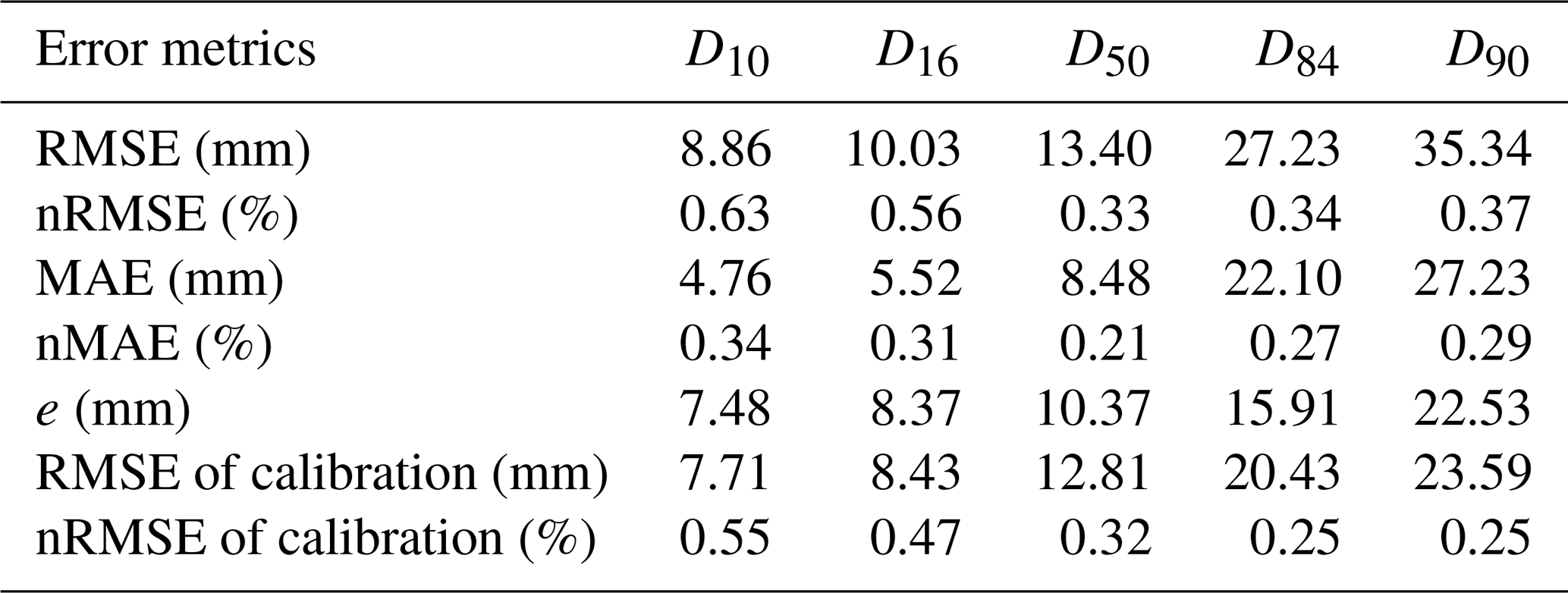
The calibration of DGS grain-size percentiles was obtained by regression analysis with manually extracted percentiles from ImageJ. The root-mean-square error (RMSE), the mean absolute error (MAE), and the irreducible random error (e) of DGS percentiles (for both raw and calibrated values) were calculated, respectively, as

$$\begin{array}{}\text{(1)}& {\displaystyle }& {\displaystyle }\text{RMSE}=\sqrt{{\displaystyle \frac{{\sum }_{i=\mathrm{1}}^n(D_{\text{xpi}}-D_{\text{xoi}}{)}^{\mathrm{2}}}{n}}},\text{(2)}& {\displaystyle }& {\displaystyle }\text{MAE}={\displaystyle \frac{\mathrm{1}}{n}}\sum _{i=\mathrm{1}}^n\mathrm{|}{D}_{\text{xpi}}-D_{\text{xoi}}\mathrm{|},\text{(3)}& {\displaystyle }& {\displaystyle }e=\sqrt{{\text{RMSE}}^{\mathrm{2}}-{\text{MAE}}^{\mathrm{2}}},\end{array}$$

where D_xpi is the DGS percentile of rank x, D_xoi is the manually extracted ImageJ percentile of rank x, and n is the number of plots used for calibration. The normalized RMSE and MAE were also computed to aid comparisons with previous studies (e.g., Chardon et al., 2020).

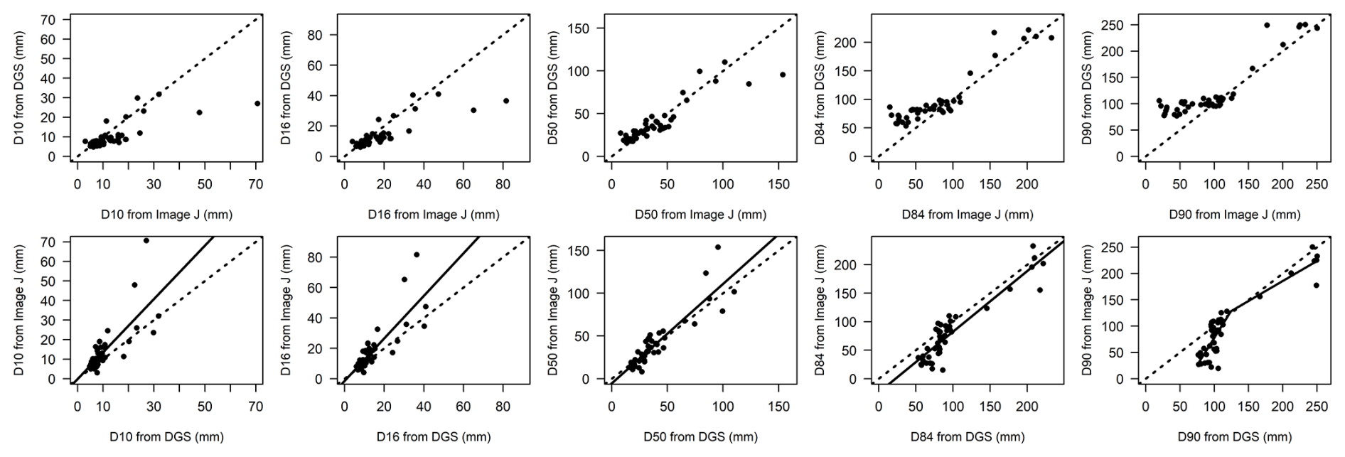
Figure 4 Comparison of grain-size percentiles computed with DGS and extracted with ImageJ; plots on the top show predicted vs. observed percentiles; plots on the bottom show the calibration curves of the DGS percentiles (full line). Dotted lines correspond to equality lines (x=y).

2.3 Grain-size proxy from 3D SfM point clouds

2.3.1 UAV surveys

UAV images were taken with a DJI Phantom4 RTK. This drone benefits from direct georeferencing. It is connected to a D-RTK mobile station, allowing drone positioning with an announced accuracy of 1 cm in x and y and 1.5 cm in z (1 mm error increase by kilometer of distance to the base). The onboard camera resolution is 20 Mpxl, with a focal length of 8 mm. The flight height was fixed at 70 m, allowing a spatial resolution of 2–3 cm on images. Images were taken during low-flow period at nadir with side and forward overlaps of 60 % and 80 %, respectively. They were also taken in the late morning and early afternoon, to avoid shadowing effects on point cloud reconstructions as much as possible. Parameters of the drone flights were programmed with the DJI Ground Station RTK application.

Ground control points (GCPs) were marked homogeneously in each study reach with solvent-free spray paint. They were positioned along cross-sections spaced at a regular interval equal to the mean active channel width. Their coordinates were measured either with a Leica Zeno 20 dGPS or with a GPS Leica GS20 and a rover Leica GS10. The Leica Zeno 20 provides corrected GNSS RTK positions and benefits from the coverage of the GPS, Glonass, and Galileo networks. The measurement accuracy announced by the manufacturer is less than 5 cm + 1 ppm in horizontal and less than 2 cm + 1 ppm in vertical. The GPS Leica GS10 provides a position with an RMSE of 8 mm + 1 ppm in x and y and 15 mm + 1 ppm in z in cinematic mode and an RMSE of 3 mm + 0.5 ppm in x and y and 5 mm + 0.5 ppm in z in static mode.

Table 3 Error metrics of DGS percentiles obtained on close-range grain images after application of a median filter; the root-mean-square errors of calibration curves obtained for the different percentiles are also indicated (see Sect. 2.2.3 for definitions of the metrics).

2.3.2 SfM photogrammetry and roughness extraction

An SfM photogrammetric processing of UAV images was performed using the Agisoft Metashape software (version 1.7.3) to produce a dense point cloud, a digital surface model (DSM), and an ortho-image. The SfM workflow was built following recommendations available in the literature (Eltner et al., 2016; James et al., 2020; Over et al. 2021) to get the best outputs regarding the performance of the computer. The sparse point clouds were obtained by the alignment of the photos using a high accuracy. Poor-quality points were removed, ground control points were imported, and cameras were optimized several times. The dense points clouds construction was done by setting high quality and mild depth filtering. The workflow is presented in detail in the Supplement, with different metrics of error.

Metric errors (mean error, mean absolute error, and standard deviation of error) of the camera location for the z coordinate are automatically calculated by Agisoft Metashape during the reconstruction of the 3D model (Alignment tool) and the densification of the cloud. Results show a good accuracy of the dense point clouds with a standard deviation of error for the z coordinate of the camera ranging from 0.98 cm (Galabre) to 4.6 cm (Drac). Errors computed with control points (dGPS markers used to georeference the 3D model) and check points (dGPS markers not used to optimize the camera alignment) are also provided in Table S1 in the Supplement. RMSE values of elevations computed on check points are generally less than 10 cm, except for four sites (Asse, Drac, Drôme, and Ebron). The mean point density of all the dense point clouds is 973 points m⁻², and the resolution of ortho-mosaic ranges from 1.27 to 1.54 cm (Table 2).

SfM point clouds were imported in CloudCompare (version 2.12.0) (https://www.danielgm.net/cc/, last access: 17 July 2025) to manually segment the sampling plots at each study reach and compute their roughness height. This metric is defined as the shortest distance between a given point and the best-fitting plane calculated on its nearest neighbors included in a sphere of predetermined radius (CloudCompare, 2021). It is now regularly used as a grain-size proxy (Vázquez-Tarrío et al., 2017; Woodget and Austrums, 2017; Chardon et al., 2020). The radius for calculating roughness height was determined from a sensitivity analysis allowing us to choose an optimum value. An initial value of 0.1 m was chosen and incremented by 0.1 m up to a maximum value of 1 m. The radius showing the best correlation between roughness height and D₅₀ was chosen as the optimal value (Fig. S1 in the Supplement). Percentiles of the roughness height distributions were used as predictors of corresponding grain-size percentiles (D₁₆, D₅₀, and D₈₄). The mean roughness height was also used as a predictor for the D₅₀. All these predictors were compared to corrected grain-size percentiles derived from close-range photosieving, through regression analysis.

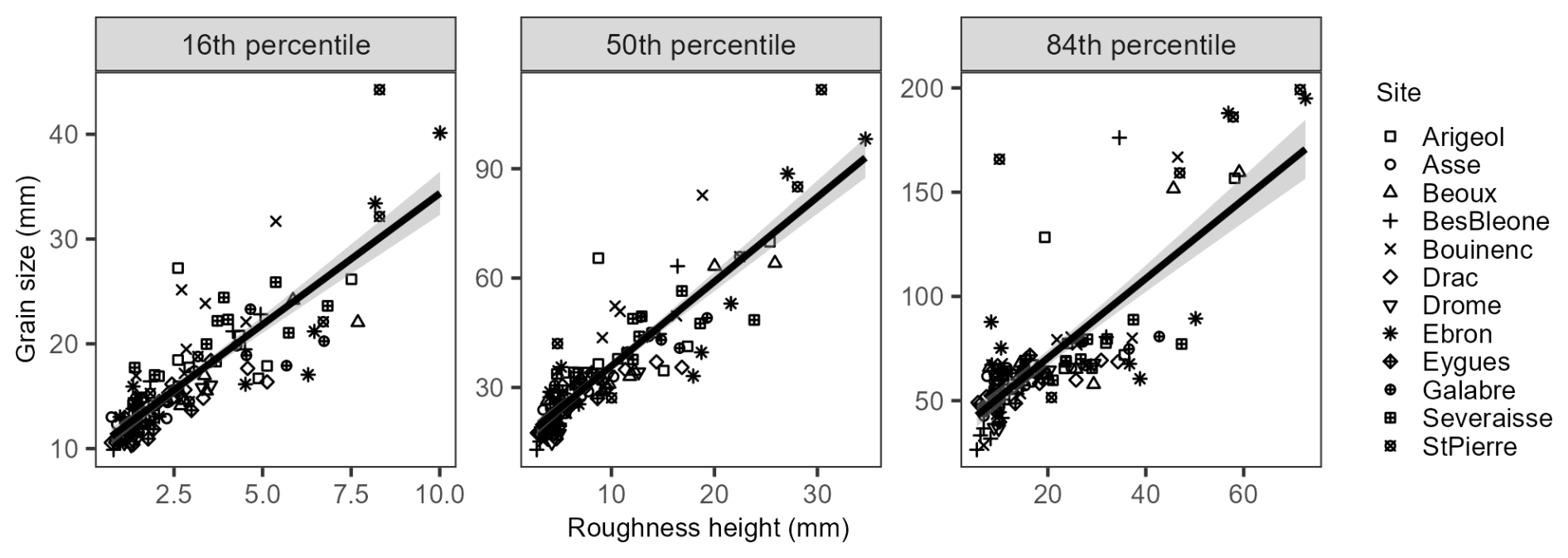
Figure 5 Calibration curves of grain-size percentiles based on corresponding roughness height percentiles. Shaded areas correspond to the 95 % confidence interval of the regressions.

Figure 6 Calibration curves of grain-size percentiles based on the mean roughness height. Shaded areas correspond to the 95 % confidence interval of the regressions.

2.3.3 Jackknife cross-validation of the grain-size proxy

Validation of grain-size calibration curves was done using a leave-one-out cross-validation (LOOCV) jackknife procedure (Quenouille, 1956; Woodget and Austrums, 2017). This iterative procedure was used to compute linear regression fits using 128 of the 129 sampling plots and to predict grain size of the excluded plot. This procedure was reiterated 129 times to independently assess the accuracy and precision of each calibration curve. Another jackknife procedure was used to assess the transferability of the calibration curves to study reaches that have not been used for calibration. It was performed by excluding all the plots from one given study reach. The grain size of that study reach was then predicted with the calibration curve obtained from the other study reaches to evaluate the transferability. This procedure was reiterated 12 times so that the error of transferability was computed for each study reach.

2.3.4 Active channel grain-size maps

The D₅₀ calibration curve was used to produce a distributed grain-size map of active channels (dry and wet surfaces) for each study site. After creating a mask of the active channel including unvegetated gravel bars and low-flow channels, non-alluvial elements (large woody debris, artificial objects) were manually removed. Small vegetated patches included in the active channel were filtered with the automatic classification tool available in Agisoft Metashape (Classify ground points tool). An in-house R script based on the Excessive Greenness index (ExG) (Woebbecke et al., 1995; Núñez-Andrés et al., 2021) was written to remove unfiltered vegetated patches from Metashape. Steep surfaces of the active channel (e.g., bar talus) were also excluded, since they are characterized by high roughness values not related to grain size but to the local relief. A slope threshold of 60 % was used to remove these steep surfaces, except for the Asse, where it was necessary to use a threshold of 30 % to exclude bar talus. No slope threshold was used for the Ebron because its active channel presents a coarse surficial grain size without any clear effect of local slope on roughness heights.

Filtered dense point clouds were imported in CloudCompare to compute the roughness height using the optimal radius obtained from the sensitivity analysis (see Sect. 2.3.2). A 1 m resolution raster of roughness was produced by averaging roughness values for each pixel. Finally, the calibration curve was applied on every pixel to get the corresponding D₅₀. Each pixel was then included in a grain-size class using the Wentworth scale (Wentworth, 1922) and considering half-phi and phi size limits for gravels and cobbles, respectively. Relative proportions of grain-size classes were then compared between study reaches, with respect to drainage areas.

A specific field sampling was undertaken to determine if grain-size maps can provide accurate reach-scale estimates of the mean surface D₅₀ of the active channel and of different geomorphic units of the active channel (unvegetated bars and low-flow channels). This was done for the Arigéol and the Drac, from Wolman pebble counts along 10 cross-sections spanning the whole active channel, established at 100 m (for Arigéol) and 250 m (for the Drac) spacing, with a sampling interval of 1 and 2 m for the Arigéol and the Drac, respectively (cross-section maps are provided in Figs. S2 and S4 in the Supplement). This corresponds to the spatially integrated sampling scheme for determining a reach-averaged GSD (Bunte and Abt, 2001). Sampling points located in bars and low-flow channels were informed during the field sampling, in order to compute composite GSDs of these two geomorphic units. The assemblage of all sampling points was used to compute the active channel GSD. A similar field sampling was initially planned for a third site (Bouinenc), but, for logistical reasons, Wolman pebble counts were restricted to a single point bar where particles were collected at 1 m intervals along two longitudinal sampling lines (Fig. S3). Confidence intervals (95 %) of the D₅₀ obtained from composite distributions were computed using the GSDtools package developed by Eaton et al. (2019).

Table 4 Linear regressions of grain-size percentile calibration curves with their jackknife residual errors.

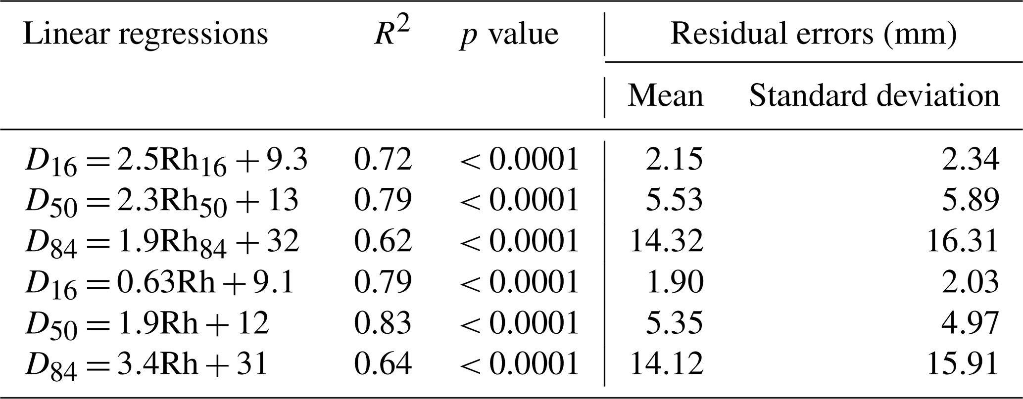
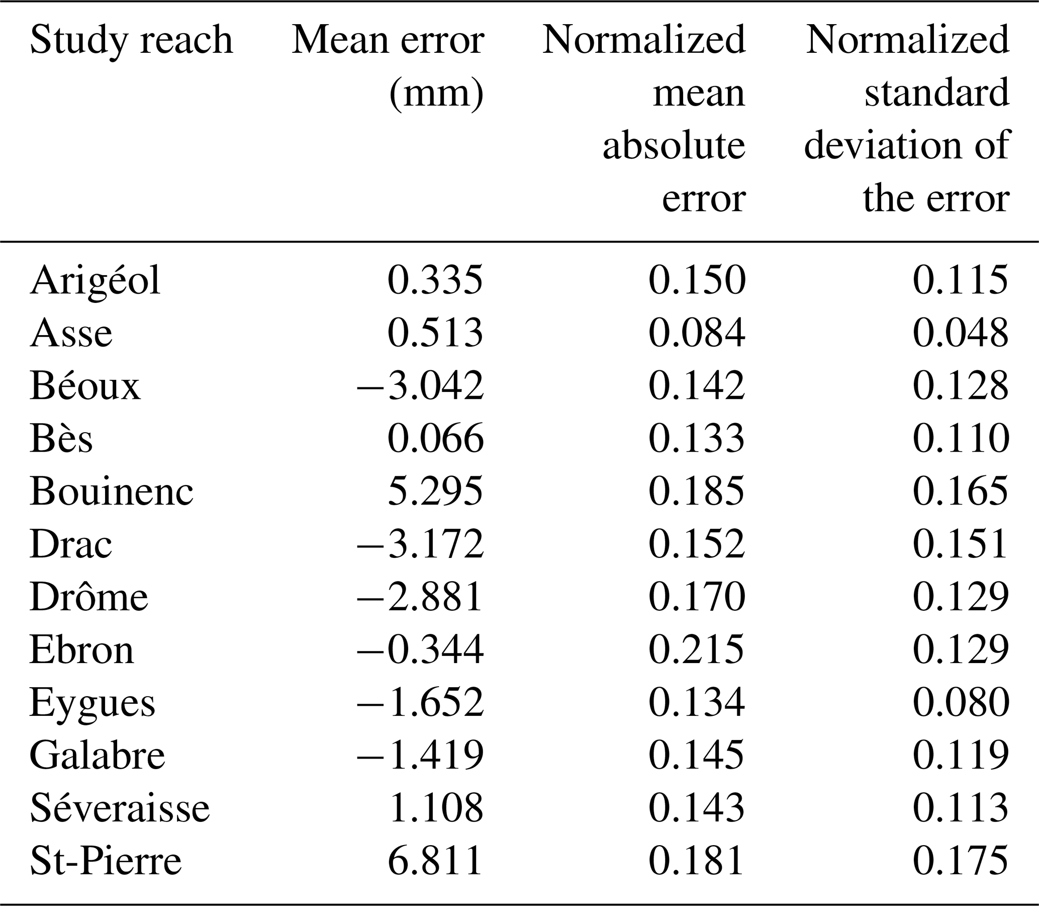
Table 5 Metrics of error of the D₅₀ obtained from the jackknife resampling procedure based on site exclusion (transferability analysis).

Field samples were collected in early 2024 and were compared with grain-size maps extracted from UAV images taken in November 2020 (Arigéol and Bouinenc) and March 2024 (Drac). No major morphological changes occurred between 2020 and 2024 along the Arigéol study reach, and it is assumed that the reach-scale-averaged surface GSDs remained unchanged during this period. The investigated point bar of the Bouinenc also remained unchanged during this period. This is not the case of the Drac study reach, which has been modified by an active hydrological period that occurred in October 2023 (peak discharge with a 10-year return period). Therefore, field-based GSDs were compared to a grain-size map extracted from UAV images taken the same day as the field survey (March 2024). A comparison was also made with a grain-size map extracted from images of September 2021.

The extraction of reach-averaged D₅₀ of unvegetated bars and low-flow channels from grain-size maps was done from a manual digitizing of bars using SfM DEMs and ortho-images (see Fig. S5 in the Supplement for an example). Two procedures were used to select bar pixels for grain-size extraction. The first one considers all the pixels totally included in bar polygons. The second one is based on a selection of bar pixels regarded as valid. A 4 m² sampling grid (i.e., 4 grain-size pixels) was superimposed on the ortho-image to carry out a selection based on a qualitative inspection of the bar surface. Only grid cells with at least 90 % of the surface composed of clean, coarse (gravel, cobble) alluvial sediment were considered valid. This allows us to exclude bar pixels where surface roughness is partly controlled by woody debris or fine-sediment deposits (silts) and thus to include only those pixels that are similar to the sampling plots used to calibrate the roughness proxy. The low-flow channel D₅₀ was extracted from pixels that are not included in digitized bars. Finally, the active-channel D₅₀ was obtained by averaging bar and low-flow channel pixels.

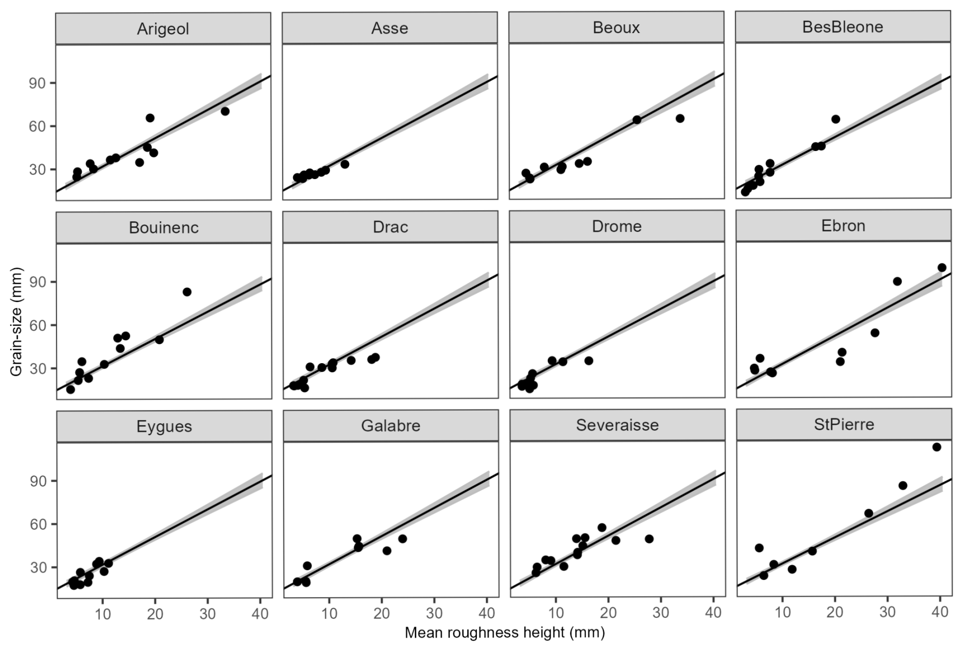
Figure 7 Assessment of the transferability of the D₅₀ calibration curve. For each plot, linear regressions were obtained after the exclusion of calibration plots from the mentioned study reach. Points represent calibration plots of the excluded study reach. The shaded area represents the 95 % confidence interval of the regression.

3 Results

3.1 Photosieving with DGS

Grain-size percentiles obtained from close-range automatic photosieving with DGS were compared with those obtained from manual extraction of apparent particle diameters with ImageJ (Fig. 4). DGS performance was thus tested for a wide range of grain sizes (8 mm < D₅₀ < 154 mm), representative of the sedimentological variability in study reaches. A systematic underestimation of low percentiles (D₁₀ and D₁₆) was observed, while high percentiles (D₈₄ and D₉₀) were consistently overestimated. Medians of the computed distributions are closer to the equality line, except for two points with a manually extracted D₅₀ above 120 mm for which a strong (∼ 35 %) underestimation was observed.

The DGS performance for D₅₀ prediction is not as good as expected, with an nRMSE of 33 %, an nMAE of 21 %, and an irreducible error of 10.37 mm (or 3.37 ψ) (Table 3). The best performance was obtained for the D₅₀ and the D₈₄. If the two outliers with a manually extracted D₅₀ above 120 mm are excluded, nRMSE and nMAE for the D₅₀ fall at 24 % and 18 %, respectively. Those outliers correspond to two large sampling plots established on well-sorted cobble bars of the Ebron site. Although the number of grains on those two images is low, it stays close to the recommended limit of 250 grains per image, below which DGS performance strongly drops. If the ratio between the grid sampling interval and the b axis of the largest grain is considered, those two outliers do not show particularly low values that could explain a strong bias of DGS or ImageJ values of their median grain sizes. Their ratio values (0.52 and 0.74) are lower than the average value (0.96), but many calibration plots present lower values, and it is not possible to justify their exclusion from the calibration curve using this criterion.

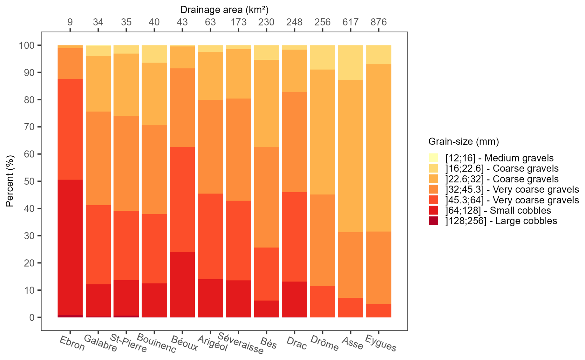
Figure 8 Grain-size distributions of the active channel for each study reach arranged in order of increasing drainage area.

Linear regressions offer the best fits for the D₁₀, D₁₆, D₅₀, and D₈₄ calibration curves (Fig. 4). However, normalized errors of calibration stay above 45 % for the lower percentiles, and a value of 32 % is obtained for the D₅₀. The best calibration curve for the D₉₀ was obtained using a piecewise regression function allowing the automatic detection of breakpoints in the regression line (Muggeo, 2008). This regression model is justified by an evident break of slope visible on the scatterplot of the highest percentile, revealing that a linear model is not really appropriate for this dataset. A piecewise function was also tested for the D₈₄ but without any success because the change in slope above the suspected breakpoint is too low (points with ImageJ-derived D₈₄ above 120 mm). The best calibration curves are those obtained for high percentiles, with nRMSE around 25 %.

3.2 Grain size from SfM 3D point clouds

3.2.1 Calibration curves based on roughness height

The optimum radius for calculating roughness height determined from the sensitivity analysis comprises between 0.4 and 0.5 m (Fig. S1). A value of 0.5 m was chosen for the computation of roughness predictors. This value is the same as that obtained by Vázquez-Tarrío et al. (2017) in a braided channel, and it represents approximately twice the largest grain observed in the dataset. Calibration curves obtained for grain-size percentiles (D₁₆, D₅₀, D₈₄) using corresponding roughness height percentiles (Rh₁₆, Rh₅₀, and Rh₈₄) and the mean roughness height (Rh) are presented in Figs. 5 and 6, respectively. Regression equations and parameters are displayed in Table 4 along with metric errors computed by the jackknife method. Linear regressions systematically offer the best fits for every tested proxy, and the best calibration curve was obtained for the D₅₀ as a function of the mean roughness height (R² = 0.83). This calibration curve shows an independent error of prediction of 4.97 mm, which corresponds to 14.4 % of the mean D₅₀ computed for the 129 calibration plots (34.47 mm). Generally speaking, and whatever the considered grain-size percentile, better results are obtained with the mean roughness height, compared to roughness percentiles. Better results are also obtained for D₁₆, compared to D₈₄. The high data scatter observed for the D₈₄ diagram shows that the roughness height is not a good proxy of the coarse surficial grain size.

3.2.2 Transferability of the D₅₀ calibration curve

To test the transferability of the D₅₀ calibration curve to other braided rivers, a jackknife resampling was undertaken to evaluate expected deviations from the curve once applied to a study reach not included in the calibration. Results are shown in Fig. 7. For each diagram, the calibration curve was established after excluding all the plots from one given study reach. Points in each diagram correspond to the plots of the excluded study reach. The mean error, the normalized mean error, and the normalized standard deviation of error specific to each study reach were calculated in order to quantify accuracy and precision (Table 5). The normalization was made using the mean D₅₀ of each study reach. The standard error of the prediction residual varies from 5 % to 17.5 % (Asse and St-Pierre, respectively). This result is in good agreement with the independent prediction error of the D₅₀ calibration curve. Asse is the site for which points are closer to the calibration curve, with the lowest normalized mean error. However, calibration curves tend to overestimate the median grain size of Béoux, Drac, and Drôme and underestimate those of Bouinenc and St-Pierre.

3.3 Surface grain-size mapping

3.3.1 Grain-size distributions of the 12 study reaches

The D₅₀ calibration curve (D₅₀ = 1.9Rh+12; Table 4) was used to produce distributed 1 m resolution grain-size maps of active channels for the 12 study reaches, from which composite GSDs of the active channel were extracted. These composite GSDs are arranged in ascending order of drainage area for inter-site comparison (Fig. 8). A pattern of large-scale downstream fining clearly emerges, with an increasing proportion of fine fractions (coarse gravels) with drainage areas. More specifically, most of the study reaches with drainage areas between ∼ 30 and ∼ 200 km² share very similar GSDs, with around 40 % of the active channel presenting a D₅₀ above 45 mm. One exception is the Béoux, showing a coarser GSD, likely related to high sediment supply from a very active debris-flow torrent located a few hundred meters upstream of the study reach. A regular downstream fining is observed for drainage areas above 200 km², except for the Drac, showing a GSD similar to small catchment sizes. This can be related to the geological specificity of this site, compared to other study reaches with large catchment sizes, which are all included in the sedimentary domain. This is not the case of the Drac, where an important part of its catchment is composed of very resistant crystalline rocks (gneiss, granites, and migmatites).

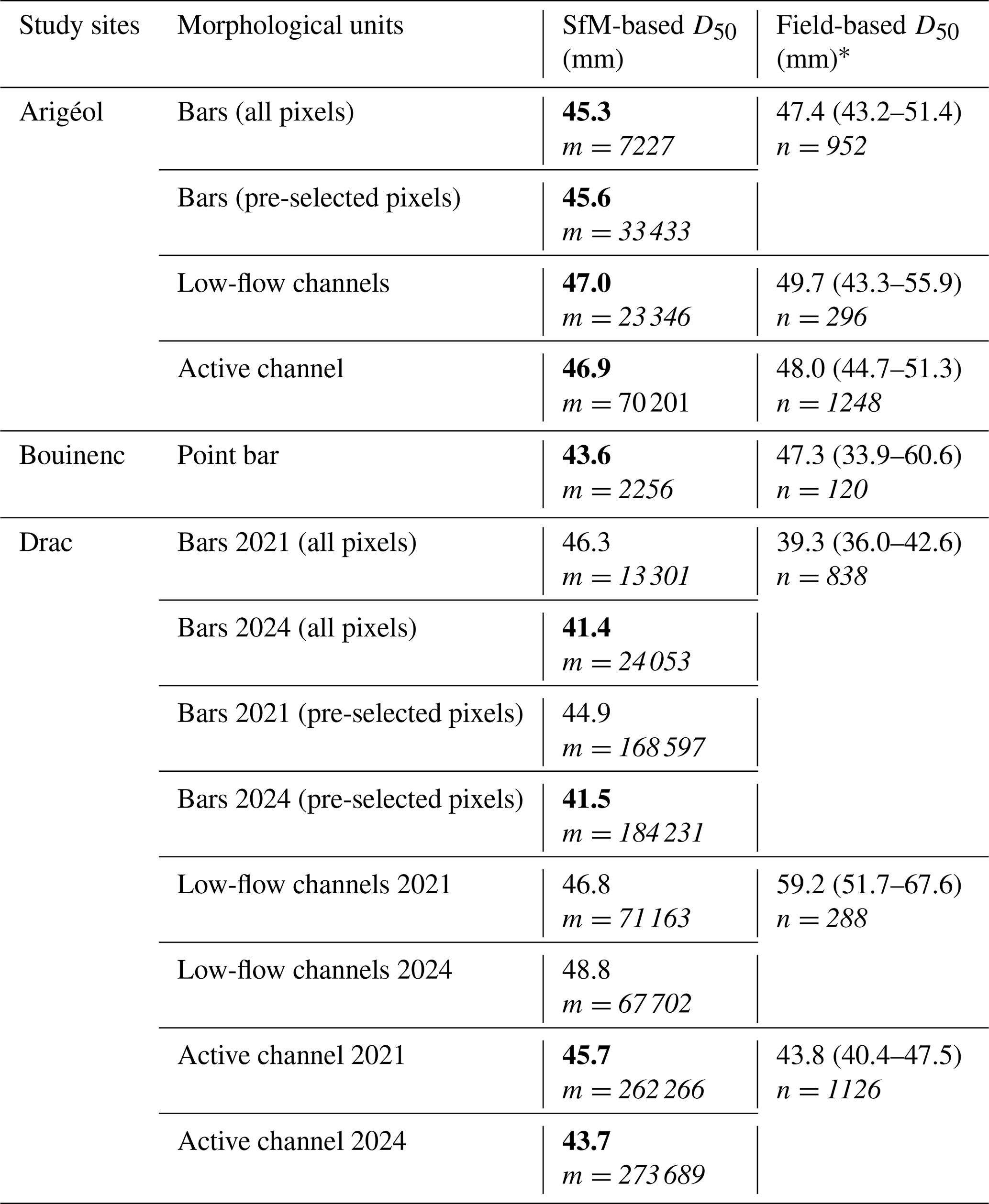
Table 6 Comparison of D₅₀ obtained by Wolman samplings (field-based) and by grain-size mapping (based on the roughness proxy computed with SfM 3D point clouds) for different geomorphic units and for the whole active channels; m is the number of pixels, and n is the number of particles sampled; ^∗ values in parentheses correspond to the 95 % confidence interval of the D₅₀ computed with GSDtools (Eaton et al., 2019); SfM-based D₅₀ values in bold are those included in the 95 % confidence interval of the field-based D₅₀; the sum of pixels in bars and low-flow channels is not equal to the number of pixels in the active channel because only pixels that are fully in each morphological unit were used.

3.3.2 Field control of SfM-based median grain sizes

The comparison of SfM-based (or roughness-based) and field-based reach-averaged D₅₀ of active channels and different geomorphic units of active channels is presented in Table 6. This comparison shows that almost all of the extracted D₅₀ values from grain-size maps are included within the 95 % confidence interval of the D₅₀ obtained by composite Wolman pebble counts. This is the case for the Arigéol, where all the SfM-based D₅₀ values can be regarded as very good estimates of “true” values observed in the field, with absolute differences always being inferior to 3 mm (less than 5 % of field-based reach-averaged D₅₀ values), including submerged portions of the active channel. A good agreement was also obtained for the investigated point bar of the Bouinenc, with an absolute difference of only 3.7 mm between field-based and SfM-based D₅₀ values (8 % of error). More contrasted results have been obtained for the Drac. Most of the D₅₀ values extracted from the 2021 imagery are not included in the 95 % confidence interval of field-based D₅₀ values. This discrepancy can be explained by an important reworking of the active channel during a series of floods that occurred in October 2023. The comparison with the 2024 imagery provides much better results, except for low-flow channels, where an underestimation of the field-based D₅₀ values is still observed (18 % of error). However, results obtained for bars and for the whole active channels confirm a very good agreement with field-based values, with absolute differences being less than 3 mm (less than 6 % of error). The pre-selection of bar pixels for exclusion of bar surfaces impacted by woody debris and fine-sediment deposits does not have a strong effect on SfM-based reach-averaged D₅₀, whether on the Drac or the Arigéol. Differences obtained between all pixels and pre-selected pixels for these two sites are extremely small (less than 1 mm) and do not justify any exclusion procedure for the computation of reach-averaged median grain size of bars.

Table 7 Statistical analysis of grain-size heterogeneity along sampled cross-sections of the Arigéol and Drac study reaches.

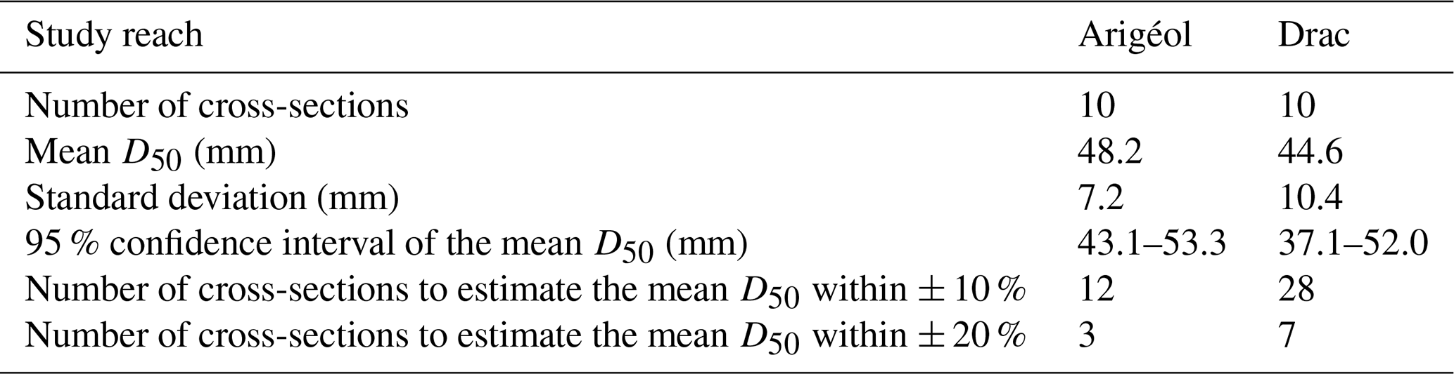
The representativity of reach-averaged D₅₀ obtained from the spatially integrated field sampling can be assessed through the analysis of grain-size heterogeneity between sampled cross-sections at a given site (Mosley and Tindale, 1985). Confidence intervals of the mean D₅₀ were computed with the t distribution at a 5 % risk of error, and the number of cross-sections (N) to estimate the mean D₅₀ at a 95 % confidence level was computed as

$$\begin{array}{}\text{(4)}& N={\left({\displaystyle \frac{t_{n-\mathrm{1}}\mathit{\sigma }}{\text{me}}}\right)}^{\mathrm{2}},\end{array}$$

where t_n−1 is the t value for an n−1 degree of freedom (with n as the number of sampled cross-sections), σ is the standard deviation, and me is the margin of error of the mean. This analysis shows a higher grain-size heterogeneity for the Drac and, subsequently, a lower spatial representativity of the mean D₅₀ computed from the 10 cross-sections (Table 7). For this study reach, 28 cross-sections would have been necessary to estimate the mean D₅₀ within a 10 % margin of error, while the equivalent figure for the Arigéol is only 12. The equivalent sampling effort for the two study reaches (10 cross-sections) corresponds to a margin of error of 10.6 % and 16.7 % for the Arigéol and the Drac, respectively.

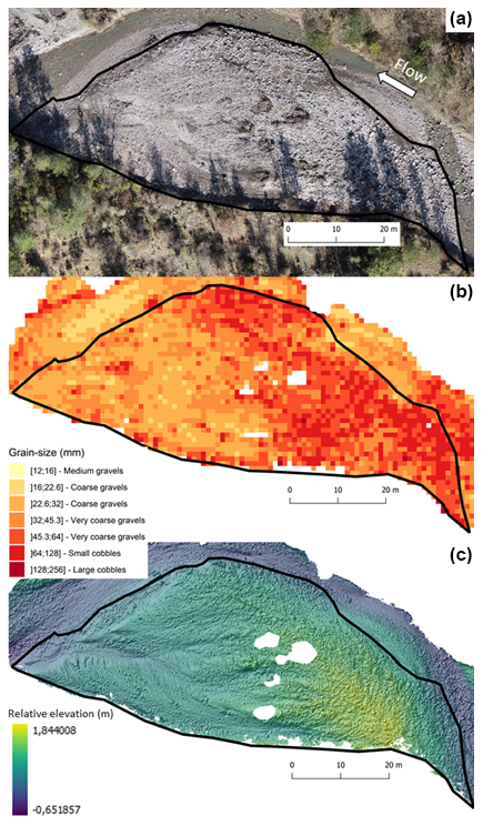
Figure 9 Morpho-sedimentary signature of a typical point bar in the Bouinenc. (a) High-resolution SfM ortho-image (1.35 cm pxl⁻¹); (b) grain-size (D₅₀) map extracted from imagery; (c) REM (2.7 cm pxl⁻¹); flow is from right to left; the black line corresponds to the point bar delimitation.

3.3.3 Bar-scale morpho-sedimentary signatures

SfM-based grain-size maps have been used to explore morpho-sedimentary signatures of bars. The morphological component of the signature has been constrained by relative elevation models (REMs), which were computed by subtracting at a 1 m interval the elevation of the active channel from the averaged elevation of the main low-flow channel (i.e., the thalweg that structured the active channel). A first example is presented at the scale of a single bar, which corresponds to the point bar of the Bouinenc that has been sampled in the field for grain-size measurement (Fig. 9). A clear sedimentological pattern typical from alternate bars is detectable here. A longitudinal grain-size gradient with a down-bar fining trend is clearly visible from the grain-size map (Fig. 9b). Coarser grain-size patches (D₅₀ > 45.3 mm) are preferentially located at the highest part of the bar, which corresponds to its head (Fig. 9b and c). This example illustrates how the classic sedimentological patterns of gravel-bed rivers can be well recognized on image-based grain-size maps.

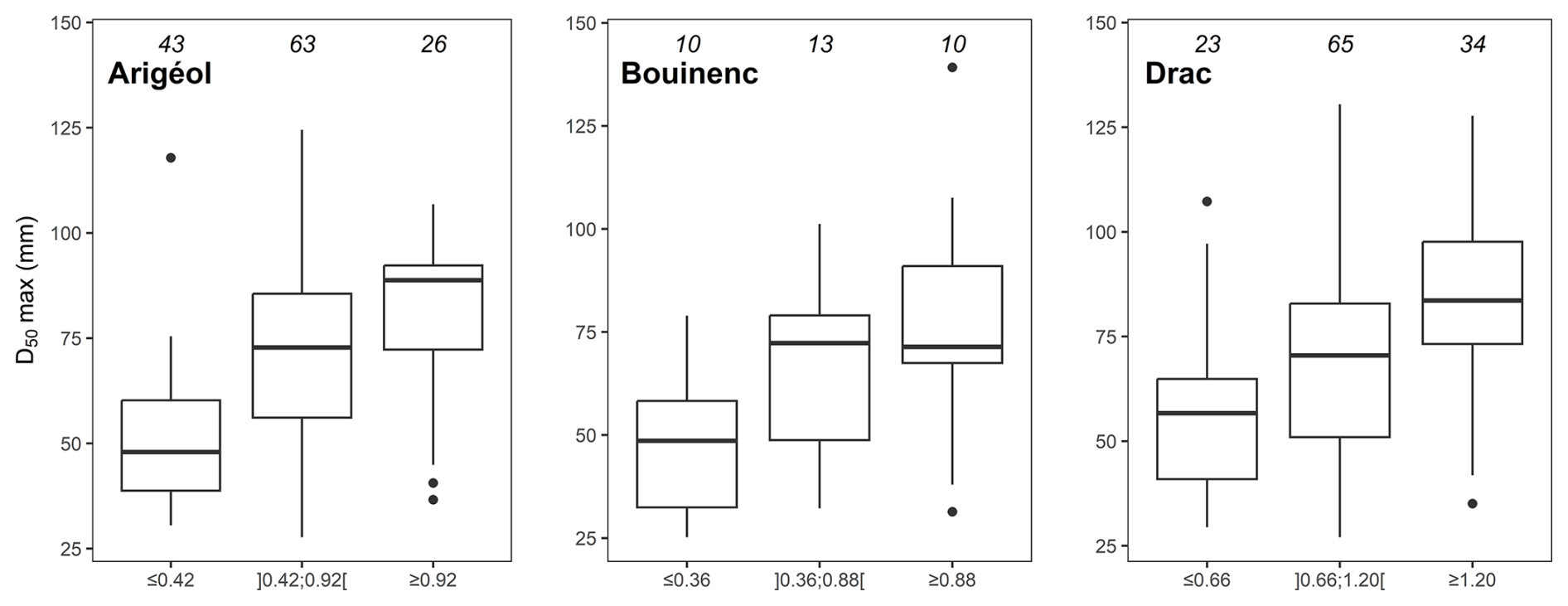
Figure 10 Maximum D₅₀ of bars as a function of relative elevation; numbers of bars for which the D₅₀ value has been extracted are indicated on tops of the box plots; quantile distributions of the relative elevation of bars for each study reach have been used for discretization (≤ Q25, ]Q25;Q75[, ≤ Q75).

A second example is provided by the exploration of the link between the surface grain size of bars and their relative elevation. This has been explored for the three study reaches where a detailed manual mapping of bars has been done (Arigéol, Bouinenc, and Drac). The distribution of the maximum D₅₀ values of bars as a function of their 90th percentile of relative elevation is presented in Fig. 10. Maximum D₅₀ values were extracted from pre-selected pixels of bars (those which can be regarded as non-affected by woody debris and/or fine-sediment deposits). Each of the study reaches shows a positive trend indicating that the relative elevation of bars has a strong effect on surface grain size. As the coarser part of bars generally corresponds to bar heads, this result demonstrates that, in many braided active channels, the coarser bar heads generally correspond to the highest bars within the active channel.

4 Discussion

4.1 Photosieving with DGS

New data have been produced to test the quality of automatic particle size extractions resulting from the processing of close-up images of gravel bars. These data are crucial for the calibration of SfM sedimentological proxies. The comparative analysis of the DGS percentiles with those obtained from the manual extraction of the apparent diameters on ImageJ shows that a field calibration of the DGS results is absolutely necessary, even for high-definition images of homogeneous sedimentary facies. A systematic bias is observed for all percentiles, with a much more pronounced shift for small percentiles. This negative bias of DGS for small percentiles was already shown by Buscombe (2013), who explains this by the high sensitivity of the wavelet approach to few numbers of the smallest grains on images. The overall performance of DGS is not as good as presented in the literature. Buscombe (2013) reported a normalized RMSE of 16 % for D₅₀ using a set of 262 unconsolidated sand/gravel images. However, DGS tests on exposed Rhine gravel bars showed a much higher normalized RMSE for D₅₀, with a value of 53 % (Chardon et al., 2020). This error drops to 10 % after correction by linear regression. In our case, the calibration curve of the D₅₀ offers a lower precision around 30 %. This lower precision could be related to our calibration dataset, which is about 4 times larger than the one used by Chardon et al. (2020) on the Rhine (n=10) and which includes five sites with high lithological variability. It should also be noted that our D₅₀ calibration curve is strongly impacted by two outliers that were collected on the Ebron, with a manually extracted D₅₀ greater than 120 mm. All the other points are close to the line of equality with the DGS prediction, showing that the image-processing algorithm provides a very good performance for a D₅₀ lower than 100 mm (nRMSE = 24 %). The loss of precision above this size is probably related to the reduced number of grains in the images, which is known to have an effect on percentile predictions (Buscombe, 2013).

Our results are generally in agreement with previous tests of the DGS code showing systematic underestimation of small percentiles and a better performance for large percentiles. This is explained by the high sensitivity of the algorithm to a small number of fine grains visible on the images (Buscombe, 2013). However, an unusual systematic positive bias for high percentiles was observed in our calibration data. This bias could be related to a positive correlation between grain size and shading intensity (larger grains are systematically brighter), which may lead to an overestimation of the grain sizes predicted from the power spectral (Buscombe, 2013). This is probably the case for several images taken on study reaches characterized by a mixture of limestone and marly limestone rocks (Eygues, Galabre, Arigéol, and Ebron). Limestone rocks produce larger and shinier (white) grains compared to marly limestones, which are darker and more susceptible to abrasion. However, it is difficult to explain why this petrographic bias would only affect the large percentiles. Further studies are needed to better understand the systematic biases associated with DGS code predictions.

4.2 Grain size from 3D SfM point clouds

New multi-site grain-size calibration curves for braided rivers with contrasted sediment regimes, based on several roughness height proxies, have been produced. The best calibration curve is the one obtained for the D₅₀, which can be predicted with an independent error of 5 mm (14.4 % of the mean D₅₀ of calibration plots), using the mean roughness height derived from 3D SfM point clouds. The good performance of this roughness proxy can be explained by several sedimentological factors which are known to have a strong effect on topography-based approaches of grain-size measurement. Indeed, grain size, shape, and imbrication are the most significant parameters controlling the grain-scale topographic variability (Pearson et al., 2017; Vázquez-Tarrío et al., 2017; Woodget et al., 2018; Wong et al., 2024). Our calibration dataset is composed of 129 sampling plots of flat and homogeneous alluvial deposits composed of relatively coarse particles (D₅₀ comprised between 12.9 and 111.7 mm) with a generally low degree of imbrication and with shapes dominated by spherical grains without many flat or elongated grains (Fig. S6 in the Supplement). All of these sedimentological characters, which are typical of braided alluvial deposits composed of relatively resistant rock types (e.g., limestones, gneiss, granites), are generally regarded as good conditions for roughness-based approaches of grain size (Hodge et al., 2009; Brasington et al., 2012; Rychkov et al., 2012; Vázquez-Tarrío et al., 2017). However, caution should be exercised regarding the applicability of topography-based approaches in other sedimentological contexts, as many recent research findings have shown that image-based approaches provide better grain-size proxies in river channels characterized by finer grain sizes with a high degree of imbrication (Woodget et al., 2018; Wong et al., 2024). Potential bias related to the use of flat and homogeneous calibration surfaces for calibration could be also a concern, notably for the quality of grain-size extraction on gravel bars with a complex grain-size patchiness. However, results presented for the bar of the Bouinenc, which is characterized by a strong sedimentological heterogeneity (Fig. 9), suggest that our calibration surfaces are not limiting the application to homogeneous surfaces. Another limitation of our approach is the very poor performance of the tested roughness proxies for the prediction of high percentiles (e.g., D₈₄). Interestingly, results presented by Vázquez-Tarrío et al. (2017) showed a good performance of the roughness height not only for D₅₀ but also for D₈₄. However, the dataset was collected on a single channel reach, where we can expect a lower variability in sedimentological conditions. A strong data scattering has been obtained with our calibration plots, and this is likely due to a high variability in the proportion of imbricated grains among the coarsest particles visible on sampling plots. This may explain why some sampling plots show a strong effect of the coarsest grains on the mean roughness and some others do not. Another possible explanation is that the size of the calibration plots could be too small for producing a high-quality estimate of the highest grain-size percentiles. The mean ratio between the grid sampling interval and the b axis of the largest grains computed for the 44 DGS calibration plots is 0.96, which may be too small for characterizing the distribution of the largest grains. However, we believe that the sizes of our calibration plots (1 and 4 m²) are a good compromise for our study reaches, since the use of larger sampling plots would be quite unpractical in the field. It is indeed difficult to find homogeneous surfaces exclusively composed of coarse alluvial deposits larger than 4 m². A specific analysis of the optimum sampling area (with respect to the maximum grain size) for roughness-based estimates of the higher percentiles would be very useful.

Our results give insights about the transferability of the roughness-based calibration curve, as the jackknife resampling based on site exclusion shows that the vast majority of the excluded sites do not display any systematic deviation from the calibration curve. Points remain well distributed on either side of the curve, with some exceptions. Roughness height underestimates grain size for Bouinenc and St-Pierre, whereas it overestimates grain size for Béoux, Drac, and Drôme. A visual check of sampling plots reveals that this is probably related to their sedimentological properties (i.e., bed-surface structures). Grain-size underestimation for sampling plots of Bouinenc is probably due to the embeddedness of one to two cobbles in plots dominated by pebbles. Close-range images of the Bouinenc are also affected by shading (light-related), which could lead to an overestimation of their grain size by DGS. Underestimation for St-Pierre may be linked with particle imbrication. Grain-size overestimation for most of the sampling plots of Béoux, Drac, and Drôme is probably linked to poor sorting. Indeed, when the grain size is not homogeneous and the range is especially large with both cobbles and pebbles, Rh may be overestimated. On the other hand, high errors in homogeneous sampling plots may be attributed to bedding. For Drac and Drôme, some particles (coarse to very coarse pebbles) are laying on tabular surface (i.e., strata) constituted of very well-imbricated and smaller particles (medium pebbles). The difference of elevation between those particles and this flat surface may cause the Rh to be higher than the 2D measured grain size. Normalized residual errors from this jackknife resampling show that the transferability of the calibration curve to sites that share similar physical features with those used in this study (i.e., gravel-bed braided rivers) should enable the estimation of the D₅₀ with an uncertainty between 5 % and 17.5 %. These values must be seen as conservative, since the global curve incorporates a greater variability than the curves tested for transferability.

4.3 Surface grain-size mapping

4.3.1 Do SfM-based grain-size maps provide good estimates of reach-averaged D₅₀?

Comparisons of SfM-based D₅₀ with field-based values obtained from intensive Wolman pebble counts revealed that our roughness-based grain-size maps can be used for extracting a reach-averaged median grain size of high quality (less than 5 % of error) along several kilometers of river channels, not only at the scale of the whole active channel but also at the scale of different geomorphic units (unvegetated bars and low-flow channels). Nevertheless, the median grain size computed in the submerged portion of the active channel presents more contrasting results of −5.5 % and −17.5 % for the Arigéol and Drac study reaches, respectively. If low-flow channels are considered, underestimation of the median grain size is observed and may increase when water depth increases. Water depth has been evaluated by subtracting the minimum elevation of the channel obtained at a 10 m interval from the elevation of the external limit of the channel (water/bar limit). The averaged water depth was 9 cm greater in the Drac (mean value of 0.35 m) than in the Arigéol (mean value of 0.26 m) at the time of drone flights. The refraction effect on SfM topography must then be greater on the Drac, thereby introducing more error into the positioning of the photogrammetric points, which probably biases the prediction of the submerged grain size. This means that the submerged roughness is not always a good proxy of the grain size, notably when water depth increases.

Field-based and SfM-based reach-averaged median grain sizes of the Arigéol and the Drac have been obtained using two different approaches of spatial integration. The SfM-based approach is a high-resolution distributed extraction considering the whole active channel surface, while field data are only considering a limited number of equally spaced cross-sections (n=10). Therefore, caution should be exercised regarding the comparison of reach-averaged D₅₀, since it is not possible to exclude a compensation effect on spatially integrated means. It is indeed possible that the local error of SfM-based D₅₀ is compensated by the spatially distributed extraction. The statistical analysis of the representativity of Wolman pebble counts for the two study reaches shows that the sampling effort (number of cross-sections) provides a margin of error within 10 % to 20 % of the mean D₅₀. This margin of error is lower (7 %–8 %) if composite Wolman samples are considered (Table 6). An additional sampling effort would have produced more precise reach-averaged values and a possible systematic difference with SfM-based D₅₀. However, this is not the case whatever the considered width of 95 % confidence intervals derived from our ground-truth data (based on composite or cross-section-averaged data). Another strategy would be to adopt a stratified field sampling based on the mapping of sedimentary facies and to make a comparison with roughness-based values at the scale of the sedimentary unit. This strategy was implemented for one point bar (Bouinenc site; Table 6), but its deployment at the reach scale would have been quite impractical and time-consuming, given the heterogeneity of sedimentary facies encountered in the study reaches.

4.3.2 Exploration of the grain-size effect of floods

Two sets of images were captured for the Drac (September 2021 and March 2024) because an active hydrological period in October 2023 complicated the comparison of the 2024 field sampling with 2021 UAV imagery. In autumn 2023, over a period of 19 d, a succession of six important rainfall events (cumulative rainfall of 456 mm) affected the catchment, causing six consecutive floods. The return period estimated for the first peak flow discharge (300 m³ s⁻¹ at a gauging station located 17 km downstream) is 10 years, while the five others are annuals (CLEDA, 2023). Thus, a high morphological activity was maintained for 2 weeks in the study reach. The comparison of 2021 and 2024 mean D₅₀ extracted from grain-size maps provides some information about the sedimentological effect of this hydrological period. Contrasting trends have been observed between geomorphic units, with a 10 % decrease in the bar D₅₀ and a 4 % coarsening of the low-flow channel D₅₀, which cumulatively generate an overall slight decrease (4 %) of the whole active channel median grain size. Although these changes are quite moderate, they contribute to improving the comparison with field samplings, except for the low-flow channel, where a significant underestimation of the reach-averaged median grain size persists. The most important change is the decreasing of the bar grain size, which likely results from the formation of new bars mainly composed of gravels in the vicinity of the low-flow channels.

4.3.3 Exploration of bar-scale morpho-sedimentary signatures

The concept of patchiness in gravel-bed rivers, known as the spatial organization of surface grain size into patches, has been widely used in fluvial geomorphology and sedimentology to investigate textural variability in river channels (Bluck, 1976, 1979; Lisle and Madej, 1993; Guerit et al., 2014; Storz-Peretz et al., 2016). Several examples show that our SfM-based grain-size maps can provide high-resolution spatially distributed datasets to explore patchiness of gravel-bed rivers. At a single-bar scale, the example of the investigated point bar of the Bouinenc shows that a realistic grain-size sorting pattern has been provided by the grain-size map, with a classic down-bar fining, typical of alternate bars found in wandering river channels. Within the wandering Fraser River, Rice and Church (2010) found that the strongest grain-size gradient is at the bar scale. Indeed, Wolman samples showed that down-bar fining was common among compound bars with an average grain-size decrease from head to tail for 6 out of the 8 studied bars. However, the image-based grain-size mapping (robotic photosieving from UAV imagery) of 33 bars of a gravel-bed river in Oregon nuanced the transferability of this sedimentological pattern, with 14 out of 33 bars exhibiting a down-bar coarsening (Levenson and Fonstad, 2022). This recent study illustrates the complexity of sedimentological signatures of bars at the scale of a single river reach and demonstrates the great interest of high-resolution remote sensing tools for a better consideration of this complexity. Our calibrated roughness-based approach of grain-size mapping also opens new avenues in this direction for a more systematic observation of bar-scale grain-size gradients that can be confronted to existing conceptual or physical models of grain-size sorting.

Another example of sedimentological application is the systematic extraction of grain-size metrics of bars along a channel reach, which can be compared with morphological gradients (e.g., relative elevation). This kind of analysis along three of our study reaches has shown a strong topographic effect on the maximum D₅₀ of bars, with a coarsening of bars with relative elevation. Topographic level can be regarded as a proxy for the magnitude of the flood that built the macroform, with lower and upper bars preferentially associated with low-magnitude and high-magnitude flow events, respectively. This is coherent with the bar-scale sorting model from Bluck (1976, 1979) showing a stage-dependent topographic sorting as supra-platforms of bars (i.e., upper areas of bars, which generally correspond to the coarsest patches) are formed at high stages of floods. It has also been recognized that distinct topographic levels are often considered to create distinct sedimentological facies and especially an upward fining succession (Miall, 2006). Consequently, maximum grain size has been considered (instead of a more integrative mean value) in order to avoid sedimentological bias, as upper bars are often covered with decanted fine-sediment deposits during the falling stage of floods. The maximum D₅₀ of bars is then regarded here as more representative of the flow that built the bar. This hydrological imprint of the active channel grain-size patchiness is confirmed for the three investigated sites, and this demonstrates that some recent conceptual models of braided channel patchiness (e.g., Guerit et al. 2014; Storz-Peretz et al. 2016) insufficiently incorporate hydrological forcing and particularly the range of flood discharges that reworked the active channel.

5 Conclusion

In this paper, high-resolution imagery of 12 braided gravel-bed rivers of SE France with contrasted sediment regimes, obtained from UAVs equipped for RTK direct georeferencing, was used to develop a roughness-based grain-size calibration curve from SfM 3D point clouds. This calibration curve was used to determine the surface D₅₀ with an independent error of prediction of 5 mm (14.4 % of error). A resampling procedure confirms its good transferability to braided rivers with sedimentological conditions similar to our study reaches (residual prediction error of the D₅₀ ranging from 5 % to 17.5 %). The application of the calibration curve to rasters of roughness derived from SfM point clouds of high density was used to produce distributed grain-size maps of active channels, including exposed and submerged areas, along river reaches of several kilometers. Reach-averaged D₅₀ values of active channels and of different geomorphic units of the active channel (unvegetated bars and low-flow channels) obtained from these maps were in very good agreement with values measured in the field using intensive Wolman pebble counts (differences of less than 5 %). This field control shows that our remote sensing approach provides a rapid, efficient, and accurate approach for determining the reach-averaged median grain size of river reaches spanning several kilometers in length. The potential of this methodology was also explored to characterize the grain-size patchiness of braided channels. The combination of grain size and topographic data shows a systematic altimetric gradient of the coarse grain-size fraction of bars, which is interpreted as an hydrological imprint. The systematic analysis of grain-size patchiness using this kind of remote sensing approach should provide new insights for the understanding of grain-size sorting processes in gravel-bed rivers and their subsequent morpho-sedimentary signatures.