Limited influence of bedrock strength on river profiles: the dominant role of sediment dynamics

Bedrock river incision is a fundamental process driving the evolution of mountainous landscapes. Bedrock strength is often considered a primary control on incision rates and river profile morphology, with laboratory experiments showing a strong correlation between erosion rate and tensile strength. However, in natural settings, lithological boundaries frequently do not correspond to changes in the channel gradient. This study addresses this apparent paradox by integrating field observations with numerical experiments in the tributaries of the Abukuma River basin, northeastern Japan. Field surveys were conducted to measure bedrock tensile strength, riverbed gravel grain size, and the spatial distribution of lithologies. Despite more than an order-of-magnitude variation in bedrock tensile strength across the study area, the channel slopes remained nearly uniform. Numerical experiments were performed using three models of bedrock river erosion to investigate the underlying mechanisms. Among them, the sediment-flux-dependent model, which explicitly incorporates sediment cover and tool effects, most accurately reproduced the observed longitudinal profiles. The results reveal that the local lithology does not directly influence channel slope due to a negative feedback between sediment cover and river gradient. Higher bedrock erodibility reduces channel slope and sediment transport capacity, promoting sediment cover. The resulting sediment cover suppresses further erosion and offsets the effect of bedrock strength. These findings highlight the limited role of bedrock strength in controlling channel gradients and underscore the importance of sediment dynamics, particularly sediment supply and grain size, in shaping fluvial topography. Future research should explore how lithology-dependent variations in sediment characteristics influence river profile development.

1 Introduction

Bedrock river incision driven by fluvial processes plays a fundamental role in shaping mountainous landscapes (Howard, 1994; Whipple, 2004). This incision results from; abrasion by saltating particles produced by weathering on hillslope, plucking, cavitation, and debris scouring (Whipple et al., 2013; Campforts et al., 2020). While channel slope and drainage area have long been recognized as key controls of river incision, recent studies emphasize the importance of additional factors such as bedrock lithology, sediment grain size, and sediment supply (Sklar and Dietrich, 2001, 2004). These erosional processes are recorded in river longitudinal profiles; therefore, researchers have increasingly used river longitudinal profiles to reconstruct signals of past climate change and crustal uplift (e.g., Molnar and England, 1990; Pritchard et al., 2009).

Among the various controls on river incision, bedrock strength has often been assumed to exert a strong influence on erosion rates. Laboratory experiments have shown that incision rate can scale with the square of tensile strength of bedrock (Sklar and Dietrich, 2001; Inoue et al., 2017; Turowski et al., 2023), and recent field-based studies have highlighted its role in landscape evolution (Kühni and Pfiffner, 2001; Korup and Schlunegger, 2009; Nunes et al., 2015; Haag et al., 2025; Takahashi, 2025). For example, Haag et al. (2025) demonstrated a strong correlation between rock strength, erosion rate, and topography steepness in southeastern Brazil.

In hillslope regions, several studies have demonstrated that bedrock properties, including rock strength and structural orientation, exert primary controls on erosion rates, dominant processes, and mountain topography (Kühni and Pfiffner, 2001; Korup and Schlunegger, 2009; Nunes et al., 2015). For example, in the Alpine region, Korup and Schlunegger (2009) exhibited that catchment erosion rates in harder crystalline rocks are approximately ∼0.7 mm yr⁻¹, whereas rates in weaker lithologies such as schist and flysch reach ∼4 mm yr⁻¹. In addition, average hillslope gradients differ by up to 0.08 between gneiss and softer rocks (Korup and Schlunegger, 2009). These studies primarily focus on hillslope regions (slopes of ∼10 %–60 %), where gravitational mass transport and weathering dominate sediment production and transport.

However, the effects of bedrock properties on river incision and channel morphology in alluvial-bedrock regions remain less well quantified. Some empirical observations of alluvial-bedrock rivers report that even in regions where the bedrock tensile strength varies by more than an order of magnitude, the local channel gradients often remain uniform (Hayakawa and Oguchi, 2009; Takahashi, 2025). In theory, under steady-state conditions where erosion balances uplift, lower bedrock erodibility should result in steeper slopes to maintain the incision. Conversely, studies such as Hayakawa and Oguchi (2009) report that variations in bedrock strength do not necessarily coincide with changes in the channel gradient, challenging the predictive power of rock strength alone.

One explanation for this paradox is the sediment cover effect, which may play a more dominant role than rock hardness in regulating bedrock incision (Sklar and Dietrich, 2004, 2006; Turowski et al., 2007).

Gilbert (1877) was the first to propose that the amount of transport sediment has two opposite effects on bedrock erosion, the tool effect and cover effect. River bedrocks are commonly eroded by moving clasts that abrade the channel bed (tool effect). However, this process is only effective when the sediment supply is sufficient to provide tools but not so abundant that the bed becomes completely covered. When the cover is extensive, it shields the bedrock surface from direct impacts, thereby suppressing erosion rates (the cover effect). Guryan et al. (2024) demonstrated that models incorporating sediment cover yield more accurate predictions of river profiles, emphasizing the need to account for sediment dynamics.

Despite the growing recognition of the significance of the sediment cover effect, field-based quantification remains challenging. Molnar (2001) argued that the initiation of bedrock incision requires stream power to exceed a critical value necessary for gravel-cover entrainment. And its threshold value depends on the grain size (Sklar and Dietrich, 2004).

Although there are several attempts in the field to measure the sediment cover ratio under fair-weather conditions (Johnson et al., 2009; Carr et al., 2023), observations typically capture conditions during low flow. Most bedrock incision episodes occur during rare, high-energy floods (Molnar, 2001); thus, the measured sediment cover under fair-weather conditions may not represent that during active erosion. Indeed, experimental studies by Fernández et al. (2019) indicated that transient, fluctuating sediment cover – rather than mean cover – governs the erosion potential, especially near the transitions between exposed and covered bedrock.

Therefore, numerical modeling is essential for evaluating the spatial and temporal variability of the sediment cover and its geomorphic consequences (Sklar and Dietrich, 2006; Beer et al., 2017) because temporal dynamics are difficult to capture through field snapshots alone. Despite this understanding, few studies have quantitatively examined the combined influence of bedrock strength and sediment cover on actual river profiles using direct measurements of rock strength (Turowski et al., 2023; Inoue et al., 2017).

This study aims to fill this gap by conducting systematic measurements of the bedrock tensile strength and grain size data in multiple tributaries of a bedrock river system and by using these data to inform the numerical models. We evaluated three numerical models that represent varying levels of complexity in their treatment of erosion processes: the sediment-flux-dependent model (SFDM) (Sklar and Dietrich, 2004, 2006; Chatanantavet and Parker, 2009), the area-based stream power model (ASPM) (Howard, 1994; Campforts et al., 2020), and the stream power model with alluvium conservation and entrainment (SPACEM) (Shobe et al., 2017; Guryan et al., 2024). Among these, only SFDM explicitly accounts for the sediment tool effect, while ASPM considers only the bedrock strength. SPACEM incorporates both the bedrock strength and the sediment cover, but not the tool effect explicitly (Shobe et al., 2017; Guryan et al., 2024).

By applying these models to field data, including measurements of grain size and bedrock strength, we conducted simulations to assess how well they capture the actual responses of bedrock rivers to variations in bedrock strength. Our goal is to clarify how the relationship between the bedrock strength and the channel slope changes with or without the sediment cover effect, and which physical parameters are most essential for accurately capturing the longitudinal profile of bedrock rivers.

2 Geologic and Topographic settings

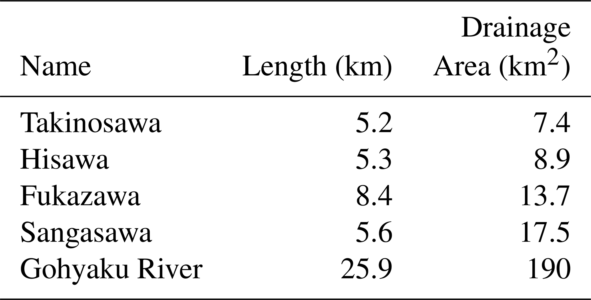
We investigated the tributaries of the Abukuma River near the Koriyama City in Fukushima, Japan (Fig. 1a), because in this region, studies on uplift and erosion rates have been extensively conducted (e.g., Tanaka et al., 1996; Matsushi et al., 2014; Fukuda et al., 2020). The Abukuma River drains the Nakadori area in Fukushima, draining an area of 5400 km² and being 239 km in length. The study area is about 150 km from the river mouth, located in the west of the Koriyama City. Five tributaries, Takinosawa, Hisawa, Fukazawa, Sangasawa, and Gohyaku River, were surveyed. Four of these tributaries (Takinosawa, Hisawa, Fukazawa, and Sangasawa) join the Gohyaku River, which merges into the mainstream of the Abukuma River (Fig. 1c, Table 1). These rivers are all bedrock rivers where the channel floor is partially covered with gravel.

The study area is in the forearc region of the Northeastern Japan Arc, which is bounded by the Tanakura tectonic line from the Southwestern Japan Arc (Ichikawa, 1990). A gentle synclinal structure with an NNE-SSW trending fold axis exists in this area, where the strata dip <20–40°. Several North-South trending faults are distributed in this study region, although they are inactive faults (Kubo et al., 2003; Yamamoto and Sakaguchi, 2023).

The bedrock of the study area is composed of metamorphic rocks, Cretaceous igneous rocks, Middle Miocene sedimentary rocks, and Late Miocene pyroclastic and volcanic rocks. The metamorphic rocks are composed of muscovite-biotite-plagioclase-quartz gneiss, distributed in the central region of the study area. Formation age is unknown. The Lower Cretaceous Abukuma granitic rocks, consisting of granodiorite (Kubo et al., 2003) in the surveyed area, are distributed in the northern region of the study area. The Middle Miocene Horiguchi Formation, consisting of marine sedimentary rocks, is distributed in the southwestern region of the study area (Yamamoto and Sakaguchi, 2023). Massive sandstones and alternating beds of parallel-laminated sandstones and siltstones occur in this formation. The Late Miocene Kogyoku Formation is composed mainly of pyroclastic deposits filling the Kogyoku Caldera. They are distributed in the northeastern region of the study area (Yamamoto and Sakaguchi, 2023). Dacite, lapilli tuff, and tuff breccia occur in the formation. In addition to these units, intrusive dacites and andesites occur in both igneous and sedimentary sequences.

Various studies implied that the rock uplift, exhumation, and denudation rates of the Abukuma River drainage basin are lower than those of adjacent regions. Based on geomorphic analyses, Fujiwara et al. (2005) estimated the average rock uplift rate of the Abukuma basin to be 0–0.3 mm yr⁻¹ over the past 100 kyr. This estimate was derived from the relative heights of fluvial terrace surfaces formed during the Last Interglacial and the preceding glacial period (Yoshiyama and Yanagida, 1995; Tanaka et al., 1996), combined with interpolation of uplift rates from surrounding areas (Fujiwara et al., 2004). Longer-term exhumation rates of this region were constrained using apatite and zircon (U-Th)/He thermochronometry. Applying this method to Cretaceous granitic rocks in the Abukuma Mountains, Fukuda et al. (2020) estimated Myr-scale exhumation rates of approximately 0.02–0.03 mm yr⁻¹. In addition, terrestrial cosmogenic nuclide analyses indicated denudation rates of 0.076–0.124 mm yr⁻¹ for the Abukuma River drainage basin (Matsushi et al., 2014).

In contrast, the Ou Backbone Range, which forms the tectonic core of the northeastern Japan Arc, exhibits substantially higher exhumation rates of approximately 0.1–1.5 mm yr⁻¹ (Fukuda et al., 2020). These values are roughly an order of magnitude greater than those estimated for the Abukuma River basin. Collectively, these studies demonstrate that the Abukuma River basin has experienced relatively low uplift and erosion rates compared with adjacent mountainous regions.

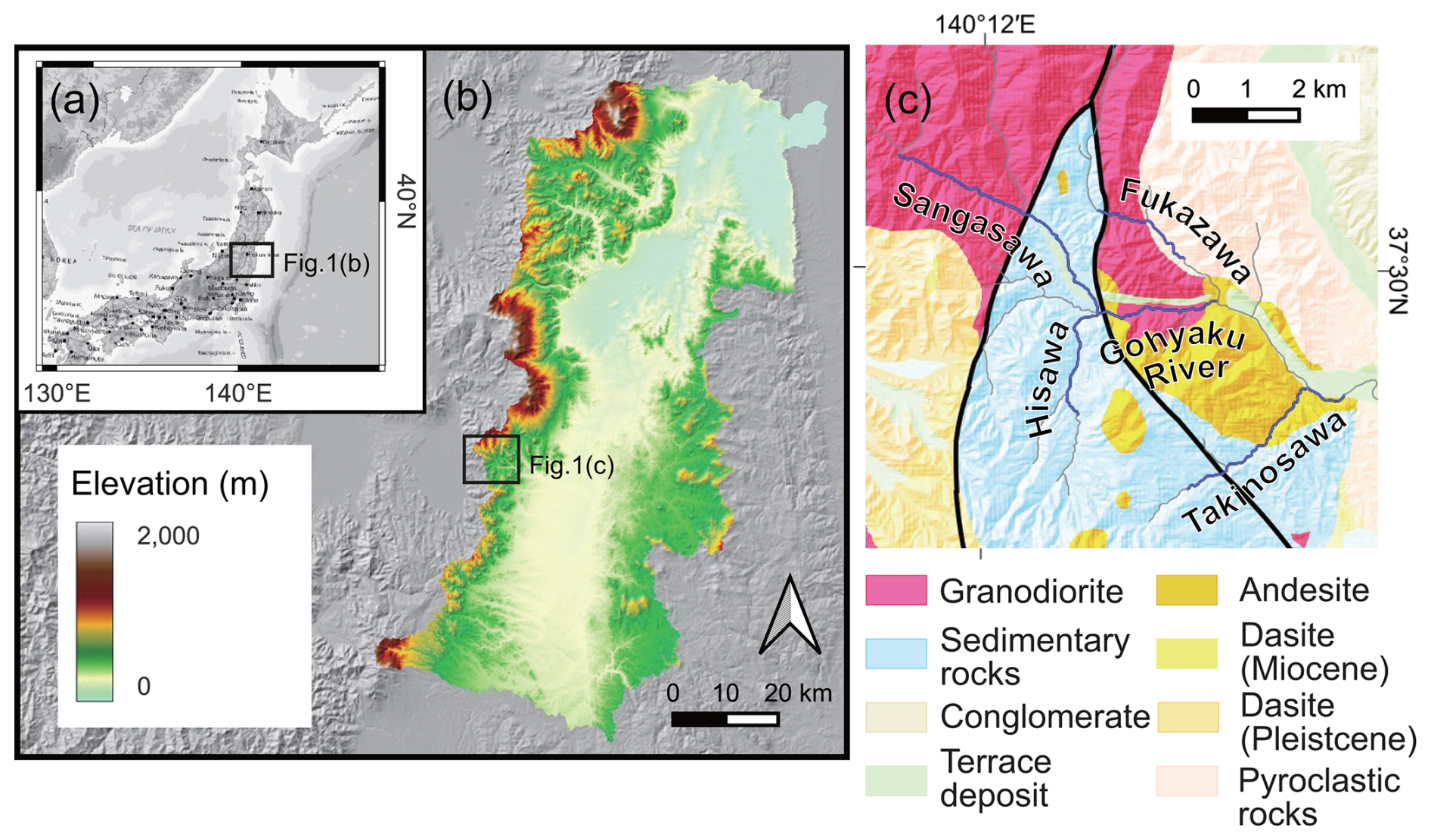
Figure 1 Index map and surveyed areas. The map data were obtained from the Technical Report of the Geospatial Information Authority of Japan. (a) Location of the Abukuma River basin. (b) Map of the Abukuma basin. The topographic elevation is exhibited in colors. (c) Geological map with surveyed tributaries. Black lines indicate major faults, and blue lines indicate the researched tributaries.

Table 1 Tributary information. Takinosawa, Hisawa, Fukazawa, and Sangasawa are tributaries of Gohyaku River.

3 River incision model

Numerous bedrock incision models have been proposed not only to understand the formative mechanisms resulting in the formation of bedrock river profiles (e.g., Sklar and Dietrich, 1998, 2004; Whipple and Tucker, 1999; Inoue et al., 2014; Aubert et al., 2016) but also to estimate the crustal uplift rates of mountainous regions (e.g., Howard, 1994; Pritchard et al., 2009; Roberts et al., 2012). In those models, the following formulation was utilized to represent bedrock river elevation change in the area experiencing continuous rock uplift:

$$\begin{array}{}\text{(1)}& {\displaystyle \frac{\partial \mathit{\eta }}{\partial t}}=U-E\end{array}$$

where η denotes surface elevation, U and E are the rock uplift and bedrock erosion rates, respectively. At steady state, the left side of Eq. (1) equals zero, and thus rock uplift is balanced by surface erosion.

Among various incision models (e.g., Howard and Kerby, 1983; Seidl and Dietrich, 1992; Tucker and Slingerland, 1994; Sklar and Dietrich, 2004; Lamb et al., 2008; Shobe et al., 2017), this study examined the sediment-flux-dependent model (SFDM) and two types of stream power models (Sklar and Dietrich, 2004; Chatanantavet and Parker, 2009; Inoue et al., 2017; Campforts et al., 2020; Guryan et al., 2024) to assess how well they capture the actual responses of bedrock rivers to variations in bedrock strength. In SFDM (Sklar and Dietrich, 2004; Whipple and Tucker, 2002), abrasion-saltation processes are explicitly represented as the dominant mechanism of bedrock incision (Sklar and Dietrich, 2004). This model considers that the flux of the impact kinetic energy of transported sediment particles determines the incision rate. The stream power models consider that the bedrock incision rates are proportional to the loss of the stream energy per unit time and area (i.e., stream power) (Howard, 1994). The formulations of these models are described in detail below.

3.1 Sediment-flux-dependent model

In the sediment-flux-dependent model (Sklar and Dietrich, 2004), the incision rate E [m s⁻¹] is obtained by:

$$\begin{array}{}\text{(2)}& E=V_{\mathrm{i}}{I}_{\mathrm{r}}(\mathrm{1}-P_{\mathrm{c}})\end{array}$$

in which V_i is the average volume of bedrock detached per particle impact, I_r is the rate of particle impacts per unit area per unit time, and P_c is the fraction of the covered riverbed.

Assuming the bedrock to be an elastic brittle material, V_i can be rewritten by the classic impact wear model of Bitter (1963) as:

$$\begin{array}{}\text{(3)}& V_{\mathrm{i}}={\displaystyle \frac{\mathrm{1}/\mathrm{2}{M}_{\mathrm{p}}(U_{\mathrm{i}}\sin \mathit{\alpha }{)}^{\mathrm{2}}}{{\mathit{\epsilon }}_{\mathrm{v}}}}\end{array}$$

where M_p [kg] denotes particle mass. U_i [m s⁻¹] indicates the impact velocity of the particle, and α is the saltation angle. The parameter ε_v [J] denotes the total energy required to erode a unit volume of rock (Sklar and Dietrich, 2004). The threshold energy ε_v is calculated by (Engle, 1978; Sklar and Dietrich, 2001):

$$\begin{array}{}\text{(4)}& {\mathit{\epsilon }}_{\mathrm{v}}={\displaystyle \frac{k_{\mathrm{v}}{\mathit{\sigma }}_{\mathrm{t}}^{\mathrm{2}}}{\mathrm{2}Y}}\end{array}$$

where σ_t [MPa] is bedrock tensile strength, and k_v denotes rock resistance coefficient. Y [MPa] represents Young's modulus. By substituting Eq. (4) into Eq. (3), we obtain:

$$\begin{array}{}\text{(5)}& V_{\mathrm{i}}={\displaystyle \frac{\mathit{\pi }{\mathit{\rho }}_{\mathrm{s}}{D}_{\mathrm{s}}^{\mathrm{3}}{w}_{\mathrm{s}i}^{\mathrm{2}}Y}{\mathrm{6}{k}_{\mathrm{v}}{\mathit{\sigma }}_{\mathrm{t}}^{\mathrm{2}}}}\end{array}$$

where ρ_s [kg m⁻³] and D_s [m] denote the density of sediment and the diameter of a spherical sediment grain, respectively. $M_{\mathrm{p}}={\mathit{\rho }}_{\mathrm{s}}\mathit{\pi }{D}_{\mathrm{s}}^{\mathrm{3}}/\mathrm{6}$ is the mass of a spherical grain, and w_si [m s⁻¹] is the vertical component of the particle velocity on impact (i.e., w_si=U_isin α).

Here, the number of particle impacts per unit time and area I_r is proportional to the flux of the bedload particles and inversely proportional to the downstream distance between the impacts. Using the sediment flux volume per unit width q_s [m² s⁻¹] and the saltation hop length L_s [m], I_r is expressed as:

$$\begin{array}{}\text{(6)}& I_{\mathrm{r}}={\displaystyle \frac{{\mathit{\rho }}_{\mathrm{s}}{q}_{\mathrm{s}}}{M_{\mathrm{p}}{L}_{\mathrm{s}}}}.\end{array}$$

Substituting $M_{\mathrm{p}}={\mathit{\rho }}_{\mathrm{s}}\mathit{\pi }{D}_{\mathrm{s}}^{\mathrm{3}}/\mathrm{6}$ into Eq. (6),

$$\begin{array}{}\text{(7)}& I_{\mathrm{r}}={\displaystyle \frac{\mathrm{6}}{\mathit{\pi }{D}_{\mathrm{s}}^{\mathrm{3}}}}{q}_{\mathrm{s}}{\displaystyle \frac{\mathrm{1}}{L_{\mathrm{s}}}}.\end{array}$$

Substituting Eqs. (5) and  (7) into Eq. (2), bedrock incision rate E is recast as:

$$\begin{array}{}\text{(8)}& E={\displaystyle \frac{{\mathit{\rho }}_{\mathrm{s}}{w}_{\mathrm{s}i}^{\mathrm{2}}Y}{L_{\mathrm{s}}{k}_{\mathrm{v}}{\mathit{\sigma }}_{\mathrm{t}}^{\mathrm{2}}}}{q}_{\mathrm{s}}(\mathrm{1}-P_{\mathrm{c}}).\end{array}$$

Chatanantavet and Parker (2009) proposed that the abrasion coefficient can be defined as:

$$\begin{array}{}\text{(9)}& \mathit{\beta }={\displaystyle \frac{{\mathit{\rho }}_{\mathrm{s}}{w}_{\mathrm{s}i}^{\mathrm{2}}Y}{L_{\mathrm{s}}{k}_{\mathrm{v}}{\mathit{\sigma }}_{\mathrm{t}}^{\mathrm{2}}}}.\end{array}$$

Using this formulation, Eq. (8) can be rewritten as:

$$\begin{array}{}\text{(10)}& E=\mathit{\beta }{q}_{\mathrm{s}}(\mathrm{1}-P_{\mathrm{c}}).\end{array}$$

Based on the flume experiments in the field scale, Inoue et al. (2014, 2017) pointed out that the erosion rate is proportional to the square root of the grain size rather than the shear stress and that it does not significantly depend on the Young's modulus. From this experimental result, Inoue et al. (2017) proposed the following relation:

$$\begin{array}{}\text{(11)}& E={\mathit{\beta }}_{\mathrm{0}}{\mathit{\sigma }}_{\mathrm{t}}^{\mathrm{2}}{\left({\displaystyle \frac{D_{\mathrm{s}}}{k_{\mathrm{s}}}}\right)}^{\mathrm{0.5}}{q}_{\mathrm{s}}(\mathrm{1}-P_{\mathrm{c}})\end{array}$$

where β₀ is an empirical coefficient (=0.0001) [kg² m⁻³ s⁻⁴], k_s [m] represents the height of the hydraulic roughness, which is defined by the equation k_s=κ_aP_c + κ_b(1−P_c). Here, κ_a is a roughness coefficient that is linear to the grain diameter D_s, and κ_b is a constant representing the bedrock roughness. In Inoue et al. (2014), κ_a=2.5D_s and κ_b=0.0032. We adopted these relations and values in the model calculation.

The bedrock covered ratio P_c can be expressed in various ways; however, in this study, it is defined as:

$$\begin{array}{}\text{(12)}& P_{\mathrm{c}}={\displaystyle \frac{q_{\mathrm{s}}}{q_{\mathrm{t}}}}\end{array}$$

following the work of Sklar and Dietrich (2004). The sediment transport capacity q_t [m² s⁻¹] takes the form (Meyer-Peter and Müller, 1948; Fernandez Luque and Van Beek, 1976):

$$\begin{array}{}\text{(13)}& q_{\mathrm{t}}=\mathrm{5.7}{\left(R_{\mathrm{b}}g{D}_{\mathrm{s}}^{\mathrm{3}}\right)}^{\mathrm{1}/\mathrm{2}}{\left({\mathit{\tau }}^{\ast }-{\mathit{\tau }}_{\mathrm{c}}^{\ast }\right)}^{\frac{\mathrm{3}}{\mathrm{2}}}\end{array}$$

where R_b denotes the nondimensional buoyant density of the sediment ($R_{\mathrm{b}}=({\mathit{\rho }}_{\mathrm{s}}-{\mathit{\rho }}_{\mathrm{w}})/{\mathit{\rho }}_{\mathrm{w}}$). The parameters ρ_w [kg m⁻³] and g [m s⁻²] denote the water density and gravity acceleration, respectively. The Shields stress τ^∗, which is the nondimensional bed shear stress, is defined as:

$$\begin{array}{}\text{(14)}& {\mathit{\tau }}^{\ast }={\displaystyle \frac{{\mathit{\tau }}_{\mathrm{b}}}{\left({\mathit{\rho }}_{\mathrm{s}}-{\mathit{\rho }}_{\mathrm{w}}\right)g{D}_{\mathrm{s}}}}\end{array}$$

where τ_b is the bed shear stress. The critical Shields number ${\mathit{\tau }}_{\mathrm{c}}^{\ast }$ is the value of τ^∗ at the threshold of particle motion, which was regarded as constant (0.03) for simplicity.

Assuming that the stream flows in a uniform steady condition, the bed shear stress τ_b is calculated as (Chatanantavet and Parker, 2009):

$$\begin{array}{}\text{(15)}& {\mathit{\tau }}_{\mathrm{b}}={\mathit{\rho }}_{\mathrm{w}}{C}_{\mathrm{f}}^{\mathrm{1}/\mathrm{3}}{g}^{\mathrm{2}/\mathrm{3}}{\left({\displaystyle \frac{Q_{\mathrm{w}}}{W}}\right)}^{\mathrm{2}/\mathrm{3}}{S}^{\mathrm{2}/\mathrm{3}}\end{array}$$

where C_f denotes the bed friction coefficient. Q_w [m³ s⁻¹] and W [m] represent the water discharge and the width of the river, respectively. S indicates the bed slope.

Water discharge Q_w is determined by the following equation (Whipple and Tucker, 1999):

$$\begin{array}{}\text{(16)}& Q_{\mathrm{w}}=k_{\mathrm{SFDM}}\stackrel{\mathrm{‾}}{P}A\end{array}$$

where k_SFDM is a discharge coefficient representing rainfall variability, and $\stackrel{\mathrm{‾}}{P}$ [m s⁻¹] denotes the average precipitation per unit area. A [m²] represents the drainage area. Because the amounts of precipitation causing bedrock erosion are expected to be significantly larger than the average condition, the discharge coefficient k_SFDM is also expected to be considerably greater than unity.

Assuming that the bedload sediment supply from the tributaries of the stream is proportional to the volume of the eroded material in the drainage area (Chatanantavet and Parker, 2009), the bedload discharge per unit width q_s domain is obtained as:

$$\begin{array}{}\text{(17)}& q_{\mathrm{s}}\left(x\right)={\displaystyle \frac{\mathrm{1}}{W\left(x\right)}}\left(q_{\mathrm{s}}\left(\mathrm{0}\right)W\left(\mathrm{0}\right)+a\int {\displaystyle \frac{\mathrm{d}A}{\mathrm{d}x}}E\left(x\right)\mathrm{d}x\right)\end{array}$$

where x [m] is the streamwise distance from the upstream end of the calculation domain, and q_s(0) is the bedload sediment supply at the upstream end. The ratio of the bedload to the total sediment supply is represented by a. In this study, we set a=0.14 based on a previous study of Takayama (1965).

The sediment supply per unit width at the upstream end is assumed to be in a steady state, where the erosion rate E_eq is equal to the uplift rate of the bedrock. The bedload sediment discharge q_s(0) at the upstream end (x=0) is written as:

$$\begin{array}{}\text{(18)}& q_{\mathrm{s}}\left(\mathrm{0}\right)={\displaystyle \frac{aA\left(\mathrm{0}\right)E_{\mathrm{eq}}}{W\left(\mathrm{0}\right)}}\end{array}$$

where A(0) and W(0) denote the drainage area and the channel width at the upstream end, respectively.

The channel width W is estimated by the empirical formulation using the river discharge (Finnegan et al., 2005) as follows:

$$\begin{array}{}\text{(19)}& W=k_{\mathrm{w}}{Q}_{\mathrm{w}}^{\mathrm{0.5}}\end{array}$$

where k_w is the uniquely determined coefficient for each tributary.

To calculate the steady-state (E=U) channel profiles, Eq. (11) was recast to solve for the channel slope S using Eqs. (1), (13), (14),  (15), and (19), which takes the form:

$$\begin{array}{}\text{(20)}& {\displaystyle }& {\displaystyle }{S}_{\mathrm{eq},\mathrm{SFDM}}=\left[{\displaystyle \frac{R_{\mathrm{b}}{g}^{\mathrm{1}/\mathrm{3}}{D}_{\mathrm{s}}{k}_{\mathrm{w}}^{\mathrm{2}/\mathrm{3}}}{C_{\mathrm{f}}^{\mathrm{1}/\mathrm{3}}{Q}_{\mathrm{w}}^{\mathrm{1}/\mathrm{3}}}}\mathit{\{}{\mathit{\tau }}_{\mathrm{c}}^{\ast }\right.\text{(21)}& {\displaystyle }& {\displaystyle }+{\left.{\left({\displaystyle \frac{{\mathit{\beta }}_{\mathrm{0}}{q}_{\mathrm{s}}^{\mathrm{2}}}{\mathrm{5.7}(R_{\mathrm{b}}g{)}^{\mathrm{1}/\mathrm{2}}{D}_{\mathrm{s}}\left({\mathit{\beta }}_{\mathrm{0}}{D}_{\mathrm{s}}^{\mathrm{1}/\mathrm{2}}{q}_{\mathrm{s}}-k_{\mathrm{s}}^{\mathrm{1}/\mathrm{2}}{\mathit{\sigma }}_{\mathrm{t}}^{\mathrm{2}}U\right)}}\right)}^{\mathrm{2}/\mathrm{3}}\mathit{\}}\right]}^{\mathrm{3}/\mathrm{2}}.\end{array}$$

3.2 Stream power models

We applied two types of the stream power model. One is the Area-based Stream Power Model (ASPM), which considers the lithologic strength of bedrock according to its lithologic types Campforts et al. (2020). This model does not account for the effect of the sediment cover ratio on the river bed. The other is the Stream Power with Alluvium Conservation and Entrainment Model (SPACEM) (Shobe et al., 2017; Guryan et al., 2024). SPACEM incorporates both lithologic strength and sediment cover ratio.

The ASPM is represented by the following equation:

$$\begin{array}{}\text{(22)}& E=k_{\mathrm{a}}{L}_{\mathrm{E}}{S}^n{A}^m\end{array}$$

where k_a (m^1−2 m yr⁻¹) is the erosional efficiency parameter excluding the influence of the erodibility of bedrock, and L_E is the relative erodibility of bedrock index. The positive exponents m and n are empirical parameters depending on lithology, rainfall variability, and sediment load (Whipple and Tucker, 1999; Campforts et al., 2020). The erosional efficiency k_a was determined by a Bayesian optimization in this study. L_E was determined using the value proposed in Campforts et al. (2020).

On the other hand, SPACEM considers lithology and sediment cover ratio but does not explicitly include sediment tool effects. This model considers the rates of erosion E_r [m yr⁻¹] and entrainment E_s [m yr⁻¹], which relate to the sediment thickness on the riverbed. The following equation represents the erosion rate E_r:

$$\begin{array}{}\text{(23)}& E_{\mathrm{r}}=K_{\mathrm{r}}{q}_{\mathrm{w},\mathrm{yr}}{S}^n{e}^{-H/H_{\ast }}\end{array}$$

where K_r [m^1−2 m yr⁻¹] is the bedrock erodibility, q_w,yr [m² yr⁻¹] is the mean annual water discharge per unit width, H [m] is the thickness of the sediment cover, and H_∗ [m] is the bedrock roughness scale. K_r reflects the bedrock strength. The entrainment rate of the sediment from the bed E_s is represented as:

$$\begin{array}{}\text{(24)}& E_{\mathrm{s}}=K_{\mathrm{sed}}{q}_{\mathrm{w},\mathrm{yr}}{S}^n\left(\mathrm{1}-e^{-H/H_{\ast }}\right)\end{array}$$

where K_sed [m^1−2 m yr⁻¹] denotes the sediment erodibility. In this model, the cover ratio P_c is determined as $H/H_{\ast }$. The sediment thickness H depends on the rate of sediment entrainment E_s and deposition D_s, so that the relationship is calculated as:

$$\begin{array}{}\text{(25)}& (\mathrm{1}-\mathit{\varphi }){\displaystyle \frac{\partial H}{\partial t}}=D_{\mathrm{s}}-E_{\mathrm{s}}={\displaystyle \frac{q_{\mathrm{s}}}{q_{\mathrm{w},\mathrm{yr}}}}{W}_{\mathrm{s}}-E_{\mathrm{s}}\end{array}$$

where ϕ and q_s denote the sediment porosity and the sediment flux per unit width, respectively. W_s is the grain settling velocity determined by the grain size D_s. In this study, q_s was calculated using Eq. (17). The mean annual water discharge q_w,yr was calculated using mean annual precipitation rate ${\stackrel{\mathrm{‾}}{P}}_{\mathrm{yr}}$ as follows:

$$\begin{array}{}\text{(26)}& q_{\mathrm{w},\mathrm{yr}}={\displaystyle \frac{k_{\mathrm{SPACEM}}{\stackrel{\mathrm{‾}}{P}}_{\mathrm{yr}}A}{W}}\end{array}$$

where k_SPACEM denotes a discharge coefficient representing rainfall variability.

Assuming the steady-state (E=U), the channel slopes can be calculated in the same manner as SFDM:

$$\begin{array}{}\text{(27)}& S_{\mathrm{eq},\mathrm{SPACEM}}={\left({\displaystyle \frac{q_{\mathrm{s}}{W}_{\mathrm{s}}}{K_{\mathrm{sed}}{q}_{\mathrm{w},\mathrm{yr}}^{\mathrm{2}}}}+{\displaystyle \frac{U}{q_{\mathrm{w},\mathrm{yr}}{K}_{\mathrm{r}}}}\right)}^{\mathrm{1}/n}\end{array}$$

In this calculation, the grain settling velocity W_s was assumed to be spatially constant in this model.

The value of K_r for the most fragile rock type (i.e., tuff) was set to $\mathrm{1.0}\times {\mathrm{10}}^{-\mathrm{5}}$ according to Guryan et al. (2024). Assuming that this coefficient is proportional to the rock tensile strength, the bedrock erodibility K_r,i for the ith rock type was determined as follows:

$$\begin{array}{}\text{(28)}& K_{\mathrm{r},i}={\displaystyle \frac{{\mathit{\sigma }}_{\mathrm{t},i}{K}_{\mathrm{r},\mathrm{tuff}}}{{\mathit{\sigma }}_{\mathrm{t},\mathrm{tuff}}}}\end{array}$$

where σ_t,i and σ_t,tuff denote the tensile strengths of the ith rock type and tuff, respectively.

3.3 Optimization of model parameters

In this study, the discharge coefficient k_SFDM, k_SPACEM, channel width coefficient k_w, and erosional coefficient (k_a) were optimized to minimize the elevation differences between the actual river profile and the result of the model calculation. The objective function was defined as the root mean square (RMS) of the total elevation differences summed over the 5 tributaries.

$$\begin{array}{}\text{(29)}& \mathrm{RMS}=\sqrt{{\displaystyle \frac{\mathrm{1}}{\mathrm{NM}}}\sum _{n,m=\mathrm{1}}^{\mathrm{NM}}\left(z_{n,m}^{\mathrm{O}}-z_{n,m}^{\mathrm{C}}\right)}\end{array}$$

$z_{n,m}^{\mathrm{O}}$ and $z_{n,m}^{\mathrm{C}}$ represent the observed and calculated elevation, respectively. The optimal parameters were determined using Optuna (Akiba et al., 2019), which is an optimization framework based on Bayesian optimization, a method that efficiently explores the optimal solution by sequentially updating the posterior distribution based on the evaluation results of a probabilistic model.

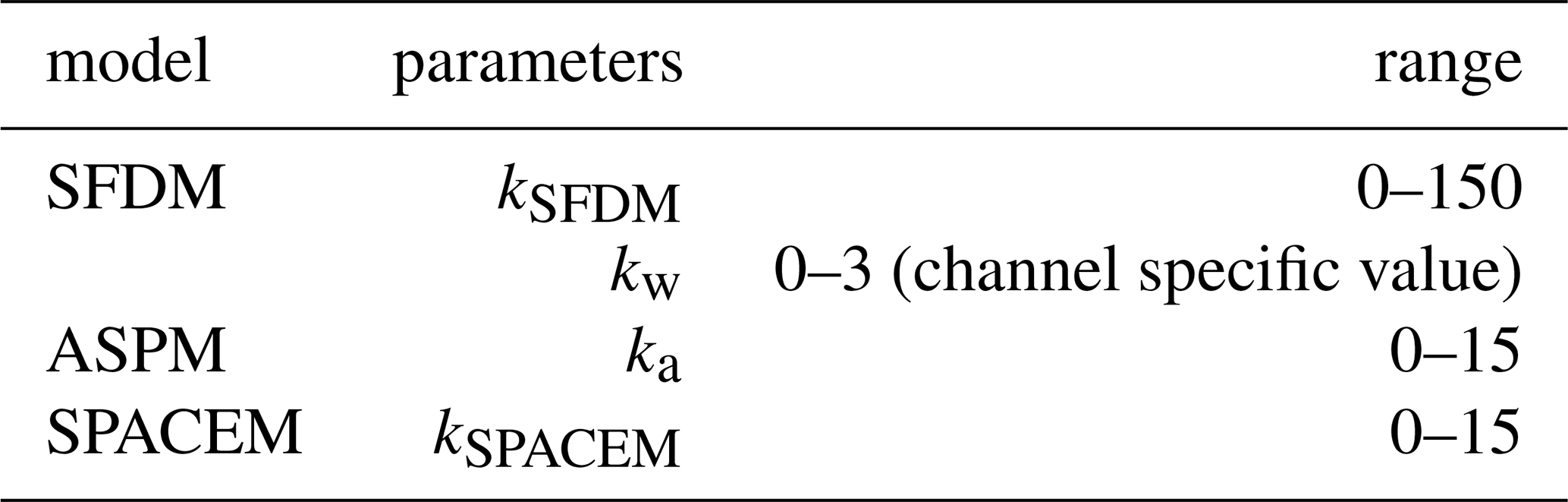
This study performed the Bayesian optimization with 10 000 trials to fit the model outputs to the observed river longitudinal profiles. As a result, the optimal parameters were obtained: k_SFDM and k_w for SFDM, k_a for ASPM, and k_SPACEM for SPACEM. In the case of SFDM, k_w was individually optimized for each tributary, while the remaining parameters were treated as common values across all tributaries. The search ranges for these parameters are summarized in Table 2. Note that the uncertainties associated with the optimized parameters were not explicitly evaluated in this analysis.

In addition, we performed a sensitivity analysis of the parameters used in SFDM, ASPM, and SPACEM that were adopted from the literature. Each parameter was varied within a reasonable range (Table 2), and the model was re-optimized for each parameter set using Bayesian optimization with Optuna to minimize the RMS error between the observed and calculated topography of the Gohyaku River.

Table 2 A list of optimized parameters and their searched ranges.

4 Methods for topographic and geologic analysis

4.1 Topographic analysis

The topographic elevation, slope, and drainage area along the channels of the surveyed rivers were extracted from the digital elevation model (DEM) of the Geospatial Information Authority of Japan. First, 10-m-mesh DEM data of the surveyed tributaries were utilized to calculate the flow accumulation. The Deterministic 8 algorithm, in which water at each pixel is assumed to flow in the direction of maximum downslope gradient, was employed to obtain the drainage areas (O'Callaghan and Mark, 1984). Flow paths draining more than 7×10⁴ km² were regarded as river channels. The channel slope was then calculated along the channel path from the elevation data. The geographical information system software SAGA GIS was used for these procedures (Conrad et al., 2015).

The normalized steepness index k_sn was used to clarify the effect of the bedrock strength on the channel steepness in all the investigated tributaries. This parameter is defined as the upstream area-weighted channel gradient (Campforts et al., 2020; Wobus et al., 2006):

$$\begin{array}{}\text{(30)}& k_{\mathrm{sn}}=S{A}^{\mathit{\theta }}\end{array}$$

The exponent θ is the concavity index. Empirical studies show that concavity indices typically range from 0.3 to 0.7 (Tucker and Whipple, 2002; Goren and Shelef, 2024). In this study, we adopted a value of 0.36, which was optimized for the study area.

Chi plots are commonly used to assess whether uplift rate and bedrock erodibility are spatially uniform (Perron and Royden, 2013). Under steady-state conditions with uniform erodibility, river profiles are linear in chi space; deviations from linearity indicate spatial variations in uplift rate or erodibility. It is a coordinate transformation to linearize the river profile determined by:

$$\begin{array}{}\text{(31)}& \mathit{\chi }=\underset{X_{\mathrm{b}}}{\overset{X}{\int }}{\left({\displaystyle \frac{A_{\mathrm{0}}}{A\left(x\right)}}\right)}^{m/n}\mathrm{d}X\end{array}$$

where X is the distance from downstream, and x_b is a base level. A₀ denotes a reference drainage area, and the drainage area at the downstream end is set in this study.

4.2 Measurement of Rock Strength

The lithologies of the bedrock were distinguished in the field survey and were recorded in the geological route map of the researched tributaries. The 1:50 000 and 1:200 000 geologic maps published by the Geological Survey of Japan were also used to distinguish the lithologies where the bedrock was not exposed on the channels.

Then, the tensile strengths of the various bedrock materials of the representative lithologies were sampled and measured using the Brazilian tension splitting test (Vutukuri et al., 1974). Before the analysis, the specimens were submerged in the water under a vacuum for 12 weeks until their weight did not change. This procedure was selected because the goal was to measure the bedrock strength in a wet condition. We justify this approach because it has been shown that the water content in the pore space of bedrock can affect the rock tensile strength (Bao et al., 2021).

In this test, the specimens had a diameter of 50 mm and a length of 25 mm (The Japanese Geotechnical Society, 2016). The load was applied to the specimen at 1 µm s⁻¹ until a crack formed, and the maximum load P_max [kN] at the moment of failure was measured.

The tensile strength σ_t was then determined using the following Eq. (32).

$$\begin{array}{}\text{(32)}& {\mathit{\sigma }}_{\mathrm{t}}={\displaystyle \frac{\mathrm{2}{P}_{\max }}{\mathit{\pi }DL}}\times \mathrm{1000}\end{array}$$

where D (mm) and L denote the diameter and length of the specimen, respectively.

The gneissosity planes in gneiss can result in large variability depending on the surface on which the failure occurred. We assumed that the riverbed failure occurred along the weak plane, so we adopted not the average value, but the value when the specimen was cropped along the weak plane.

4.3 Automated grain size measurements of riverbed gravels

The grain sizes of the riverbeds were measured from drone-derived 3D point cloud data. In recent years, the methods for automated grain-size analysis have been rapidly developing (e.g., Soloy et al., 2020; Steer et al., 2022; Mair et al., 2024). Among those studies, the method proposed by Steer et al. (2022) can measure the three axes of the grains from 3D point cloud data obtained by drone photogrammetry, allowing the grain axes lengths and the volume of grains to be measured. In this study, we adopted the volume-based metric for the representative grain size, so that the G3Point method Steer et al. (2022) was employed.

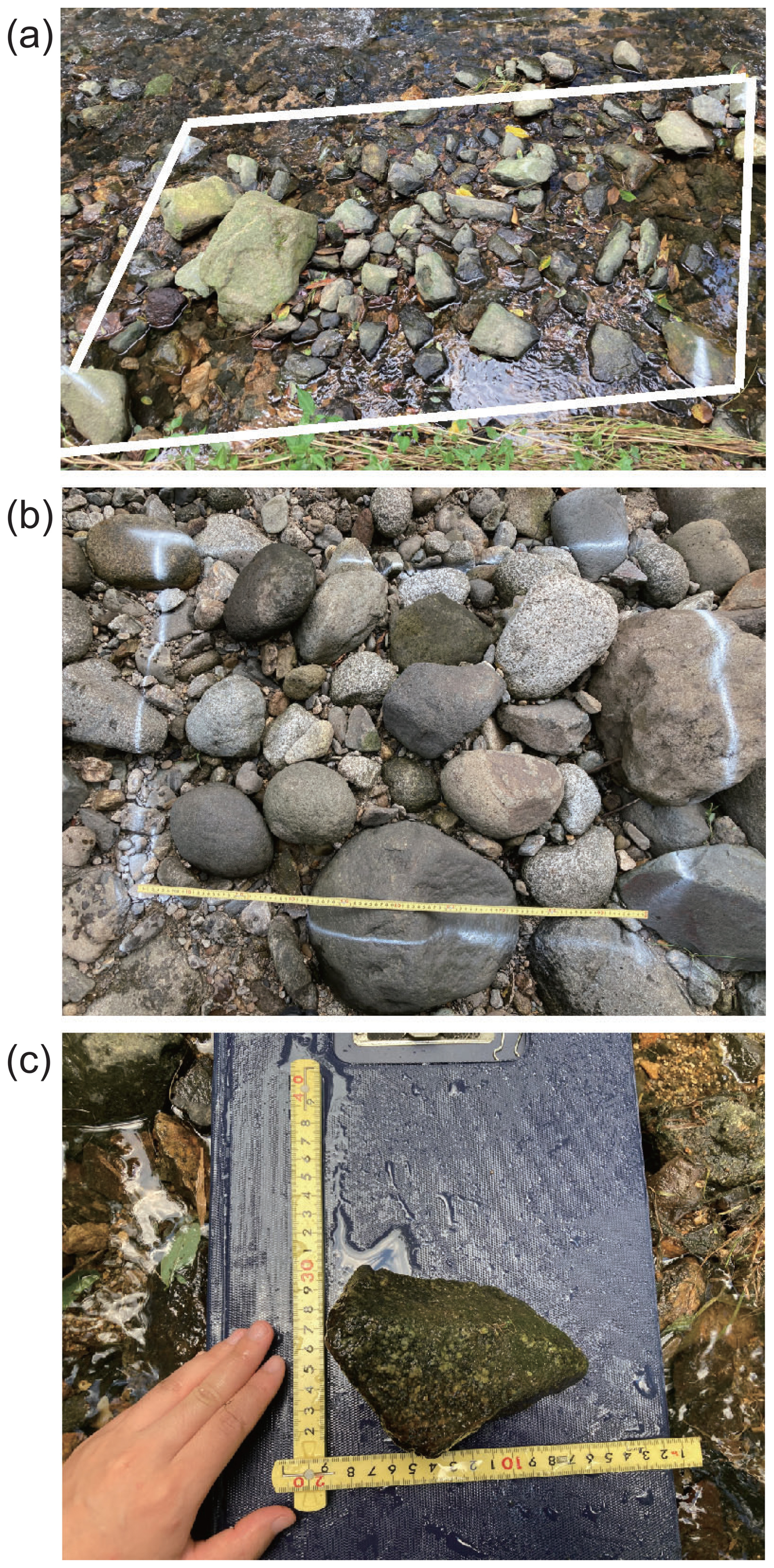
Figure 2 Photos of river gravels. (a) Photograph of gravels at Sakura River, the Tamura-Country, Fukushima. The area surrounded by the white lines was about 1.0 × 2.5 m. (b) Photograph of gravel at Gohyaku River, the Koriyama City, Fukushima. The area size was 0.8 m × 1.0 m. (c) Manually measuring gravel size.

The measurement procedures were as follows. (1) The drone (DJI Air-2s) photographed approximately 100–200 m² areas of the riverbeds. (2) 3D point clouds exhibiting riverbed surface morphologies were produced by the Structure from Motion algorithm using Agisoft Metashape. (3) Triaxial ellipsoids fitted the morphology of each gravel to measure the diameters of the grains using the software G3Point (Steer et al., 2022).

In this study, we defined the representative grain diameter ${\stackrel{\mathrm{‾}}{D}}_{\mathrm{s}}$ as the mean of the diameter of the spheres in the weighted arithmetic mean (D₅₀), which are equal to the fitted tri-axial ellipsoids in volume.

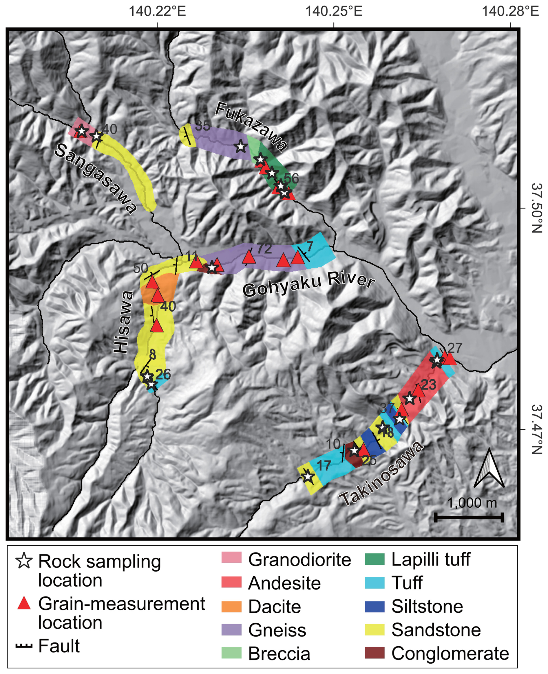
Figure 3 Route map in the researched area. The classification of lithologic distributions in the unsurveyed areas was inferred from previous studies (Kubo et al., 2003; Yamamoto and Sakaguchi, 2023). The star mark represents the location of the rock sampling. The pink triangle represents the location where the grain size distributions were measured using the drone. DEM data were obtained from the Technical Report of the Geospatial Information Authority of Japan.

Since the G3Point program can analyze a maximum of 1 million points at a time, we split the analysis area into two or three non-overlapping rectangular regions with a width of 5 m or less. The mean values of these subareas were then used as the results of the measurements in the surveyed area. We cropped the water surface contained in the 3D point cloud manually because G3Point sometimes misidentified the water surface as the grain surface. In the G3Point method, 10 points are required to fit an ellipsoid to a grain, so the measurable minimal grain size is 1–2 cm.

To estimate the mean diameter D_s of the riverbed gravels along each stream, the measured values were interpolated with Sternberg's law Eq. (33) (Sternberg, 1875; Snelder et al., 2011; Miller et al., 2014):

$$\begin{array}{}\text{(33)}& D_x=D_{\mathrm{0}}\exp \left(-{\mathit{\alpha }}_{\mathrm{d}}x\right)\end{array}$$

where D₀ is the grain diameter at the origin, and α_d is the change rate of the mean diameter. Here, we assumed that the river gravels fine downstream (Parker, 1991), so that α_d should be a positive value. These parameters D₀ and α_d were estimated from the mean of the measured values using the least-squares method.

The grain sizes of the riverbed gravels were also measured manually at two locations (Sakura River and Gohyaku River) to evaluate the accuracy of the automated measurements (Fig. 2). In this manual measurement, the longest (a), intermediate (b), and shortest (c) axes were measured. First, we delineated a several-square-meter area on a river bar using spray paint. Within this area, we measured the sizes of clasts that were visually identifiable from a vertical viewpoint, had exposed surfaces, and possessed a short axis of at least 1 cm. Then the results were compared with those obtained by the G3Point program.

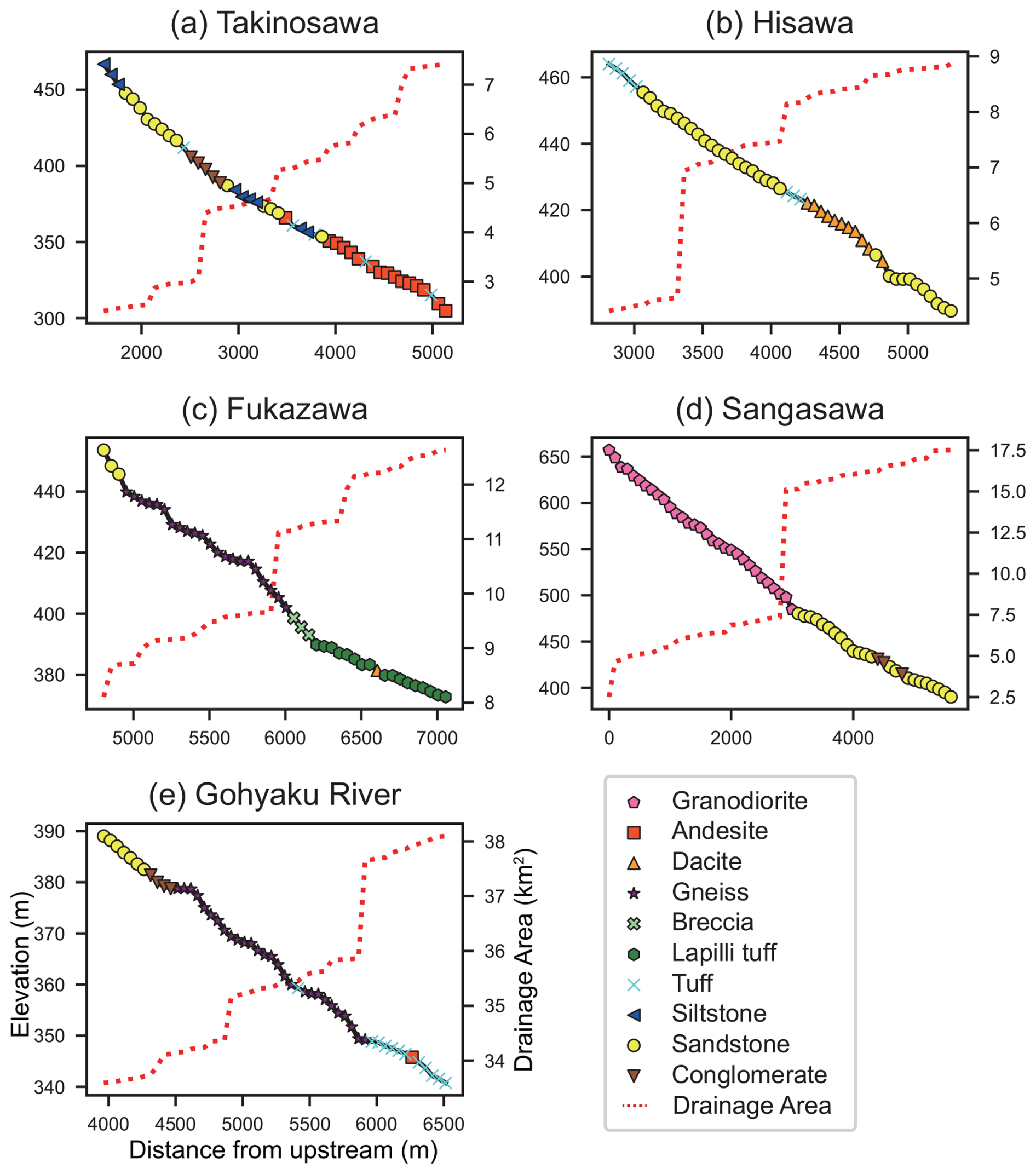
Figure 4 River profiles extracted from the DEM and the lithology data obtained through field surveys – the point on the channel positioned at 10-m intervals. The upstream end was at the channel's endpoint on the map.

5 Results

5.1 Topography and geology of the surveyed channels

We identified ten types of sedimentary, pyroclastic, gneiss, and igneous rocks exposed on the riverbed of five tributaries of the Abukuma River (Takinosawa, Hisawa, Fukazawa, Sangasawa, and Gohyaku Rivers) (Fig. 3). The sedimentary rock is subdivided into conglomerate, massive sandstone, and siltstone. The pyroclastic rocks include volcanic breccia, lapilli tuff, and tuff. The igneous rocks are granodiorite and andesite. The volcanic and pyroclastic rocks are distributed in the northeastern region where Takinosawa and Fukazawa exist. The granodiorite is exposed in the northwestern region (Sangasawa). A major fault exists in the upstream region of Gohyaku River, while no significant topographic change at the fault was observed in the field. A gentle synclinal structure with an NNE-SSW trending fold axis was observed in the study area, whereas an anticlinal structure was also observed upstream of Takinosawa and a further one in a south tributary. These clinal structures were all trending NNE-SSW.

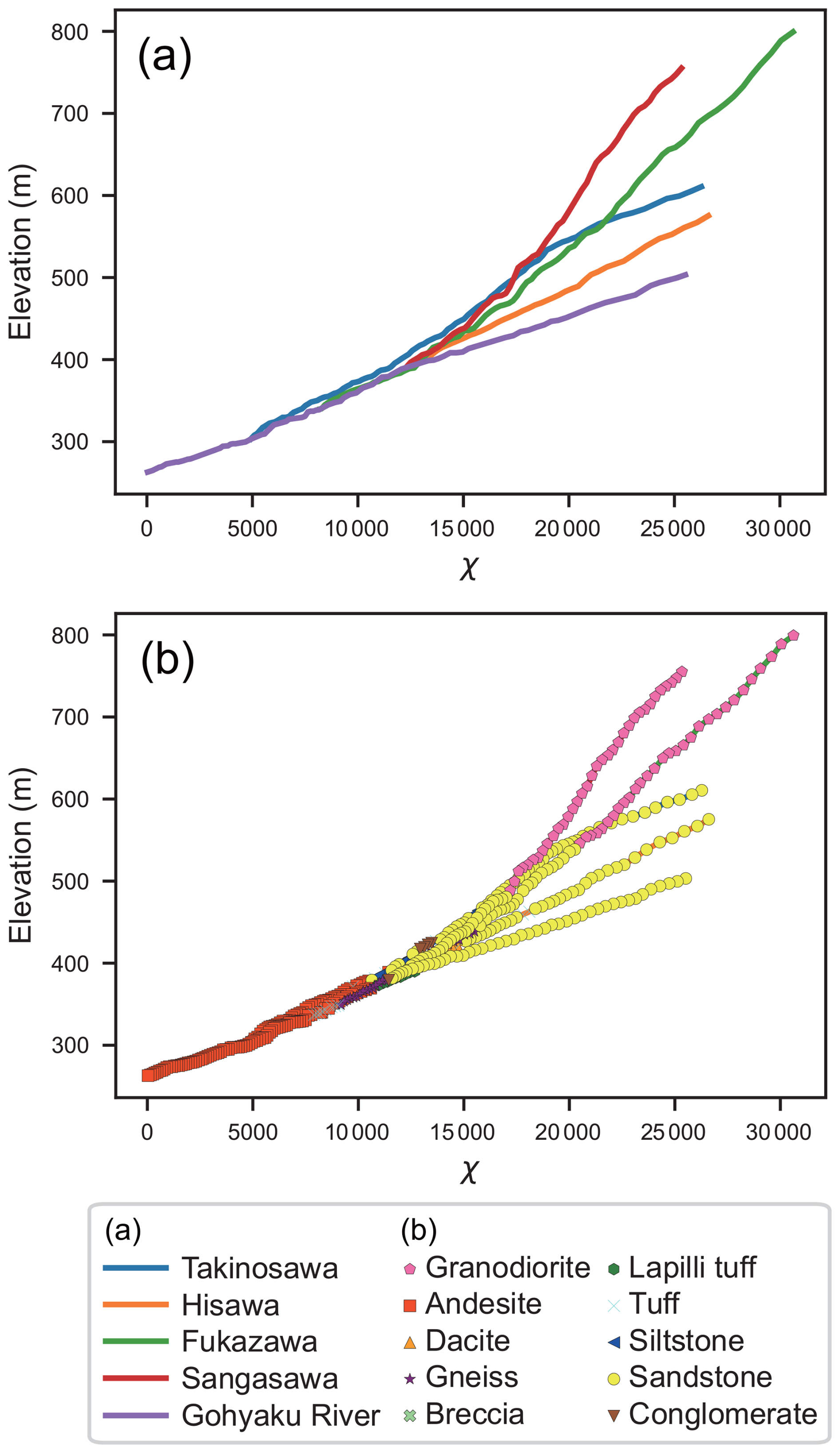
Figure 5 Channel profiles represented as chi plots. The x-axis represents the chi value calculated using Eq. (31). In this study, the concavity index $m/n$ was assumed to be 0.36 for constructing the chi plots. (a) Chi plots of individual tributaries. (b) Chi plots of individual tributaries colored by lithology.

The results of topographic analysis and geological survey indicated that the river profiles did not vary significantly in slope at the lithologic boundaries. The river course does not show significant changes at fault or fold locations, suggesting that tectonic structures exert limited control on channel morphology in this area. Figure 4 exhibits the channel longitudinal profiles of the surveyed tributaries extracted from the DEM, where the lithologies identified through the field surveys were plotted as symbols and colors. Most of the rivers have weakly concave-upward smooth profiles. The channel slopes in the surveyed region range from 0.02 to 0.05.

Several knickpoints are associated with lithological boundaries. In Takinosawa, a knickpoint occurs at the boundary between sandstone and conglomerate, with a thin tuff layer in between. The average channel slope in the conglomerate reach is 0.056, whereas that in the upstream sandstone reach is 0.052, yielding a slope difference of only 0.004 across the lithologic boundary. Other minor knickpoints that coincide with lithological boundaries exhibit a trend opposite to the commonly expected pattern, in which channel gradients are steeper in harder bedrock and gentler in weaker lithologies. In Fukazawa, knickpoints occur at both the sandstone-gneiss and breccia-tuff boundaries. However, in both cases, softer rocks (sandstone and breccia) are located upstream, where channel slopes are steeper, whereas harder rocks (gneiss and lapilli tuff) occur downstream, where slopes are lower.

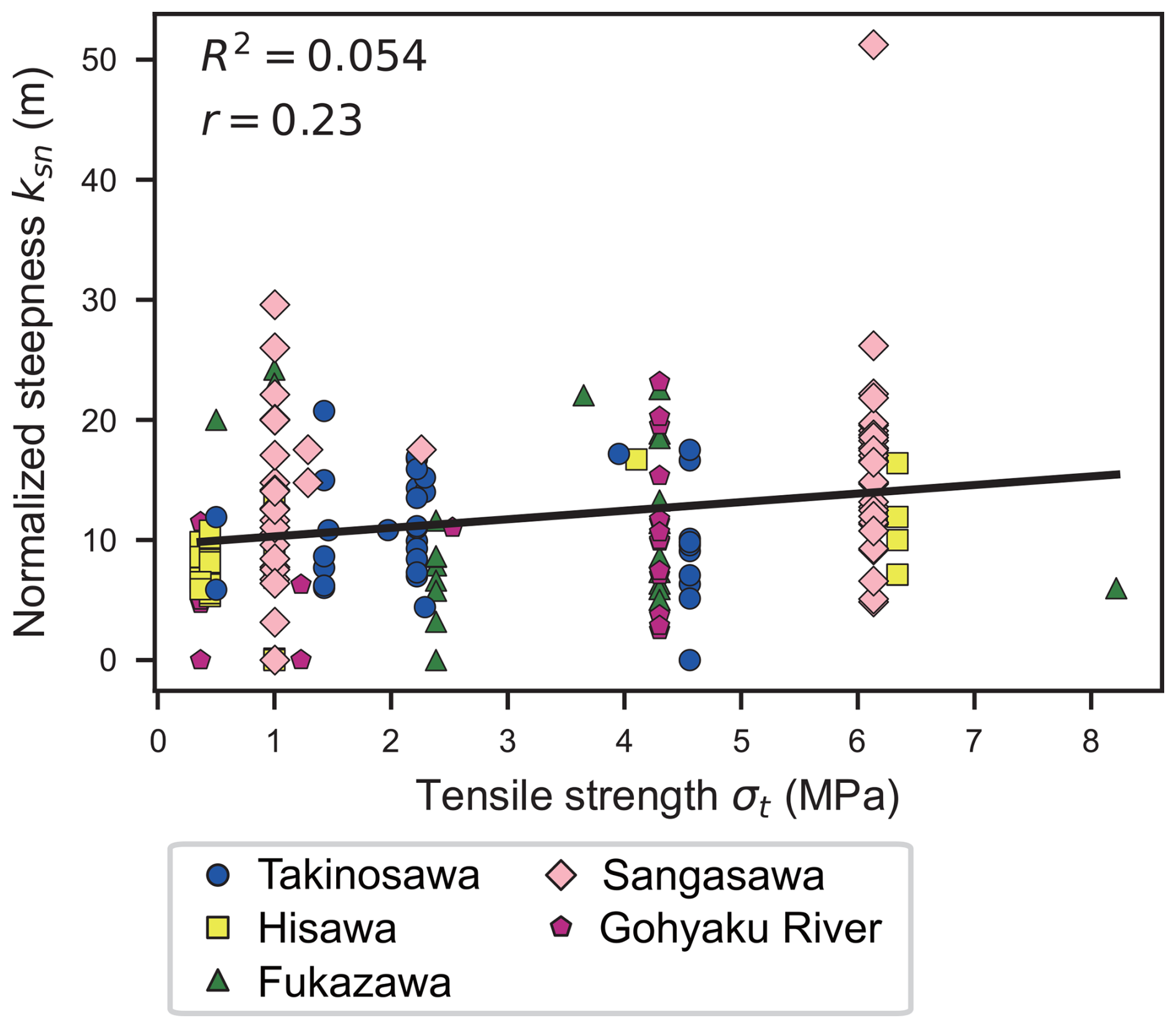
Figure 6 The relationship between normalized steepness and bedrock tensile strengths. Rock tensile strength is weakly correlated with the river steepness.

There are also knickpoints that do not correspond to lithologic boundaries. The knickpoint in the middle Sangasawa corresponds to a significant change in the drainage area of the river. The lithologic boundary between the granodiorite and sandstone is located about 120 m downstream of this knickpoint. The knickpoint downstream of Hisawa coincides with the location of the check dam. In Sangasawa, a check dam is located 10 m downstream of the confluence, whereas the step observed in the topography within the granite occurs upstream of the dam. Several knickpoints are located within the same lithology, such as gneiss in the Fukazawa and Gohyaku rivers, even where no significant change in drainage area or check dam is observed.

The chi-plot results (Fig. 5) did not show knickpoints that correspond to all tributaries. The Takinosawa River has a knickpoint that is absent in other tributaries. The steepness of Takinosawa, Hisawa, and Gohyaku River over χ=20 000 was almost the same; on the other hand, that of Fukazawa and Sangasawa was much steeper.

5.2 Bedrock strengths

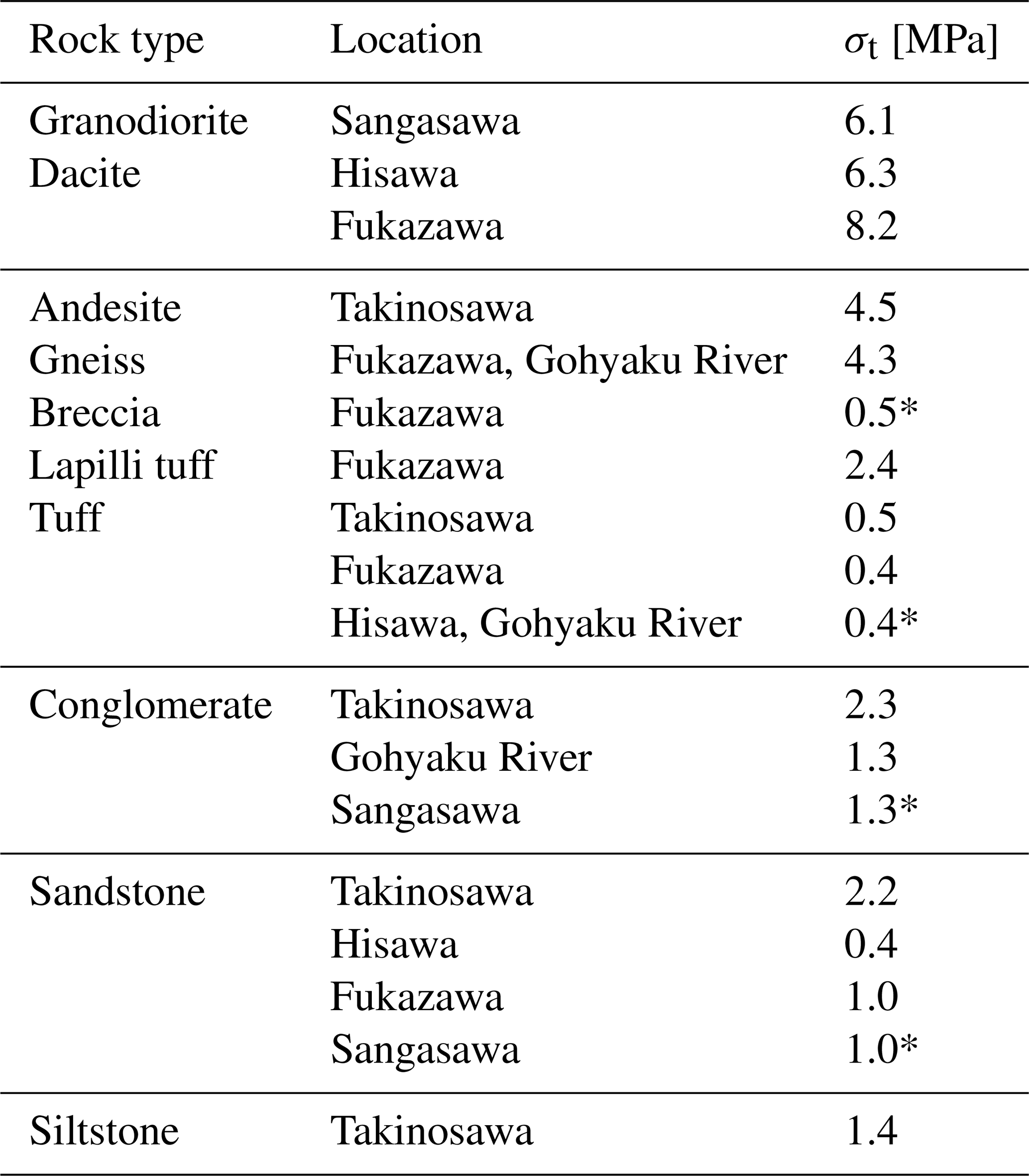
The measured results of the bedrock strengths indicated that igneous and metamorphic rocks exhibited significantly larger tensile strength than sedimentary rocks (Fig. 3; Table 3). The strengths of igneous and metamorphic rocks ranged from 4.3 to 8.2 MPa. Strength measurements accomplished on the dacite at Fukazawa yielded a maximum value of 8.2 MPa, which was more than 18 times larger than the minimum tensile strength of tuffs (0.46 MPa). The sedimentary rocks ranged in tensile strength from 0.4 to 2.4 MPa. They demonstrate variation in their strength depending on the location. The sandstones along Takinosawa were harder than those along Sangasawa.

The relationship between channel slope and bedrock tensile strength exhibited a weak correlation, with a correlation coefficient r of 0.23 and an R² value of 0.054 (Fig. 6). The p-value was 0.0025, indicating that the correlation is statistically significant at the level of α=0.05.

Table 3 Values of rock tensile strength σ_t measured in this study. The asterisk mark (∗) indicates that the tensile strength values were not measured at the tributary, and the values were substituted by those measured in other tributaries.

5.3 Grain size distribution along river channels

5.3.1 Comparison between automated and manual measurements

The median grain size of riverbed gravels automatically measured by the G3Point matched well with manual measurements (Fig. 7). The median grain size was 0.21 m for automated measurements and 0.19 m for manual measurements in the Gohyaku River. Similarly, in the Sakura River, these values were 0.18 and 0.17 m, respectively. Generally, the G3Point program accurately estimates the length of the b-axis. For the a-axis length, the cumulative curves of automated and manual measurements were similar in the regions below the 50th percentile. However, they diverge in the regions where larger grains occur, indicating that the automated measurements are generally accurate except for larger cobbles and boulders. The automated measurements erroneously overestimate the c-axis of gravels (Fig. 7b, d). Nevertheless, the median grain size measured by the fitting of ellipsoids using G3Point differed by only ∼0.02 m from the manual measurement results.

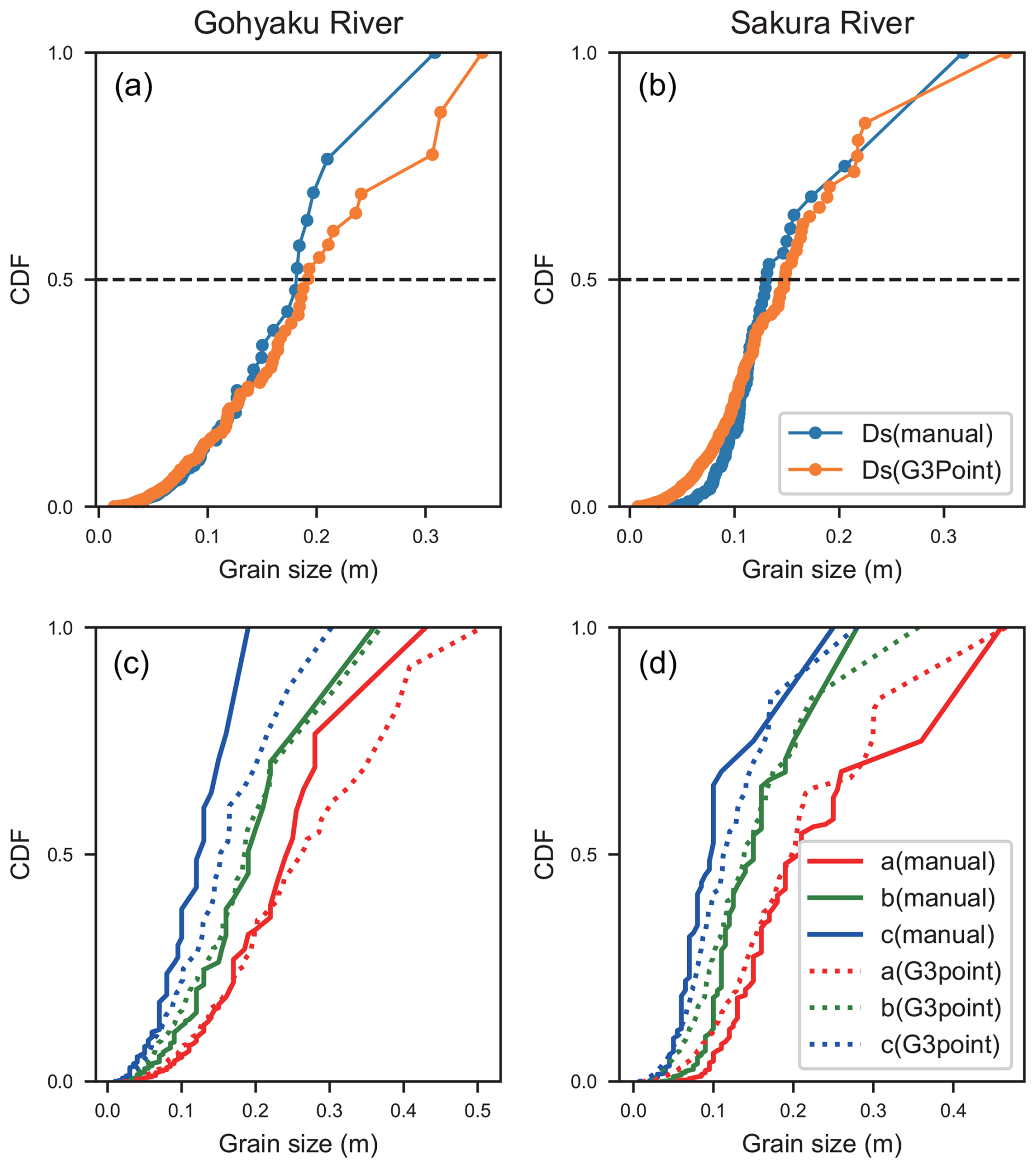
Figure 7 Comparison between automated (G3Point) and manual grain size measurements. The curves represent cumulative distribution functions (CDF), with the vertical axis indicating cumulative volume (%). (a), (b) Orange plots show grain size data obtained using G3Point, while blue plots represent manually measured data. The dashed line indicates the median grain size (D₅₀). The D₅₀ value derived from G3Point was slightly larger than that from manual measurements, with a difference of approximately 0.02 m. (c), (d) Solid lines represent CDFs of the three axes measured manually, whereas dotted lines represent the CDFs of the three axes measured using G3Point.

5.3.2 Grain size distribution

Spatial distributions of grain size along river channels were examined from the D₅₀ values obtained in measured points (Fig. 8). The median grain diameters of riverbed gravels in the study area ranged from 0.4 to 0.7 m. This value is reasonable in the field because the estimated minimum flow depths using ${\mathit{\tau }}^{\ast }=\frac{hS}{R_{\mathrm{b}}{D}_{\mathrm{s}}}$ range from 0.5–1.0 m across the study tributaries under ${\mathit{\tau }}^{\ast }=\mathrm{0.05}$ and R_b=1.65, and these depths are plausible during high-flow events that dominate bedrock erosion.

Fukazawa and Takinosawa exhibited a downstream fining trend, although the spatial variation of grain sizes in Takinosawa was much weaker than in Fukazawa. Other tributaries (Hisawa, Sangasawa, Gohyaku River) exhibited constant grain distributions, and thus the change rate α_d in the grain size trend (Eq. 33) was almost zero. As the median grain diameter decreases, the grain size variation also tends to decrease. In general, grain distribution becomes discontinuous at the point of the check dam, but these grain distribution results did not reflect the effects of the dams for simplicity.

Figure 8 Measured results of grain size distributions for each tributary. (a)–(e) Blue box plots represent the median and quantile ranges of the grain diameter. The red line represents the estimated spatial distribution of D₅₀.

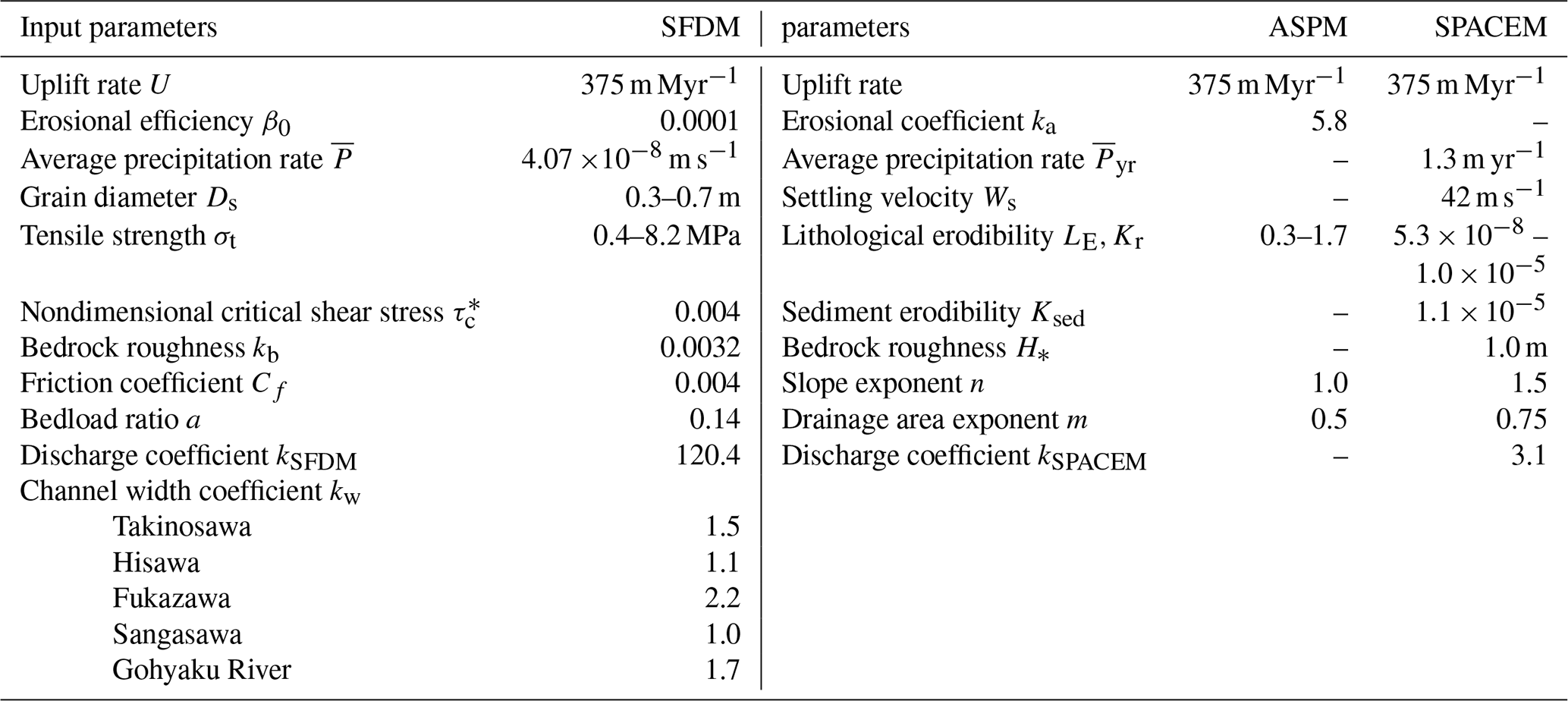
Table 4 Input parameters of the sediment-flux-dependent model.

See each value of D_s and σ_t in Fig. 8 and Tab. 3.

5.4 Model predictions for bedrock river profiles

The numerical experiments using the sediment-flux-dependent model reproduced well the actual river profiles (Fig. 9, red line). The channel width coefficient k_w, which was optimized for the calculation, ranged from 1.0 to 2.2, and the optimized value for the discharge coefficient k_SFDM was 120.4.

Bankfull widths predicted using Eq. (19) with the optimized values of k_w and k_SFDM are consistent with field observations and with estimates derived from 3D point-cloud datasets of the riverbeds. For Takinosawa, the predicted bankfull width is approximately 5–9 m, whereas the observed width is about 7 m. Similarly, the predicted widths for Hisawa and the Gohyaku River are approximately 5–7 and 22–24 m, respectively, which are comparable to the observed widths of about 10 and 15–20 m. For Fukazawa and Sangasawa, the predicted bankfull widths are approximately 13–16 and 4–9 m, respectively. Direct measurements of bankfull width were not available for these rivers.

Both the observed and modeled river profiles exhibited consistently smooth longitudinal trends, regardless of underlying bedrock strength (Fig. 9). The mean squared error between the SFDM and actual profile was 3.5 m, which was the best among the three models (SFDM, ASPM, and SPACEM) examined in this study.

The SFDM prediction for Sangasawa reproduced the knickpoint due to the remarkable change in drainage area. Takinosawa has a concave-upward profile, and the model simulated a similar profile due to the downstream fining grain size distribution. However, the model failed to reconstruct the step-like knickpoints of the river profile observed in Fukazawa and Gohyaku Rivers. This discrepancy was particularly pronounced in areas underlain by hard bedrocks such as granodiorite and gneiss.

Thus, although the SFDM did not capture the fine topographical changes on a scale of a few hundred meters, it accurately reproduced the overall characteristics of the bedrock river profiles.

Figure 9 Results of reproduction of river longitudinal profiles using ASPM, SPACEM, and SFDM. These models were calculated on a 10-m interval grid under the condition that the erosion and the uplift rates are balanced (steady state). (a)–(e) Red line represent the steady-state model profile of SFDM. The colored plots represent the actual river profiles and lithologies. The dash-dot line represents the steady-state profile calculated by ASPM, and the red dot line represents that by SPACEM. The grey line represents drainage area.

In contrast to the SDFM, the profiles predicted by the stream power models (ASPM and SPACEM) did not agree with the actual profiles. Their predictions clearly reflected the controls of variations in bedrock strength through the slope profiles (Fig. 9, red dashed-dot pattern and dashed line). The optimized erosional coefficient for ASPM k_a was 5.8 [yr⁻¹], and the optimized discharge coefficient k_SPACEM for SPACEM was 3.1. The ASPM profile exhibited a remarkable change in slope at the lithologic boundary of the river bedrock types. Especially in Sangasawa, where the contrast in bedrock strength was most pronounced, the ASPM predicted that upstream steepness in granodiorite was 9 times greater than the downstream steepness in sandstone. The actual Sangasawa slope change was very small, so that this ASPM result was significantly different from the actual profile (Fig. 9).

The profiles predicted by the SPACEM still deviated from the actual profiles (Fig. 9), although they were smoother than those of the ASPM. In Sangasawa, the modeled slope of SPACEM changed at the lithological boundary, with the upstream slope being about four times steeper than the downstream slope. The mean squared error between the ASPM and the actual profiles was 21.7, and that of the SPACEM was 13.2.

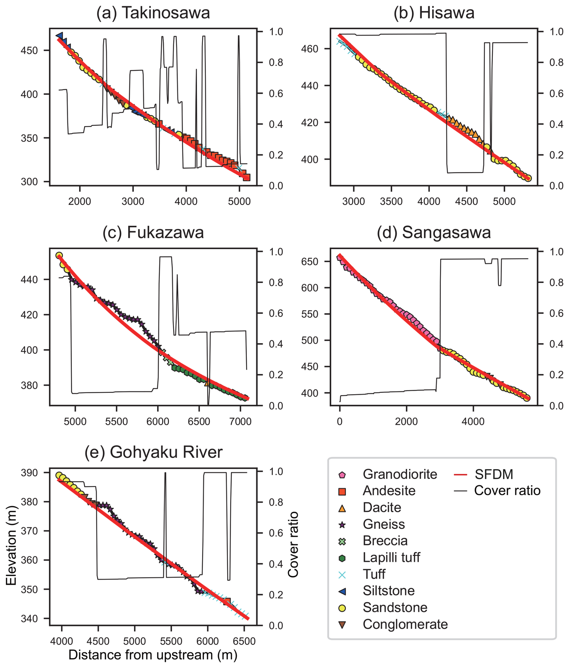
Figure 10 Cover ratio results of the calculations by Eq. (12), with SFDM results. (a)–(e) Black line represents the cover ratio at each site. The cover ratio shows a clear correspondence with lithology.

The results of sensitivity analysis exhibited that in the SFDM, variations in the nondimensional critical shear stress, friction coefficient, and bedload ratio have only minor effects on river profiles, whereas changes in erosional efficiency produce slight gradient variations associated with lithological contrasts but overall stable results (Figs. S1–S8). In contrast, the ASPM exhibited strong parameter sensitivity: river profiles deviate markedly from observations when the slope exponent n exceeds 1.5 or when the drainage area exponent m is below 0.5, indicating that the adopted values (n=1.0, m=0.5) lie within a stable range (Figs. S9–S12). In the SPACEM, channel gradients were less sensitive to n than in the ASPM and remained stable for n≥0.7, while variations in sediment erodibility K_sed within reported ranges caused only minor changes in gradients and RMS (Figs. S13–S18). Overall, the sensitivity analysis confirms that the parameter values used in this study fall within stable regimes and yield results consistent with the observed topography.

6 Discussion

6.1 Why bedrock strength has little influence on local slopes in river longitudinal profile

The field measurements in this study indicated that the bedrock strength has a limited influence on the river longitudinal profiles. Hayakawa and Oguchi (2009), Brocard et al. (2015), and Takahashi (2025) also suggested that the influence of lithological erodibility on the river profile was small. The measurement of bedrock tensile strength included in the present analysis serves to justify this observation.

The numerical experiments imply that the smoothness of the longitudinal profiles of these rivers, in which clear breaks corresponding to a change in lithology are not seen, is attained by the sediment-cover effect (Fig. 11). The sediment-flux-dependent model predicted that the sediment cover ratio mitigated the effect of bedrock strength. Through the cover ratio being higher in soft rocks and lower in hard rocks, erosion is suppressed in soft rock areas, and erosion is promoted in hard rock areas (Fig. 10). Equation (21) indicates that the bedrock strength appears only in the denominator of the first term on the right-hand side of the equation. However, in this equation, the product of the square root of hydraulic roughness $k_{\mathrm{s}}^{\mathrm{1}/\mathrm{2}}$, the squared rock tensile strength ${\mathit{\sigma }}_{\mathrm{t}}^{\mathrm{2}}$, and the uplift rate U (375 m Myr⁻¹ in this study) has a value in the range the order of 10⁻¹¹ to 10⁻¹³ [kg² m${}^{-\mathrm{1}/\mathrm{2}}$ s⁻⁵], while the term of the product of coefficient β₀, the grain size $D_{\mathrm{s}}^{\mathrm{1}/\mathrm{2}}$, and sediment supply rate q_s is the order of 10⁻¹⁰ [kg² m${}^{-\mathrm{1}/\mathrm{2}}$ s⁻⁵]. Thus, it is clear from the equation that the value of rock tensile strength has little effect on the resulting slope. The mechanical explanation for controlling the sediment cover ratio in relation to lithology is as follows.

Considering the cover ratio, even minor changes in river slope can substantially alter erosion rates, effectively mitigating the influence of the bedrock strength. The sediment cover ratio on the bedrock surface increases as the sediment transport capacity approaches the actual sediment supply. Conversely, the cover ratio P_c decreases when the sediment supply is limited or when transport capacity increases. This dynamics is explicitly considered in the sediment-flux-dependent model, in which P_c is formulated as the ratio of sediment supply q_s to the transport capacity q_t (Sklar and Dietrich, 2004; Chatanantavet and Parker, 2009). Here, the sediment supply is primarily governed by upstream conditions, while the transport capacity q_t is controlled by the bed shear stress, which increases with the channel slope S. Therefore, under constant sediment supply, the cover ratio P_c is slope-dependent (Fig. 11). This dependence is particularly pronounced at low gradients, where the bed shear stress is near the threshold for the gravel mobilization, making P_c highly sensitive to small changes in slope (Fig. 12). Because the sediment cover shields the bedrock from direct impact by bedload particles, even slight variations in slope – and thus in cover ratio – can lead to significant differences in erosion rates (Fig. 10).

As a result, river longitudinal profiles tend not to exhibit marked changes across lithologic boundaries unless the slope becomes exceptionally steep. Although channel gradients over resistant lithologies are marginally steeper than those over weaker ones, the difference is often too subtle to be discerned either in numerical simulations or natural river profiles (Figs. 6, 9, and 11). Korup and Schlunegger (2009) reported that the slope can vary by as much as 0.08 depending on lithology in hillslope areas. In comparison with their results, such abrupt lithology-driven slope changes do not occur in the alluvial-bedrock reaches investigated here.

This finding aligns with previous studies. Sklar and Dietrich (2006) demonstrated that the rock strength exerts only a limited influence on channel profiles in models that incorporate the sediment cover effect. Similarly, Guryan et al. (2024) showed that the variability in channel slope due to differences in rock erodibility is smoothed out when sediment cover dynamics are included in numerical simulations. The present study further supports these findings by demonstrating, through numerical experiments using field-derived datasets, that sediment cover effectively offsets the influence of bedrock strength on river profile morphology.

This study proposes that the relationship between the cover ratio and river slope is a critical factor, and the SFDM well reproduces this relationship. The ASPM does not consider the sediment cover ratio, and therefore, it fails to predict the actual river longitudinal profiles. While the SPACEM (Guryan et al., 2024) also considers the cover ratio, its reproducibility is inferior to that of the SFDM (Fig. 9). The reason for this discrepancy lies in the formulation of the relationship between cover ratio P_c and channel slope S in the SPACEM. Figure 12a, b illustrates cover ratio and erosional rates against slopes for both SPACEM and SFDM. Both models assume that the erosional rate is proportional to the ratio of bedrock exposure. In the case of SFDM, the bedrock exposure ratio is defined as 1−P_c. In contrast, SPACEM adopts the log-scale definition $e^{-H/H_{\ast }}$, resulting in a weaker topographic response to variations in the ratio of sediment cover. At present, the former formulation is more suitable for representing actual river profiles. However, there is no physical basis to suggest that the cover ratio is linearly correlated with the sediment supply/transport capacity ratio; therefore, further investigation is necessary to improve the cover (or exposure) ratio to better fit real-world conditions in future research.

It should be noted that several small-scale knickpoints are present in the rivers of the study area (Fig. 5) that cannot be explained by any of the models considered in this study. Most of these knickpoints occur independently of bedrock strength, and some display trends opposite to those expected from bedrock strength, such as occurring in relatively hard rock reaches with gentle channel gradients (Fig. 4). All models used in this study assume that rivers are in a steady-state balance between rock uplift and erosion. The presence of these minor knickpoints therefore suggests that parts of the river profiles may locally deviate from equilibrium. Knickpoints generated by the processes, such as past sea-level fluctuations or localized fault activity in bedrock rivers, are known to migrate upstream over time and eventually dissipate in upstream reaches (Whipple and Tucker, 1999). Such transient processes are not represented in equilibrium-based models. Despite these limitations, the models employed here – particularly the SFDM – successfully reproduce the overall longitudinal profile characteristics of the rivers. This indicates that, at a macroscopic scale, the river systems in the study area can reasonably be regarded as being close to equilibrium.

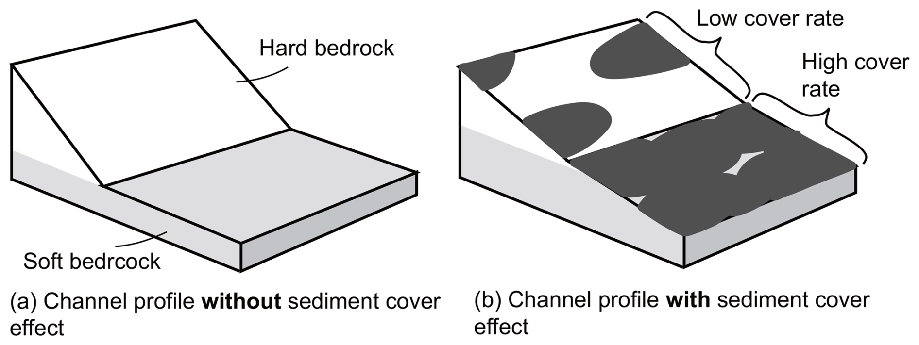
Figure 11 Comparison of channel profiles across two lithologies with and without sediment cover. (a) Without sediment cover. (b) With sediment cover.

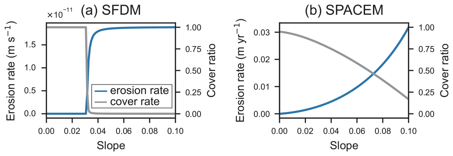
Figure 12 Changes in erosion rate and sediment cover ratio with slope in SFDM and SPACEM. The blue line represents changes in erosion rate, while the gray line indicates changes in sediment cover ratio. (a) SFDM result. Erosion rate and cover ratio change rapidly in a specific region of the slope. (b) SPACEM result. Both erosion rate and cover ratio change gently.

6.2 Indirect lithologic controls for river longitudinal profiles

Although bedrock strength may not directly control local channel gradients, lithology can still exert an indirect influence on the entire morphology of channel longitudinal profiles by shaping the grain size distribution and sediment flux as mentioned in Lai et al. (2021). As shown in Eq. (21), the primary factors determining channel profiles are the water discharge per unit width q_w, grain size D_s, and sediment flux q_s. Among these, the latter two parameters are potentially regulated by the lithologic characteristics of the upstream drainage areas.

Grain size and distributions of sediment are known to vary significantly depending on the lithology of their drainage basins (Parker, 1991; Kodama, 1994; Sklar et al., 2017; Roda-Boluda et al., 2018; Verdian et al., 2021; Takahashi, 2025). Sediment grains are initially produced on hillslopes through physical and chemical weathering processes, where lithology, along with tectonics and climate, plays a critical role in determining grain sizes (Sklar, 2024). Field measurements have consistently highlighted the importance of lithology, owing to its control on the physical and chemical properties of parent rocks, in influencing grain size distribution. For instance, Sklar et al. (2017) demonstrated a clear correlation between rock strength and the sizes of rock fragments measured in soils in California. Similarly, Verdian et al. (2021) conducted field measurements of clast sizes, indicating that gravels derived from massive granitic plutons exhibited the largest, those from surficial basalt flows had intermediate sizes, and those from marine ribbon chert were the smallest. Since tool size undergoes downstream fining through abrasion, local bedrock lithology alone does not uniquely determine channel gradient. In contrast, basin-integrated lithologic controls can still shape longitudinal profiles through their influence on tool production and size distributions. Collectively, these studies underscore the significant control exerted by hillslope lithology on grain size.

Bedrock lithology in hillslope regions also controls the ratio of bedloads to the eroded materials (Chatanantavet and Parker, 2009), which affects the sediment flux q_s provided to streams. The sediment supply rate depends on the erosional rate, the drainage area, and the mode of mechanical weathering that determines the ratio of bedload materials in sediment (Eq. 17). For example, Roda-Boluda et al. (2018) examined the frequency and size of landslides in southern Italy, focusing on their relationship with the local slope steepness and rock strength. They discovered that the frequency of landslides increases as the slope is composed of softer rock, which promotes the larger sediment production rates.

Thus, the lithologic composition of bedrock across the drainage basin from hillslopes to fluvial zones can play a critical role in determining the overall longitudinal profile of river channels. Supporting this notion, the field-based analysis by Takahashi (2025) in the Tsugaru region of Japan demonstrated that variations in channel morphology are strongly linked to differences in sediment load and grain size, both of which are influenced by upstream lithology. The findings of this study are consistent with this interpretation. The bedrock types in the hillslope regions of the studied tributaries can be broadly divided into two categories: granodiorites and sedimentary rocks. Granodioritic bedrocks are predominantly exposed in the upstream catchments of Fukazawa and Sangasawa, whereas sedimentary rocks dominate the upstream areas of Takinosawa, Hisawa, and Gohyaku River (Kubo et al., 2003; Yamamoto and Sakaguchi, 2023). Chi-plots analysis (Fig. 5) revealed that the channel steepness indices of Fukazawa and Sangasawa tended to be notably higher in their upper reaches compared to the other tributaries.

This pattern suggests that upstream lithology – specifically, the presence of more resistant granodiorite – may enhance channel steepness by influencing sediment grain size and transport rates. These observations underscore the indirect yet significant role of lithologic variation in controlling longitudinal channel profile. Further quantitative predictions of such lithologic controls remain a key challenge for future research.

7 Conclusions

To investigate the influence of bedrock strength on fluvial morphology, this study combined field surveys with numerical experiments. The results revealed that the sediment cover effect plays a key role in mitigating the impact of variations in bedrock erodibility on river profile morphology.

Field surveys were conducted in the Abukuma River basin in northeastern Japan, where tributaries incise bedrock of varying lithologies exposed in close proximity. Bedrock strength and riverbed gravel grain size distributions were measured in each tributary. Tensile strength of bedrock samples, obtained through the Brazilian splitting test, varied by more than an order of magnitude. Despite this, no significant differences were observed in the channel slopes across the longitudinal profiles of these rivers (Fig. 6).

To explain the apparent insensitivity of river longitudinal profiles to local variations in bedrock strength, we carried out numerical experiments using three models that account for bedrock erodibility to different extents: the sediment-flux-dependent model (SFDM), the area-based stream power model (ASPM), and the stream power with alluvium conservation and entrainment model (SPACEM). All three incorporate bedrock erodibility, while SFDM and SPACEM also include the effects of sediment cover. Among them, only SFDM explicitly incorporates the sediment tool effect, which describes the enhanced erosion by mobile sediment particles.

The SFDM simulations demonstrated that the sediment cover effect buffers the influence of rock erodibility on channel slope. In regions with high bedrock erodibility, increased erosion tends to lower channel gradients. This reduction in slope, in turn, reduces sediment transport capacity, leading to greater sediment cover. The increased cover inhibits further erosion by reducing the sediment tool effect, establishing a negative feedback loop. This mechanism effectively dampens variations in slope, even in the presence of substantial differences in bedrock strength.

The numerical results emphasize the importance of incorporating both sediment cover and the sediment tool effect when evaluating the geomorphic consequences of bedrock erodibility. Among the three models, SFDM most accurately reproduced the observed longitudinal river profiles, exhibiting little to no slope variation in areas of differing lithology. In contrast, ASPM, which does not consider sediment cover, predicted prominent slope breaks inconsistent with field observations. SPACEM performed better by including sediment cover, but still exhibited unrealistic local slope variations, as it lacks explicit treatment of the sediment tool effect.

While bedrock strength does not directly control local channel gradients, this study suggests that upstream lithology can indirectly influence overall channel steepness by modifying sediment grain size and supply rates. Future research should aim to incorporate more extensive datasets on gravel characteristics to better quantify this indirect relationship between bedrock properties and fluvial morphology.

Appendix A: Notation

a	the ratio of the bedload to the total sediment supply
A	drainage area (m2)
A0	a reference drainage area (m2)
Cf	a friction coefficient
D	a diameter of the specimen (m)
Ds	grain diameter (m)
E	erosion rate (m s−1)
Eeq	erosion rate in steady state (m s−1)
Er	erosion rate in SPACEM (m yr−1)
Es	rate of entraintment in SPACEM (m yr−1)
g	acceleration of gravity (m s−2)
H	thickness of sediment cover (m)
H∗	bedrock roughness scale (m)
Ir	rate of particle impacts per unit area per unit time
kSFDM	discharge coefficient in SFDM
kSPACEM	discharge coefficient in SPACEM
ka	erosional coefficient (L1−2 m T−1)
ks	hydraulic roughness height (m)
ksn	normalized steepness
kv	rock resistance coefficient
kw	channel width coefficient
Kr	bedrock erodibility (L1−2 m T−1)
Kr,i	the ith rock type erodibility
Ksed	sediment erodibility
L	length of the specimen (m)
LE	relative lithological erodibility index
Ls	saltation hop length (m)
m	a drainage area exponent in stream power models
Mp	particle mass (kg)
n	a slope exponent in stream power models
$\stackrel{\mathrm{‾}}{P}$	average precipitation rate (m2 s−1)
${\stackrel{\mathrm{‾}}{P}}_{\mathrm{yr}}$	mean annual precipitation rate (m2 yr−1)
Pc	cover ratio
Pmax	maximum load (kN)
q	water discharge per unit width (m2 s−1
qs	sediment flux volume per unit width (m2 s−1)
qt	sediment transport capacity per unit width (m2 s−1)
qw	water discharge per unit width (m2 s−1)
qw,yr	mean annual water discharge per unit width (m2 yr−1)
Qw	water discharge (m3 s−1)
Qw,yr	mean annual water discharge (m3 yr−1)
r	a correlation coefficient
Rb	nondimensional buoyant density of sediment
S	channel slope
U	uplift rate (m s−1)
Ui	particle impacr velocity (m s−1)
Vi	average volume eroded per particle impact
wsi	vertical sediment velocity on impact (m s−1)
W	channel width (m)
Ws	settling velocity (m s−1)
x	distance along the channel from upstream (m)
Y	Young's modulus (MPa)
α	saltation impact angle
αd	change rate of the grain diameter
β0	an empirical erosional coefficient
εv	unit volume detachment energy (J m−3)

η	bedrock elevation (m)
θ	channel concavity index
κa	roughness coefficient linear to the grain size (m)
κb	bedrock roughness (m)
ρs	sediment density (kg m−3)
ρw	water density (kg m−3)
σt	bedrock tensile strength (MPa)
σt,i	tensile strengths of the ith rock type (MPa)
σt,tuff	tensile strength of tuff (MPa)
τb	bed shear stress (Pa)
τ∗	nondimensional bed shear stress
${\mathit{\tau }}_{\mathrm{c}}^{\ast }$	nondimentional critical shear stress
ϕ	sediment porocity