the Creative Commons Attribution 4.0 License.
the Creative Commons Attribution 4.0 License.
 | 27 Jun 2018
Characterizing the complexity of microseismic signals at slow-moving clay-rich debris slides: the Super-Sauze (southeastern France) and Pechgraben (Upper Austria) case studies
Naomi Vouillamoz
Sabrina Rothmund
Manfred Joswig
Soil and debris slides are prone to rapid and dramatic reactivation. Deformation within the instability is accommodated by sliding, whereby weak seismic energies are released through material deformation. Thus, passive microseismic monitoring provides information that relates to the slope dynamics. In this study, passive microseismic data acquired at Super-Sauze (southeastern France) and Pechgraben (Upper Austria) slow-moving clay-rich debris slides (“clayey landslides”) are investigated. Observations are benchmarked against previous similar case studies to provide a comprehensive and homogenized typology of microseismic signals at clayey landslides. A thorough knowledge of the various microseismic signals generated by slope deformation is crucial for the future development of automatic detection systems to be implemented in landslide early-warning systems. Detected signals range from short-duration (< 2 s) quake-like signals to a wide variety of longer-duration tremor-like radiations (> 2 s – several min). The complexity of seismic velocity structures, the low quantity and low quality of available signal onsets and non-optimal seismic network geometry severely impedes the source location procedure; thus, rendering source processes characterization challenging. Therefore, we constrain sources' locations using the prominent waveform amplitude attenuation pattern characteristic of near-source area (< about 50 m) landslide-induced microseismic events. A local magnitude scale for clayey landslides (ML−LS) is empirically calibrated using calibration shots and hammer blow data. The derived ML−LS returns daily landslide-induced microseismicity rates that positively correlate with higher average daily displacement rates. However, high temporal and spatial resolution analyses of the landslide dynamics and hydrology are required to better decipher the potential relations linking landslide-induced microseismic signals to landslide deformation.
- Article
(16793 KB) - Full-text XML
- BibTeX
- EndNote


Slow-moving soil and debris slides developed in tectonized marl formations are characterized by seasonal dynamics as well as by sudden (generally rainfall triggered) reactivation and liquefaction phases (Malet et al., 2005; Hungr et al., 2014). The slow deformation of soil and debris slides is expected to generate elastic accumulation and rupture, which releases seismic energy within the landslide body. Therefore, passive seismic monitoring is a good approach to monitor and mitigate slope instabilities, as it provides high temporal resolution data (sample rates up to 1000 Hz) in near real-time that relate to the dynamics of the landslide. This means that the transition (and rapid transformation) of the landslide from steady-state sliding into a debris flow may be detected and slope failure anticipated.
Seismic investigations of natural and artificial slope instabilities started in the 1960's with acoustic emission (10–1000 kHz) (e.g., Beard, 1961; Cadman and Goodman, 1967; Jurich and Miller Russell, 1987) and have been complemented during the last decades by an increasing number of passive microseismic monitoring studies (1–1000 Hz), carried out in various geological contexts. The shear boundaries of the Slumgullion earthflow in Colorado were first investigated by Gomberg et al. (1995) as a strike-slip fault zone analog. The study confirmed the existence of detectable brittle deformation processes associated with slide deformation. In Europe, clayey landslides investigated include the Heumoes slope in the Austrian Vorarlberg Alps (Walter and Joswig, 2008; Walter et al., 2011), the Super-Sauze landslide in the southwest of the French Alps (Walter and Joswig, 2009; Walter et al., 2012; Tonnellier et al., 2013; Provost et al., 2017) and the Valoria landslide in the northern Apennines in Italy (Tonnellier et al., 2013). Examples of case studies carried out at rockslides include, but are not limited to, the following: the Randa rockslide in the Swiss Alps (Eberhardt et al., 2004; Spillmann et al., 2007); the Åknes rockslide in Norway (Roth et al., 2005; Fischer et al., 2014); the Séchilienne rockslide in the southeastern French Alps (Helmstetter and Garambois, 2010; Lacroix and Helmstetter, 2011); and the Gradenbach, Hochmais-Atemskopf and Niedergallmigg-Matekopf deep-seated rock slope deformations in the eastern Austrian Alps (Brückl and Mertl, 2006; Mertl and Brückl, 2007; Brückl et al., 2013).
Observed near microseismic signals (source–receiver distances < 500–1000 m) comprise microearthquake events, for which Gomberg et al. (1995) introduced the term “slidequake”. Such events have been reported both at rock and debris slides and are inferred to be associated with fracture processes in the host rock, at the sliding surface or within the landslide body. Rockfall and rock-avalanche signals were also characterized at steep debris slides and at rock slides (Helmstetter and Garambois, 2010; Walter et al., 2012; Tonnellier et al., 2013; Provost et al., 2017). In addition, a wide variety of tremor signals have been reported marginally (Gomberg et al., 1995; Brückl and Mertl, 2006; Mertl and Brückl, 2007; Spillmann et al., 2007; Gomberg et al., 2011; Walter et al., 2012; Tonnellier et al., 2013; Provost et al., 2017). No common typology has yet been suggested for these signals and the signal source interpretation remains speculative.
This study aims at proposing a classification of microseismic signal types as recorded by tripartite microseismic arrays deployed at slow-moving clay-rich debris slides (“clayey landslides”). Tripartite microseismic arrays are suited for the determination of the back azimuth and apparent velocity of an incoming signal; hence, they provide key information about the signal source location (e.g., Joswig, 2008; Sick et al., 2012; Vouillamoz et al., 2016). The classification of microseismic signals is based on the waveform and spectral attributes of the signals and uses microseismic observations reported by similar case studies as a benchmark. Because of the lack of clear phase arrivals and signal coherence across the seismic network at clayey landslides, standard seismological approaches to establishing the source location using arrival times derive minimum uncertainties of ±50 m for near-source area microseismic events (e.g., Tonnellier et al., 2013). Therefore, we apply an alternative method based on seismogram amplitude information to constrain the source–receiver distance of near-source area landslide-induced microseismic events. The technique is generally referred in the literature as amplitude source location (ASL) and has been used following various approaches to locate microseismic sources recorded at distances of less than a few kilometers at volcanoes (e.g., Jolly et al., 2002; Battaglia, 2003; Battaglia et al., 2005) or glaciers (e.g., Jones et al., 2013; Röösli et al., 2014), as well as for different kinds of mass motion, including lahars (e.g., Kumagai et al., 2009) and debris flows (e.g., Walter et al., 2017). We applied a simple ASL approach in which calibration shots and hammer blows carried out in the study area were used to empirically evaluate amplitude attenuation patterns. Then, with the aim of reducing bias and errors in the estimation of landslide-induced microseismicity rates, the distance attenuation function of the local magnitude scale was calibrated for clayey landslides using the active microseismic datasets. Detected microseismic events were finally gathered in a comprehensive catalog. The final catalog of landslide-induced microseismic signals provides an important basis for a multidisciplinary comparative analysis with other landslide observations (such as displacement, cracks and fissures development) or with hydrometeorological data to gain knowledge about landslide dynamics; the catalogue also presents an initial signals library to train automatic detection and classifier systems.
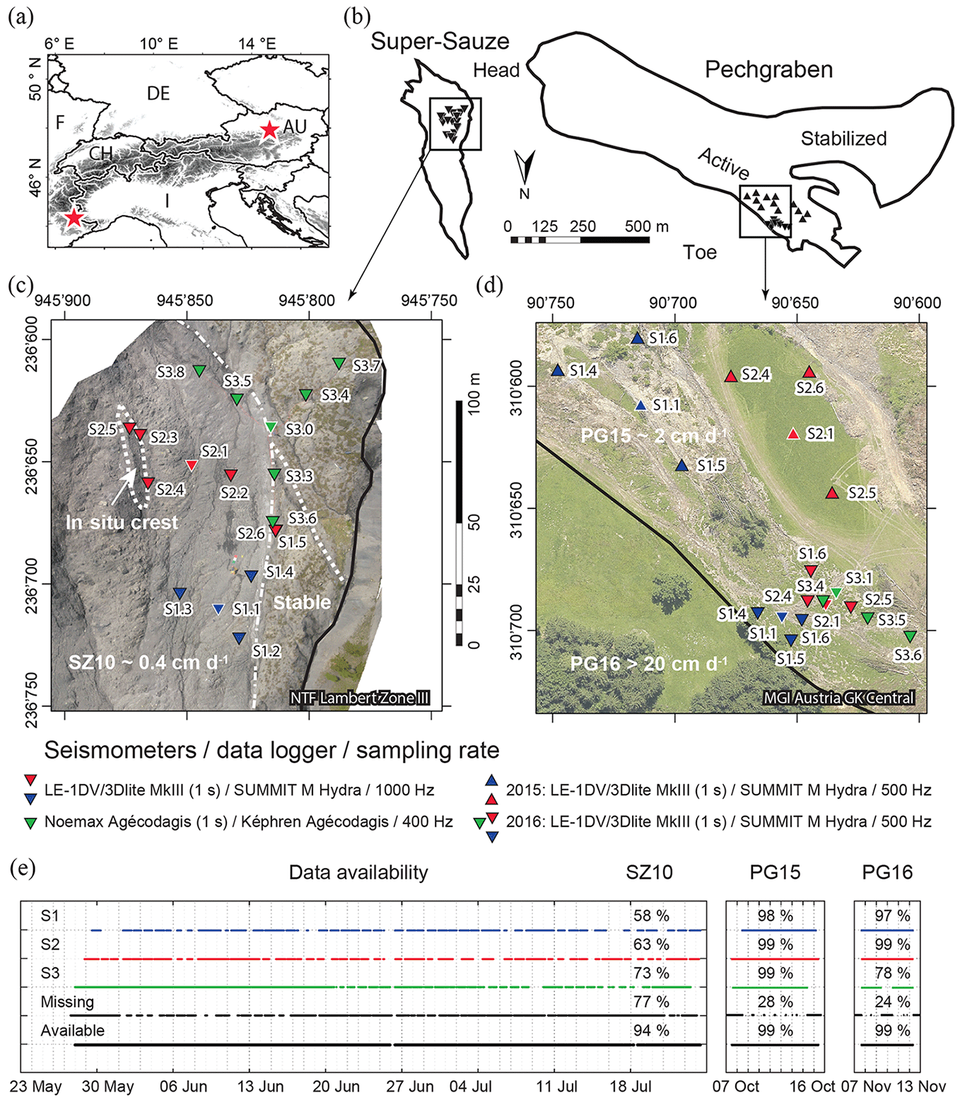
Figure 1Data overview. (a) Location of Super-Sauze (southeastern France) and Pechgraben (Upper Austria) clayey landslides (stars). (b) Orthogonal projection of Super-Sauze and Pechgraben instabilities including locations of instrumented areas during the three field campaigns SZ10, PG15 and PG16. (c–d) Zoom in of Super-Sauze and Pechgraben seismic networks, where triangles indicate the seismic stations and colors refer to different tripartite arrays (S1, blue; S2, red; and S3, green). The average daily displacement rates prevailing during individual field campaigns are indicated; white dashed lines indicate main subparts of the landslide and black bold lines show the limits of the landslides. 3-C seismometers (S1.1, S2.1, S3.0 and S3.1) are highlighted by white outlines. Orthophotos credits: Super-Sauze, Rothmund et al. (2017); Pechgraben, Lindner et al. (2014, 2016). (e) Data record availability for individual seismic arrays based on 2 min data segments. The “missing” line indicates incomplete records (measurements from one or two arrays are missing); the “available” line shows where at least one array is recording.
Seismic measurements were acquired at two well-instrumented slopes: the Super-Sauze (southwestern French Alps) and Pechgraben (Upper Austria) landslides (Fig. 1a–b). Both instabilities are characterized by a clay-rich matrix transporting rigid boulders of marls and limestone (including the remains of vegetation at Pechgraben) with moving rates ranging from a few millimeters to several tens of centimeters per day in the investigated areas and periods (Fig. 1c–d). In the monitored areas, the thickness of the instability reaches more than 10 m at Super-Sauze, but does not exceed a few meters (2–4 m) at Pechgraben. More details about the two landslides can be found in Malet (2003), Travelletti (2011) and Tonnellier et al. (2013) for Super-Sauze, and Lindner et al. (2014) and Lindner et al. (2016) for Pechgraben.
Continuous data from the three following seismic campaigns were investigated (Fig. 1):
-
Super-Sauze 2010 (SZ10): 28 May–24 July 2010; 58 days; 18 sensors over 2 ha; average displacement of 0.4 cm d−1, obtained by daily dGNSS (differential global navigation satellite system) measurements.
-
Pechgraben 2015 (PG15): 7–15 October 2015; 9 days; 12 sensors over 6 ha; average displacement of 2 cm d−1, obtained by weekly dGNSS measurements.
-
Pechgraben 2016 (PG16): 8–12 November 2016; 5 days; 12 sensors over 1 ha; average displacement of more than 20 cm d−1, estimated by triangulation, using grids of fixed nails (both on the stable and active parts of the slide) in addition to daily photo-monitoring.
Tripartite seismic arrays were deployed with station spacing of 5–50 m (Fig. 1c–d). Each seismic array consists of a central three-component (3-C) short-period seismometer (Lennartz 3Dlite) which is surrounded by three to six vertical short-period seismometers (Lennartz 1Dlite). The seismometers were buried about 30 cm deep in the landslide material. Data were collected by battery powered SUMMIT M Hydra data loggers. At Super-Sauze, the array S3 consists of Noemax Agécodagis velocimeters (one 3-C and six verticals) with an associated band-pass of 0.1–80 Hz, connected to a Képhren Agécodagis acquisition system powered by solar panels. This array is part of a permanent monitoring installation (RESIF, 2006). Therefore, the seismometers feature a robust installation and are housed in plastic drums on top of a concrete slab. A comparison of the data collected by the different installation systems proved them to be consistent: identical waveforms featuring similar amplitudes are observed for microseismic events recorded at the co-located stations S1.5, S2.6 and S3.6; local, distant and teleseisms are recorded with similar amplitudes across the complete seismic network. No significant difference in terms of waveform scattering was found for signals recorded by stations installed in the more stable areas. At Pechgraben, due to the relatively large aperture (30–50 m) of the seismic arrays in the PG15 campaign, many near-source area microseismic events were recorded by less than three sensors. Consequently, a denser seismic network configuration was designed for the PG16 campaign. Inherent difficulties of operating systems continuously on landslides resulted in partially incomplete datasets (Fig. 1e). This aspect must be considered when evaluating the completeness of landslide-induced microseismic catalogs.
Data were analyzed following the “Nanoseismic Monitoring” methodology using the NanoseismicSuite software package developed at the Institute for Geophysics of the University of Stuttgart (Wust-Bloch and Joswig, 2006; Joswig, 2008; Sick et al., 2012; Vouillamoz et al., 2016). The method is supported by a real-time, analyst-guided interactive multi-parameter visualization approach. First, signals are identified by visual screening of continuous sonograms, where sonograms are logarithmically scaled spectrograms featuring a dynamic frequency-dependent noise adaptation (Joswig, 1990, 1995, 1996). The enhanced visualization of sonograms has the unmatched power to facilitate the detection and recognition of various types of weak signal energies in low-SNR (signal-to-noise ratio) conditions without a priori knowledge (Joswig, 1990; Sick et al., 2012; Vouillamoz, 2015; Vouillamoz et al., 2016; Sick, 2016). The SonoView module of the NanoseismicSuite software provides a dynamic layout, where single-trace sonograms or multi-trace (array-stacked) super-sonograms are visualized on a common timeline, with up to several hours on one laptop screen. Different resampling can be applied to the data, enabling the focus to be directed at various event types (short or long duration, low or high frequency). Detected events are tagged and synchronized in the linked HypoLine module of the software suite for further evaluation. There, waveforms are analyzed interactively to provide an optimized graphical hypocentral solution. Seismograms can be simultaneously processed in network and array mode, taking advantage of the tripartite configuration of the seismic mini-arrays (see Joswig, 2008 and Vouillamoz et al., 2016 for a comprehensive description of the HypoLine software). The strength of the method is its ability to easily detect and successfully evaluate any kind of signals without a priori knowledge in noisy environments. The drawback is that the process is not automated. Consequently, it is time-consuming and not well-suited to large datasets (years). Results may also not be 100 % reproducible.
Much attention was paid to designing a comprehensive database and gathering all microseismic signals observed by passive microseismic monitoring on active debris slides. Continuous sonograms of the three seismic datasets (SZ10, PG15 and PG16) were visually screened in SonoView. To avoid false noise detection, special attention was paid when screening daytime measurements contaminated by anthropogenic noise caused by geophysicists or geotechnical work carried out on the slope. Only signals coherently recorded by at least three sensors were declared as detections. Each detection was first evaluated individually and interactively in HypoLine, where phase information was picked, and time offsets between array-correlated wave packets were used to derive apparent velocity and back azimuth information following the approach described in Fig. 5 of Vouillamoz et al. (2016). Waveform and spectral features of all signals were then analyzed semi-quantitatively using MATLAB® routines as follows:
-
For each event, all vertical trace seismograms of the seismic network were visualized on a common timeline with normalized and non-normalized amplitudes, using a set of pre-defined time windows (5, 10, 30, 60 and 120 s). The signal's coherency, the event duration and the waveform amplitude attenuation pattern across the seismic network were checked.
-
Traces on which the signal of interest is contaminated by noise and traces that did not record the event were tagged and discarded from further analysis.
-
For each trace that recorded the event, the non-logarithmic spectrogram, the unfiltered waveform and a series of waveforms with selected band-pass filters were plotted and evaluated.
-
The amplitude spectrum (FFT, fast Fourier transform) was calculated to estimate the dominant frequency content of the signals. Since the short source–receiver distances of the considered signals do not allow a clear separation of body waves and surface waves, amplitude information was taken as the maximum absolute zero-to-peak amplitude of the signal unfiltered vertical seismogram.
3.1 Classification
Potential landslide-induced microseismic events were finally classified considering the following features:
-
Apparent velocity of trackable wave packets. Well-constrained apparent velocities (computed by array processing for wave packets showing at least four traces with correlation thresholds > 70 %) ranging from less than 0.2 km s−1 to more than 5.0 km s−1. We distinguish two main classes of apparent velocities: < 2.0 km s−1 (top most volume of the landslide body and landslide body) and > 2.0 km s−1 (sedimentary bedrock), in agreement with published velocity profiles of clayey landslides (Williams and Pratt, 1996; Tonnellier et al., 2013).
-
Clustering of events. Single events are distinguished from events featuring multiple jolts and repeated energetic spikes.
-
Signal duration in seconds. Signals are classified in three duration classes: short-duration (< 2 s), medium-duration (2–20 s) and long-duration signals (> 20 s – minutes).
-
Amplitude attenuation pattern. The signals of landslide-induced microseismic sources are expected to be severely attenuated, mainly because of their propagation through heterogenous clay-rich soils of varying water saturation (e.g., Koerner et al., 1981). Calibration shots and hammer blows carried out at Super-Sauze and Pechgraben showed that sources occurring within the seismic network feature prominent waveform attenuation across the seismic network, whereas sources originating a few hundred meters outside the seismic network feature waveforms that are homogeneously attenuated, resulting in similar signal amplitudes across the seismic network. Therefore, only microseismic events featuring prominent and consistent attenuation of the signal maximum amplitudes across the seismic network are considered as a nearby source, potentially induced by the landslide dynamics.
-
Frequency-related characteristics. The distribution of the dominant energies in individual station records is evaluated from the signal spectrogram, from a selection of band-passed filtered waveforms (1–5; 5–20; 20–50; 50–100 and 100–200 Hz) as well as from the amplitude spectrum. Signals with dominant energies mainly below 50 Hz are separated from events featuring dominant energies well above 50 Hz. Additional observed characteristics include harmonic peaks, dispersive, gliding or multiple-band dominant frequencies. These frequency-related characteristics are illustrated in the event classification (Sect. 4).
Based on these features, and using previous studies (Gomberg et al., 1995; Walter and Joswig, 2008, 2009; Gomberg et al., 2011; Walter et al., 2012; Tonnellier et al., 2013; Provost et al., 2017) as a benchmark, microseismic events detected at clayey landslides are gathered in three main groups, which we describe and discuss in Sect. 4:
-
Earthquakes (local, regional and teleseisms).
-
Quakes (source–receiver distance < 50–500 m).
-
Tremors (landslide-induced tremor signals and external sources of tremor-like radiations).
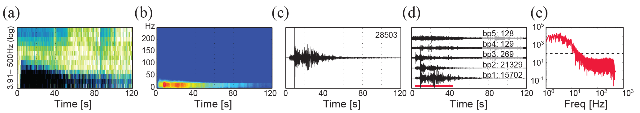
Figure 2Seismic features of an earthquake displayed using different graphical representations. Regional event (110 km in distance) from 30 June 2010, 11:53, with ML 4.3 at Saint-Jean-de-Maurienne, France. Recorded at SZ10, station S2.1 at t0 30 June 2010, 11:54:00. (a) Sonogram (log Hz). (b) Spectrogram (0–250 Hz). (c) Unfiltered seismogram (nm s−1). (d) Band-pass filtered seismograms (nm s−1, bp1: 1–5; bp2: 5–20; bp3: 20–50; bp4: 50–100; and bp5: 100–200 Hz). (e) Amplitude spectrum (FFT, nm Hz−1). A reference line at 100 nm Hz−1 aids signal comparison. This layout is applied to all figures presenting the microseismic signals classification. Time indication is always UTC. Waveforms maximum absolute zero-to-peak amplitudes are indicated in nanometers per second above the seismograms in (c) and (d). The signal window for which the FFT is computed is indicated by the red horizontal line in (d).
To help the reader with the comparison of the different microseismic signals, we supply Fig. 2, which illustrates an earthquake signal, for all representative events of the classification (only vertical traces are used):
- (a)
Shows the signal sonogram (Joswig, 1990) up to the Nyquist frequency with a logarithmic ordinate, which corresponds to 1.95–250 Hz for Pechgraben data and 3.91–500 Hz for Super-Sauze data. Darker colors indicate higher relative energies.
- (b)
Displays the non-logarithmic spectrogram of the signal with an ordinate up to 250 Hz. The time window was taken as the signal length divided by 30 and an overlap of 90 % was applied. Red indicates higher energies in dB. Both the MATLAB® spectrogram code and colormap were provided by Clément Hibert, of the EOST (Ecole et Observatoire des Sciences de la Terre), University of Strasbourg, France.
- (c)
Provides the unfiltered seismogram with maximum absolute zero-to-peak amplitude indicated above the trace in nanometers per second.
- (d)
Shows (from bottom to top) band-pass filtered waveforms of the signal between 1 and 5, 5 and 20, 20 and 50, 50 and 100 and 100 and 200 Hz, defined as bp1 to bp5. A second order Butterworth filter is applied. Maximum absolute zero-to-peak amplitudes are indicated in nanometers per second above each respective trace.
- (e)
Displays the amplitude spectrum (in nm Hz−1), computed by FFT for the time window indicated by the red bar in (d). A reference horizontal line at 100 nm Hz−1 aids event comparison.
4.1 Earthquakes (local, regional and teleseismic)
Local, regional and teleseismic earthquakes are detected daily by seismic networks. Because earthquakes are potential landslide triggers, it is important to catalogue these events. Seismic features of earthquakes are well known from routine seismogram analyses. At clayey landslides, earthquakes produce medium to long-duration signals that are recorded with similar amplitudes across the complete seismic network. The duration and strength of an earthquake signal as well as its frequency content vary as a function of source distance and magnitude. Sharp and broadband distribution of initial frequency content is typically followed by a decrease in frequency content of the signal energy with successive phase onsets; this results in a typical triangular-shaped sonogram pattern for earthquakes. Onsets of high-SNR events are impulsive. Individual phases with moderate scattering can be identified and return apparent velocities above 2.0 km s−1 (Table 1, Fig. 2).
Table 1Seismic features of microseismic signal types detected at slow-moving clay-rich debris slides. Features are indicated for high-SNR high-energy signals.
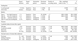
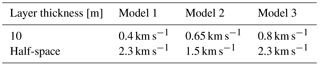
Table 2Three simplified layered vP velocity models at clayey landslides.
4.2 Quakes
4.2.1 Previous observations
Quake signals have been observed in previous studies carried out at clayey landslides. Gomberg et al. (1995, 2011) reported short-duration earthquake-like signals, with clearly discernable, trackable wave packets that they referred to as “slidequakes”. Dominant frequencies of slidequakes were not stated, but can be visually evaluated between 10 and 100 Hz based on the waveforms displayed in Figs. 5 and 6 of Gomberg et al. (2011). Walter et al. (2012) described earthquake-like events with durations of up to 5 s and associated frequency contents of 10–80 Hz, which they also referred as slidequakes after Gomberg et al. (1995). Tonnellier et al. (2013) and Provost et al. (2017) reported quake-like signals with durations of about one second, dominant frequencies around 10 Hz, emergent first arrivals and undistinguishable P and S waves.
4.2.2 Updated classification of quake signals
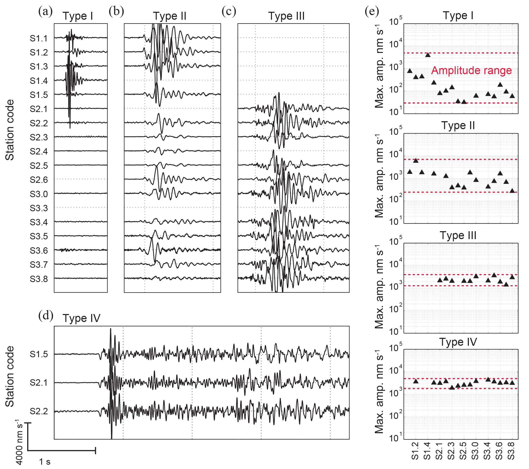
Figure 3Vertical trace seismograms of quake events recorded at SZ10 (see station location and nomenclature in Fig. 1; empty traces correspond to missing or corrupted records). A constant amplitude and timescale are applied to all waveforms (bottom left). (a) Near high-frequency quake type I (29 May 2010, 23:05:05 CEST). (b) Near low-frequency quake type II (26 June 2010, 18:44:55). (c) Moderate distance quake type III (17 June 2010, 15:32:45). (d) Local microearthquake type IV (7 June 2010, 11:24:29). Note the highly coherent successive phases and moderate scattering. (e) Maximum amplitudes (log nm s−1) recorded at individual stations for the four events displayed in (a)–(d). Large amplitude ranges (i.e., important waveform amplitude attenuation, indicated by dashed red lines) enable one to discriminate event types I and II from event types III and IV which typically feature narrow amplitude ranges.
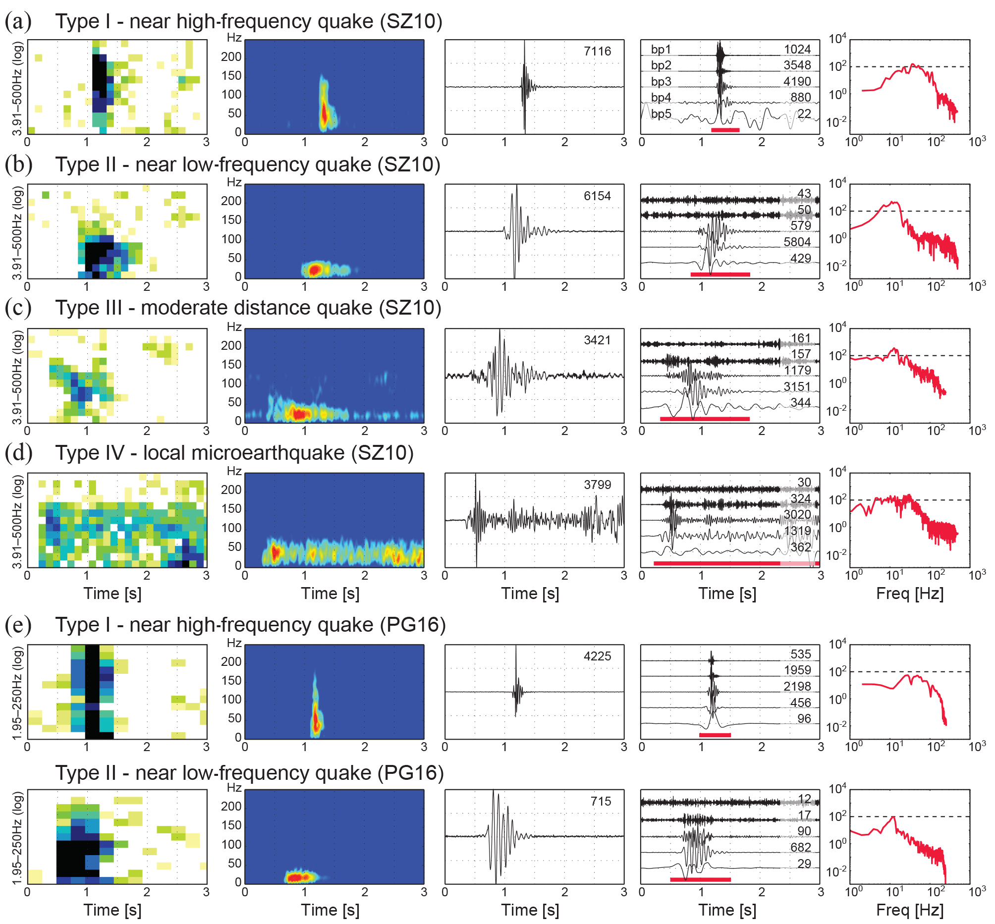
Figure 4(a–d) Seismic features of the highest SNR/amplitude trace of events presented in Fig. 3 and corresponding to type I–type IV quakes. (a) Type I, SZ10, S1.4, t0 29 May 2010, 23:05:04. (b) Type II, SZ10, S1.2, t0 26 June 2010, 18:44:55. (c) Type III, SZ10, S3.0, t0 17 June 2010, 15:32:45.50. (d) Type IV, SZ10, S2.1, t0 7 June 2010, 11:24:29.30. (e) Example of near quakes recorded at Pechgraben. Top: type I, PG16, S2.6, t0 7 November 2016, 22:43:05.50. Bottom: type II, PG16, S1.4, t0 9 November 2016, 01:50:13.
Based on waveform amplitude attenuation pattern, duration and dominant frequency content of the signals, we propose four types of quake events (Table 1; Figs. 3 and 4).
-
Type I – near high-frequency quakes. Signals showed durations of less than 1 s and were only recorded at a few nearby stations, suggesting a nearby source (Fig. 3a). Waveform amplitudes showed strong attenuation (Fig. 3e). Maximum absolute amplitudes of about 10 000 nm s−1 were observed. High-SNR signals feature impulsive onsets. Dominant frequencies of the highest amplitude traces were in the 20–100 Hz range (spectrogram, band-pass filtered waveforms and amplitude spectrum in Fig. 4a and e (upper panel)). P and S phases could not be clearly distinguished; however, successive phases may be identified based on the apparent velocity of trackable wave packets that scale within 0.2–1.8 km s−1.
-
Type II – near low-frequency quakes. Signals showed durations of 1–2 s and were recorded by the complete seismic network with strong amplitude attenuation, suggesting a nearby source (Fig. 3b and e). Maximum amplitudes of a few 10 000 nm s−1 were observed. Dominant frequencies of the highest amplitude signals typically stayed in the 5–50 Hz range (spectrogram, band-pass filtered waveforms and amplitude spectrum in Fig. 4b and e (lower panel)). The signals appeared as prominent and scattered surface waves that could be tracked over the seismic network. P and S phases could not be clearly distinguished; however, successive phases could eventually be discriminated based on the apparent velocity of trackable wave packets that ranged within 0.2–1.8 km s−1.
-
Type III – moderate distance quakes. Signals lasted 2.0–2.5 s and were recorded by the complete seismic network with consistent amplitudes across the seismic network suggesting a source outside of the seismic network (Fig. 3c and e). Most events featured low amplitudes and were recorded just above the noise threshold (100–500 nm s−1). Dominant frequencies were in the 5–50 Hz range, but weak signal energies were typically found within 50–100 Hz at the onset of the events (spectrogram, band-pass filtered waveforms and amplitude spectrum in Fig. 4c). Apparent velocities of scattered wave packets ranged within 1.5–2.0 km s−1. P and S phases were difficult to identify.
-
Type IV – local microearthquakes. Signals had durations of 2–10 s and were recorded by the complete seismic network with similar amplitudes (Fig. 3d–e). Successive phases could be tracked consistently over the seismic network with apparent velocities ranging within 2.0–5.0 km s−1. Dominant frequencies were in the 5–50 Hz range but signal onsets generally displayed energies in the 50–100 Hz range (spectrogram, band-pass filtered waveforms and amplitude spectrum in Fig. 4d). P and S phases could be identified.
4.3 Tremor signals
4.3.1 Previous observations
Various tremor-like signals were observed at clay-rich instabilities. Gomberg et al. (1995, 2011) reported episodes of tremor-like radiation and sinusoidal waveforms lasting tens of minutes and being coherent across the seismic network, which they inferred as ETS (episodic tremor and slip) signals by analogy to ETS signals observed at strike-slip faults. A deeper analysis showed that many of these signals feature gliding spectral lines above 50–100 Hz in the spectrogram. Although gliding frequency tremors have been observed under 20 Hz at volcanoes and are inferred to display change in the source properties (e.g., Hotovec et al., 2013; Unglert and Jellinek, 2015; Eibl et al., 2015, and references therein), gliding harmonics are also characteristic of environmental noise signals produced by moving vehicles such as airplanes or helicopters (e.g., Biescas et al., 2003; van Herwijnen and Schweizer, 2011; Eibl et al., 2015, 2017). There, the gliding harmonics correspond to the Doppler shift produced by a moving source passing a stationary receiver. At Slumgullion landslide, Gomberg et al. (2011) interpreted gliding frequency tremors in the 50–100 Hz range as having been generated by the action of moving vehicles along a distant (several kilometers) road. However, a slide-generated source (slow rupture of faults or materials entrained within the faults like trees or boulders, or slow basal slip) was not excluded for tremor-like radiation devoid of gliding frequency and featuring the highest amplitudes at the seismic network most remote location from the road. These events lasted several minutes and showed dominant energies broadly distributed above 30–50 Hz and diminishing toward the Nyquist frequency at 125 Hz (Gomberg et al., 2011).
At Super-Sauze and Valoria landslides, tremor-like signals lacking clear onsets and with undistinguishable phases were observed with durations of a few seconds to tens of seconds (Walter et al., 2012; Tonnellier et al., 2013; Provost et al., 2017). Spiky, cascading signals are interpreted as rockfalls. Such events feature repeated jolts in the 10–30 Hz range that correspond to the rockfall impacts, as well as a “noise band” in the 30–130 Hz range that is likely generated by fine-grain material flows. These events are normally well recorded across the complete seismic network, with moderate waveform amplitude attenuation and maximum amplitudes reaching 1000–10 000 nm s−1. High-frequency tremor-like signals with durations of less than 20 s and maximum amplitudes under 10 000 nm s−1, featuring drastic waveform amplitude attenuation and, thus, only partially recorded across the seismic network were also observed (Walter et al., 2012; Tonnellier et al., 2013). Walter et al. (2012) showed that the occurrence rate of these signals correlated well with the measurements of an extensometer installed in a fissure and co-located with a 1-C seismometer at Super-Sauze (July 2009). They concluded that such signals must be triggered by fissure formations at the surface of the landslide, but also considered the scratching and grinding of landslide material against (emerging) hard rock crests as a potential source.
4.3.2 Updated classification of tremor signals

Figure 5(a–c) Vertical trace seismograms featuring selected signals of a 40 min long tremor sequence recorded 10 October 2015 between 00:35 and 01:15 at PG15 (see station nomenclature in Fig. 1). Waveforms are normalized to the highest amplitude trace of individual events and maximum absolute zero-to-peak amplitudes are given in nanometers per second on top of each seismogram. Event (a) and (c) are harmonic tremors, event (b) corresponds to an ETS-like event. Note the prominent attenuation of the waveforms and the relatively lower amplitudes of harmonic tremors. (d) Signals published in Walter et al. (2012) and interpreted as a fissure event (top, t0 14 July 2008, 23:48:40) and a rockfall event (bottom, t0 14 July 2008, 23:49:04). Waveforms are plotted using the same timescale as in (a)–(c) to facilitate the signal comparison.
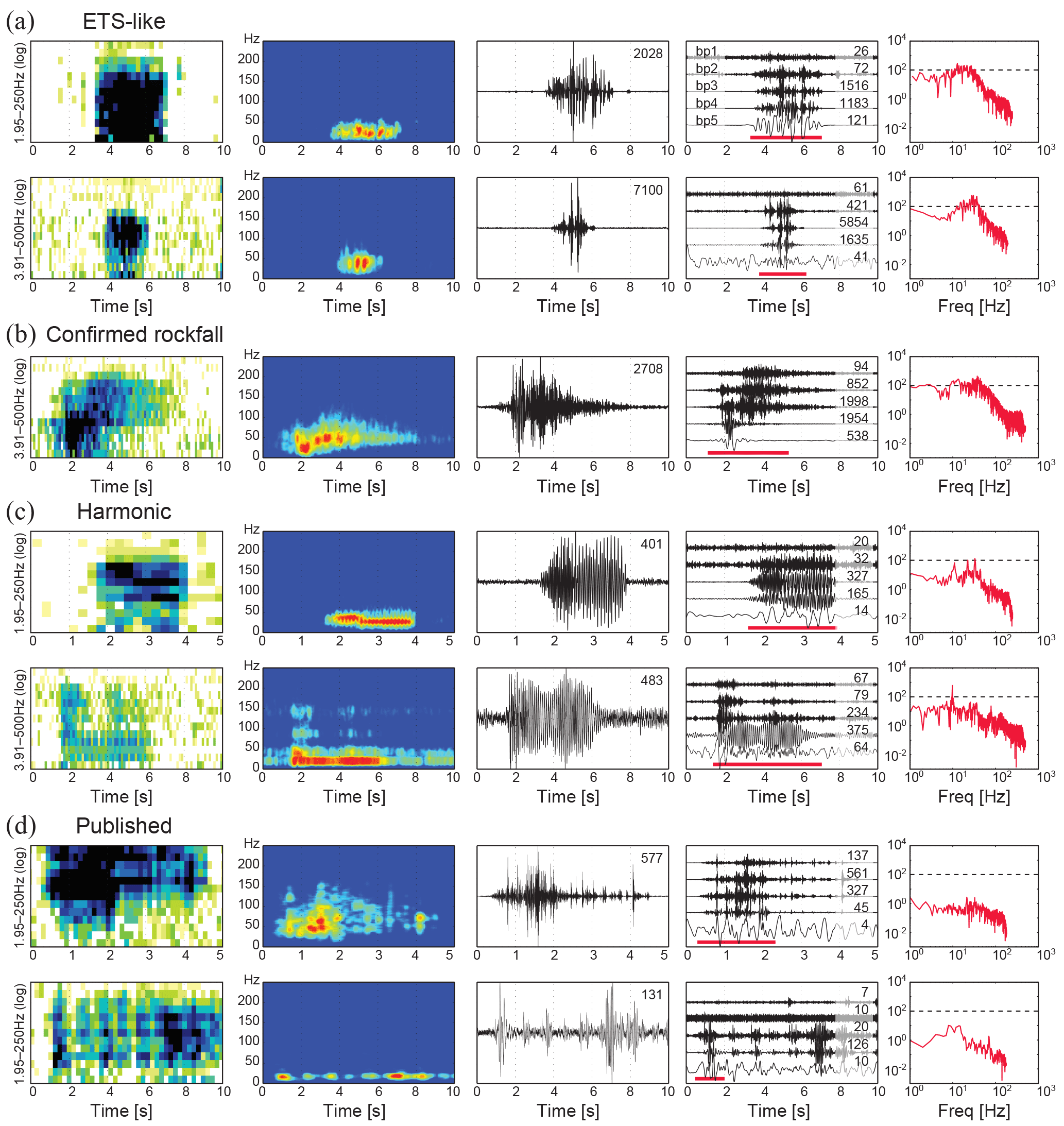
Figure 6Seismic features of moderate duration (< 20 s) tremor signals recorded at Super-Sauze and Pechgraben. (a) ETS-like events. Top: PG15, S2.4, t0 10 October 2015, 00:37:50. Bottom: SZ10, S3.4, t0 5 June 2010, 15:26:35. (b) Confirmed rockfall event at source–receiver distance of 29 m (Rothmund et al., 2017), SZ10, S2.5, t0 4 June 2010, 06:45:20. (c) Harmonic tremors. Top: PG15, S2.6, t0 10 October 2015, 00:36:26. Bottom: SZ10, S2.3, t0 4 June 2010, 20:07:28. (d) Published tremor signals by Walter et al. (2012). Top: fissure event, t0 14 July 2008, 23:48:40. Bottom: rockfall event, t0 14 July 2008, 23:49:04.
As in previous studies, a wide range of tremor-like signals were recorded at SZ10, PG15 and PG16. Short- and medium-duration (< 20 s) events are distinguished from long duration, minute-long lasting sequences of tremor-like radiations (Table 1). While short- and medium-duration events feature trackable wave packets consisting of spikes or jolts, minute-long lasting sequences are characterized by sinusoidal waveforms and gentle rumbles that are difficult to track coherently across the seismic network. Due to the general waveform intricacy and the wide range of observed dominant frequency, finding an unequivocal classification for tremor events is difficult. Based on the literature and searching for consistent observations at SZ10, PG15 and PG16 we propose a typology of tremor events, where landslide-induced tremor-like signals are distinguished from external sources of tremor-like radiations. Among the landslide-induced events, signals potentially generated by deformation and stick-slip within the landslide body are separated, when possible, from tremor-like signals originating from exogenous landslide dynamics such as rockfalls or small debris flows. Since anthropogenic noises share similarities in waveform amplitudes and in spectral content to landslide-induced tremor signals, it is important to gain knowledge about the characteristics of such events for the manual and automatic detection of landslide-induced tremor signals. Therefore, the proposed updated typology of tremor events from this study is as follows:
-
ETS-like signals. Microseismic signals showing similarities to ETS signals at strike-slip faults were observed. ETS-like signals at debris slides are emergent and cigar-shaped, last a few seconds and are strongly attenuated across the seismic network (Fig. 5b and d (top panel)). These signals typically occur in temporal sequences. The dominant frequency of the highest amplitude signals range within 5–50 Hz (spectrogram, band-pass filtered waveforms and amplitude spectrum in Fig. 6a and d (top panel)). Maximum observed absolute amplitudes reach some 10 000 nm s−1; however, most events show amplitudes no higher than a few 100 to 1000 nm s−1. Phases cannot be identified, instead, the waveforms feature repeating, intricate spikes or jolts with prominent scattering. Individual wave packets, which can be tracked, return apparent velocities below 2.0 km s−1.
-
Confirmed rockfall events. Signals generated by rockfalls resemble ETS-like signals (compare Fig. 5b and d with Fig. 6b and d (top panel)). The impacts of falling blocks produce spikes or jolts in the waveforms; loose material saltation and flow combined with the moving character of the source increase waveform intricacy. Signal duration and dominant frequency, as well as waveform amplitude attenuation patterns vary significantly depending on the size of the rockfall event and its distance from the recording seismic network. Apparent velocities derived for individual impact signals remain below 2.0 km s−1. Because rockfalls are exogenic, potential source areas are known from field observations. In addition, the signal source can eventually be caught by field observations or remote sensing. At SZ10, one landslide-induced tremor signal could be matched with a single-marl block failure event captured in high-repetition rate UAV imagery (unmanned aerial vehicle) and optical ground-based images (Rothmund et al., 2017).
-
Harmonic tremors. Signals lasting a few seconds and consisting of narrow frequency band harmonic peaks were observed at SZ10, PG15 and PG16 (Fig. 5a, c and 6c). The main harmonic is generally found around 8–10 Hz, followed by several multiples of lower energies (Fig. 6c, amplitude spectrum). Maximum absolute zero-to-peak amplitudes do not exceed a few 100 to 1000 nm s−1, and most signals lie barely above the noise threshold. At SZ10, harmonic tremors were only observed at single sensors. At Pechgraben, harmonic tremors were detected with various waveform amplitude attenuation patterns across the seismic network, suggesting a non-unique source location origin for these signals. Because of the harmonics, apparent velocities are difficult to calculate. For high-SNR signals, apparent velocities calculated with the first arrivals derived velocities of less than 0.7 km s−1. Harmonic tremors typically occur in minute-long lasting sequences, alternating with ETS-like signals (Fig. 4a–c).
-
Dispersive tremors. Several instances of long-duration (few minute long) dispersive tremor-like signals were detected at SZ10, PG15 and PG16. Due to the dispersive character of the signals, the waveforms and spectrograms feature important variations from one station to another; this rendered the events difficult to detect. Figure 7a shows an example of a dispersive tremor, which was well recorded across the seismic network at SZ10. The high amplitudes (> 20 000 nm s−1) and dominant frequency content above 50 Hz at station S3.7 (spectrogram, band-pass filtered waveforms and amplitude spectrum in Fig. 7a (top panel)) suggested a source origin close to that station. Then, with increasing distance to the most probable source area (source–receiver distances indications above the sonograms in Fig. 7a), the signals showed prominent dispersion and waveform amplitude attenuation. Apparent velocities calculated at the signal onset ranged from 0.3 to 0.5 km s−1, close to the velocity of sound in the air or velocities in the top most layer of the landslide (e.g., Tonnellier et al., 2013). The temporal evolution of the dominant frequency content of the signals and the waveform envelopes, well observed in the spectrograms of Fig. 7 and in the waveforms of Fig. 8a, show similarities to signals produced by mass movement (e.g., Yamasato, 1997; Biescas et al., 2003) or by people walking around the seismic network (waveforms in Fig. 8a–b and spectrogram in Fig. 9a); this suggest a moving source.
-
External sources of microseismic noise and tremor-like radiations. Shallow installation of the seismometers in clayey materials result in important noise contamination of the seismograms, especially in the high-frequency range (> 50 Hz). The variety of events produced by external noise sources is large. Signals range from short to long duration. However, common to all signals is the absence of identifiable successive phases. Individual wave packets are difficult if not impossible to track. Thus, apparent velocities cannot be calculated. Maximum waveform amplitudes can reach several tens of thousands to hundreds of thousands of nanometers per second and waveform amplitude attenuation patterns are incoherent. The most common microseismic signals produced by external source of noise are presented in Figs. 8 and 9. Nearby (< 50–100 m) moving sources such as geophysicists walking around the study areas produce long-duration spiky tremor radiations (Fig. 8b). Typical of such local moving sources is the change towards higher-frequency content of the dominant energies of the signal as the source (the person walking) is approaching the recording station and the change towards lower-frequency content of the dominant energies of the signal as the source gets further away (sonogram and spectrogram in Fig. 9a). Distant moving sources such as airplanes and vehicles, produce long-duration cigar-shaped seismograms and spectrograms with typical gliding harmonics in the 50–200 Hz range (Figs. 7b, 8c and 9b). Beside anthropological noises, many environmental sources of noise were recorded but could not necessarily be distinguished in the absence of additional data at SZ10, PG15, and PG16. Wind bursts, rainfall and storms as well as water streams and bedload transport all produce long-duration tremor-like radiations. Maximum amplitudes can reach several tens of thousands of nanometers per second and waveform amplitude attenuation pattern across the seismic network is incoherent (Fig. 8d). These events illuminate either several frequencies or only specific frequencies in the spectrograms (see also Provost et al., 2017) and the spectrograms are clearly devoid of gliding harmonics (Fig. 9c–d).
5.1 Source location
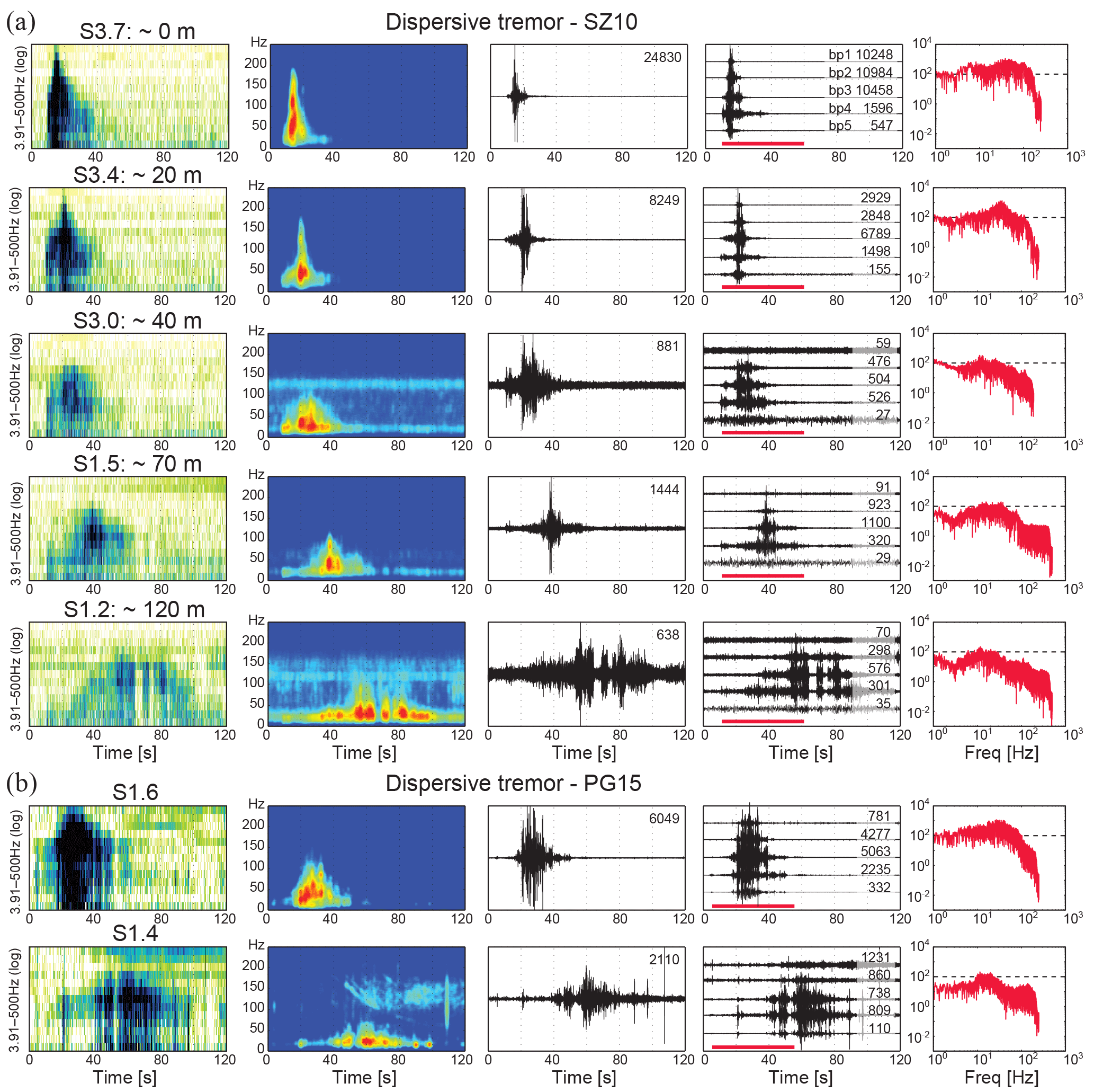
Figure 7Seismic features of two dispersive tremor events recorded at (a) SZ10 at t0 4 July 2010, 00:45:20 and (b) PG15 at t0 8 October 2015, 18:02:08. Stations are indicated on top of the sonogram panels and displayed in (a) and (b) from top to bottom with increasing inferred distance from the most probable source area (SZ10 stations S3.7 and S1.2 are about 120 m distant; PG15 stations S1.6 and S1.4 are about 50 m from one another, so the source–receiver distance could not be estimated). Note noise contamination from an airplane (gliding harmonics in the spectrogram) was very visible at PG15 station S1.4. The airplane signal was well recorded by the complete seismic network, whereas the dispersive event is only seen at array S1 stations.
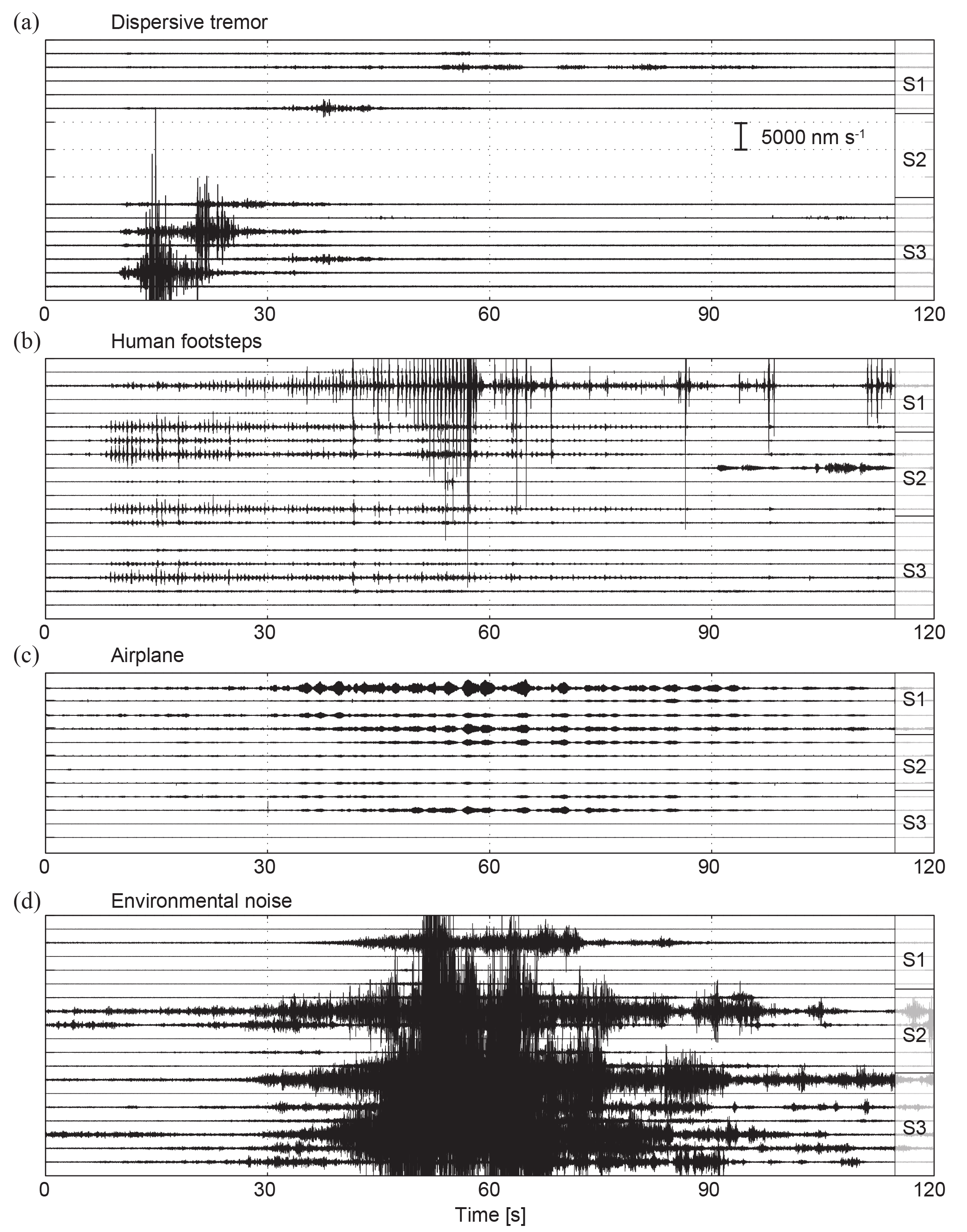
Figure 8Vertical trace seismograms of long-duration tremor-like signals recorded at Super-Sauze and Pechgraben. A constant time and amplitude scale (indicated in a) is applied. (a) Dispersive tremor, SZ10, t0 4 July 2010, 00:45:20. (b) Human footsteps at short distances, SZ10, t0 5 June 2010, 13:08:33. (c) Airplane, PG16, t0 8 November 2016, 04:56:00. (d) Environmental noise, SZ10, t0 9 June 2010, 22:54:10.
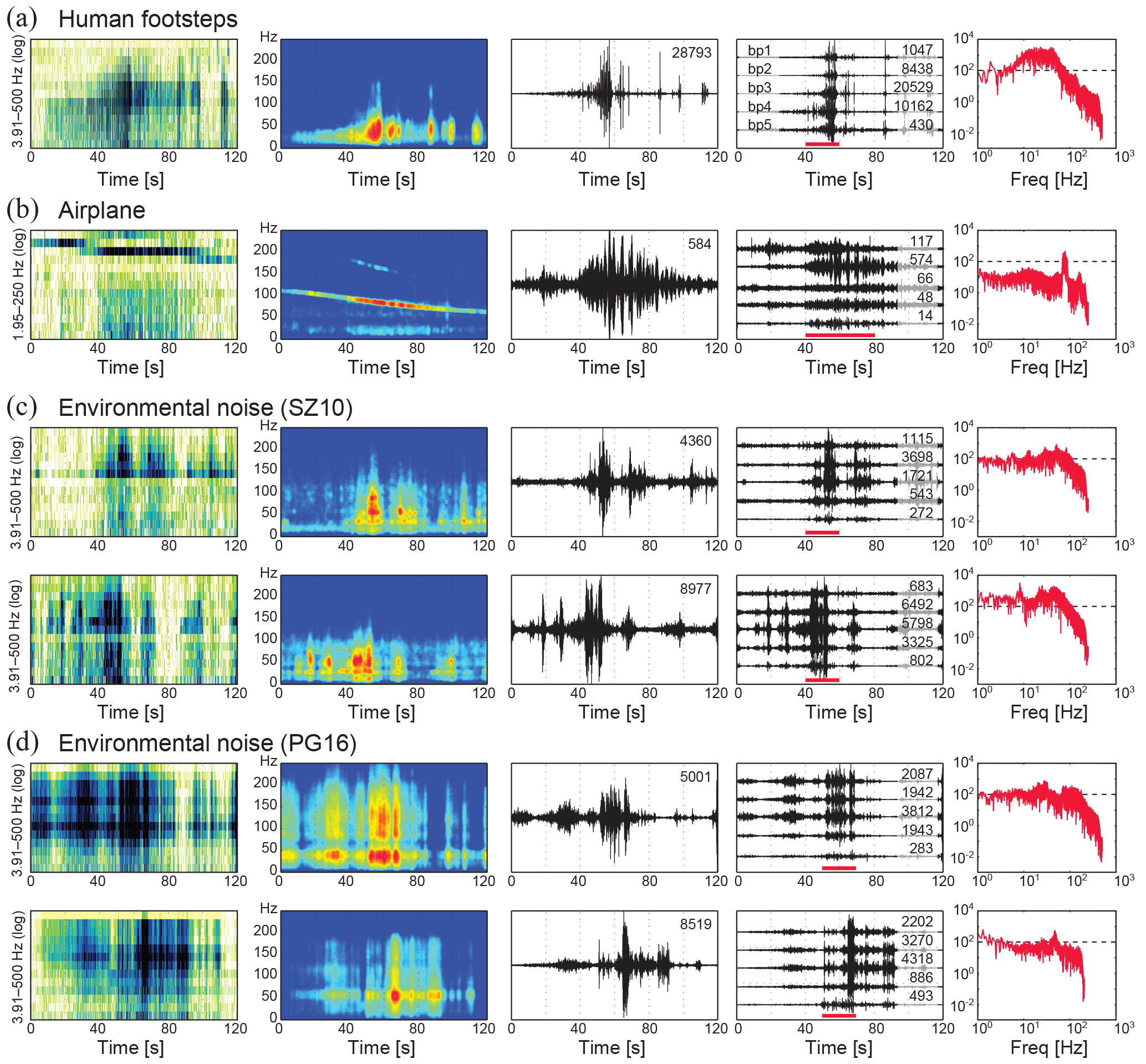
Figure 9Seismic features of the most common external sources of tremor-like radiations. (a) Human footsteps at short distance at SZ10, S1.2, t0 5 June 2010, 13:08:33. (b) Airplane at PG16, S2.1, t0 8 November 2016, 04:56:00 with typical gliding harmonics in the spectrogram. (c) Environmental noise recorded at SZ10, stations S2.3 (top) and S3.8 (bottom) at t0 9 June 2010, 22:54:10 and (d) at PG16, stations S2.1 (top) and S3.1 (bottom) at t0 8 November 2016, 03:00:40.
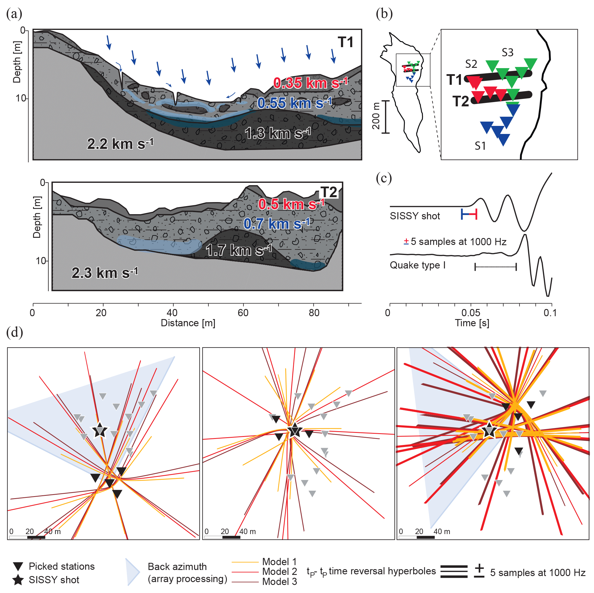
Figure 10Parameters impacting arrival-time based location uncertainties at clayey landslides. (a) Complex seismic velocity structures along two tomographic profiles T1 and T2 at Super-Sauze (modified from Tonnellier et al. (2013) and Gance et al. (2016)). (b) Location of the tomographic profiles T1 and T2 within the seismic arrays S1, S2 and S3. (c) High-quality first arrival of a SISSY calibration shot (top trace, SZ10, S2.2, t0 4 June 2010, 11:56:22) and first arrival of a high-SNR quake type I event (bottom trace, SZ10, 29 May 2010, 23:05:03). Note the higher uncertainties about the onset of the natural event. (d) Graphical location solutions for the SZ10 SISSY calibration shot at station S2.1, 4 June 2010, 11:56:22 derived from first arrivals at individual seismic array S1 (left panel), S2 (middle panel) and S3 inner ring (right panel). Picked stations are indicated by black triangles, beam-processing results are symbolized by shaded light-blue quadrants, time-reversal hyperboles derived with three different velocity models (Table 2) are represented by orange, red and brown lines. In the right panel, bold hyperboles display the effect of ±5 samples' uncertainties offset shifts in first arrivals. Discussion is found in Sect. 5.1.
Seismic velocities and source location quality can be estimated and verified using calibration shots or hammer blows. Calibration shots and hammer blows were carried out at SZ10 and PG16 and could be located with average accuracies of about ±50 m, when using all available first arrivals and back azimuth information with a half-space velocity model. Our results concur with previous results by Tonnellier et al. (2013) at the Super-Sauze landslide, where uncertainties of 40–60 m were estimated for calibration shots carried out within the seismic network. It is worth mentioning that this corresponds to the size of the seismic network and scales with regard to the landslide dimension. Thus, even if the seismic network is dense, locating landslide-induced microseismic sources in clayey landslides and discriminating between a source originating within or outside of the landslide body is challenging due to the following: (1) The velocity structures show drastic variations over short distances (complex material mélange, topography), and also evolve with time (slope deformation, hydrological state). Thus, velocity models are only approximated by tomographic analysis for a specific time (Fig. 10a–b). (2) Scattering and attenuation of the waveforms result in low-SNR onsets where phases are difficult (if not impossible) to identify. (3) The seismic network geometry relative to the source is, in most natural cases, not optimal. (4) With an average station spacing of 5–50 m, as was the case in our study, most landslide-induced microseismic events show no more than four pieces of unambiguous phase information.

Figure 11(a) Maximum absolute zero-to-peak amplitudes with distance to the source of SISSY calibration shots carried out at Super-Sauze 4 June (dots) and 6 July (squares) 2010, and hammer blows (crosses) carried out at Pechgraben, 10 November 2016. Dashed lines indicate log–log regression curves. Note the lower attenuation with dryer conditions. (b) Scatter about the median amplitude (S) of the calibration datasets presented in (a). S values of natural events higher than 200, 1000 and 2000 % are inferred to display source–receiver distances of about 50, 20 and 10 m (t1 t2 t3), respectively.
We used HypoLine (see Sect. 3) to simulate and graphically analyze the contribution of these parameters to the epicentral location solutions of the calibration shots (SISSY, Seismic Source Impulse System, developed by the LIAG, Leibniz-Institut für Angewandte Geophysik, Germany) at SZ10 (Fig. 10). Three layered vP velocity models simplified from Tonnellier et al. (2013) and featuring both higher and lower velocity contrasts between the landslide material and the sedimentary host rock were tested (Fig. 10a–b; Table 2). For each pair of first arrivals, the time-reversal hyperboles (hypolines) were computed at depth zero. To display the weight of phase uncertainties on the epicenter solutions, all hypolines were also computed for two shifted values of the first arrival by ±5 samples (Fig. 10c). An epicenter solution is found at the highest concentration of hyperboles intersections (see Joswig, 2008 and Vouillamoz et al., 2016 for details). The exercise was carried out for the three velocity models and the resulting epicenter solutions were analyzed for different station combinations. Figure 10d shows the results obtained when using first arrivals of the three seismic arrays individually. The outcomes of this analysis can be summarized as follows:
-
The applied velocity model has a low impact on the epicentral solution (a few meters) within the considered station network or at small distances. However, outside of the seismic network, solutions diverge significantly.
-
Five samples (±) uncertainties at 1000 Hz correspond to a high-quality phase onset pick in routine earthquake catalogs (e.g., Diehl et al., 2009). Such high-quality phase onsets derive consistent solutions within the considered station network, but the solutions also diverge significantly outside of the considered seismic network.
-
First arrivals of natural sources are of lower quality than those of calibration shots (Fig. 10c). Lower quality onsets have an important impact on the epicentral solutions. At ±20 samples (±0.02 s), a mathematical solution is no longer found!
-
The seismic network geometry relative to the source has the most significant influence on the location solution. The epicenter is resolved with uncertainties of about 20 m when using a set of stations surrounding the calibration shot (Fig. 10d (central panel)); however, the potential location solutions are biased by 50 m or more when using a station network that does not surround the source (Fig. 10d (left and right panels)).
-
First arrivals at stations in tripartite configurations derive three zones of high-density hyperbole intersections that cannot be discriminated without additional constraints, such as back azimuth information (beam-processing).
-
Complex velocity structures and the resulting waveform scattering impedes array processing, and back azimuth information can be significantly biased. The calibration datasets at Super-Sauze and Pechgraben derive uncertainties in the order of one quadrant (±45∘) for well constrained beams (using high correlation values of four and more coherent waveform spikes), for sources located 50–100 m outside of the seismic mini-array.
-
Sources originating within the seismic network return incoherent array processing and back azimuth data.
Thus, it can be concluded that approximation in the velocity model, low-quality first arrivals and non-optimal seismic network geometry at clayey landslides, result in natural source location uncertainties ranging from tens of meters for sources originating within the seismic network to hundreds of meters for sources originating outside of the seismic network. Consequently, the risk of including biased data in maps of landslide-induced microseismicity is high. Moreover, the estimation of the local magnitude of a microseismic event has a logarithmic dependence on the source–receiver distance. Thus, high uncertainties (> 50–100 m) held in the source location can affect the magnitude calculation by several orders of magnitude units.
5.2 Amplitude attenuation pattern to constrain source–receiver distance
Because of the high uncertainties returned by arrival-time based approaches to event location, the drastic attenuation of waveform amplitude observed within the landslide body was used to constrain the source proximity of near-source area landslide-induced microseismic events. This information was then used in the calculation of events' local magnitudes. Distance attenuation data from the SISSY calibration shots and hammer blows at Super-Sauze and Pechgraben show that signals are strongly attenuated within the first 50 m. The water content of the landslide material influences the waveform amplitude attenuation: signals are less attenuated when dryer conditions prevail (Fig. 11a). This observation is consistent with laboratory experiments (e.g., Koerner et al., 1981). To quantify the waveform amplitude attenuation pattern of an event, we use the scatter about the median amplitude, S, which we compute for each trace that recorded a signal as follows:
where Asta is the station maximum absolute vertical trace amplitude of the signal in nm s−1 and Med(Asta) is the median value of all Asta where the signal was recorded. S values computed for the calibration dataset of Fig. 11a show a drastic diminution with increasing source–receiver distance (Fig. 11b). Based on these observation, we use maximum S values of landslide-induced microseismic events to approximate source–receiver distances. We infer that S values higher than 200 % correspond to source–receiver distance of less than about 50 m. At smaller distances, we selected thresholds (in an arbitrary, but conservative way) of 1000 and 2000 % to correspond to source–receiver distances of about 20 and 10 m from the recording station, respectively. Source distances of natural events for which S values remain below 200 % are considered uncertain. Since S values of teleseisms and distant earthquakes were observed to be very stable (< 100 %), no correction for site effects was applied. Among the inferred landslide-induced microseismic events (quakes and tremors), 48 % of events at SZ10, 24 % at PG15 and 39 % at PG16 feature at least one station with a scatter about the median amplitude value above 200 %. With an estimated source-receiver distance of less than about 50 m, these events can be reasonably assumed to have originated within the landslide body or at its edges (see Sect. 6.3); therefore, they are used in the local magnitude catalog of landslide-induced microseismic events.
5.3 Calibrating the local magnitude (ML) scale at clayey landslides
Richter (1958) defines the earthquake local magnitude scale ML as follows:
where AWA is originally half of the maximum peak-to-peak amplitude (in microns) recorded on a Wood–Anderson (WA) seismograph, and log10(A0) is the distance attenuation function i.e., a correction applied for the attenuation of the waveforms with distance. The scale is defined so that a ML 3 earthquake records a 1 mm peak amplitude on a WA seismograph at a source–receiver distance of 100 km. The distance attenuation function of the ML scale has been empirically calibrated for earthquakes in many regions around the world (e.g., Bakun and Joyner, 1984; Hutton and Boore, 1987; Stange, 2006; Edwards et al., 2015); however, standard calibrated source–receiver distances range from 10 to 1000 km (Fig. 12a). Therefore, these distance attenuation functions are unappropriated for near-source area microseismic events at landslides. Wust-Bloch and Joswig (2006) calibrated a distance attenuation function within 30–300 m for sinkhole events in the Dead Sea valley. Its slope is very similar to extrapolated distance attenuation functions at distances of less than 1 km (Fig. 12b).
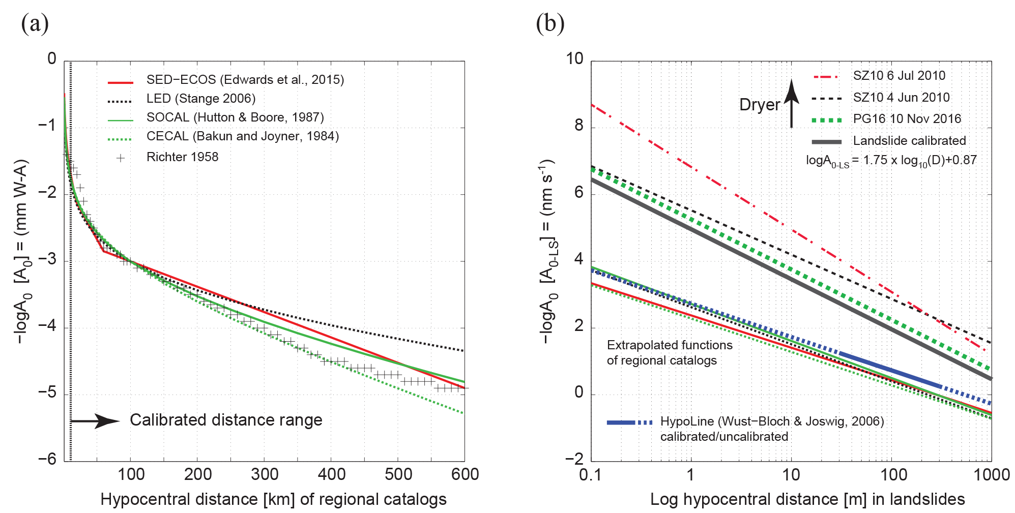
Figure 12(a) Distance attenuation functions (−log(A0)) of ML scales empirically calibrated for regional earthquakes with source–receiver distances between 10 and 600–1000 km. (b) Log–log zoom in of the valid source–receiver distance range of microseismic observations at clayey landslides. The HypoLine distance attenuation function, which was calibrated between 30 and 300 m in the Dead Sea valley (Wust-Bloch and Joswig, 2006) is very similar to the projection of the regional ML scales. The distance attenuation regression curves derived from the SISSY calibration shots and hammer blow data (see Fig. 11) project into the upper area of the graph, all with steeper slopes (displaying stronger attenuation) than the regional ML scales. The landslide calibrated distance attenuation function applies an average slope of 1.75 with an intercept of 0.87. Note that regional ML scales use displacement amplitudes in WA in millimeters, whereas ML−LS scale is calibrated using velocity readings in nanometers per second; hence a direct comparison of these curves is not straightforward. Discussion is found in Sect. 5.3.
We calibrated ML in clayey landslides (ML−LS) by defining the slope and the intercept of the simplest form of the distance attenuation function:
where log10(A0−LS) is the distance attenuation function in landslides and D is the source–receiver distance in kilometers. The slope is defined using the MATLAB® logfit function (© 2014, Jonathan C. Lansey), which returns a regression in the form Y=10interceptXslope for the calibration datasets presented in Fig. 11a. An average slope value of −1.75 is found for the different regression curves and taken for log10(A0−LS) (Fig. 12b).
The intercept of log10(A0−LS) is then calculated as follows:
-
The theoretical moment magnitude Mw of a SISSY calibration shot is estimated following the Gutenberg–Richter magnitude energy relation, where log.8 – E being the radiated seismic energy in ergs. Using E=240 kJ (SISSY product information sheet), we find .39.
-
Following Deichmann (2017), we derive the ML of a SISSY shot as .58.
-
The intercept of log10(A0−LS) is found using .58 with the mean slope of the regression curves (−1.75) and the average maximum absolute vertical trace zero-to-peak amplitude of the calibration shots at 1 m of source–receiver distance: (ALS=5e106 nm s−1).
The calibrated local magnitude scale ML−LS in clayey landslides is finally expressed as
where ALS is the maximum absolute vertical trace zero-to-peak amplitude of the signal in nm s−1 and D is the source–receiver distance in kilometers.
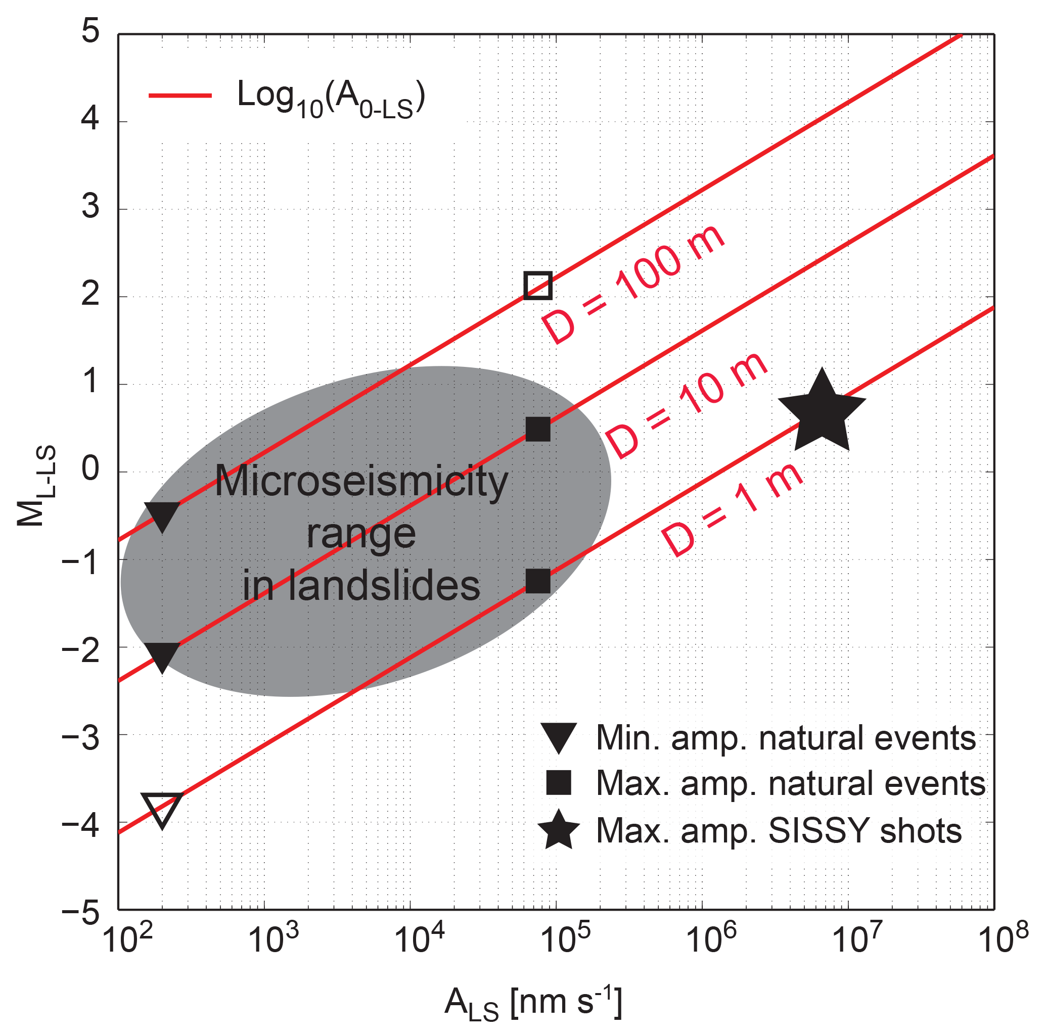
Figure 13ML−LS as a function of amplitude reads at 1, 10 and 100 m source–receiver distances. The star indicates the average maximum amplitude read of SISSY calibration shots at 1 m of distance that corresponds to ML−LS 0.58. Minimum and maximum signal amplitudes observed for landslide-induced signals are symbolized by triangles and squares, respectively. Empty symbols indicate lower probability valid distances of low and high amplitude values. A reasonable field of the potential ML−LS of landslide-induced microseismic events is outlined by the shaded ellipse.
The calibrated distance attenuation curves are steeper than the average slope of regional earthquakes' −log10(A0) curves (Fig. 12b). However, since no simple relation exist between AWA in millimeters (as used in the calculation of standard ML) and ALS in nanometers per second (as read on a detection trace in landslides), the comparison of standard distance attenuation functions log10(A0) with log10(A0−LS) is not straightforward. Well displayed in Fig. 12b, is the strong influence various water saturation levels of landslide material prevailing during the different calibration measurements, which can result a bias of one order of magnitude or more at distances smaller than 100 m. The range of potential ML of landslide-induced microseismic events is evaluated in Fig. 13. ML−LS is plotted as a function of the amplitude read in nanometers per second using log(A0−LS) for three source–receiver distances (1, 10 and 100 m). Considering the range of observed signal amplitudes, the graphic shows that landslide-induced microseismicity must scale within about −3.0 < ML−LS < 1.0. This agrees with the potential magnitude range, which can be inferred from field observations and assumptions, where active seismogenic structures are expected to fall in the decimeter to meter range.
6.1 Passive seismic monitoring at clayey landslides
Progress in environmental seismology is driving geophysicists and seismologists into more and more exotic terrains. In this section we provide a few comments about seismic network deployment and optimization at active landslides, based on our experience. Tripartite seismic arrays are well-suited for apparent velocity and back azimuth determination of an incoming signal (e.g., Joswig, 2008; Vouillamoz, 2015; Sick, 2016), and provide key information about source location. Such arrays were used at both Super-Sauze and Pechgraben; however, due to the rugged and obstructed terrain, as one encounters at any active landslide site, it was not possible to deploy the tripartite arrays with their theoretical optimal geometry (equilateral triangles). Nevertheless, the arrays proved successful in deriving back azimuth and apparent velocity information, using a sampling rate of 400 Hz or more. The optimal array aperture was found between 5 and 10 m. Larger inter-distances at stations resulted in many small landslide-induced microseismic events not being recorded by all stations, thereby limiting their characterization. Seismic stations housed and installed on a concrete slab for long-term monitoring showed signals similar to those registered by seismic stations simply buried within the ground for short-term monitoring. No significant difference was observed between landslide-induced microseismic signals recorded by stations installed on the active part of the landslide and stations placed on the stable areas surrounding the landslide. Therefore, future efforts may consider installing the seismic network on the stable areas surrounding the landslide for long-term monitoring campaigns to avoid seismic station displacement and tilting.
6.2 Landslide-induced microseismic events detection and classification
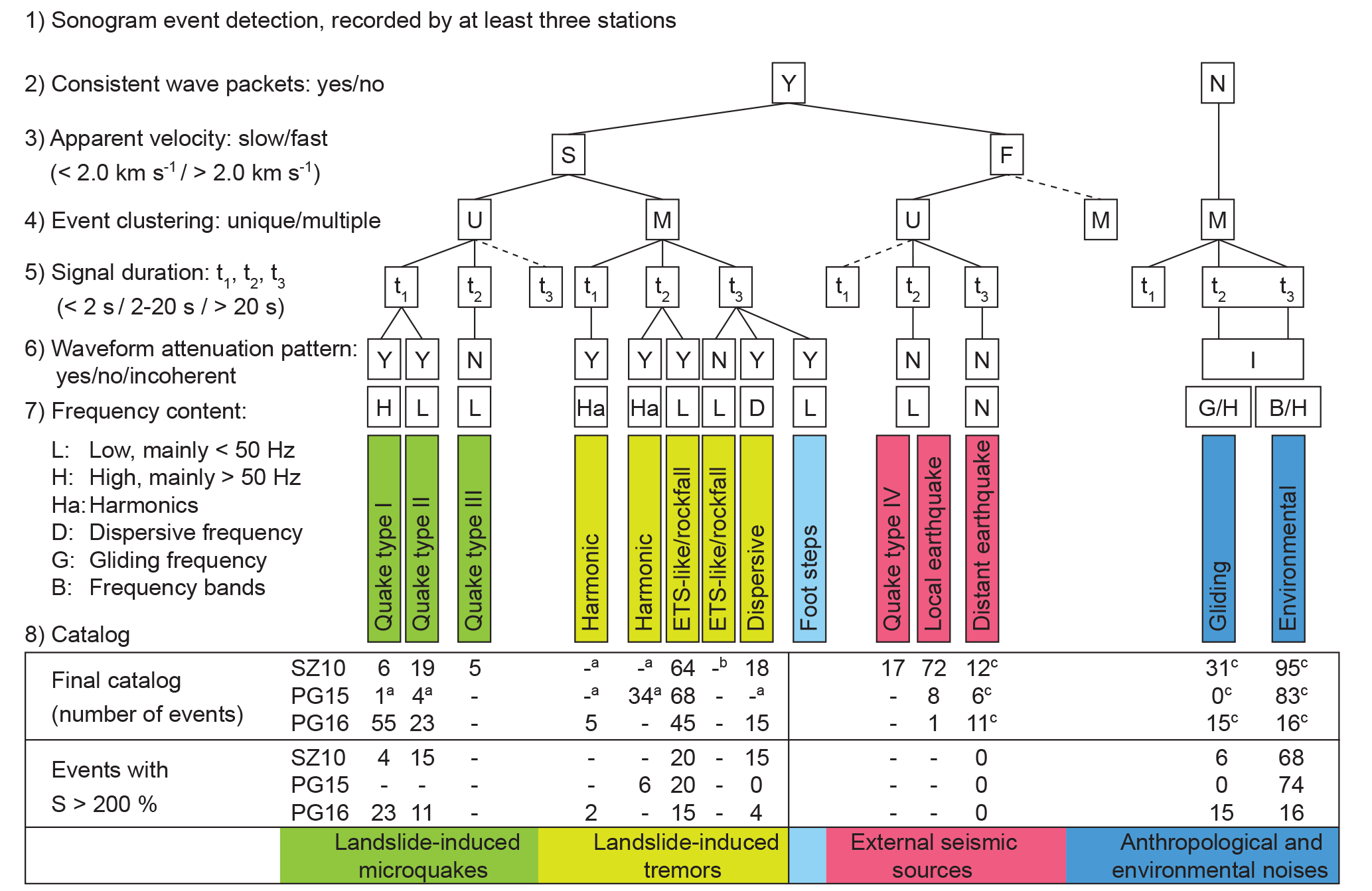
Figure 14(1–7) Final decision-tree for microseismic event classification at clayey landslides. (8) Catalog with number of detection for each class (top frame) and number of near-source area events with S > 200 % (bottom frame). Indices indicate (a) fields in which such events were detected, but recorded at less than three seismic stations; (b) fields were such events were observed by other fields campaigns (e.g., Walter et al., 2012); and (c) fields unrelated to the landslide microseismicity, where only the higher SNR events were catalogued. Discussion is found in Sect. 6.3.
Automatic detection algorithms are suitable for well-known routine seismic signatures but fail for unknown and unexpected low-SNR microseismic events. Therefore, in order to gain knowledge about existing landslide-induced microseismic event signatures we used an enhanced visualization alternative, where continuous seismic data were screened in the form of sonograms for visual pattern recognition (Joswig, 2008; Sick et al., 2012; Vouillamoz et al., 2016). We summarize the final decision tree applied to the microseismic event classification at clayey landslides in Fig. 14, using a minimal number of simple seismic features (described in Sect. 3): (1) a detection was declared for microseismic events observed at a minimum of three seismic stations. (2) A initial distinction was made between microseismic events featuring distinct wave packets and events consisting of incoherent sinusoidal signals. The latter gather external sources of tremor-like radiations such as gliding events (airplanes) and environmental noise (rain fronts, storms, wind, creeks and so on). (3) The decisive discriminating parameter for landslide-induced microseismic events is the slow apparent velocity of distinct wave packets. Events returning fast apparent velocities correspond to external seismic sources, i.e., near, local, regional earthquakes and teleseisms. (4) Unique events were distinguished from multiple events featuring repeated high-energy jolts, making the separation between microearthquake (type I, II and III) and landslide-induced tremors (ETS-like, rockfall, harmonic and dispersive). (5) The signal duration reflected the source proximity for unique events (the shorter the signal the closer the source). For multiple events, it provided an indication about the source size (longer signals carry more energy). (6) Important waveform amplitude attenuation patterns (S > 200 %) were evidence of a nearby source (source–receiver distance of less than about 50 m) (Sect. 5.2). This is consistent with the observation that near, local and regional earthquakes do not show S values above 200 %. Incoherent waveform amplitude patterns were typically observed for external sources of tremor radiations (gliding and environmental signals). (7) Characteristics in the frequency content such as dominant frequency above 50 Hz (e.g., band-pass filtered waveforms in Fig. 4a), harmonics (e.g., unfiltered waveform and amplitude spectrum in Fig. 6c), dispersive dominant energies (e.g., spectrograms in Fig. 7a), gliding frequencies (e.g., spectrogram in Fig. 8b) or multiple frequency bands (e.g., spectrograms in Fig. 8c) enabled the last specification regarding the end-member event classes. (8) Detected events were gathered in a final catalog of microseismicity at clayey landslides.
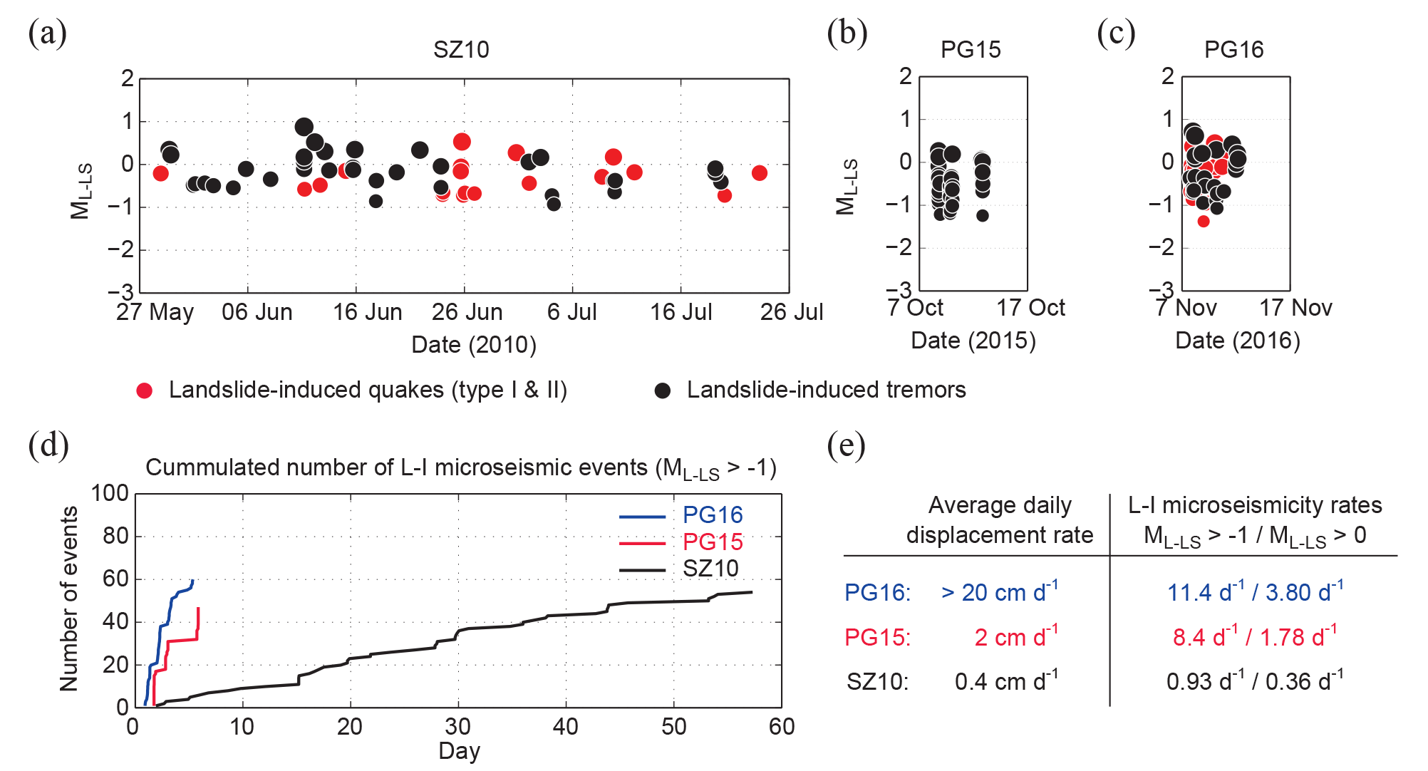
Figure 15(a–c) Temporal distribution of ML−LS for near-source area (< 50 m) landslide-induced microseismic events at SZ10 (a), PG15 (b) and PG16 (c). Red circles show quake events type I and II and black circles indicate landslide-induced tremors (ETS-like, rockfall, harmonic and dispersive with S> 200 %). The timescale is constant in all plots. (d) Cumulative number of landslide-induced microseismic events with S > 200 % curves for ML−LS > −1 events. (c) Daily landslide-induced microseismicity rates for ML−LS > −1 and ML−LS > −0 show an increase with higher average daily displacement rates.
The shallow installation of seismic stations in the landslide body results in a high level of noise contamination in the data, rendering the detection and distinction of landslide-induced microseismic events and other environmental (or anthropological) sources difficult. Seismic signal signatures of proximal sources show important variations among different stations' records, as a function of changing source–receiver distance (e.g., Figs. 3a–b, 5a–c and 7). Despite this, many landslide-induced microseismic events were observed in temporal sequences, suggesting a common source process; although, a cross-correlation analysis performed in the time domain (1–30 Hz band-pass filter) returned no evidence of similar events among the considered sequences. This stresses the complexity and variability of signals radiated by near-source area microseismic processes at clayey landslides. Individual microseismic sources can also occur simultaneously on a complex debris slide; therefore leading to time-overlapping tremor signals with hybrid characteristics, where individual source radiations cannot be unambiguously separated. For example, several quake doublets (type II and III), similar to short-duration ETS-like signals were observed at both landslides. At Pechgraben, frequent near quakes (type I and II) featuring short-duration harmonics were observed. Thus, we conclude that an unequivocal classification of landslide-induced microseismic signals is possible for well-defined, high-quality end-member signals. For complex and hybrid events, input from the analyst is still required and larger datasets are needed, in particular to train automated classifiers.
6.3 Landslide-induced microseismic event location and interpretation
Due to the high uncertainties – scaling with the landslide dimension itself – of arrival-time based source location of landslide-induced microseismic events (Sect. 5.1), the source–receiver distance of landslide-induced microseismic events was qualitatively constrained; this was undertaken using amplitude information and no maps of landslide-induced microseismicity were produced. Events featuring S values above 200, 1000 and 2000 % were inferred to have been recorded at a source–receiver distance of less than about 50, 20 and 10 m, respectively, according to calibration tests performed at both landslides (Sect. 5.2). For these near-source area microseismic events, observations of high-SNR signal spectral content above 50 Hz in the band-pass filtered waveforms or in the amplitude spectrum corroborated a nearby source.
Quake events are inferred to be generated by a single rupture process. Type I and type II quakes feature S values above 200 % and signal durations of less than 2 s. Thus, they are considered to be generated over distances of less than 50 m. The slow apparent velocities (< 2.0 km s−1) of the signals are consistent with velocities estimated for clay-rich landslide material (Williams and Pratt, 1996; Tonnellier et al., 2013) and corroborate a source originating within or at the edge of the landslide body. However, one cannot discriminate between the two, because location uncertainty is too high and depth estimation is not possible. S values above 1000 %, higher-frequency content, shorter signal duration and few station records of type I events (Fig. 4a and e) likely reflect a small and very close source (< 10–20 m). Low-frequency content and longer duration of type II events may account for slower rupture velocity and larger rupture area (Fig. 4b). Type III and type IV events feature S values which are below 200 % and represent a continuous transition of quake events recorded at larger source–receiver distances. The higher apparent velocities of wave packets of type IV events and the consistent signal amplitudes of well distinguishable successive phases across the seismic network suggest a source origin outside of the landslide body in the host rock.
The complexity and frequent hybrid characteristics of observed tremor signals make their interpretation challenging. Previous studies interpreted ETS-like signals as being generated by stick-slip (near-repeating quakes) at shear boundaries of the landslide or through fissure development or clogging at the landslide surface (e.g., Gomberg et al., 2011; Walter et al., 2012; Tonnellier et al., 2013). At Super-Sauze and Pechgraben, ETS-like events were mainly observed to occur in temporal sequences; at Pechgraben, alternately with harmonic tremors. Models to explain harmonic tremors include resonance of fluid/gas driven cracks (e.g., Chouet, 1988; Schlindwein et al., 1995) as well as stick-slip (i.e., swarms of small repeating earthquakes) (e.g., Helmstetter et al., 2015; Lipovsky and Dunham, 2016). Therefore, we postulate stick-slip episodes as the most common source of ETS-like and harmonic tremor signal sequences but cannot exclude fissure formation or clogging as mechanisms which produce ETS-like signals. Rockfall events produce signals consisting of spikes and jolts, in some instance very similar to ETS-like tremors. Since potential source areas of rockfall can be observed in the field, multiple-spike microseismic signals returning back azimuth towards such areas can be classified as rockfall signals with good certainty. However, in the absence of additional constraints, an unambiguous classification of rockfall and ETS-like signal can be difficult, in particular when the signals are of low-quality. The dispersive character of waveforms and the dominant frequencies of dispersive tremors suggest a moving source (Sect. 4.3.2). Animals as a potential moving source can be excluded with good certainty, as signals triggered by animals show spikier patterns than human footsteps (Figs. 8b and 9a). The inferred source area of dispersive tremors is difficult to access at Super-Sauze and is extremely marshy at Pechgraben; furthermore, no animals or animal traces were be observed during the daytime. Debris flows were neither observed in the field nor in daily ground-based and UAV imagery and photo-monitoring in the affected areas. At SZ10, a secondary rotational slide and the opening of crown cracks were observed near the inferred source area during the signals detection period. Such a source mechanism would be compatible with field observations made in the potential source area of dispersive tremors at Pechgraben. Thus, we postulate rotational sliding initiation and/or opening of crown crack(s) as a potential source trigger for the dispersive tremors.
6.4 Landslide-induced microseismicity rates
Only near-source area quakes (type I and II) and tremor events (ETS-like, rockfall, harmonic and dispersive) with S > 200 % were used in the ML−LS catalog of landslide-induced microseismicity. This catalog was used to evaluate average daily rates of landslide-induced microseismicity to be compared to average daily displacement rates of the three seismic campaigns (Sect. 2). Figure 15 shows the temporal ML−LS distribution of the near-source area landslide-induced microseismic events for SZ10 (a), PG15 (b) and PG16 (c) and the cumulated number of event curves with ML−LS > −1 (d). The corresponding average daily landslide-induced microseismicity rates, for ML−LS > −1 and ML−LS > 0, show an increase with increasing average daily displacement rates of the three campaigns (Fig.15 (e)). No relationship was found between the energy radiated by local and regional earthquakes (maximum vertical trace absolute amplitude) and the occurrence of landslide-induced microseismic events. At all campaigns, temporal clustering of near-source area landslide-induced microseismic events was observed, especially for tremor signals. Sequences typically lasted a few minutes to a few hours and were followed by quiescent periods. However, higher resolution displacement data (< daily) is required to better decipher a potential correlation between displacement rates and landslide-induced microseismicity.
In this study, we propose a unified typology of microseismic signals observed at slow-moving clay-rich debris slides by comparing passive seismic recordings of three campaigns carried out at two landslides and using similar published case studies as a benchmark. The highly heterogenous and water-saturated states of the material within the slides result in strongly attenuated and scattered waveforms. Signals generally consists of complex and intricate surface waves, where P and S phases cannot be clearly distinguished and successive phase (or wave packet) onsets are difficult, if not impossible to pick. Therefore, simple waveform and spectral attributes of the signals were used for the classification (Sect. 3 and Fig. 14). The principal discriminating parameters we find to differentiate landslide-induced microseismic signals from unrelated external sources are as follows: (1) the low apparent velocity (< 2 km s−1) of trackable wave packets that applies for landslide-induced signals generated at source–receiver distances of 0–500 m (estimated); and (2) the prominent and consistent waveform amplitude attenuation patterns of near-source area events across the recording seismic network (Sect. 5.2). Despite the complexity of the waveforms, comparable landslide-induced microseismic signals were detected at both landslides, suggesting that similar microseismic source processes are taking place and that the method used is scalable and reproducible. Two main classes of landslide-induced signals were found: (1) quake-like signals and (2) a variety of tremor signals (Sect. 4.2–4.3). Because arrival-time based approaches to event location at clayey landslides result in an unacceptable level of location uncertainty, waveform amplitude attenuation patterns were used to better constrain source–receiver distances. This was undertaken by applying a distance attenuation function calibrated for clayey landslides, so that ML−LS could be computed for near-source area events (< about 50 m)(Sect. 5.3). Results show an increase in daily landslide-induced microseismicity rates with higher average daily displacement rates. Although much attention was paid to deriving unbiased magnitude catalogs, uncertainties are still high. In addition, the catalogs may be incomplete in the lower magnitude range due to incomplete datasets (see Sect. 2). Consequently, we did not derive b values.
Since passive seismic methods alone do not allow for a detailed characterization of microseismic source processes taking place at clayey landslides, seismic data should be supplemented with high spatial–temporal resolution remote sensing, geodetic, geotechnical, geophysical, meteorological and hydrological measurements. A major inconvenience is that ground-based measurements on landslides during the day result in high anthropological noise levels, corrupting a significant part of daytime seismic measurements. The seismic monitoring of SZ10, PG15 and PG16 was part of multidisciplinary field experiments and the future of this study involves a detailed comparison of microseismic measurements with the other acquired datasets. The aim of this work will be to precisely evaluate the degree to which the main limitation of passive seismic monitoring (high spatial uncertainty of the detected microseismic events and hence speculative sources characterization) can effectively be compensated for by remote sensing and other geodetic and geotechnical information. The landslide-induced microseismic event catalog also provides an initial signal library with which to train future automatic detection systems and classifiers of complex and hybrid microseismic signals at clayey landslides. In addition to the “random forest” supervised classifier already implemented by Provost et al. (2017) at Super-Sauze, unsupervised pattern recognition (e.g., Sick et al., 2015) or hidden Markov models (e.g., Hammer et al., 2012, 2013) should be tested and success rates as well as method reproducibility and scalability benchmarked.
The Super-Sauze and Pechgraben passive seismic datasets used in this study are stored at the Institute of Geophysics of the University of Stuttgart, Germany, in SEG-2 and MSEED data format. Requests to the data as well as the catalog of microseismic events can be addressed to the authors. Computations and plots were carried out in MATLAB® (https://www.mathworks.com/products/matlab.html, last access: 10 November 2017) under a campus license of the University of Stuttgart.
NV designed and performed the seismic field campaigns of Pechgraben 2015 and 2016 and processed the seismic data of Pechgraben 2015 and 2016 and Super-Sauze 2010. SR helped in the design and data acquisition of the seismic campaigns of Pechgraben 2016 and Super-Sauze 2010. She supported the seismic data processing and significantly contributed to the writing of this paper. MJ originated the multi-approach field campaign at Super-Sauze 2010. He hosted the postdoc project of NV and supported this research with discussion threads.
The authors declare that they have no conflict of interest.
This article is part of the special issue “From process to signal – advancing environmental seismology”. It is a result of the EGU Galileo conference, Ohlstadt, Germany, 6–9 June 2017.
This work was funded by an early postdoc mobility fellowship of the SNSF
(Swiss National Science Foundation, grant P2FRP2_158749).
Birgit Jochum, David Ottowitz and Robert Supper of the Geological Survey of
Austria in Vienna are warmly acknowledged for sharing datasets and providing
insightful tips and help with the field work in Pechgraben. Jon Mosar of the
Institute of Earth Sciences of the University of Fribourg, Switzerland is
thanked for lending seismometers and dataloggers for the Pechgraben seismic
campaigns. The authors are very grateful to Clément Hibert,
Jean-Philippe Malet and Floriane Provost of the EOST, University of
Strasbourg, France, for fruitful inputs to this project as well as for
sharing datasets and codes. The authors thank Marco Walter, Ulrich
Schwaderer and Patrick Blascheck of the Institute for Geophysics (IfG) of
the University of Stuttgart for their support at Super-Sauze 2010 seismic
monitoring campaign and their help in the microseismic data pre-process.
Juan-Carlos Santoyo Campus (IfG, University of Stuttgart) is warmly thanked
for his essential participation in the 2015 Pechgraben field campaign. The
authors would also like to acknowledge and express gratitude to the editor, Fabian Walter
(Laboratory of Hydraulics, Hydrology and Glaciology, ETH-Zurich,
Switzerland) and the two reviewers, Emma Suriñach (Department of Earth
and Ocean Dynamics. Faculty of Earth Sciences. University of Barcelona (UB))
and Andreas Köhler (Department of Geosciences, University of Oslo,
Norway) for their thorough reviews of this manuscript which have help to
improve the paper.
Edited by: Fabian Walter
Reviewed by: Emma Surinach and Andreas Köhler
Bakun, W. H. and Joyner, W. B.: The ML scale in Central California, B. Seismol. Soc. Am., 74, 1827–1843, 1984.
Battaglia, J.: Location of seismic events and eruptive fissures on the Piton de la Fournaise volcano using seismic amplitudes, J. Geophys. Res., 108, 2364, https://doi.org/10.1029/2002JB002193, 2003.
Battaglia, J., Aki, K., and Ferrazzini, V.: Location of tremor sources and estimation of lava output using tremor source amplitude on the Piton de la Fournaise volcano: 1. Location of tremor sources, J. Volcanol. Geoth. Res., 147, 268–290, https://doi.org/10.1016/j.jvolgeores.2005.04.005, 2005.
Beard, F. D.: Predicting slides in cut slopes, Western Construction, San Fransisco, 36, 72 pp., 1961.
Biescas, B., Dufour, F., Furdada, G., Khazaradze, G., and Suriñach, E.: Frequency Content Evolution of Snow Avalanche Seismic Signals, Surv. Geophys., 24, 447–464, https://doi.org/10.1023/B:GEOP.0000006076.38174.31, 2003.
Brückl, E. and Mertl, S.: Seismic monitoring of deep-seated mass movements, Disaster Mitigation of Debris Flows, Slope Failures and Landslides, Universal Academy Press, Inc. Tokyo, Japan, 571–580, 2006.
Brückl, E., Brunner, F. K., Lang, E., Mertl, S., Müller, M., and Stary, U.: The Gradenbach Observatory—monitoring deep-seated gravitational slope deformation by geodetic, hydrological, and seismological methods, Landslides, 10, 815–829, https://doi.org/10.1007/s10346-013-0417-1, 2013.
Cadman, J. D. and Goodman, R. E.: Landslide noise, Science, 158, 1182–1184, https://doi.org/10.1126/science.158.3805.1182, 1967.
Chouet, B.: Resonance of a Fluid-Driven Crack: Radiation Properties and Implications for the Source of Long-Period Events and Harmonic Tremor, J. Geophys. Res., 93, 4375–4400, 1988.
Deichmann, N.: Theoretical Basis for the Observed Break in ML/Mw Scaling between Small and Large Earthquakes, B. Seismol. Soc. Am., 107, 505–520, https://doi.org/10.1785/0120160318, 2017.
Diehl, T., Kissling, E., Husen, S., and Aldersons, F.: Consistent phase picking for regional tomography models: application to the greater Alpine region, Geophys. J. Int., 176, 542–554, https://doi.org/10.1111/j.1365-246X.2008.03985.x, 2009.
Eberhardt, E., Spillmann, T., Maurer, H., Willenberg, H., Loew, S., and Stead, D.: The Randa Rockslide Laboratory: Establishing brittle and ductile instability mechanisms using numerical modelling and microseismicity, 9th International Symposium of Landslides, Rio de Janeiro, A. A. Balkema, Leiden, 481–487, 2004.
Edwards, B., Kraft, T., Cauzzi, C., Kastli, P., and Wiemer, S.: Seismic monitoring and analysis of deep geothermal projects in St Gallen and Basel, Switzerland, Geophys. J. Int., 201, 1022–1039, https://doi.org/10.1093/gji/ggv059, 2015.
Eibl, E. P. S., Lokmer, I., Bean, C. J., Akerlie, E., and Vogfjörd, K. S.: Helicopter vs. volcanic tremor: Characteristic features of seismic harmonic tremor on volcanoes, J. Volcanol. Geoth. Res., 304, 108–117, https://doi.org/10.1016/j.jvolgeores.2015.08.002, 2015.
Eibl, E. P. S., Lokmer, I., Bean, C. J., and Akerlie, E.: Helicopter location and tracking using seismometer recordings, Geophys. J. Int., 209, 901–908, https://doi.org/10.1093/gji/ggx048, 2017.
Fischer, T., Roth, M., and Kühn, D.: Seismic monitoring of a rock slope Åknes, Norway: time-reversal localization of seismic activity, Geophys. Res. Abstr., 16, 1610108F, 2014.
Gance, J., Malet, J.-P., Supper, R., Sailhac, P., Ottowitz, D., and Jochum, B.: Permanent electrical resistivity measurements for monitoring water circulation in clayey landslides, J. Appl. Geophys., 126, 98–115, https://doi.org/10.1016/j.jappgeo.2016.01.011, 2016.
Gomberg, J., Bodin, P., Savage, W., and Jackson, M. E.: Landslide faults and tectonic faults, analog?: The Slumgullion earthflow, Colorado, Geology, 23, 41–44, 1995.
Gomberg, J., Schulz, W., Bodin, P., and Kean, J.: Seismic and geodetic signatures of fault slip at the Slumgullion Landslide Natural Laboratory, J. Geophys. Res., 116, B09404, https://doi.org/10.1029/2011JB008304, 2011.
Hammer, C., Beyreuther, M., and Ohrnberger, M.: A Seismic-Event Spotting System for Volcano Fast-Response Systems, B. Seismol. Soc. Am., 102, 948–960, https://doi.org/10.1785/0120110167, 2012.
Hammer, C., Ohrnberger, M., and Fah, D.: Classifying seismic waveforms from scratch: a case study in the alpine environment, Geophys. J. Int., 192, 425–439, https://doi.org/10.1093/gji/ggs036, 2013.
Helmstetter, A. and Garambois, S.: Seismic monitoring of Séchilienne rockslide (French Alps): Analysis of seismic signals and their correlation with rainfalls, J. Geophys. Res., 115, F03016, https://doi.org/10.1029/2009JF001532, 2010.
Helmstetter, A., Moreau, L., Nicolas, B., Comon, P., and Gay, M.: Intermediate-depth icequakes and harmonic tremor in an Alpine glacier (Glacier d'Argentière, France): Evidence for hydraulic fracturing?, J. Geophys. Res.-Earth, 120, 402–416, https://doi.org/10.1002/2014JF003289, 2015.
Hotovec, A. J., Prejean, S. G., Vidale, J. E., and Gomberg, J.: Strongly gliding harmonic tremor during the 2009 eruption of Redoubt Volcano, J. Volcanol. Geoth. Res., 259, 89–99, https://doi.org/10.1016/j.jvolgeores.2012.01.001, 2013.
Hungr, O., Leroueil, S., and Picarelli, L.: The Varnes classification of landslide types, an update, Landslides, 11, 167–194, https://doi.org/10.1007/s10346-013-0436-y, 2014.
Hutton, L. K. and Boore, D. M.: The ML scale in southern California, B. Seismol. Soc. Am., 77, 2074–2094, 1987.
Jolly, A. D., Thompson, G., and Norton, G. E.: Locating pyroclastic flows on Soufriere Hills Volcano, Montserrat, West Indies, using amplitude signals from high dynamic range instruments, J. Volcanol. Geoth. Res., 118, 299–317, 2002.
Jones, G. A., Kulessa, B., Doyle, S. H., Dow, C. F., and Hubbard, A.: An automated approach to the location of icequakes using seismic waveform amplitudes, Ann. Glaciol., 54, 1–9, https://doi.org/10.3189/2013AoG64A074, 2013.
Joswig, M.: Pattern recognition for earthquake detection, B. Seismol. Soc. Am., 80, 170–186, 1990.
Joswig, M.: Automated classification of local earthquake data in the BUG small array, Geophys. J. Int., 120, 262–286, 1995.
Joswig, M.: Pattern recognition techniques in seismic signal processing, in: Proc. 2. workshop AI in seismology and engineering seismology, Cahiers Centre Europ. Geodyn. Seism., 12, 37–56, 1996.
Joswig, M.: Nanoseismic monitoring fills the gap between microseismic networks and passive seismic, special topic, Leveraging Technology, first break, 26, 117–124, 2008.
Jurich, D. M. and Miller Russell, J.: Acoustic monitoring of landslides, Geotechnology, Transport. Res. Rec., 1119, 30–38, 1987.
Koerner, R. M., McCabe, W. M., and Lord, A. E.: Acoustic Emission Behavior and Monitoring of Soils, in: Acoustic Emissions in Geotechnical Engineering Practice, edited by: Drnevich, V. P. and Gray, R. E., ASTM International, 100 Barr Harbor Drive, PO Box C700, West Conshohocken, PA 19428-2959, 93-93-49, 1981.
Kumagai, H., Palacios, P., Maeda, T., Castillo, D. B., and Nakano, M.: Seismic tracking of lahars using tremor signals, J. Volcanol. Geoth. Res., 183, 112–121, https://doi.org/10.1016/j.jvolgeores.2009.03.010, 2009.
Lacroix, P. and Helmstetter, A.: Location of Seismic Signals Associated with Microearthquakes and Rockfalls on the Sechilienne Landslide, French Alps, B. Seismol. Soc. Am., 101, 341–353, https://doi.org/10.1785/0120100110, 2011.
Lindner, G., Schraml, K., Ottowitz, D., Jochum, B., Gruber, H., and Tartarotti, T.: Monitoring im Bereich des Erdschuttstroms Pechgraben (Oberösterreich): Methodik und Ergebnisse, Journal for Torrent, Avalanche, Landslide and Rock Fall, 73, 19 pp., 2014.
Lindner, G., Schraml, K., Mansberger, R., and Hübl, J.: UAV monitoring and documentation of a large landslide, Appl. Geomat., 8, 1–11, https://doi.org/10.1007/s12518-015-0165-0, 2016.
Lipovsky, B. P. and Dunham, E. M.: Tremor during ice-stream stick slip, The Cryosphere, 10, 385–399, https://doi.org/10.5194/tc-10-385-2016, 2016.
Malet, J.-P., Laigle, D., Remaître, A., and Maquaire, O.: Triggering conditions and mobility of debris flows associated to complex earthflows, Geomorphology, 66, 215–235, https://doi.org/10.1016/j.geomorph.2004.09.014, 2005.
Mertl, S. and Brückl, E.: Observation of fracture processes in creeping rock masses by seismic monitoring, in: Proceedings of 11th Congress of the ISRM, Lisbon, Portugal, 9–13 July 2007.
RESIF: French Multidisciplinary Observatory of Versant Instabilities; RESIF – Réseau Sismologique et géodésique Français, https://doi.org/10.15778/RESIF.MT, 2006.
Provost, F., Hibert, C., and Malet, J.-P.: Automatic classification of endogenous landslide seismicity using the Random Forest supervised classifier, Geophys. Res. Lett., 44, 113–120, https://doi.org/10.1002/2016GL070709, 2017.
Richter, C. F.: Elementary Seismology, W.H. Freeman and Co., San Fransisco, 1958.
Röösli, C., Walter, F., Husen, S., Andrews, L. C., Lüthi, M. P., Catania, G. A., and Kissling, E.: Sustained seismic tremors and icequakes detected in the ablation zone of the Greenland ice sheet, J. Glaciol., 60, 563–575, https://doi.org/10.3189/2014JoG13J210, 2014.
Roth, M., Dietrich, M., Blikra, L. H., and Lecomte, I.: Seismic monitoring of the unstable rock slope site at Aknes, Norway, NORSAR Report, Oslo, 2005.
Rothmund, S., Vouillamoz, N., and Joswig, M.: Mapping slow-moving alpine landslides by UAV — Opportunities and limitations, The Leading Edge, 36, 571–579, https://doi.org/10.1190/tle36070571.1, 2017.
Schlindwein, V., Wassermann, J., and Scherbaum, F.: Spectral analysis of harmonic tremor at Mt. Semeru volcano, Indonesia, Geophys. Res. Let., 22, 1685–1688, 1995.
Sick, B.: Temporal and spectral pattern recognition for detection and combined network and array waveform coherence analysis for location of seismic events, Thesis, Institute for Geophysics, University of Stuttgart, Stuttgart, Germany, 225 pp., 2016.
Sick, B., Walter, M., and Joswig, M.: Visual Event Screening of Continuous Seismic Data by Supersonograms, Pure Appl. Geophys., 171, 549–559, https://doi.org/10.1007/s00024-012-0618-x, 2012.
Sick, B., Guggenmos, M., and Joswig, M.: Chances and limits of single-station seismic event clustering by unsupervised pattern recognition, Geophys. J. Int., 201, 1801–1813, https://doi.org/10.1093/gji/ggv126, 2015.
Spillmann, T., Maurer, H., Green, A. G., Heincke, B., Willenberg, H., and Husen, S.: Microseismic investigation of an unstable mountain slope in the Swiss Alps, J. Geophys. Res., 112, B07301, https://doi.org/10.1029/2006JB004723, 2007.
Stange, S.: ML Determination for Local and Regional Events Using a Sparse Network in Southwestern Germany, J. Seismol., 10, 247–257, https://doi.org/10.1007/s10950-006-9010-6, 2006.
Tonnellier, A., Helmstetter, A., Malet, J.-P., Schmittbuhl, J., Corsini, A., and Joswig, M.: Seismic monitoring of soft-rock landslides: the Super-Sauze and Valoria case studies, Geophys. J. Int., 193, 1515–1536, https://doi.org/10.1093/gji/ggt039, 2013.
Unglert, K. and Jellinek, A. M.: Volcanic tremor and frequency gliding during dike intrusions at Kılauea – A tale of three eruptions, J. Geophys. Res.-Sol. Ea., 120, 1142–1158, https://doi.org/10.1002/2014JB011596, 2015.
van Herwijnen, A. and Schweizer, J.: Monitoring avalanche activity using a seismic sensor, Cold Reg. Sci. Technol., 69, 165–176, https://doi.org/10.1016/j.coldregions.2011.06.008, 2011.
Vouillamoz, N.: Microseismic characterization of Fribourg area (Switzerland) by Nanoseismic Monitoring, Thesis, Department of Geosciences – Unit of Earth Sciences, University of Fribourg, Fribourg, Switzerland, 270 pp., 2015.
Vouillamoz, N., Wust-Bloch, G. H., Abednego, M., and Mosar, J.: Optimizing Event Detection and Location in Low-Seismicity Zones: Case Study from Western Switzerland, B. Seismol. Soc. Am., 106, 2023–2036, https://doi.org/10.1785/0120160029, 2016.
Walter, F., Burtin, A., McArdell, B. W., Hovius, N., Weder, B., and Turowski, J. M.: Testing seismic amplitude source location for fast debris-flow detection at Illgraben, Switzerland, Nat. Hazards Earth Syst. Sci., 17, 939–955, https://doi.org/10.5194/nhess-17-939-2017, 2017.
Walter, M. and Joswig, M.: Seismic monitoring of fracture processes generated by a creeping landslide in the Vorarlberg Alps, First Break, 26, 131–135, 2008.
Walter, M. and Joswig, M.: Seismic characterization of slope dynamics caused by softrock-landslides: the Super-Sauze case-study, in: Proceedings of the International Conference on Landslide Processes: from geomorphologic mapping to dynamic modelling, edited by: Malet, J.-P., Remaître, A., and Boogard, T. A., CERG Editions, Strasbourg, 215–220, 2009.
Walter, M., Walser, M., and Joswig, M.: Mapping Rainfall-Triggered Slidequeakes and Seismic Landslide-Volume Estimation at Heumoes slope, Vadose Zone J., 10, 487–495, 2011.
Walter, M., Arnhardt, C., and Joswig, M.: Seismic monitoring of rockfalls, slide quakes, and fissure development at the Super-Sauze mudslide, French Alps, Eng. Geol., 128, 12–22, https://doi.org/10.1016/j.enggeo.2011.11.002, 2012.
Williams, R. A. and Pratt, T. L.: Detection of the base Slumgullion landslide, Colorado, by seismic reflection and refraction methods, in: The Slumgullion Earth Flow: A Large-Scale Natural Laboratory, edited by: Varnes, D. J., and Savage, W. Z., U.S. Geol. Surv. Bull., 2130, 77–84, 1996.
Wust-Bloch, G. H. and Joswig, M.: Pre-collapse identification of sinkholes in unconsolidated media at Dead Sea area by “nanoseismic monitoring” (graphical jackknife location of weak sources by few, low-SNR records), Geophys. J. Int., 167, 1220–1232, https://doi.org/10.1111/j.1365-246X.2006.03083.x, 2006.
Yamasato, H.: Quantitative Analysis of Pyroclastic Flows Using Infrasonic and Seismic Data at Unzen Volcano, Japan, J. Phys. Earth, 45, 397–416, 1997.
- Abstract
- Introduction
- Data
- Method
- Unified microseismic signal typology at clayey landslides
- Microseismic source characterization
- Discussion of microseismicity catalogs at clayey landslides
- Conclusions and outlook
- Data availability
- Author contributions
- Competing interests
- Special issue statement
- Acknowledgements
- References