Temporal variability in detrital ¹⁰Be concentrations in a large Himalayan catchment

Accurately quantifying sediment fluxes in large rivers draining tectonically active landscapes is complicated by the stochastic nature of sediment inputs. Cosmogenic ¹⁰Be concentrations measured in modern river sands have been used to estimate 10²- to 10⁴-year sediment fluxes in these types of catchments, where upstream drainage areas are often in excess of 10 000 km². It is commonly assumed that within large catchments, the effects of stochastic sediment inputs are buffered such that ¹⁰Be concentrations at the catchment outlet are relatively stable in time. We present 18 new ¹⁰Be concentrations of modern river and dated Holocene terrace and floodplain deposits from the Ganga River near to the Himalayan mountain front (or outlet). We demonstrate that ¹⁰Be concentrations measured in modern Ganga River sediments display a notable degree of variability, with concentrations ranging between ∼9000 and 19 000 atoms g⁻¹. We propose that this observed variability is driven by two factors. Firstly, by the nature of stochastic inputs of sediment (e.g. the dominant erosional process, surface production rates, depth of landsliding, degree of mixing) and, secondly, by the evacuation timescale of individual sediment deposits which buffer their impact on catchment-averaged concentrations. Despite intensification of the Indian Summer Monsoon and subsequent doubling of sediment delivery to the Bay of Bengal between ∼11 and 7 ka, we also find that Holocene sediment ¹⁰Be concentrations documented at the Ganga outlet have remained within the variability of modern river concentrations. We demonstrate that, in certain systems, sediment flux cannot be simply approximated by converting detrital concentration into mean erosion rates and multiplying by catchment area as it is possible to generate larger volumetric sediment fluxes whilst maintaining comparable average ¹⁰Be concentrations.

1 Introduction

The quantity of sediment exported from large mountainous catchments is a fundamental control on downstream river morphology (Allen et al., 2013; Church, 2006; Dade and Friend, 1998; Sinha and Friend, 1994), the advance and retreat of coastlines (Syvitski et al., 2005) and the growth of deltas (Galy et al., 2007; Goodbred and Kuehl, 1999; Orton and Reading, 1993). How sediment flux varies over thousand-year timescales reflects changes in upstream landscape evolution which is set by climatic and tectonic conditions in active orogenic settings (Whipple and Tucker, 2002).

Quantification of sediment flux from large, tectonically active catchments is challenged by the nature of the river channels (e.g. size and access), the stochastic nature of sediment inputs (Benda and Dunne, 1997; Kirchner et al., 2001) and highly variable water discharge regimes (e.g. Collins and Walling, 2004; Gitto et al., 2017; Singh et al., 2005). Constraining sediment fluxes at intermediate timescales of 10²–10⁴ years has been significantly improved through the development of detrital ¹⁰Be cosmogenic radionuclide (CRN) analysis (e.g. Brown et al., 1995; Granger et al., 1996; Kirchner et al., 2001; Niedermann, 2002; Vance et al., 2003; Von Blanckenburg, 2005). The concentration of ¹⁰Be recorded in quartz-rich river sediments is assumed to reflect the rate of upstream landscape lowering, assuming steady-state denudation averaged over the entire upstream catchment. Based on this approach, catchment-averaged denudation rates can be calculated and converted into CRN-derived sediment fluxes which are typically averaged over hundred- to thousand-year timescales (Kirchner et al., 2001; Lupker et al., 2012). These timescales are a function of the landscape denudation rate (i.e. the time taken to erode to a depth equivalent to the cosmic-ray attenuation length in that landscape) (Lal, 1991).

Sediment production, delivery and transport out of large mountain catchments is heavily influenced by stochastic inputs such as hillslope mass wasting generated by earthquakes or intense storms, or glacial lake outburst floods (Benda and Dunne, 1997; Hovius et al., 2000). In small catchments (<100 km²) that are susceptible to such events, stochastic controls on sediment release may significantly perturb the ¹⁰Be signal measured in sediment samples at the catchment outlet (Niemi et al., 2005; West et al., 2014; Yanites et al., 2009). In particular, deep-seated landslides excavate sediment from depths greater than the attenuation length of cosmic rays. This addition of ¹⁰Be-poor landslide material dilutes ¹⁰Be concentrations recorded in fluvial sediments sampled at the catchment outlet (Niemi et al., 2005; West et al., 2014) resulting in an over-estimation of the long-term erosion rate (Yanites et al., 2009). The timescales over which these stochastic inputs influence downstream ¹⁰Be concentrations are related to the time taken to evacuate the sediment input from the impacted reach, and also depend on patterns of intermediate sediment storage and release (recycling) upstream of the sampling locality (Blöthe and Korup, 2013; Granger et al., 1996; Scherler et al., 2014; Schildgen et al., 2016; Yanites et al., 2009). However, even in regions dominated by high rates of landslide occurrence, it is commonly assumed that given sufficiently large catchment areas and sufficient sediment mixing, the imprint of mass wasting processes on ¹⁰Be concentrations measured at the outlet should be negligible (Niemi et al., 2005; Yanites et al., 2009).

The gross sediment flux from the Himalaya is the largest out of any mountain range on the planet and provides fertile soils for ∼10 % of the global population. The vast majority of this sediment flux is sequestered in the Indus and Ganga–Brahmaputra delta and submarine fans (Lupker et al., 2011). Sediment volumes in the Ganga–Brahmaputra delta imply that overall sediment flux from these two major Himalayan river systems has halved due to the reduction in monsoon rainfall since the early Holocene (Fleitmann et al., 2007; Goodbred and Kuehl, 2000). Our current understanding of how sediment flux from tributaries of the Ganga River into the Himalayan foreland basin varies is primarily from suspended sediment and detrital ¹⁰Be concentration data collected over the last 20 years (Andermann et al., 2012; Ghimire and Uprety, 1990; Jha et al., 1993; Lupker et al., 2012; Sinha and Friend, 1994; Vance et al., 2003). Suspended sediment data are generally based on a single daily measurement and are difficult to scale up spatially and temporally. Under these circumstances, ¹⁰Be concentrations in modern river sands can be used to generate sediment flux estimates with the advantage of temporal and spatial averaging. However, substantial variations in ¹⁰Be concentrations from repeat river sand samples at the catchment outlets of major Himalayan rivers have been documented (Lupker et al., 2012; Vance et al., 2003). Concentrations measured on the Ganga River close to the mountain front (near Rishikesh) vary from 9.2±1.0 to $\mathrm{19.5}\pm \mathrm{4.1}\times {\mathrm{10}}^{\mathrm{3}}$ atoms g⁻¹ over a 13-year time period based on three samples (Lupker et al., 2012; Vance et al., 2003); at the Kosi River near Chatara, measurements vary between 26.7±3.4 and $\mathrm{54.4}\pm \mathrm{2.9}\times {\mathrm{10}}^{\mathrm{3}}$ atoms g⁻¹ for three samples collected in August 2007 and November 2009, respectively (Lupker et al., 2012). Measurement uncertainty on Ganga River samples records a 1σ of around 10–20 % of the measured concentration, whereas the measured variability from the repeat samples is >100 %. Similar observations were made along main stem samples on the Yamuna River, where discrepancies of up to ∼60 % between samples were observed (Scherler et al., 2014, 2015), and also along the Marshyangdi River in Nepal (Godard et al., 2012). This degree of variability could suggest that stochastic controls on sediment release may influence the ¹⁰Be signal, yet this is at odds with previous modelling and analysis of large catchments which has proposed that catchments of this size should be buffered against variations in detrital ¹⁰Be concentrations induced by individual hillslope events (Niemi et al., 2005).

Well-preserved and dated river terraces (Sinha et al., 2010; Srivastava et al., 2003, 2008; Wasson et al., 2013) associated with the Ganga River in the west Ganga Plain present a unique opportunity to test for variations in ¹⁰Be concentrations in both ancient (i.e. independently dated terrace and floodplain deposits) and modern fluvial sediments at the Himalayan mountain front. The half-life of ¹⁰Be (∼1.36 Myr) implies that any post-burial decay during the last 0.01 Myr is minimal and can be accounted for, making it the ideal technique for this approach. We analyse 18 samples of river sands from near the outlet of the Ganga River as it crosses the mountain front. Samples are taken from modern river gravel bars, recent sand deposits of the 2013 Alaknanda floods (Devrani et al., 2015; Dobhal et al., 2013; Durga-Rao et al., 2014) and dated terrace and floodplain deposits ranging in age from ∼200 to 23 500 years. Using these data, we evaluate the short-term variability in ¹⁰Be concentrations and test for longer-term changes that are expected to reflect variations in the strength of the Indian Summer Monsoon (ISM) (Clift et al., 2008; Dixit et al., 2014; Fleitmann et al., 2007; Gupta et al., 2005; Sirocko et al., 1993). Motivated by the results, we examine the impact of stochastic inputs of sediment from the upstream mountain catchment on ¹⁰Be concentrations close to the mountain front (herein referred to as the Ganga outlet). We conclude by combining field observations, data and numerical analyses' results to synthesise potential drivers of ¹⁰Be concentration variability in large tectonically active catchments.

2 Study area and context

The Ganga River is a glacially fed perennial river rising in the High Himalaya (Fig. 1). The Ganga has two major tributaries, the Bhagirathi and Alaknanda, which join near the village of Devprayag. Further downstream, the Ganga flows through the eastern end of the Dehra Dun, an intermontane valley in the Sub-Himalaya, prior to passing through the Mohand Anticline, exiting the mountains at Haridwar before reaching the Ganga Plain (Fig. 1). This study focuses on the portion of the Ganga catchment upstream of the Himalayan mountain front, the most downstream extent of which we also term the catchment outlet. The Ganga catchment, like other Himalayan rivers such as the Marshyangdi River in Nepal (Godard et al., 2012), is characterised by a number of broad geomorphic process domains. These process domains can be related to the spatial distribution of tectonic structures, glacial cover, topographic relief and climatic influences which vary across the catchment (Fig. 2).

Upstream of the mountain front, down cutting by the Ganga River has left behind a series of strath terraces cut into Lesser Himalayan or Siwalik rocks, and cut-and-fill terraces in Quaternary alluvial fan deposits (Sinha et al., 2010). A number of these terraces have been dated using optically stimulated luminescence (OSL) to reveal terrace ages of up to ∼14 ka (Sinha et al., 2010). During the transition from the Late Pleistocene to the Holocene, an intensification of the ISM is observed in a number of proxy records (Dixit et al., 2014; Fleitmann et al., 2003; Goodbred and Kuehl, 2000), which is believed to have driven a period of intense fluvial incision across much of the Himalaya (Dixit et al., 2014; Sinha et al., 2010). Erosion of pre-Holocene sedimentary records during this period of intensified monsoon is proposed as one mechanism to explain the notable absence of older terraces (Pandey et al., 2014). Further changes in the intensity of the ISM during the Holocene have been inferred from marine sediments in the Bay of Bengal and Arabian Sea, and speleothems from Oman and China (Clift et al., 2008; Denniston et al., 2000; Dixit et al., 2014; Goodbred and Kuehl, 2000; Gupta et al., 2005). Limited terrestrial records from the Indian subcontinent (Dixit et al., 2014) suggest a period of intensified ISM during the early Holocene in response to changes in summer insolation forcing, which is consistent with terrace formation driven by enhanced fluvial incision during the early Holocene (Gupta et al., 2005; Ray and Srivastava, 2010; Sinha et al., 2010; Srivastava et al., 2008). Mean sediment flux to the lower Ganga Plains during the period 11–7 ka is estimated to have increased by over 2-fold (Goodbred and Kuehl, 2000; Sinha and Sarkar, 2009), which is in good agreement with stalagmite δ¹⁸O profiles in Oman which indicate a rapid increase in ISM precipitation between ∼10.6 and 9.2 ka (Fleitmann et al., 2007). Arabian Sea records further indicate an earlier period of monsoon intensification at ∼13 ka, representing the major transition between the glacial and Holocene periods, although smaller-magnitude changes in climate are observed even earlier (Sirocko et al., 1993). These phases of incision during the early Holocene are punctuated by minor depositional events that form sequences of fill terraces close to the mountain front. Slip on the underlying Himalayan Frontal Thrust (HFT) produces vertical displacement rates of 4 to 6.9 mm yr⁻¹ and may result in terrace abandonment (Sinha et al., 2010). During the mid-Holocene, stalagmite records in Oman and Yemen suggest that the ISM has been gradually weakening since ∼7.6 ka in response to a progressive decrease in summer insolation (Fleitmann et al., 2007). Evidence presented by Gupta et al. (2005) suggests that the ISM entered a more arid phase at ∼5 ka, although a number of abrupt events punctuate the mid-Holocene to late Holocene record. For example, speleothem evidence from caves in central Nepal has suggested that between 2300 and 1500 years BP there was a significant drop in monsoon precipitation (Denniston et al., 2000; Fleitmann et al., 2007). In general, however, the ISM appears to have been relatively stable over the last 1.5–2 ka.

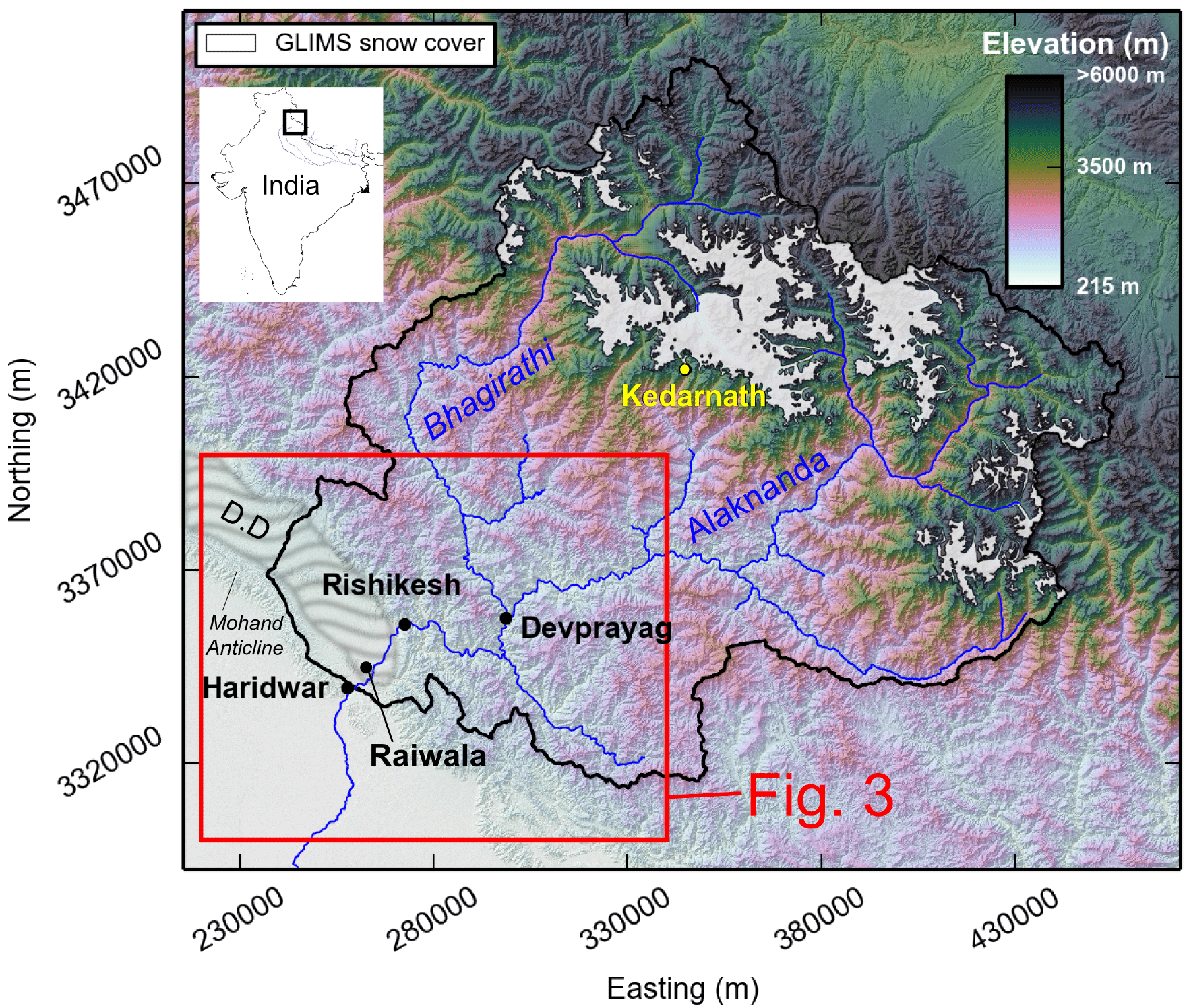
Figure 1 The 30 m Shuttle Radar Topography Mission (SRTM) digital elevation model (DEM) of the Ganga catchment. Coordinates are projected in Universal Transverse Mercator (UTM) zone 44N. Glacier coverage as documented in the Global Land Ice Measurements from Space (GLIMS) database is also shown in white. The red box represents the spatial area shown in more detail in Fig. 3. “D.D” refers to the Dehra Dun region which is delineated by the grey striped area.

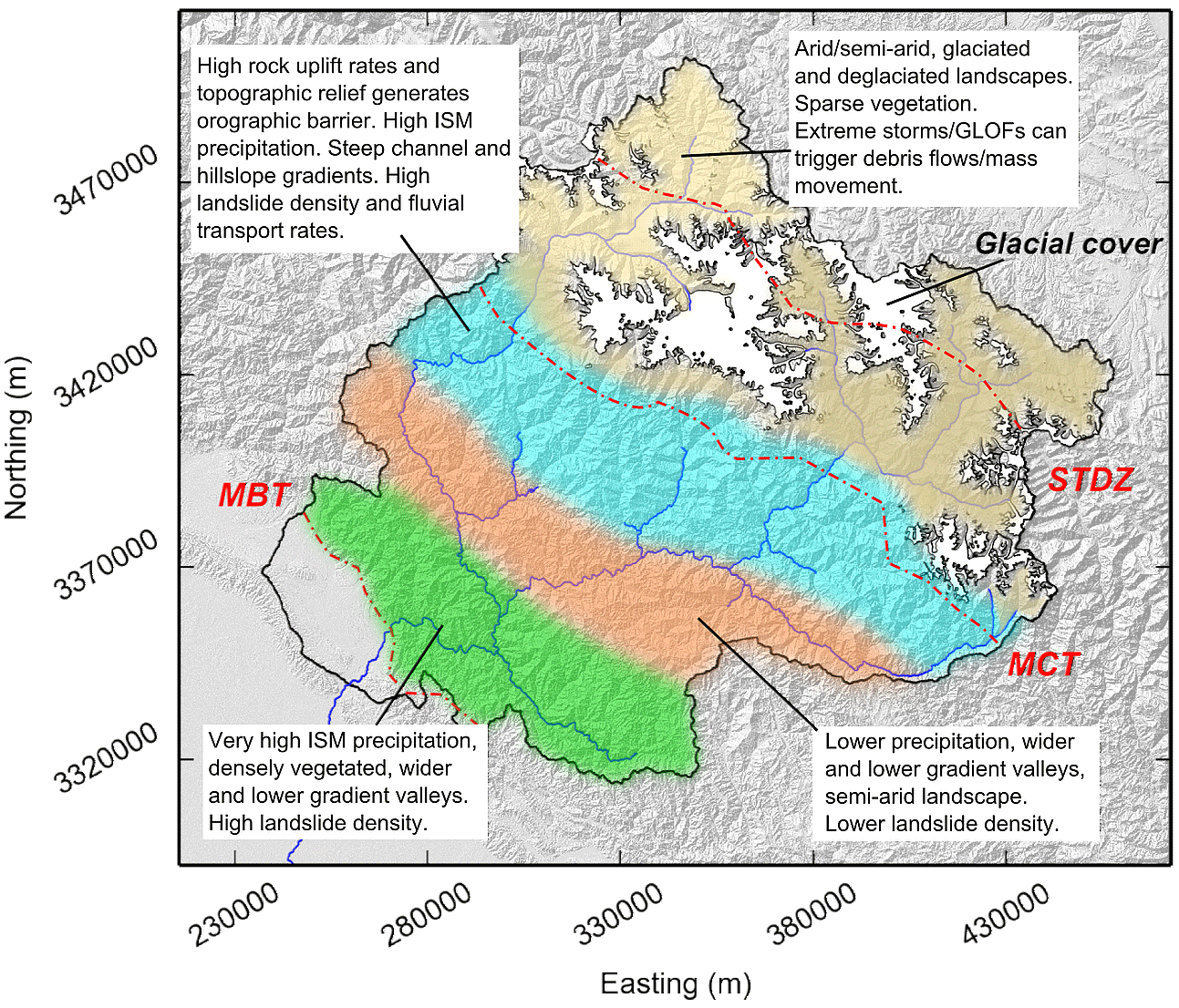
Figure 2 Broad distribution of geomorphic process domains across the Ganga catchment. The approximate positions of the Main Boundary Thrust (MBT), Main Central Thrust (MCT) and South Tibetan Detachment Zone (STDZ) are shown by red dashed lines following Ray and Srivastava (2010). Relative landslide density was determined by manual mapping of >400 landslides across the Ganga catchment using Google Earth imagery, where landslides in glacially influenced parts of the catchment were excluded. ISM denotes the Indian Summer Monsoon.

Sample information

A number of slack water and flood deposits in the Ganga valley record rapid sediment accumulation over the Ganga floodplain during high flow events in the late Holocene (Wasson et al., 2013). Seven of these flood units have been dated between ∼280 and 600 years old by OSL and calibrated with ¹⁴C ages from preserved charcoal fragments (Wasson et al., 2013). These deposits are preserved in a slightly wider part of the bedrock gorge upstream of the mountain front, where flood waters would have backed up as the river enters the narrower gorge immediately downstream. Additional deposits were studied by Wasson et al. (2013) at Devprayag and Raiwala (Fig. 1) although they recorded small flood couplets as opposed to single flood event deposits. Stacked sand–silt couplets representing phases of persistent flooding were also identified between 2500–1200 and 320–209 years BP at Devprayag and were attributed to changes in the spatial extent of the ISM based on geochemical evidence (Srivastava et al., 2008).

During 2013, heavy rainfall between the 15 and 17 June was centred over the Alaknanda and Bhagirathi catchments and generated significant flash flooding and numerous landslides, causing notable damage to the Kedarnath region in the Alaknanda catchment (Fig. 1). A moraine dammed lake (Chorabari) had formed northwest of the Kedarnath region in response to the elevated levels of snowmelt runoff in the preceding month, which is also understood to have burst on the morning of 17 June 2013, releasing water with a peak discharge estimated at 783 m³ s⁻¹ into the Alaknanda valley (Durga-Rao et al., 2014). Flash flooding is not an uncommon phenomenon in the Ganga basin; other large-magnitude events were documented in 1894 and 1970 (Rana et al., 2013). Both of these flood events were attributed to the breaching of dams created by landslides on the tributaries of the Alaknanda River, following unusually high rainfall events. Sediment deposited following the 2013 floods upstream of Devprayag (Fig. 1) over-topped the 1970 flood sediment deposits (thought to be the largest flood during the last 600 years), suggesting that the 2013 flood water levels were the highest in the Alaknanda valley during at least the last 600 years (Rana et al., 2013; Wasson et al., 2013), and possibly since the Last Glacial Maximum (Devrani et al., 2015). The 2013 event also presents a rare opportunity to resample ¹⁰Be concentrations following an extreme flood event in the modern Ganga River, to compare against pre-event concentrations as documented by Lupker et al. (2012).

3 Methods

3.1 Sample collection

Quartz-rich sand samples were taken from modern gravel bars (herein termed modern samples) and independently dated terrace and floodplain deposits (Fig. 3). ¹⁰Be concentrations measured from floodplain samples are thought to accurately reflect upstream basin-averaged denudation rates if sediment residence time in the floodplain is sufficiently short to avoid additional ¹⁰Be accumulation prior to burial (Gosse and Phillips, 2001; Lupker et al., 2012). In the instance of thick event beds (>2 m), sediment at the base of each bed is assumed to have been rapidly buried to a depth greater than the penetration range of cosmic rays, so it will have remained shielded since burial and therefore should have accumulated minimal post-depositional ¹⁰Be. In order to reduce the impact of ¹⁰Be accumulation after deposition of dated terraces, sediment samples were collected from the base of thick beds (>1 m) that record individual flood events either as overbank fines or as channel braid bars (Wasson et al., 2013). At least 2 kg of quartz-rich sand were sieved from the base of event beds. All samples were collected following horizontal digging for ∼1 m into steep cuts through the deposits to minimise post-burial ¹⁰Be production. ¹⁰Be concentrations from terrace and floodplain samples were corrected for post-depositional ¹⁰Be accumulation by considering that the samples had been exposed to cosmic radiation since deposition at the same depth as they were sampled from. For the slower, long-term sedimentation rates of ∼2 mm yr⁻¹ in the older early Holocene terraces, only samples from the base of very thick-bedded (>1–2 m) gravels were used to minimise post-depositional effects, where it is assumed that samples would have been largely shielded from further ¹⁰Be production. Sample depths and post-depositional corrections are presented in Table 1. Sand was taken from the base of several metre thick sand deposits (RFLO and DV2013) abandoned following the summer 2013 Alaknanda flood event to evaluate the degree of mixing of sand during a single extreme event.

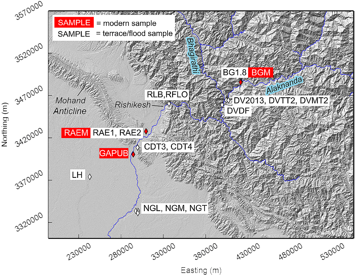
Figure 3 Modern (red) and terrace/floodplain/flood (white) sample locations and names in the lower Ganga catchment. See Table 1 for full description of samples.

Wasson et al. (2013)Srivastava et al. (2008)Ray and Srivastava (2010)Ray and Srivastava (2010)Sinha et al. (2010)Wasson et al. (2013)Wasson et al. (2013)Sinha et al. (2010)Sinha et al. (2010)Verma (2016)Sinha et al. (2010)Sinha et al. (2010)Sinha et al. (2010)

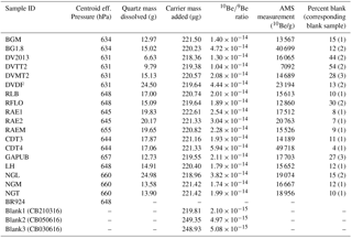
Table 1 ¹⁰Be sample details, ¹⁰Be concentrations and modelled erosion rates. Full sample details are given in Table A1.

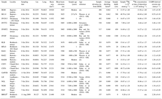
^a Average shielding factor is the average of the combined shielding factors: topographic, snow and self-shielding values. These were calculated using a depth-integrated approach (see Mudd et al., 2016).
^b Details for this sample (BR924) are from Table 1 in Lupker et al. (2012). We have recalculated the erosion rate using the Catchment-Averaged denudatIon Rates from cosmogenic Nuclides (CAIRN) method (Mudd et al., 2016).

3.2 Sample preparation and analysis

Floodplain, terrace and modern river sand samples were first dried before sieving into a number of grain size fractions. The main grain size fraction of interest in this study is 250–500 µm. Samples with sufficient material in the 250–500 µm fraction were then passed through a horizontal Frantz to remove magnetic minerals. Samples were also supplemented with material from the 125–250 µm grain size fraction where there was insufficient material in the 250–500 µm fraction. While previous studies have demonstrated that different sediment grain size fractions may be selectively enriched in ¹⁰Be (e.g. Puchol et al., 2014; Schildgen et al., 2016), analysis from Lupker et al. (2012) on the 125–250 and 250–400 µm grain size fractions (from the same sample) at the Himalayan mountain front reveal no systematic differences in ¹⁰Be concentration. Following this procedure, samples were put through repeated dissolutions in aqua regia and diluted hydrofluoric (HF) acid and HNO₃ solutions to remove mineral phases other than quartz. Quartz samples were then etched with HF to remove between 30 and 50 % of their volume. The purity of the clean quartz cores was then tested by inductively coupled plasma atomic emission spectroscopy (ICP-AES). All the Al concentrations in the quartz cores were below 300 ppm. Between 7 and 30 g of quartz cores were dissolved in concentrated HF. Samples were spiked with ∼220 µg of a ⁹Be carrier produced in the cosmogenic isotope analysis facility at the Scottish Universities Environmental Research Centre (SUERC) from phenakite crystals. The ¹⁰Be carrier concentration is $\sim \mathrm{9}\times {\mathrm{10}}^{-\mathrm{16}}$ ¹⁰Be∕⁹Be. A procedural blank was prepared together with each group of samples. Be was isolated from the solutions following routine column chemistry (Darvill et al., 2015). ¹⁰Be∕⁹Be ratios of the produced BeO targets were measured with the 5 MV Pelletron accelerator mass spectrometer (AMS) at SUERC (Xu et al., 2010). ¹⁰Be data were calibrated against the National Institute of Standards and Technology standard reference material (NIST SRM) 4325. The activity of NIST SRM 4325 corresponds to a nominal ¹⁰Be∕⁹Be ratio of $\mathrm{2.79}\times {\mathrm{10}}^{-\mathrm{11}}$ for a ¹⁰Be half-life of 1.36×10⁶ years. The processed blank ratios ranged between 4 and 54 % of the sample ¹⁰Be∕⁹Be ratios (see Table A1 for details). The uncertainty of this correction is included in the stated standard uncertainties.

3.3 Denudation rate calculations

Catchment-averaged denudation rates were calculated for each sample using the CAIRN (Catchment-Averaged denudatIon Rates from cosmogenic Nuclides) method (Mudd et al., 2016), which estimates production and shielding factors on a pixel-by-pixel basis, rather than a catchment-averaged shielding factor as in more commonly used CRN analysis packages such as CRONUS (Cosmic-Ray prOduced NUclide Systematics in Earth) (Balco et al., 2008). An average rock density of 2650 kg m⁻³ was used (the default for CAIRN). Snow shielding was determined for the Ganga catchment using data downloaded from the Global Land Ice Measurements from Space (GLIMS) glacier database (Armstrong et al., 2005); production rates beneath snow-covered areas were assumed to be zero. The GLIMS data suggest that ∼14 % of the Ganga catchment is glaciated (Fig. 1), which is ∼12 % higher than estimates in Lupker et al. (2012) which were produced prior to the completion of the GLIMS database in this region. The proportion of catchment glacier cover is likely to have been notably higher during the early Holocene, and as such, production rates may have been lower when averaged over the full catchment. We therefore consider the production and erosion rates calculated for ancient deposits as maximum values.

4 Results

The ¹⁰Be concentrations of the two modern samples near the mountain front (GAPUB and RAEM) are 17.70 and 15.53×10³ atoms g⁻¹, respectively. When combined with sample BR924 from Lupker et al. (2012) which was similarly collected near the mountain front, an average concentration of 14.1×10³ atoms g⁻¹ is estimated for modern samples. The concentration of modern sample BGM taken from further upstream of the Alaknanda–Bhagirathi confluence is 13.56×10³ atoms g⁻¹ which is comparable to the average modern concentration of samples close to the mountain front which integrates the full Bhagirathi catchment. ¹⁰Be concentrations of the majority of samples, both from ancient terraces and recent flood deposits, largely fall within the error of modern detrital samples (Fig. 4 and Table 1). Only three samples (BG1.8, DVDF and CDT4) display ¹⁰Be concentrations considerably greater than the upper error bound (19.1×10³ atoms g⁻¹) of modern river samples; the average concentrations of these terrace samples are in excess of 20×10³ atoms g⁻¹. Only one sample, DVTT2, has an average concentration (6.66×10³ atoms g⁻¹) notably below the lower error bound of the modern samples (8.20×10³ atoms g⁻¹). Samples taken from flood deposits associated with the 2013 Alaknanda flood (DV2013 and RFLO) reveal concentrations of 16.06 and 12.85×10³ atoms g⁻¹, respectively, which fall well within the error of modern river sediment samples.

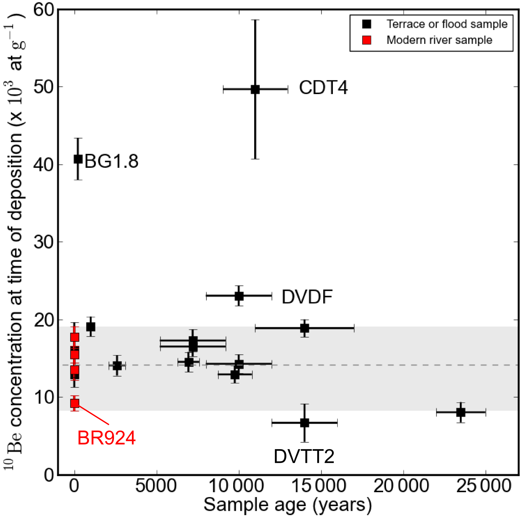
Figure 4 Measured modern river (red) and terrace or flood/floodplain (black) ¹⁰Be concentrations relative to their depositional age. Horizontal error bars represent the published age error associated with the independently dated deposit, and vertical error bars represent error in ¹⁰Be concentrations determined in this study. Sample BR924 from Lupker et al. (2012) is also included and labelled.

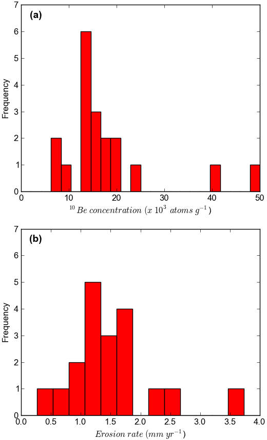
In a frequency histogram of ¹⁰Be concentration data (Fig. 5a), the three samples with the highest concentrations (BG1.8, DVDF and CDT4) produce a positively skewed distribution. These samples represent a fine-grained ∼300-year flood deposit (Wasson et al., 2013), ∼10 000-year old terrace fill (Srivastava et al., 2008) and ∼11 000-year old terrace fill (Sinha et al., 2010), respectively (see Table A1 for further sample details). With the removal of samples BG1.8 and CDT4 from the frequency histogram, the ¹⁰Be concentration data generate a near-normal distribution (Fig. 5a).

Results from CAIRN modelling of all concentrations suggest that catchment-averaged denudation rates for each sample largely lie within the variability of modern detrital samples (Fig. 5b). Based on the measured concentrations, these samples correspond to integration timescales of ∼500 years, representing the average time period when the erosion rate is considered to be constant, based on the time needed to erode one mean attenuation path length (approximately 60 cm/erosion rate) (Lal, 1991). There does not appear to be a spatial trend between ¹⁰Be concentration and upstream catchment area, even downstream of large tributary confluences (Fig. 6). The impact of high ¹⁰Be concentration samples on the frequency histogram of erosion rates calculated using CAIRN modelling is less apparent (Fig. 5b), but the distribution shows significant spread. Calculating sediment flux estimates from a single erosion rate at the upper end of the distribution could result in sediment flux estimate being up to 7 times larger than one based on a sample at the lower end of the distribution.

Figure 5 (a) Frequency histogram of mean ¹⁰Be concentrations shown in Fig. 4. (b) Frequency histogram of mean erosion rates calculated using the CAIRN method.

5 Impact of stochastic inputs on ¹⁰Be variability and sediment flux estimates

5.1 CRN sample interpretation

Possible explanations for the high-concentration measurement at BG1.8 may include insufficient shielding since deposition, resulting in ¹⁰Be enrichment of the deposit. Unlike other samples analysed here, the event bed associated with this sample was only ∼0.5 m thick so burial (and therefore complete shielding) was unlikely to be instantaneous. Whilst a number of additional samples were taken from this exposure to try and produce depth-concentration profiles, their grain size was too fine for ¹⁰Be analysis. However, the maximum ¹⁰Be enrichment at the site during burial is likely to only be ∼1650 atoms g⁻¹ based on local CRN production rates and sample depth, which is less than the measurement uncertainty. With respect to the two terrace deposits (DVDF and CDT4), high concentrations could also have been produced if the samples were overwhelmed by locally derived, high-concentration hillslope sediment which was not well mixed. Samples with the largest ¹⁰Be concentration variability also seem to focus around 10–15 ka (Fig. 4), which may represent a period of post-glacial conditions where a combination of low ¹⁰Be concentration material (generated by glacial erosion) and high ¹⁰Be concentration sediment (due to lower precipitation rates and therefore slower erosion of non-glaciated landscapes) generated during the Last Glacial Maximum may have been mobilised as the ISM intensified during the early Holocene.

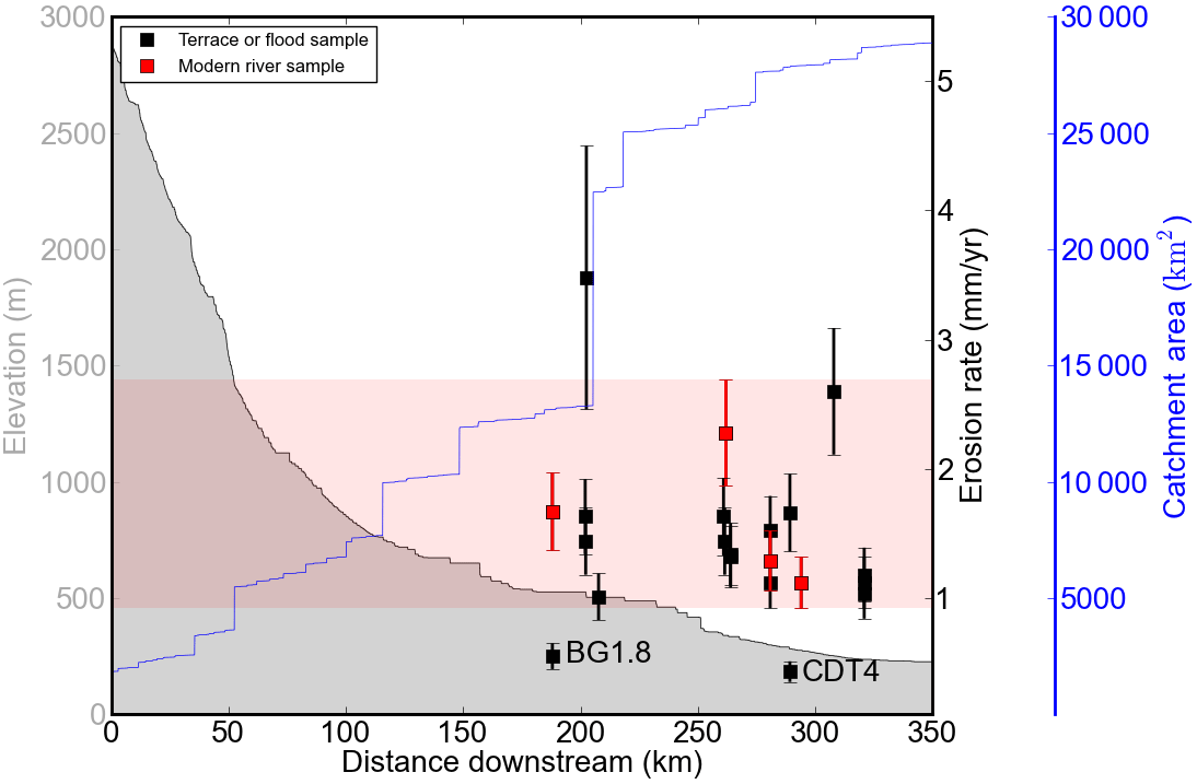
Figure 6 Modern river (red) and terrace or flood/floodplain (black) catchment-averaged erosion rates with respect to distance downstream, sample elevation (grey shaded region) and upstream catchment area (blue line). Vertical error bars represent error associated with the modelled erosion rate and propagated ¹⁰Be concentration errors used to derive the erosion rate. The red shaded area represents erosion rates within the error of modern samples. Outliers BG1.8 and CDT4 are labelled.

5.2 Impact of landslides on ¹⁰Be variability

A range of processes are likely to drive temporal variability in ¹⁰Be concentrations in sand sampled close to the outlet of large Himalayan catchments. The most obvious process is stochastic inputs generated by mass wasting of hillslopes, which generates large quantities of sediment with relatively low ¹⁰Be concentrations. Frequency histograms presented in Fig. 5 suggest that such stochastic processes may form part of the natural background variability, as low-concentration values tend not to skew the distributions. More samples would be needed to draw a clearer picture on this. Below, we examine how different erosional processes may drive the types of temporal variability in ¹⁰Be concentrations measured close to the Ganga outlet. This is approached using a numerical analysis of catchment-averaged ¹⁰Be concentrations derived under varying background erosion rates, landslide depth, surface ¹⁰Be production rates and degrees of event buffering (i.e. varying proportions of “event” sediments are mixed into the fluvial network). Given the complexity of this type of landscape (e.g. multiple geomorphic process domains, climatic variability), we do not attempt to mimic these processes and reproduce measured concentrations or erosion rates (e.g. Niemi et al., 2005), nor do we use this analysis to determine the relative contributions required from stochastic processes (e.g. area and depth of landsliding) to produce our observed concentrations. Instead, this numerical analysis is used to explore the sensitivity of outlet ¹⁰Be concentrations to a range of parameters and scenarios that may drive variability. The analysis considers the impact of a single sediment-generating event, as opposed to the evolution of catchment-averaged concentrations which occur in response to a distribution of landslides occurring over timescales of hundreds to thousands of years across a landscape (e.g. Niemi et al., 2005; Yanites et al., 2009).

The relative ¹⁰Be contribution by landsliding can be approximated to first order by calculating the volume of material generated by the event and the average concentration of that material. The concentration of landslide material is strongly controlled by the local surface ¹⁰Be production rate and depth of the landslide. ¹⁰Be production rates rapidly diminish in the upper few metres of the Earth's surface (Lal, 1991; Niedermann, 2002; Stone, 2000) following

$$\begin{array}{}\text{(1)}& P\left(z\right)=P_{\mathrm{0}}{e}^{\left(\frac{-z\mathit{\rho }}{\mathrm{\Lambda }}\right)},\end{array}$$

where z is the depth below the surface (cm), Λ is the attenuation length (g cm⁻²), ρ is rock density (g cm⁻³), and P₀ is the surface nuclide production rate (atoms g⁻¹ yr⁻¹). At depths greater than ∼2 m the CRN production rate (by spallation reactions) is negligible, as is muon production, as atoms generated by muon interactions represents a small proportion relative to those produced by spallation reactions in the upper 1–2 m of the Earth's surface (e.g. Niedermann, 2002). Here, we calculate the average concentration of landslide material by integrating the surface production rate within the upper 2 m; we find that the depth-averaged production rate of the upper 2 m (P_d) is ∼30 % of P₀. This was converted into a ¹⁰Be concentration (C) in atoms g⁻¹ using

$$\begin{array}{}\text{(2)}& C={\displaystyle \frac{\left(P_{\mathrm{d}}\mathrm{\Lambda }\right)}{\mathit{\rho }\left(\mathit{ϵ}+\mathrm{\Lambda }\mathit{\lambda }/\mathit{\rho }\right)}},\end{array}$$

from Niedermann (2002), where we assume that the ¹⁰Be decay constant (λ) is equal to 0 over the timescales we are concerned with (<10³ years) relative to the half-life of ¹⁰Be. We use ρ=2.7 g cm⁻³ and Λ=160 g cm⁻². We also assume a steady-state erosion rate (ϵ) across the upstream catchment. For landslide depths of less than 2 m, the average concentration was calculated based on the production rate integral specific to that depth. For simplicity, we initially assume that the rest of the catchment is eroding uniformly at a background erosion rate, with a catchment average ¹⁰Be production rate of 35 atoms g⁻¹ yr⁻¹ which is comparable to the catchment-averaged production rate calculated for the Ganga catchment in CAIRN. The concentrations calculated at the Ganga outlet also assume complete sediment mixing. The ¹⁰Be concentration at the catchment outlet (α_{event + uniform}) is then calculated using

$$\begin{array}{}\text{(3)}& {\mathit{\alpha }}_{\mathrm{event}+\mathrm{uniform}}={\displaystyle \frac{\left({\mathit{\alpha }}_{\mathrm{uniform}}{\mathit{\varphi }}_{\mathrm{uniform}}\right)+\left({\mathit{\alpha }}_{\mathrm{event}}{\mathit{\varphi }}_{\mathrm{event}}\right)}{{\mathit{\varphi }}_{\mathrm{uniform}}+{\mathit{\varphi }}_{\mathrm{event}}}},\end{array}$$

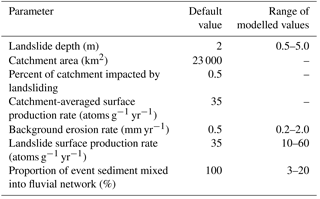
where ϕ_uniform and α_uniform are the background sediment flux and ¹⁰Be concentration, respectively. ϕ_event and α_event are the event- or landslide-generated sediment flux and ¹⁰Be concentration, respectively. A series of sub-catchments was then selected to examine the influence of spatial variability in surface production rates across the Ganga basin, to provide a realistic range of values in the numerical analysis (Fig. 7). Average shielding factors (snow and topographic shielding) were first calculated for each of these sub-catchments using the CAIRN method (Mudd et al., 2016), which were then used in the online CRONUS v2.3 calculator (Balco et al., 2008) to calculate production rates, using a constant production rate model with a Lal–Stone scaling scheme for spallation (Fig. 7 and Table 2). The default landslide surface production rates were initially set to the same as the catchment-averaged production rate. The landslide surface production rates were then varied based on realistic production rates derived from sub-catchments across the Ganga catchment (Table 2). Earthquake-induced landsliding datasets from the 1999 Chi-Chi (Taiwan) and 2015 Gorkha (Himalaya) earthquakes (Lin and Tung, 2004; Martha et al., 2017; Roback et al., 2018) state that the total landslide areas were ∼128 and 87–90 km², respectively. Areas of these sizes represent approximately 0.5 % of the Ganga catchment area. We therefore use the value of 0.5 % as an approximation of the proportion of the hypothetical catchment to have been impacted by landsliding. In the analysis, the average depth of the landslides was varied from 0.5 to 5 m, the average background erosion rate from 0.2 to 2.0 mm yr⁻¹ and the average landslide surface production rate from 10 to 60 atoms g⁻¹ yr⁻¹. We use an average landslide depth where, in reality, the depths of individual landslides occurring in response to an earthquake or intense storm are likely to fit a power–law distribution (Hovius et al., 1997). However, at any point in time it is unlikely that the full power–law distribution of landslide depths is sampled or integrated into the catchment wide signal, due to the recurrence interval and amount of time taken to evacuate larger and deeper co-seismic landslides. Sediment generated by inter-seismic landsliding is assumed to be represented in the background erosion rate imposed across the catchment, whilst the sediment generated by the landslide event is assumed to reflect a large co-seismic event (i.e. the tail-end of landslide frequency distribution). We also assume that the ¹⁰Be concentration profile in the upper 2 m of the landscape is in steady state before landsliding. This assumption is more important in slowly eroding landscapes, where it may take tens of thousands of years to reach secular equilibrium (Dunai, 2010). This may result in over-estimated landslide ¹⁰Be concentrations in our analysis, if the ¹⁰Be concentration profile is not in equilibrium. Similarly, landsliding is more likely to occur in parts of the landscape undergoing faster erosion rates where, above a certain hillslope gradient, erosion rate becomes less closely correlated (to hillslope gradient) as the main mechanism of erosion changes from transport-limited to detachment-limited processes (Binnie et al., 2007). It might therefore be expected that these regions have initially lower ¹⁰Be concentrations. By increasing the average landslide erosion rate (relative to the catchment-average erosion rate applied across the rest of the catchment) in our analysis, we indirectly assess the importance of such effects.

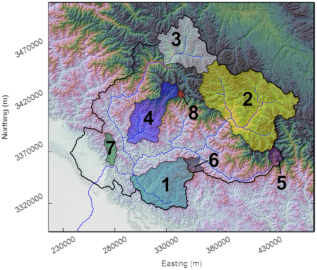
Figure 7 Location of sub-catchments used to determine the variability in production rate across the Ganga catchment (presented in Table 2).

Table 2 Catchment area, mean catchment elevation and average ¹⁰Be surface production rate for sub-catchments in the Ganga catchment.

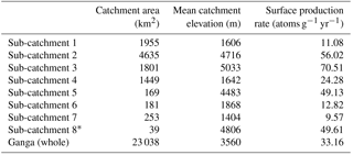
^∗ This sub-catchment represents the area upstream of Kedarnath during the 2013 Alaknanda flooding.

We calculate “volumetric sediment flux” by combining the flux derived from background erosion rates with the calculated landslide flux and compared these to sediment flux estimates derived from the ¹⁰Be concentration at the catchment outlet (which we term the “CRN-derived sediment flux”). For a catchment eroding at a uniform rate (ϵ in mm yr⁻¹), the CRN-derived sediment flux is the product of the erosion rate, catchment area (A in km²) and average rock density (ρ in kg m⁻³).

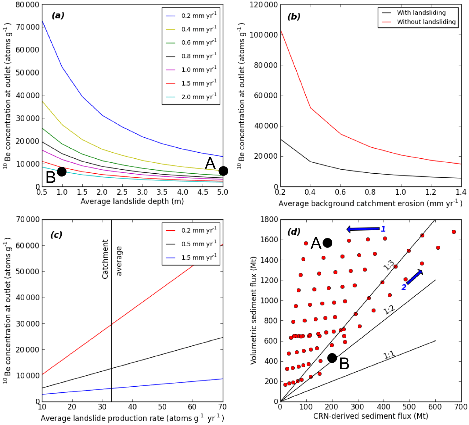
Figure 8 (a) Variations in ¹⁰Be concentration predicted at the outlet in response to increasing landslide depth and as a function of background erosion rates (represented by coloured lines). (b) Outlet ¹⁰Be concentration as a function of background erosion rate (where all other parameters are constant at default values – see Table 3), for a system undergoing no landsliding (red line – where erosion is driven purely by background erosion) and another with 2 m deep landsliding over 0.5 % of the catchment area (black line). (c) Outlet ¹⁰Be concentration under varying average landslide ¹⁰Be surface production rates (based on Table 2) and background erosion rates (coloured lines). The black vertical line represents the whole Ganga-catchment-averaged production rate of ∼33 atoms g⁻¹ yr⁻¹. (d) Comparison of volumetric and CRN-derived sediment fluxes from analysis in panels (a)–(c). The blue arrow labelled 1 shows the effect of decreasing background erosion rate, and the blue arrow labelled 2 shows the effect of increasing landslide depth and/or landslide ¹⁰Be production rate. The black dots in panels (a) and (d) represent scenarios A and B which are discussed in more detail later and in Fig. 13.

In this analysis, we assume that sediment storage between the region affected by landslides and the outlet is small relative to the total sediment flux of the catchment. Unlike the eastern and western Himalaya, the central Himalaya (which is largely drained by tributaries of the Ganga River) is comparatively void of large valley fills (Blöthe and Korup, 2013), which is likely to limit large volumes of sediment storage and sediment residence times. Recent modelling has also suggested that approximately 50 % of coarse material generated by post-seismic landsliding is evacuated within 5 to 25 years (Croissant et al., 2017). In our scenarios, we initially assume complete evacuation of material to the outlet within a year. We then run additional analysis where much smaller proportions of the event material are mixed into the fluvial network in this first year (3, 5, 10 and 20 % of the event sediment). The default and range of values tested for each parameter in the analysis are shown in Table 3.

Based on the above calculations, our results suggest that increasing the average landslide depth results in a marked decrease in outlet ¹⁰Be concentration, most notably between depths of 0.5 and 3 m (Fig. 8a). This can be explained through the exponential decay in ¹⁰Be production rates in the upper 2 m of the landslide (Lal, 1991; Niedermann, 2002; Stone, 2000). This reduction in concentration is greatest under lower background erosion rates. Increasing background erosion rates from 0.2 to 2.0 mm yr⁻¹ also reduces the effect of landsliding on outlet ¹⁰Be concentrations (Fig. 3b). Under lower background erosion rate, landslide material represents a greater proportion of the total sediment flux, so the system has less capacity to buffer the landslide input and the ¹⁰Be concentration is more sensitive to deeper landslides. We also find that outlet ¹⁰Be concentrations are sensitive to the average landslide surface production rate. Where the average surface production rate of the landsliding is increased (e.g. comparable to that expected in high-altitude sub-catchments of the Ganga – see Table 2), predicted outlet ¹⁰Be concentrations also increase relative to scenarios with otherwise identical parameter values (Fig. 8c). Interestingly, we also find that volumetric sediment flux estimates are consistently higher than CRN-derived fluxes (Fig. 8d). Increasing background erosion rates increases both CRN-derived and volumetric sediment flux estimates, but increasing average landslide depth or landslide ¹⁰Be production rate can reduce CRN-derived sediment flux estimates to a much greater degree than volumetric flux estimates.

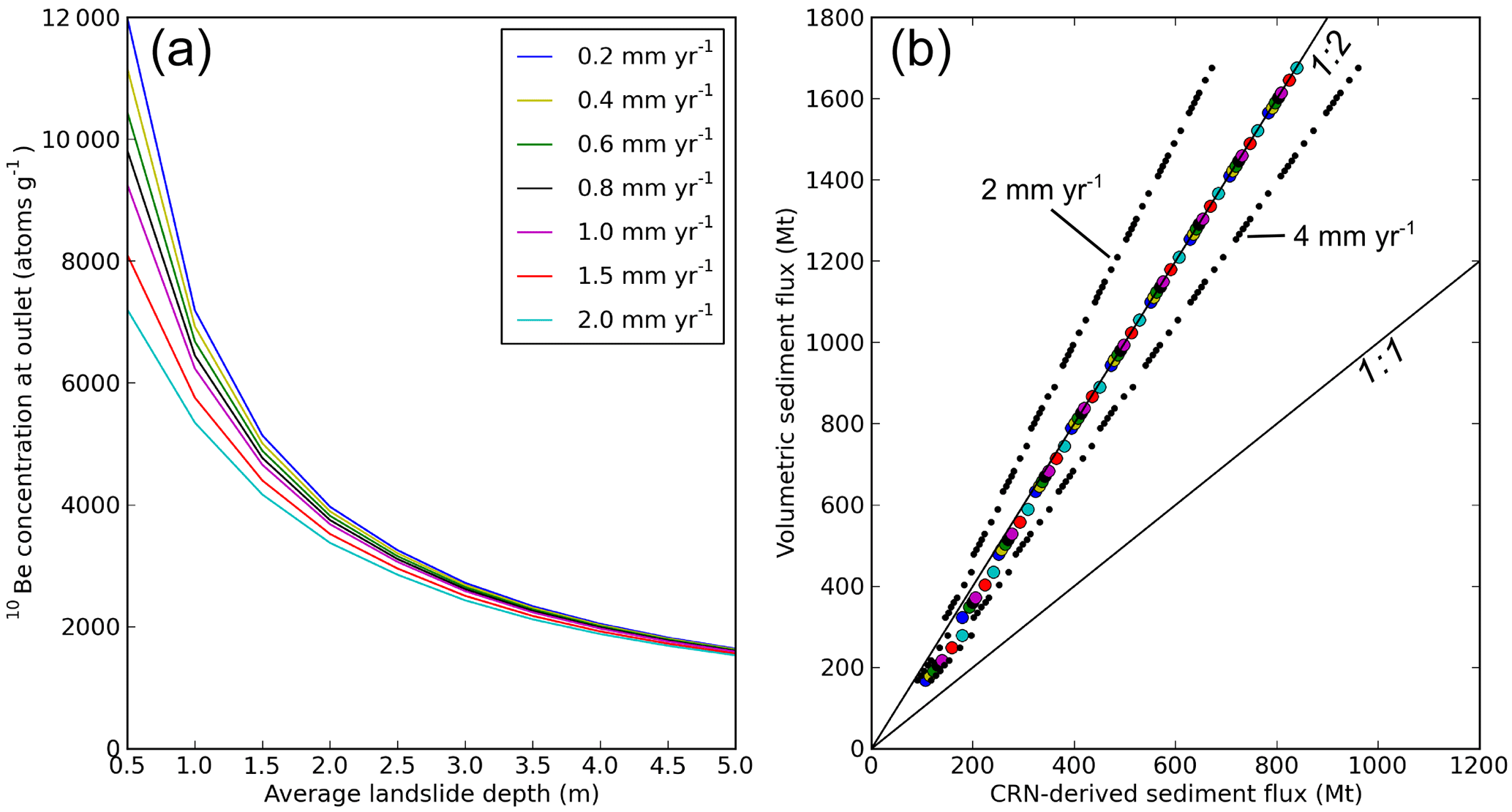
Figure 9 (a) Effect of increasing average landslide erosion rate to 3.0 mm yr⁻¹on outlet ¹⁰Be concentrations in response to varying landslide depths and catchment background erosion rates. The overall range in outlet concentrations is notably lower than in Fig. 8a. Increasing the catchment-averaged erosion rate only has an impact on outlet concentrations where the input of landslide material is smaller, suggesting that the outlet concentration is dominated by landslide-derived material. (b) Comparison of volumetric and CRN-derived sediment fluxes for the same model conditions, where marker colour corresponds to background erosion rate shown in panel (a). The difference in volumetric and CRN-derived fluxes is much less than scenarios shown in Fig. 8d. In general, the volumetric flux is approximately double the CRN-derived sediment flux. By increasing and decreasing the average landslide erosion rate to 4.0 and 2.0 mm yr⁻¹ as shown by the smaller black markers, this relationship varies slightly.

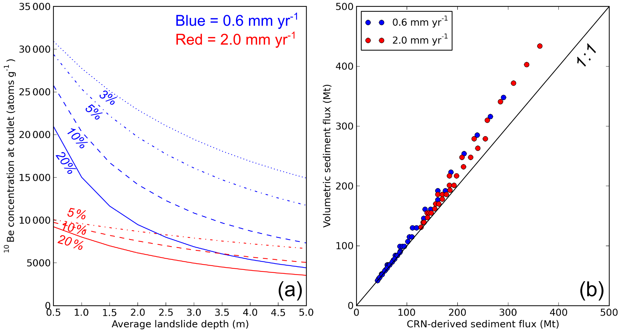
Figure 10 (a) Effect of event buffering on outlet ¹⁰Be concentrations, where smaller fractions (3, 5, 10 and 20 %) of the event sediment are mixed into the fluvial network based on two background erosion rates of 0.6 and 2.0 mm yr⁻¹ shown in blue and red, respectively. The event proportions are represented by the different dashed lines. The average landslide surface erosion rate is set to 3.0 mm yr⁻¹. Under faster background erosion rates, the effect of larger landsliding events is more easily buffered in outlet ¹⁰Be concentrations. (b) Comparison of volumetric and CRN-derived sediment fluxes for event buffering scenarios. Under these conditions, volumetric and CRN-derived sediment flux estimates are much more comparable. As the amount of landslide-derived material mixed into the system increases, volumetric sediment fluxes become slightly larger than CRN-derived sediment fluxes.

Table 3 Default and range of parameter values used in numerical analysis.

The average landslide erosion rate was increased to 3.0 mm yr⁻¹, based on estimates in Niemi et al. (2005), to mimic the effects of faster erosion rates in regions more prone to landsliding and landscapes without steady-state concentration profiles. Niemi et al. (2005) ran a series of numerical modelling scenarios to explore the ratio of landslide to bedrock weathering (background) erosion rates needed to reproduce measured CRN erosion rates in the Khudi catchment in Nepal. The best fit model runs were found to have landslide erosion rates of 3.35 mm yr⁻¹. By applying a comparable value of 3.0 mm yr⁻¹ to our calculations, a reduction in the absolute values and range of outlet ¹⁰Be concentrations is produced. The initial maximum outlet concentration of ∼70 000 (in Fig. 8a) is reduced to 12 000 atoms g⁻¹ under the lowest background erosion rate scenarios (Fig. 9a). This range of outlet ¹⁰Be variability is more comparable to that observed at the Ganga outlet, although outlet concentrations appear less sensitive to background erosion rates applied across the rest of the catchment. Furthermore, the difference in volumetric and CRN-derived sediment fluxes is also reduced (Fig. 9b). By reducing the proportion of event sediment mixed into the fluvial network, similar reductions in the amount of ¹⁰Be concentration variability generated at the outlet are also observed (Fig. 10a), and outlet concentrations are more sensitive to changes in catchment background erosion rates. Under faster background erosion rates (2.0 mm yr⁻¹), the variability generated by events of all depths can be effectively masked by background variability where only 10 % of the event sediment is mixed in (i.e. such that the outlet concentration lies within 100 % of the maximum value). Similarly, under lower background erosion rates of 0.6 mm yr⁻¹, the fraction of event sediment needed to generate variability within 100 % of the highest concentration is slightly lower at 3 %.

Our analysis generates variability in ¹⁰Be concentrations that is considerably larger than what we document in the Ganga catchment (Fig. 4), suggesting that buffering of stochastic inputs must occur (Croissant et al., 2017). The evacuation time of fine-grained sediment (sand and finer) is likely to be fast relative to the coarse fraction, as the fine-grained fraction is annually entrained and transported downstream during months impacted by the ISM. This is supported by grain size analysis (Dingle et al., 2016) along a number of exposed gravel bars within the Ganga catchment, which demonstrate that the channel bed is comprised largely of grain sizes >1 mm, even beneath the surface armour layer. Typically, grain sizes <1 mm represent less than ∼15 % of the grain size distribution (Fig. 11) which is also observed across other catchments of the Ganga River. This suggests that there is relatively little in-channel storage (or mixing) of finer grained sediments relative to the large fluxes of these river systems, which on entering the Ganga Plain, are thought to be largely dominated (>90 %) by sand-sized (and finer) sediments (Dingle et al., 2017). However, the majority of landslide deposits are likely to be made of coarser material (Attal and Lavé, 2006; Attal et al., 2015) which will take longer to be evacuated or abraded into smaller and more easily transportable grain sizes. Whilst landsliding may generate the quantities and ¹⁰Be concentrations of sediment required to drive significant changes in concentration at the outlet, the evacuation timescales of these event sediments buffers their impact. Evacuation of event deposits over decadal to centennial timescales will reduce the ratio of background to event sediment fluxes (Croissant et al., 2017) and likely limit the impact on ¹⁰Be concentrations documented at the outlet.

5.3 Other potential sources of variability in ¹⁰Be concentration

Whilst landsliding with different depths and from different parts of the Ganga catchment is likely to represent a key component in ¹⁰Be variability, a number of other factors may also contribute, which are discussed below. Firstly, spatially variable distributions of quartz-rich lithologies across the Ganga catchment may lead to over- and under-estimation of denudation rates in specific lithological settings. However, potential variations in sediment quartz content have been assessed by Vance et al. (2003) in the Ganga catchment, who concluded that the correction due to the dilution of quartz from sediments sourced from carbonate-rich series in the catchment is of a similar magnitude (maximum of ∼9 % change in erosion rate for sub-catchments in the High Himalaya) to the production rate estimates and analytical errors. Recent studies have also highlighted the effect of grain-size-dependent ¹⁰Be enrichment, where coarser gravel-sized fractions have been documented to yield higher apparent denudation rates than the medium sand-sized fraction which is typically sampled (Lukens et al., 2016; Puchol et al., 2014; Schildgen et al., 2016) as a result of the process through which the different grain size fractions are generated (e.g. reworked hillslope material, landsliding), or differing sediment source elevations. Similarly, downstream lags in ¹⁰Be denudation rate spikes have been observed along the Tsangpo–Brahmaputra River in the eastern Himalayan syntax (Lupker et al., 2017), due to the distance which sediment generated in the rapidly uplifting Namcha Barwa – Gyala Peri massif must travel before being abraded into the grain size fraction used for sampling. However, modern samples collected close to the Ganga outlet are not likely to be influenced by either process, as the majority of sediment has already been abraded into sand by this point (Dingle et al., 2017). Similarly, a number of the floodplain and terrace deposits sampled were entirely sand. Exceptions to this include terrace deposits CDT3, CDT4, DVDF, DVMT2, DVTT2 and RLB, where sand samples were taken from poorly consolidated fluvial deposits containing imbricated and well-rounded quartzite cobbles and pebbles. However, additional ¹⁰Be samples were not run on individual clasts in these deposits to determine whether the coarser fraction yielded higher apparent denudation rates.

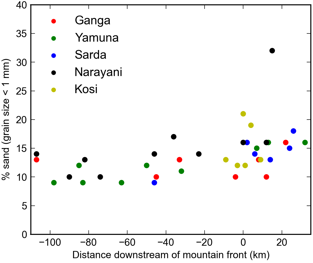
Figure 11 Volumetric sand (grain size <1 mm) proportions in sub-surface sediment samples along major tributaries of the Ganga River from Dingle et al. (2016).

Glacial lake outburst floods (GLOFs) are not uncommon across the Himalaya (e.g. Cenderelli and Wohl, 2003; Kattelmann, 2003) and have the potential to generate and mobilise large quantities of sediment. Geomorphic analysis following the 1977 and 1985 GLOFs in the Mount Everest region (Cenderelli and Wohl, 2003) suggested that much of the sediment eroded from the upper 10–16 km of the GLOF route was unconsolidated sediment (glacial till, colluvium, glaciofluvial terraces). Erosion was typically found to be limited in valleys with resistant bedrock or consolidated side walls. Similarly, the availability of unconsolidated material is also thought to be a key limiting factor in the volume of debris flows triggered following GLOFs, which can limit the erosive potential of the flow (Breien et al., 2008). In the absence of existing studies which document ¹⁰Be concentrations in proglacial lake sediments, we cannot infer how sediment released from the glacial lake may contribute to downstream variations in ¹⁰Be concentration. Geomorphological evidence in reaches downstream of GLOFs suggests that much of the sediment eroded by the flood is largely unconsolidated (glacially influenced) material from relatively shallow depths (<3 m; Cenderelli and Wohl, 2003) which is likely to have a complex exposure history. Given the relatively short length of the reach impacted downstream of the GLOF (relative to the full length of a system such as the Ganga), and the likely ¹⁰Be-enriched nature of surface deposits reworked by GLOFs, it seems unlikely that these types of events drive significant change in outlet ¹⁰Be concentrations. This is supported by work in the Marshyangdi River catchment in Nepal, which suggested that localised erosion in the upper glaciated catchment is almost an order of magnitude lower than fluvial incision rates in the upper Marshyangdi River (Heimsath and McGlynn, 2008). An analysis of the evolution of detrital ¹⁰Be concentrations along the Marshyangdi River suggested that low-concentration ¹⁰Be inputs from glaciated tributaries dilute main stem ¹⁰Be concentrations (Godard et al., 2012). In this instance, glacial erosion was averaged at ∼5 mm yr⁻¹ in the High and Tethyan Himalayan portions of the catchment, suggesting that glacially derived sediments may complicate detrital ¹⁰Be concentrations and interpretation of catchment-averaged denudation rates.

Extreme monsoonal storms, such as the one that generated the 2013 Alaknanda flooding, also have the potential to generate ¹⁰Be variability if hillslope runoff mobilises large quantities of unconsolidated sediment on valley sides and initiates mass wasting of hillslopes (Devrani et al., 2015; Dobhal et al., 2013). Sample DV2013 was collected from a thick sand unit at the Ganga channel margins (∼18 m above the modern channel) near Devprayag, known locally to have been deposited following the 2013 Alaknanda flood. We find that the ¹⁰Be concentration of this deposit (16.06×10³ atoms g⁻¹) also lies within the error of modern samples at the outlet. One interpretation is that the sediment generated by this event was sufficiently well mixed: upon reaching the Ganga outlet, it had minimal impact on the outlet ¹⁰Be concentration. Material mobilised by the Alaknanda flooding was largely unconsolidated, surficial hillslope material (Dobhal et al., 2013). As such, the ¹⁰Be concentration of these sediments will reflect their local production rate (∼50 atoms g⁻¹ yr⁻¹ – see Table 2) and background erosion rate. If erosion in the Alaknanda valley is driven primarily by large storm and flood events, unconsolidated surface sediments could have been accumulating ¹⁰Be since as early as the Last Glacial Maximum (LGM) (Devrani et al., 2015), with very low background erosion rates. As such, this type of erosive event may have generated sediment with a higher-than-expected ¹⁰Be concentration (given the depth of material removed) as a result of this ¹⁰Be-enriched surface layer.

Annual monsoonal storms may also contribute to the observed variability where storms tap into localised parts of the catchment. The hillslope sediments and reworked deposits these storms mobilise could vary in ¹⁰Be concentration in the different geomorphic process domains, as they will have variable ¹⁰Be production rates (which is a function of elevation), background erosion rates and deposit characteristics (e.g. deep-seated landslide). Background erosion rates in particular are likely to vary dramatically across the Ganga catchment as a result of spatially variable rock uplift, lithology, rainfall and vegetation cover (Anders et al., 2006; Bookhagen and Burbank, 2006; Vance et al., 2003). Earthquake-induced landsliding, GLOFs and extreme storm events are all likely to generate large quantities of sediment with ¹⁰Be concentrations that would be sufficient to drive significant change in the ¹⁰Be concentration recorded at the Ganga outlet. However, the impact that these processes have is limited by the ability of the river to entrain and transport this sediment out of the catchment. The evacuation timescales of sediment generated by these processes will likely vary as a function of the frequency and magnitude of localised storm events which mobilise mass-flow deposits from hillslopes into rivers sediment.

If this sediment is sourced close to the sampling location, it is also unlikely to be fully homogenised. The distance required to fully mix localised hillslope or tributary inputs has been shown to be as much as several kilometres (Binnie et al., 2006), which may induce variability in ¹⁰Be concentrations recorded at the outlet. In terms of modern river samples, a number of small ephemeral streams drain directly in the main Ganga channel near the outlet. During the monsoon season when these channels are active, sediment of differing ¹⁰Be concentrations will be transported to the main channel and may not be sufficiently mixed on reaching the outlet sampling locations. High-concentration samples documented close to the Ganga outlet could therefore represent locally derived and poorly mixed sediments, which reflect the erosional processes specific to a small frontal region of the catchment.

5.4 Suitability of ¹⁰Be as a proxy for sediment flux in large catchments

Our analysis of outlet ¹⁰Be concentrations suggests that the observed doubling in sediment delivery to the Bengal fan during the early Holocene may have been masked by the natural variability in palaeo-erosion rate or ¹⁰Be concentration data preserved close to the Himalayan mountain front. Whilst changes in the amount of sediment being delivered into the fluvial network may have occurred, the natural variability in ¹⁰Be concentrations delivered to the mountain front is sufficiently high that a doubling in volumetric flux (and therefore catchment-averaged erosion rate) cannot be clearly identified using detrital sampling. This is consistent with previous work using repeat ¹⁰Be samples from tectonically active watersheds in China, where it was concluded that replicability of data in these types of landscapes is likely to be poor, and that larger sample populations are needed to better represent upstream denudation rates (Gonzalez et al., 2017). Results from our study also support this finding, where we demonstrate that multiple samples are required to better characterise the temporal variability in ¹⁰Be concentrations at the Himalayan mountain front.

Using the approximate range of concentrations documented at the Ganga outlet (5000–30 000 atoms g⁻¹) as an example of natural variability, we can statistically constrain the number of samples required to capture this variability with repeat sampling. We proceed as follows: we produce a population of concentrations by choosing, at random, x values from a Gaussian distribution with a mean of 17 500 atoms g⁻¹ and a standard deviation of 4000 atoms g⁻¹, based on the values from the Ganga River samples. We repeat this procedure 100 times for each value of x, with x (the number of samples in a population) varying between 3 and 50. If we assume that the standard deviation of the concentrations for each population is a proxy for concentration variability within a set of samples, then the mean standard deviation of the 100 populations for a given number of samples x, and the standard deviation around this mean, give an indication as to whether the variability is well constrained. This is exemplified in Fig. 12: with increasing number of samples x within a population, the mean standard deviation increases and converges asymptotically towards the true value of 4000 atoms g⁻¹.

The standard deviation around the mean for the 100 populations generated for each number of samples x (error bars on the figure) reduces with increasing sample number; i.e. the variability becomes better constrained. With 18 samples, the mean standard deviation is within 10 % of the true standard deviation; more importantly, increasing the number of samples beyond 18 leads to minimal improvement, with the mean increasing by less than 0.3 % per additional sample. We therefore suggest that 18 samples represent a good balance between cost and performance when trying to characterise the natural ¹⁰Be concentration variability of a river system similar to the Ganga River. It is important however to note that the error bars around the mean standard deviation are large. Even with 50 samples, 68 % of the concentration populations (within 1 standard deviation of the mean assuming a Gaussian distribution of values – error bars in figure) will have a standard deviation within 23 % of the true value (in the range ∼3100–4500 atoms g⁻¹); nearly a third of the populations will therefore have a standard deviation beyond this bound. This figure is 35 and 44 % for 18 and 5 samples, respectively (with standard deviations of $\sim \mathrm{3610}\pm \mathrm{1020}$ and 3000±1250 atoms g⁻¹, respectively). These numbers may be influenced by the shape of the concentration distribution.

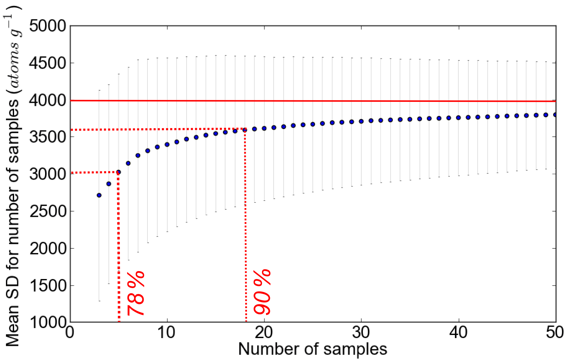
Figure 12 Number of ¹⁰Be samples required to capture the natural concentration variability of the Ganga River. Approximately 18 samples are required to be within 10 % of the true standard deviation (or variability) of the system. Blue dots represent the mean standard deviation of 100 populations of concentrations for a given sample group size (between 3 and 50). Error bars represent the standard deviation of the mean standard deviation of those 100 populations per sample group size. The solid horizontal red line represents the mean standard deviation value that the sample group sizes converge towards (4000 atoms g⁻¹). The two dashed red lines represent the number of samples required to be within 10 % of the true standard deviation (labelled 90 %) and the standard deviation expected from a set of five samples (labelled 78 %).

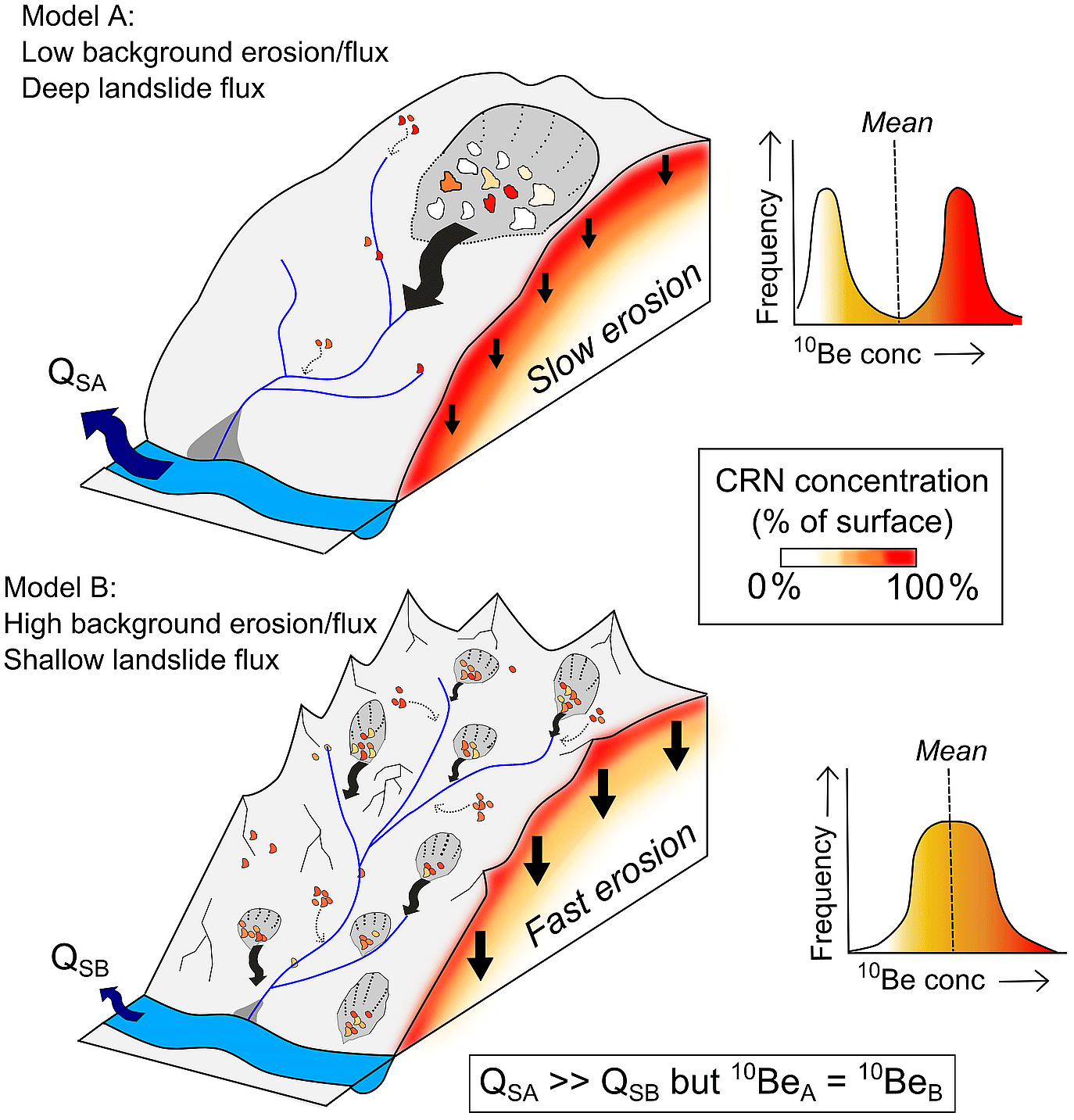
Figure 13 Schematic of how comparable mean CRN concentrations in river sand can be derived under two different end-member erosion scenarios with different volumetric sediment fluxes. In these instances, slow background erosion rates and deep landsliding (Model A) result in comparable CRN concentrations to landscapes dominated by faster background erosion rates and shallow landsliding (Model B). If Model A is set with a background erosion rate of 0.4 mm yr⁻¹ and 5 m deep landsliding over 0.5 % of the catchment, and Model B with 2 mm yr⁻¹ background erosion rates and 1 m deep landsliding (over the same area), comparable CRN concentrations (see black dots marked in Fig. 8a) and CRN-derived sediment fluxes are generated, but volumetric sediment fluxes are over 3 times larger in Model A. This is due to the relative enrichment of ¹⁰Be in the upper 2 m of the landscape with low background erosion rates, which when combined with low CRN concentration material from depth, results in two distinct CRN concentration populations. Where erosion is generally more homogeneous (Model B) and CRN concentrations are distributed more uniformly, comparable mean CRN concentrations are derived between the two models. Both scenarios assume complete mixing of the event sediment, hence why these are considered end-member or extreme scenarios.

Our results also suggest that, for ¹⁰Be concentrations within a natural degree of system variability, the volumetric sediment flux could theoretically differ from that calculated directly from ¹⁰Be concentrations (Fig. 8d and Table 3). Similar outlet ¹⁰Be concentrations could be derived from landscapes dominated by different erosional processes within large catchments. For example, our analysis suggests that a “fast-eroding” landscape experiencing a background erosion rate of 2.0 mm yr⁻¹ and 1 m deep landslides over 0.5 % of the catchment (e.g. a landscape dominated by shallow landsliding or debris flows) could produce comparable outlet ¹⁰Be concentrations to a “slow-eroding” landscape experiencing 0.4 mm yr⁻¹ background erosion and 5.0 m deep landslides over the same area (e.g. a landscape experiencing deep earthflows) (Fig. 13). The CRN-derived sediment fluxes between these two landscapes may be comparable, but the volumetric flux from the landscape with lower background erosion (and deeper landsliding) is considerably larger than from the landscape with higher background erosion (and shallower landsliding). Halving the area affected by landsliding in only the lower background erosion scenario (with deeper landsliding) still yields comparable CRN-derived fluxes (within 15 % of each other, rather than 6 %), but the volumetric flux is double that generated under higher background erosion rates (with shallower landsliding over a larger area). These types of “slow-eroding” landscapes which experience episodes of mass wasting are exemplified by arid parts of the northwest Himalaya, which generally only experience high-intensity rainstorms during abnormal monsoon years where the ISM can penetrate north of the orographic barrier formed by the Higher Himalaya (Bookhagen et al., 2005) (Fig. 2). Similarly, slow-moving earthflows in parts of the Eel River catchment in California which is characterised by long and low-gradient hillslopes mobilise huge quantities of sediment which contribute to the majority of the suspended sediment flux from the catchment (Mackey and Roering, 2011). The two end-member models presented in Fig. 13 suggest that, under different geomorphic process domains, comparable mean ¹⁰Be concentrations could theoretically be produced through different ¹⁰Be concentration populations.

CRN-derived sediment fluxes are based on an average landscape lowering rate and thus fail to incorporate the effects of spatially limited deeper inputs of sediment which are characterised by much lower ¹⁰Be concentrations. Lower rates of background erosion mean that sediment eroded off the surface is enriched in ¹⁰Be (as sediment residence times in the upper 1–2 m of the Earth's surface are longer as a function of lower background erosion rates). This effectively averages out the influence of lower concentration input from deeper inputs and results in near identical ¹⁰Be concentrations at the mountain front to a system undergoing only a slightly faster (or more uniform) rate of background erosion. Thus, considerably different volumetric fluxes can be obtained for the same ¹⁰Be concentration. However, our analysis has also shown that spatially variable erosion rates and event buffering can alter this relationship, such that CRN-derived and volumetric sediment fluxes can be comparable. Furthermore, under particular conditions, it is possible to generate systems where the effects of large sediment-generating events are lost within the natural variability of the system. This may explain the absence of a ¹⁰Be concentration signature of Holocene climate change.

6 Conclusions

We present ¹⁰Be analysis from a variety of modern and Holocene sedimentary deposits in a large trans-Himalayan catchment spanning more than 7000 m in relief, where sediment production is heavily influenced by stochastic inputs. We find a natural degree of variability in ¹⁰Be concentrations documented in the modern channel and Holocene flood deposits preserved near the catchment outlet. These concentrations appear insensitive to regional intensification of the ISM, thought to have occurred ∼11–7 ka. We suggest that the observed variability is driven by (1) the nature of the stochastic inputs of sediment (e.g. the type of hillslope process, surface ¹⁰Be production rates, degree of mixing) and (2) the evacuation timescales of these sediment deposits. Sediment deposits generated by processes such as earthquake-induced landsliding, GLOFs or storm events are typically large in volume and low in ¹⁰Be concentration, but the time taken to mobilise this sediment out of the catchment limits its impact on catchment-averaged concentrations. We suggest that, in landscapes characterised by high topographic relief, spatially variable climate and multiple geomorphic process domains, the use of ¹⁰Be concentrations to generate sediment flux estimates may not be truly representative, as comparable mean catchment ¹⁰Be concentrations can be derived through dramatically different erosional processes. For a given ¹⁰Be concentration, volumetric sediment flux estimates may vary and, under certain conditions, ¹⁰Be concentrations may under-estimate actual erosion rates and hence sediment flux. Future sampling strategies in large Himalayan catchments should seek to incorporate multiple samples in both monsoon and non-monsoon conditions to better characterise temporal variability in ¹⁰Be concentrations.

Appendix A

The details and context of cosmogenic radionuclide samples used in this study are presented in Figs. A1–A16. Locations can also be found in more detail in Fig. 3.

Figure A1 BGM – sieved from upper layer of modern gravel bar; 82 mm long penknife in base of pit.

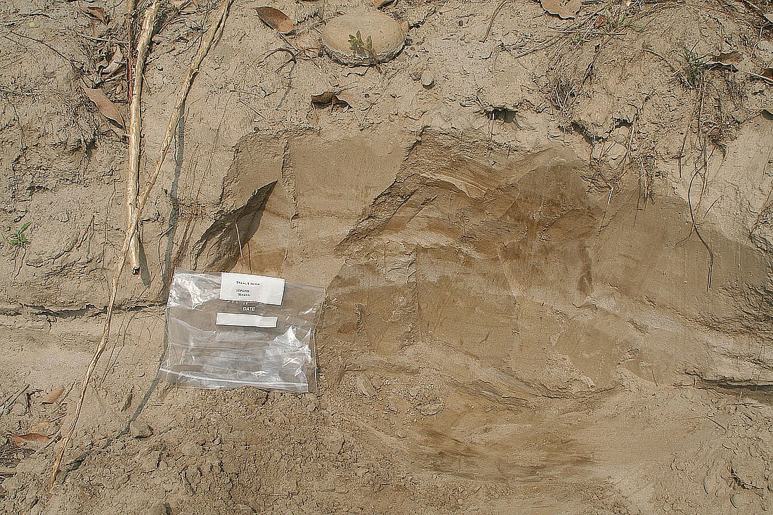
Figure A2 BG1.8 – fine-grained sand deposit (∼7 m in thickness) corresponding to sequence of palaeo-flood deposits from last ∼600 years. Sample was taken 1.8 m from base of exposure which has been OSL dated at 225±72 years (Wasson et al., 2013).

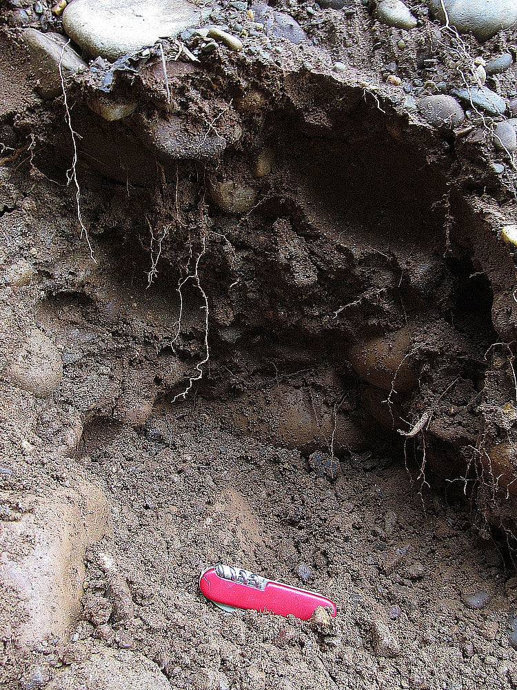
Figure A3 CDT3 – sample from base of ∼3.2 m thick fill of poorly sorted fluvial pebble and cobble conglomerate, suggesting it was deposited during a single event (approximately 26 m above the modern channel). OSL dated at 9760±1040 years (Ray and Srivastava, 2010); 90 mm long penknife for scale.

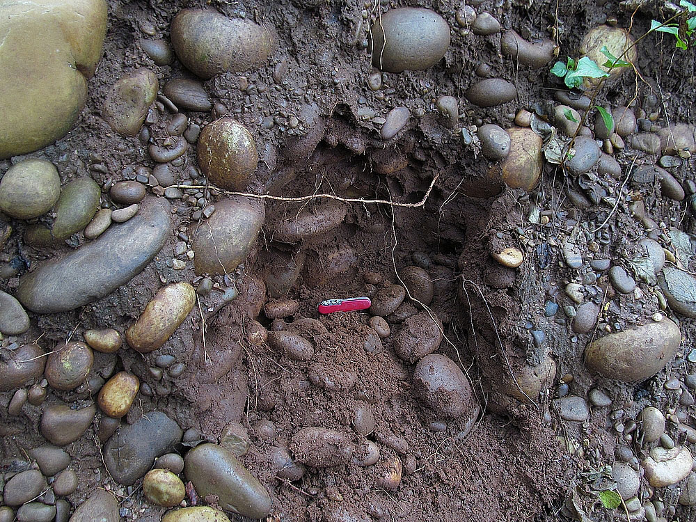
Figure A4 CDT4 – sample from poorly sorted fluvial pebble and cobble conglomerate terrace fill deposited during a single event. Sample is ∼3 m below terrace surface and ∼80 m above modern channel. OSL dated at 11 080±1960 years (Ray and Srivastava, 2010); 90 mm long penknife for scale.

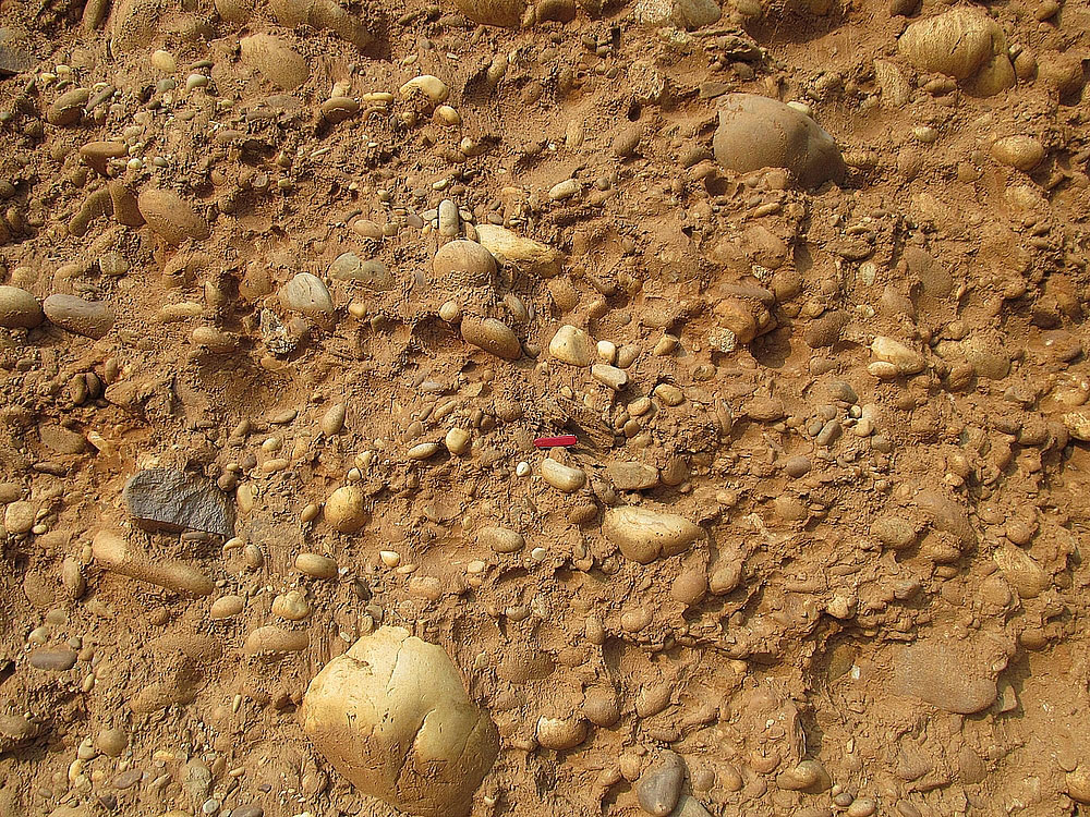
Figure A5 DVDF – terrace deposit ∼95 m above modern channel. Sample was taken from the base of 4 m thick fluvial conglomerate layer, capped by more angular phyllite/schist deposit (erosional contact) suggesting input of locally derived landslide/debris flow material. Unit OSL dated at 10 000±2000 years (Ray and Srivastava, 2010); 90 mm long penknife for scale.

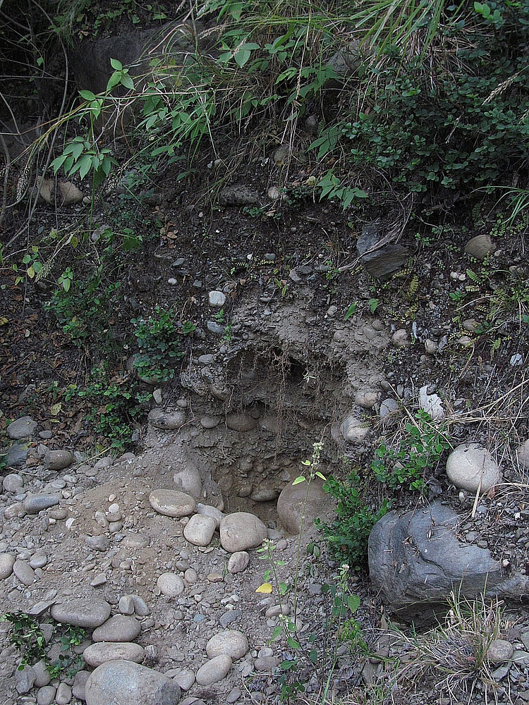
Figure A6 DVMT2 – terrace deposit ∼77 m above modern channel. Poorly sorted and weakly consolidated fluvial pebble and cobble conglomerate. Sample was taken from base of 6.5 m unit. Unit OSL dated at 10 000±2000 years (Ray and Srivastava, 2010).

Figure A7 DVTT2 – terrace deposit ∼112 m above modern channel. Fluvially derived coarse cobble and sand (poorly sorted) conglomerate interbedded within locally derived (Lesser Himalayan) phyllite deposits; 90 mm long penknife for scale.

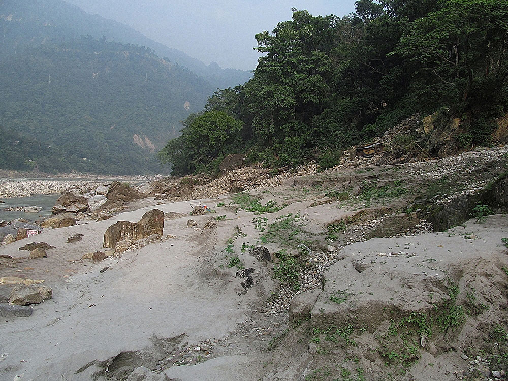
Figure A8 RFLO – sand flood deposit associated with 2013 Alaknanda flooding; ∼7 m above water level in October 2014.

Figure A9 RAEM – sieved from upper layer of modern gravel bar.

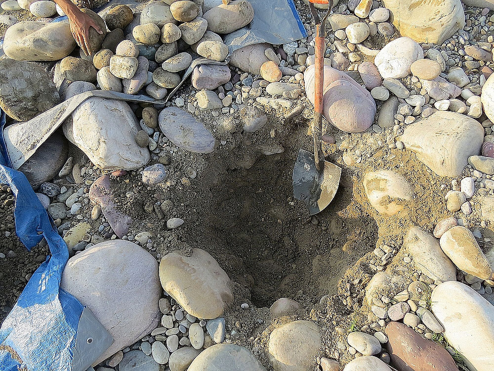
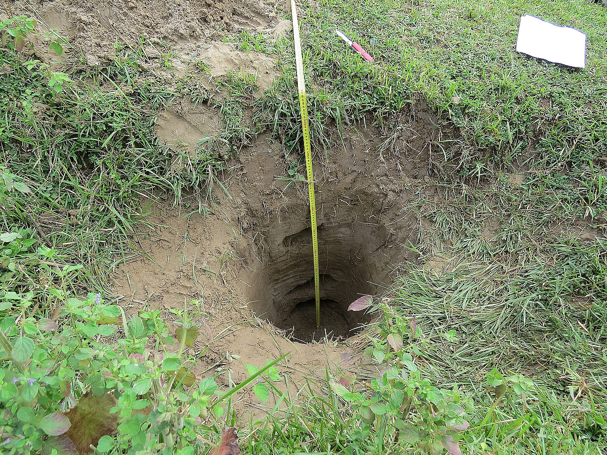
Figure A10 RAE1/RAE2 – ∼0.8 m thick sand and silt deposit above cobble bed, capped by ∼30–50 cm of soil. Samples were taken from the lower-most and middle units identified in P1 in Wasson et al. (2013) which are dated at 2.6±0.6 ka and 1.0±0.2 ka, respectively.

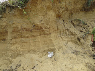
Figure A11 NGM – cross-bedded sand succession ∼17 m above modern channel. Sample was taken from base of 1.5 m thick cross-bedded sand unit. Top of unit (S2) OSL dated at 7200±2000 years by Sinha et al. (2010).

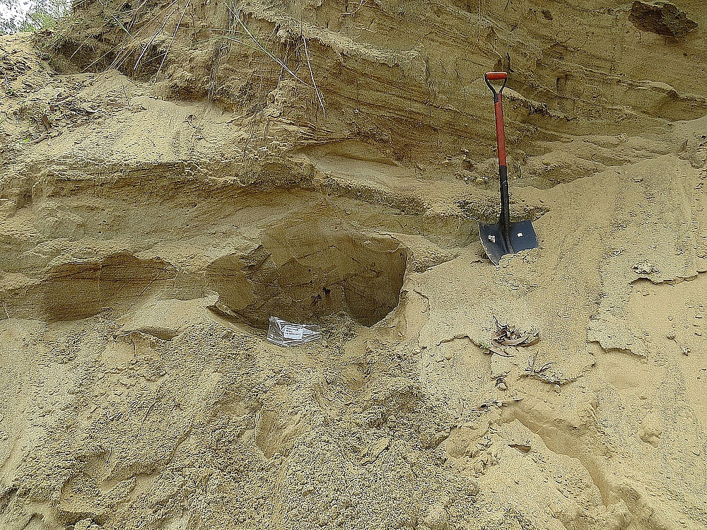
Figure A12 NGL – cross-bedded medium-coarse sand unit ∼10 m above modern channel. Base of unit (S1) OSL dated at 14 000±3000 years by Sinha et al. (2010).

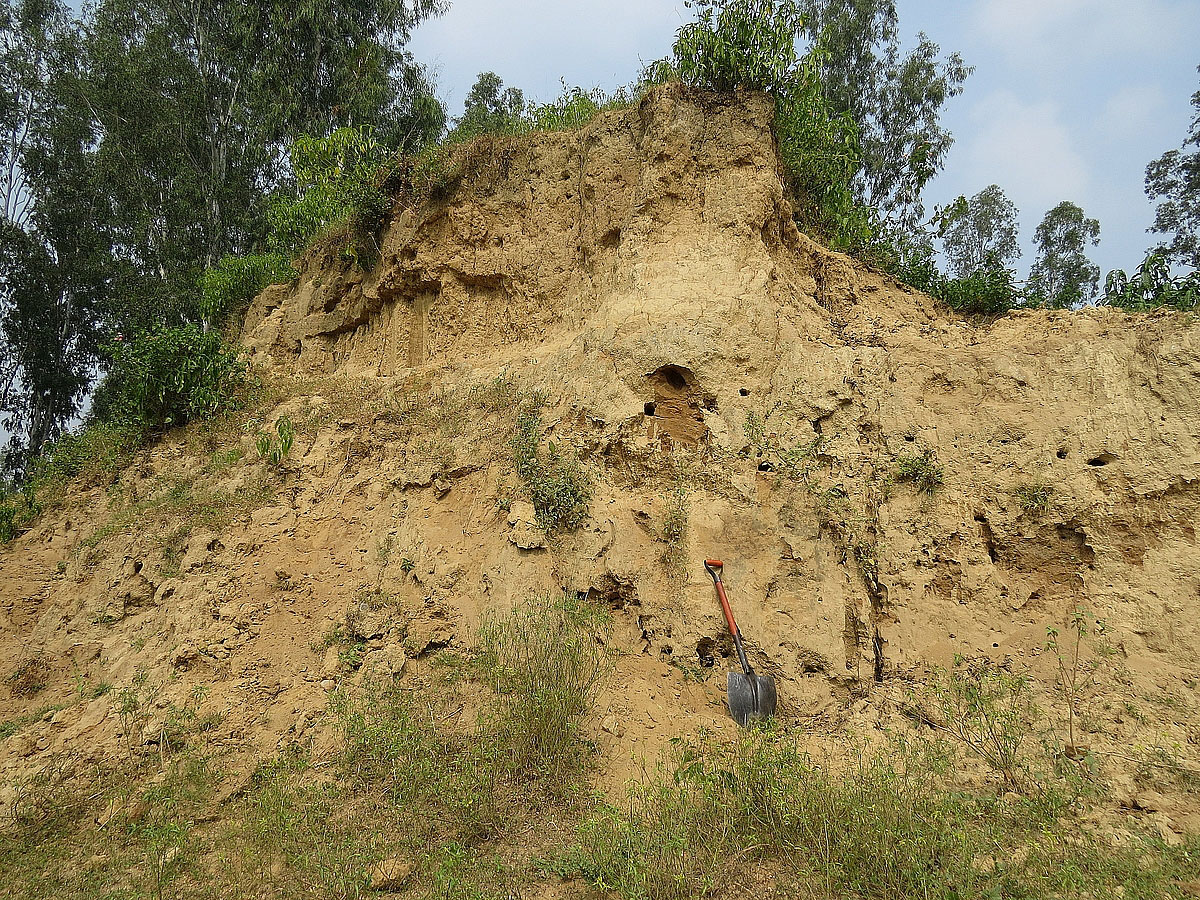
Figure A13 NGT – 4 m high exposure of low angle cross-bedded sands, topped with finer silt and mud deposits, corresponding to OSL sample from this part of unit dated at 7200±2000 years by Sinha et al. (2010).

Figure A14 LH – cross-bedded sand exposure (4 m high). Sample was taken 2.2 m from top of exposure, corresponding to OSL sample from unit dated at 23 500±1500 years by Verma (2016).

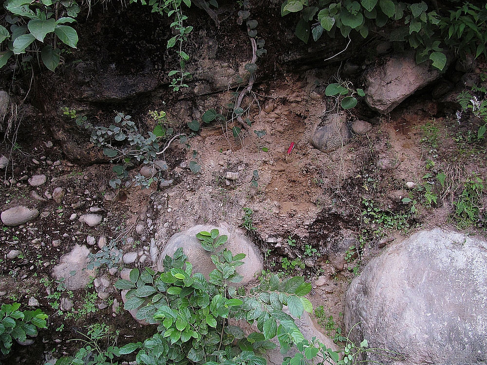
Figure A15 RLB – ∼42 m above modern channel on roadside cut. Poorly sorted, structureless fluvial conglomerate. Large, rounded boulders, cobbles and sands (Ray and Srivastava, 2010); 90 mm long penknife for scale.

Figure A16 DV2013 – laminated sand deposit ∼5 to 10 m thick formed in single event following the 2013 Alaknanda flooding.

Table A1 Additional CRN sample details.