Effect of changing vegetation and precipitation on denudation – Part 2: Predicted landscape response to transient climate and vegetation cover over millennial to million-year timescales

We present a numerical modeling investigation into the interactions between transient climate and vegetation cover with hillslope and detachment limited fluvial processes. Model simulations were designed to investigate topographic patterns and behavior resulting from changing climate and the associated changes in surface vegetation cover. The Landlab surface process model was modified to evaluate the effects of temporal variations in vegetation cover on hillslope diffusion and fluvial erosion. A suite of simulations were conducted to represent present-day climatic conditions and satellite derived vegetation cover at four different research areas in the Chilean Coastal Cordillera. These simulations included steady-state simulations as well as transient simulations with forcings in either climate or vegetation cover over millennial to million-year timescales. Two different transient variations in climate and vegetation cover including a step change in climate or vegetation were used, as well as 100 kyr oscillations over 5 Myr. We conducted eight different step-change simulations for positive and negative perturbations in either vegetation cover or climate and six simulations with oscillating transient forcings for either vegetation cover, climate, or oscillations in both vegetation cover and climate. Results indicate that the coupled influence of surface vegetation cover and mean annual precipitation shifts basin landforms towards a new steady state, with the magnitude of the change being highly sensitive to the initial vegetation and climate conditions of the basin. Dry, non-vegetated basins show higher magnitudes of adjustment than basins that are situated in wetter conditions with higher vegetation cover. For coupled conditions when surface vegetation cover and mean annual precipitation change simultaneously, the landscape response tends to be weaker. When vegetation cover and mean annual precipitation change independently from one another, higher magnitude shifts in topographic metrics are predicted. Changes in vegetation cover show a higher impact on topography for low initial surface cover values; however, for areas with high initial surface cover, the effect of changes in precipitation dominate the formation of landscapes. This study demonstrates the sensitivity of catchment characteristics to different transient forcings in vegetation cover and mean annual precipitation, with initial vegetation and climate conditions playing a crucial role.

1 Introduction

Plants cover most of the Earth's surface and interact chemically and physically with the atmosphere, lithosphere, and hydrosphere. The abundance and distribution of plants throughout Earth's history is a function, amongst other things, of changing climate conditions that can impact the temporal distribution of plant functional types and the vegetation cover present in an area (Hughes, 2000; Muhs et al., 2001; Walther et al., 2002). The physical feedbacks of vegetation on the Earth's near surface mainly manifest themselves through the influence of plants on weathering, erosion, transport, and the deposition of sediments (Marston, 2010; Amundson et al., 2015). Although the effects of biota on surface processes has been recognized for over a 100 years (e.g., Gilbert, 1877; Langbein and Schumm, 1958), early studies mainly focused on qualitative descriptions of the underlying processes. With the rise of new techniques to quantify mass transport from the plot-scale to the catchment-scale, and the emergence of improved computing techniques and landscape evolution models, research has shifted more towards building a quantitative understanding of how biota influence both hillslope and fluvial processes (Stephan and Gutknecht, 2002; Roering et al., 2002; Marston, 2010; Curran and Hession, 2013). These previous studies motivate the companion papers presented here. In part 1 (Werner et al., 2018) a dynamic vegetation model is used to evaluate the magnitude of past (last glacial maximum to present) vegetation change along the climate and ecological gradient in the Coastal Cordillera of Chile. Part 2 (this study) presents a sensitivity analysis of how transient climate and vegetation impact catchment denudation. This component is evaluated through the implementation of transient vegetation effects for hillslopes and detachment limited rivers in a landscape evolution model.

Previous research in agricultural engineering has focused on plot-scale models to predict total soil loss in response to land use change (Zhou et al., 2006; Feng et al., 2010) or general changes in plant surface cover (Gyssels et al., 2005); however, previous studies do not draw conclusions about large-scale geomorphic feedbacks active over longer (millennial) timescales and larger spatial scales. Nevertheless, a better understanding of how vegetation influences the large-scale topographic features (e.g., relief, hillslope angles, and catchment denudation) is crucial to understanding the evolution of modern landscapes. At the catchment scale, observational studies have found a correlation between higher values of mean vegetation cover and basin wide denudation rates or topographic metrics (Jeffery et al., 2014; Sangireddy et al., 2016; Acosta et al., 2015). Parallel to the previous observational studies, numerical modeling experiments of the interactions between landscape erosion and surface vegetation cover have also made progress. For example, Collins et al. (2004) was one of the first studies that attempted to couple vegetation dynamics with a landscape evolution model; they found that the introduction of plants to their model resulted in steeper equilibrium landscapes with a higher variability in the magnitude of erosional events. Following this, subsequent modeling studies built upon the previous findings with more sophisticated formulations of vegetation–erosion interactions (Istanbulluoglu and Bras, 2005), including the influence of root strength on hillslopes (Vergani et al., 2017). These studies found that not only is there a positive relationship between vegetation cover and mean catchment slope and elevation, but an inverse relationship also exists between vegetation cover and drainage density due to plants' abilities to hinder fluvial erosion and channel initiation.

The advances of the previous studies are mainly limited by their consideration of static vegetation cover or very simple formulations of dynamic vegetation cover. The exceptions to this are Istanbulluoglu and Bras (2005) who also considered the lag time for vegetation regrowth on hillslopes after a mass wasting event and Yetemen et al. (2015) who considered more complex hydrology in their models, but on a smaller spatial scale. However, numerous studies (Ledru et al., 1997; Allen and Breshears, 1998; Bachelet et al., 2003) document that vegetation cover changes in tandem with climate change over a range of timescales (decadal to million year). Missing from previous landscape evolution studies, is consideration of not only how transient vegetation cover influences catchment denudation, but also how coeval changes in precipitation influence catchment-wide mean denudation. While the effects of climate change over geologic timescales on denudation rates and sediment transport dynamics have been investigated by others (e.g., Schaller et al., 2002; Dosetto et al., 2010; McPhillips et al., 2013), the combined effects of vegetation and climate change on catchment denudation have not. Thus, over longer (geologic) timescales, we are left with a complicated situation of both vegetation and climate changes, and the individual contributions of these changes to catchment-scale denudation are difficult to disentangle.

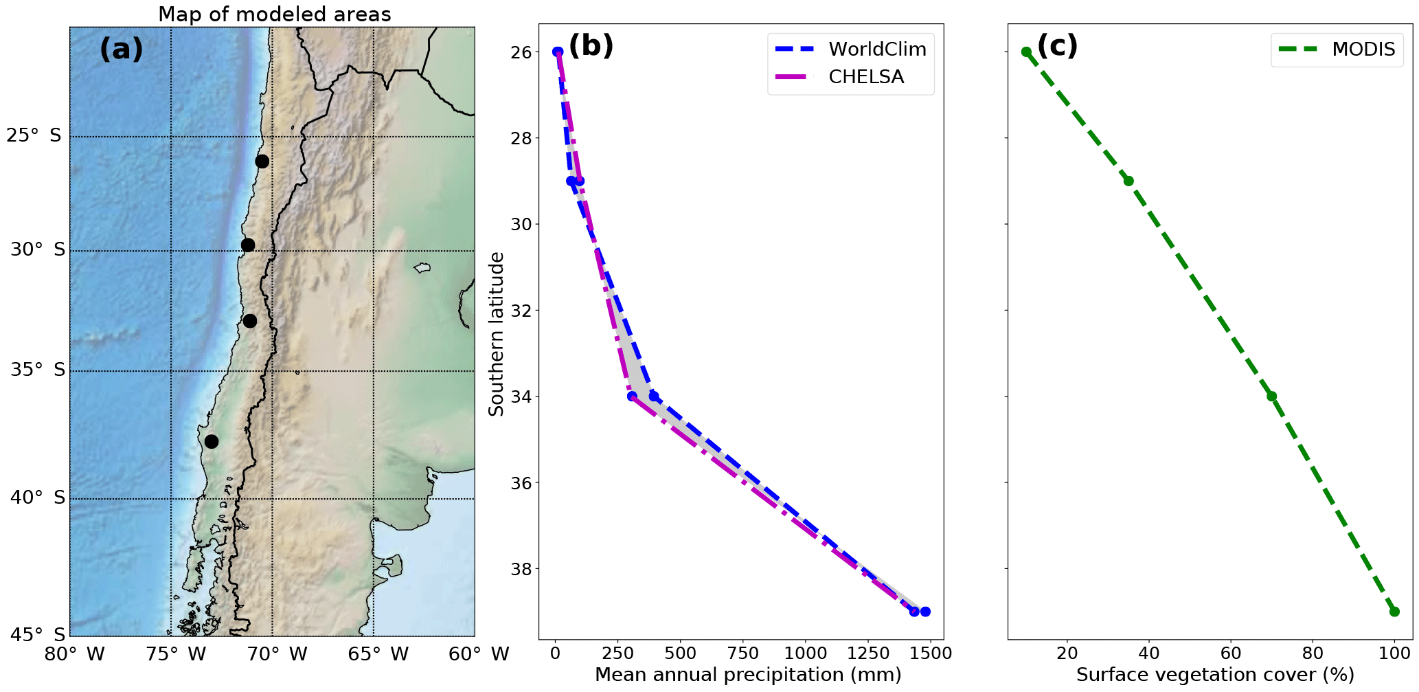
Figure 1 Overview of the geographic location, precipitation, and vegetation cover of the Chilean Coastal Cordillera study areas used for the model setup. (a) Digital topography of the areas considered in this study, which correspond to the EarthShape (https://www.earthshape.net) focus areas where ongoing related research is located. (b) Observed present-day mean annual precipitation from the WorldClim and CHELSA datasets used as model input. (b) Present-day maximum surface vegetation cover from MODIS data.

In this study, we build upon previous research by investigating both the temporal and spatial sensitivities of landscapes to the coupled vegetation–climate system. By focusing on simplified transient forcings such as a step change, or 100 kyr oscillations in climate and vegetation cover we present a sensitivity analysis of the landscape response to each of these changes, including a better understanding of the direction, magnitude, and rates of landscape change. Our model setup is motivated by four study areas along the climate and vegetation gradient in Chile (Fig. 1a), and illuminates the transient catchment response to biotic vs. climate changes. These study areas are part of the recently initiated German priority research program EarthShape: Earth surface shaping by biota (https://www.earthshape.net, last access: 7 August 2018). This region is used to provide a basis for our model setup regarding covariation in precipitation and vegetation present in a natural setting. While we present results representative of the Chilean Coastal Cordillera, it is beyond the scope of this study to provide a detailed calibration for this area. Hence, our main objective is identifying the sensitivity and emergent behavior of catchment denudation to changing precipitation and vegetation cover over millennial timescales. This study also builds upon results from the companion paper (Werner et al., 2018) by imposing temporal variations in vegetation cover identified in that study.

2 Background for the model setup

The model setup and the range of initial conditions chosen for the models were based on four study areas located in the Chilean Coastal Cordillera (26 to 38^∘ S). The focus areas shown in Fig. 1a were chosen due to their similar granitic lithology and geologic and tectonic history (Andriessen and Reutter, 1994; McInnes et al., 1999; Juez-Larré et al., 2010; Maksaev and Zentilli, 1999; Avdievitch et al., 2018), in addition to the large gradient in climate and vegetation cover over the region (Fig. 1b, c). These study areas include (from north to south): Pan de Azúcar National Park, Santa Gracia Natural Reserve, La Campana National Park, and Nahuelbuta National Park. Although this study does not explicitly present landscape evolution model results “calibrated” to these specific areas, we have chosen the model input (e.g., precipitation, initial vegetation cover, rate of tectonic rock uplift) to represent these areas. This has been done in order to provide simulation results that represent the nonlinear relationship between precipitation and vegetation cover (e.g., Fig. 1b, c) over a large climate gradient.

Topographic metrics such as mean basin slope, total basin relief, mean basin channel steepness, mean surface vegetation cover, and mean annual precipitation were extracted for the main catchments and a subset of adjacent catchments (Figs. 1, 2). Topographic metrics were extracted from a 30 m resolution digital elevation model from the NASA shuttle radar topography mission (SRTM), and vegetation related datasets from the Moderate Resolution Imaging Spectroradiometer (MODIS) satellite data (https://landcover.usgs.gov/green_veg.php, last access: 7 August 2018) (Broxton et al., 2014).

Landscape evolution modeling approach and the applicability of these results

Landscape evolution model studies can be assigned to different general approaches, which were conceptually defined by Dietrich et al. (2013). The different approaches presented in the Dietrich et al. (2013) study mostly differ in the complexity of the input parameters and in the resulting claim for reproducing realistic complexity in modeled landscapes. For this study we have chosen the approach of essential realism, which acknowledges a system-inherent indeterminacy in the evolving topography but focuses on predicting the first-order trends within a system and the differences between landscapes, based on different external conditions, incorporated in the model (Howard, 1997).

While we do not claim to reproduce the topographic metrics of the four different focus areas in Chile on a realistic level, our approach determines the general first-order effects of millennial timescale changes in precipitation and vegetation cover that can impact topography. Superimposed on the effects documented in this study would be the effects of seasonal changes in precipitation and vegetation cover, subcatchment variations in vegetation cover, transport limited fluvial and vegetation interactions, and stochastic variations in precipitation in different climate zones. This being said, more detailed aspects of the effects of precipitation–vegetation interactions on erosion could be independent studies of their own and can not be covered in a single study. Thus, the modeling approach and results of this study should be considered as documenting the longer (millennial) timescale climate and vegetation forcings on fluvial and surface processes.

3 Methods

3.1 Model description and governing equations

For this study, we use the open-source model framework Landlab (Hobley et al., 2017). We chose a model domain with an area of 100 km² that is implemented as a rectangular grid divided into 0.01 km² spaced grid cells. For simplification in the presentation of results, we present our results for the driest, northern most area (Pan de Azucar National Park) and for La Campana National Park. La Campana National Park is situated at 32^∘ S latitude (Fig. 1) and shows the highest values in analyzed basin metrics (Fig. 2), although the general behavior and results presented here are also representative of the other two areas (not shown). The topographic evolution of the landscape is a result of tectonic uplift and surface processes, incorporating detachment limited fluvial erosion and linear diffusive transport of sediment across hillslopes (Fig. 3). These processes are linked to, and vary in their effectiveness due to, surface vegetation density. Details of the implementation of these processes in Landlab are explained in the following subsections.

Figure 2 Normalized basin metrics for study areas derived from 30 m SRTM digital topography (from the study areas shown in Fig. 1a). Colored dots represent cumulative mean values of normalized slope, relief, and channel steepness calculated for all locations using five to eight representative catchments in each area. Dotted lines represent linear interpolation between values. Note the gradual increase, then decrease in all metrics around study area at ∼32^∘ S.

Table 1 Model parameters used for the Landlab model setup.

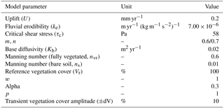
This model setup is simplified with regards to hydrological parameters such as soil moisture and groundwater and unsaturated zone flow. Furthermore, the erosion and transport of material due to mass-wasting processes such as rockfalls and landslides are not considered. We argue that these processes do not play a major role in the basins we used for model calibration, and that the processes acting continuously along hillslopes and channels have the largest impact on shaping our reference landscapes. The detachment-limited approach was chosen because the focus areas represent small, bedrock dominated headwater catchments. Additional caveats and limitations of the modeling approach used are discussed in Sect. 5.4. Main model parameters used in the model (and described below) are provided in Table 1.

3.2 Boundary and initial conditions and model free parameters

In an effort to keep simulations comparable, we minimized the differences in parameters between simulations. The exceptions to this include the surface vegetation cover and the mean annual precipitation, which were varied between simulations. One of the main controls on topography is the rock uplift rate. We kept the rock uplift rate temporally and spatially uniform across the domain at 0.2 mm yr⁻¹ (Table 1). Studies of the exhumation and rock uplift history of the Chilean Coastal Cordillera are sparse at the latitudes investigated here; however, existing and in progress studies further to the north are broadly consistent with the rock uplift rate used here (Juez-Larré et al., 2010; Avdievitch et al., 2018).

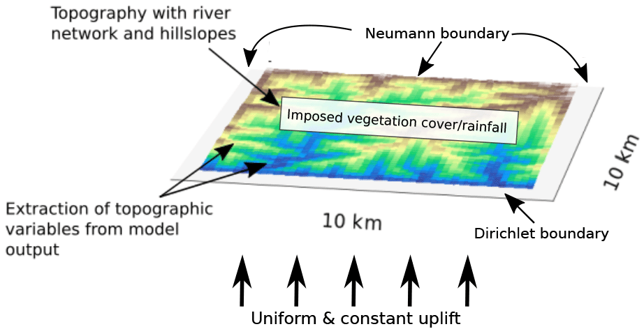
Figure 3 An example of the model setup used in the simulations in this study, showing model predicted topography with a set drainage network, draining to the south. Boundary conditions and parameterizations used in the models are labeled. Blue represents low elevations and brown represents higher elevations. Additional details of parameters used are specified in Table 1.

The EarthShape focus sites are situated in similar granitic lithologies (Oeser et al., 2018), which allows for the assumption that the same critical shear stress, baseline diffusivity, and fluvial erodibility can be used.

Vegetation cover was chosen to be spatially uniform across model domains. While vegetation can change in high-relief catchments due to precipitation and temperature changes with elevation, this simplifying assumption was made based on the low to moderate relief (500–1500 m, mean ∼750 m) of the Coastal Cordillera areas investigated, in addition to the minimal field and MODIS observed changes in type and cover with elevation. The exception to this was the La Campana study area (∼1500 m relief), which had an observed change in vegetation type and cover in the upper 500 m of the catchment. Furthermore, dynamic vegetation modeling results presented in the companion paper “part 1” (Fig. 5b in Werner et al., 2018) indicate that although elevation gradients in plant functional types have occurred in the region since the last glacial maximum, the elevation range of the catchments in the Coastal Cordillera (<1500 m) exhibits only minor changes with elevation. Vegetation cover near trunk streams within catchments is observed (via field observations) to increase, most likely due to local-scale hydrology and more abundant water in these areas. However, these regions are often restricted to with tens of meters of the trunk stream, well below the 100 m grid resolution of the model; therefore, they are difficult to accurately resolve within the simulations presented.

The initial topography used in our simulations was a random white-noise topography with <1 m relief. To avoid unwanted transients related to the formation of this initial topography we conducted simulations to produce an equilibrium topography for each set of the different climate and vegetation scenarios (see below). These equilibrium topographies were produced by running the model for 15 Myr until a topographic steady state was reached. The equilibrium topography after 15 Myr was used as the input topography for subsequent experiments that imposed transient forcings in climate, vegetation, or both (Fig. 4). The model simulation time shown in subsequent plots is the time since the completion of this initial 15 Myr steady-state topography development. In the results section, we present these results starting with differences in the initial steady-state topographies (prior to imposing transient forcings) and then add different levels of complexity by imposing either (1) a single transient step change for the vegetation cover (Fig. 4b), (2) a step change in the mean annual precipitation (Fig. 4d), (3) 100 kyr oscillations in the vegetation cover (Fig. 4a), (4) 100 kyr oscillations in the mean annual precipitation (Fig. 4c), or (5) 100 kyr oscillation in both the vegetation cover and mean annual precipitation (both Fig. 4a and c). This approach was used to produce a stepwise increase in model complexity for evaluating the individual, and then the combined, effects of fluvial and hillslope processes to different forcings.

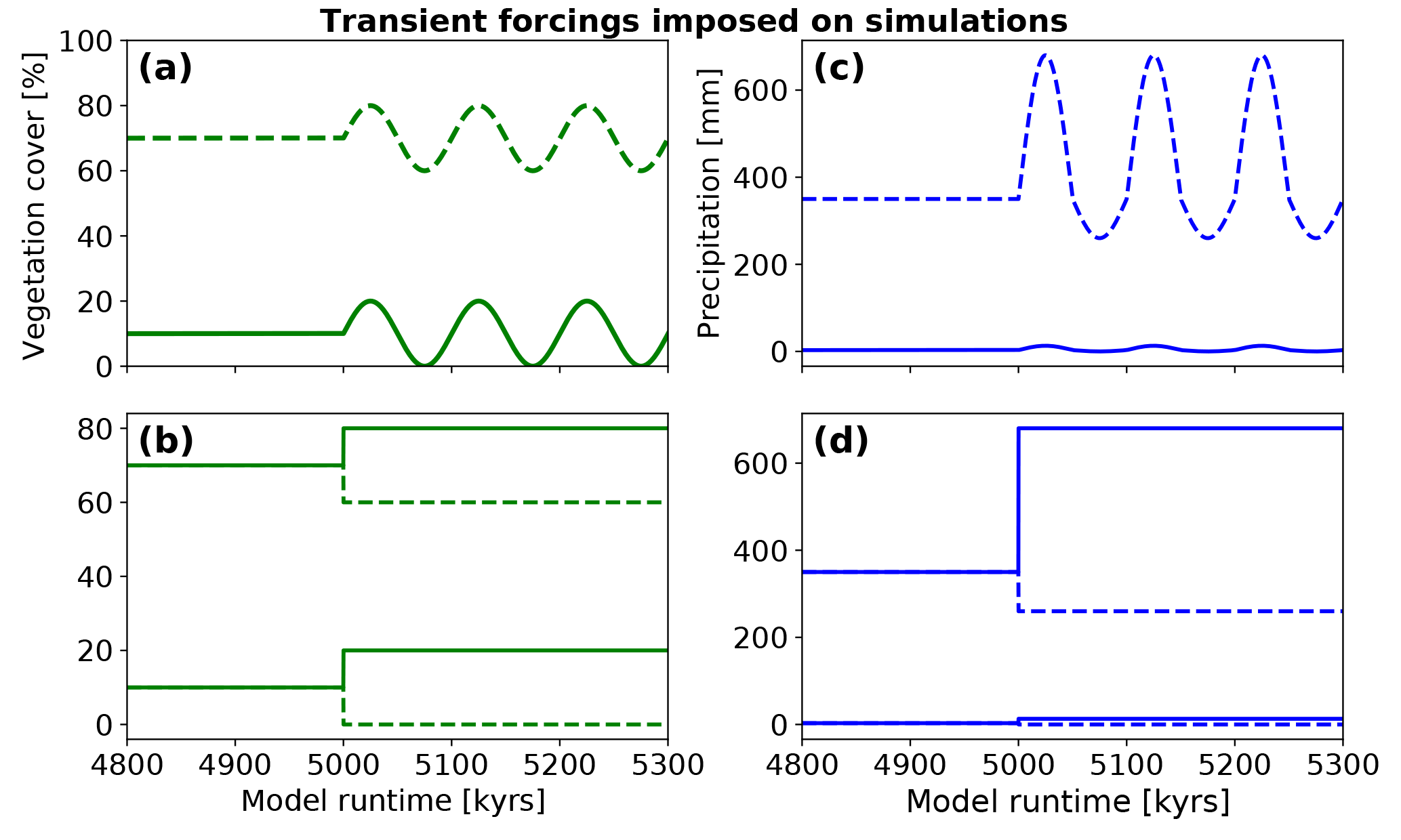
Figure 4 Transient forcings in vegetation and precipitation considered in model experiments. Simulations were run for 15 Myr prior to the runtime shown in the figure. All transients imposed started at a runtime of 5 Myr. (a) Variations in vegetation cover imposed in the oscillating experiment conditions for an initial vegetation cover of 10 and 70 %. Oscillations have a 10 % amplitude and a 100 kyr periodicity. (b) 10 % positive and negative step changes in vegetation cover imposed on simulations with 10 % and 70 % initial vegetation cover. (c) Oscillating mean annual precipitation. Positive and negative amplitudes of oscillation resemble the magnitude of precipitation change extracted from the vegetation cover–rainfall relationship from satellite data (Fig. 5). (d) Positive and negative step changes in mean annual precipitation. The initial precipitation was based on values extracted from the WorldClim climate dataset for respective focus areas.

The magnitude of induced rainfall transient forcings were based upon the present-day conditions along the Coastal Cordillera study areas (Fig. 1b, c). The step change and oscillations in vegetation cover and mean annual precipitation imposed on the experiments were designed to investigate vegetation and precipitation change effects on topography over the last ∼0.9 Ma – the period during which a 100 kyr orbital forcing is dominant in Earth's climate (Broecker and van Donk, 1970; Muller and MacDonald, 1997). Given this timescale of interest, we impose a 10 % magnitude change in the step-increase or decrease, or the amplitude change in oscillations for the vegetation cover. This magnitude of vegetation cover change is supported by dynamic vegetation modeling of vegetation changes over glacial–interglacial cycles in Chile (see companion paper by Werner et al., 2018), and to some degree elsewhere in the world (Allen et al., 2010; Prentice et al., 2011; Huntley et al., 2013); however, for the sake of simplicity we use a fixed forcing of ±10 % for all simulations instead of a spatially variable forcing, which would be dependent on ecosystem behavior for each separate area. We assume that the present-day conditions of combined vegetation cover and mean annual precipitation along the north–south gradient of the Coastal Cordillera are directly linked (Fig. 1b, c); therefore, we follow an empirical approach based on the present-day mean annual precipitation, which directly links to the present-day vegetation cover in Chile (Fig. 5). We do this by associating each 10 % change in vegetation cover (dV) with a corresponding change in mean annual precipitation (dP, Fig. 5) present in the study areas considered. We impose a predefined, fixed amplitude change in surface vegetation cover as a transient forcing for simulations. For our prescribed changes in vegetation cover we then choose corresponding values of mean annual precipitation based on the relationship shown in Figs. 1 and 5. The simulations were parameterized in terms of changes in vegetation cover (instead of precipitation) for two reasons. First, the emphasis of this study is on advancing our knowledge of how vegetation changes impact surface processes. Given this, we wanted to present results based on reasonable changes in vegetation cover change. Second, results from the companion paper and this paper (Werner et al., 2018) suggest that the Chilean Coastal Cordillera has experienced ±10 % changes in vegetation cover over the last 21 kyr. We adopt this result in this study as the current best estimate for the changes in the study areas considered. Thus, the changes in precipitation and vegetation imposed in this study are empirically based on observations from the climate and ecological gradient in the Coastal Cordillera.

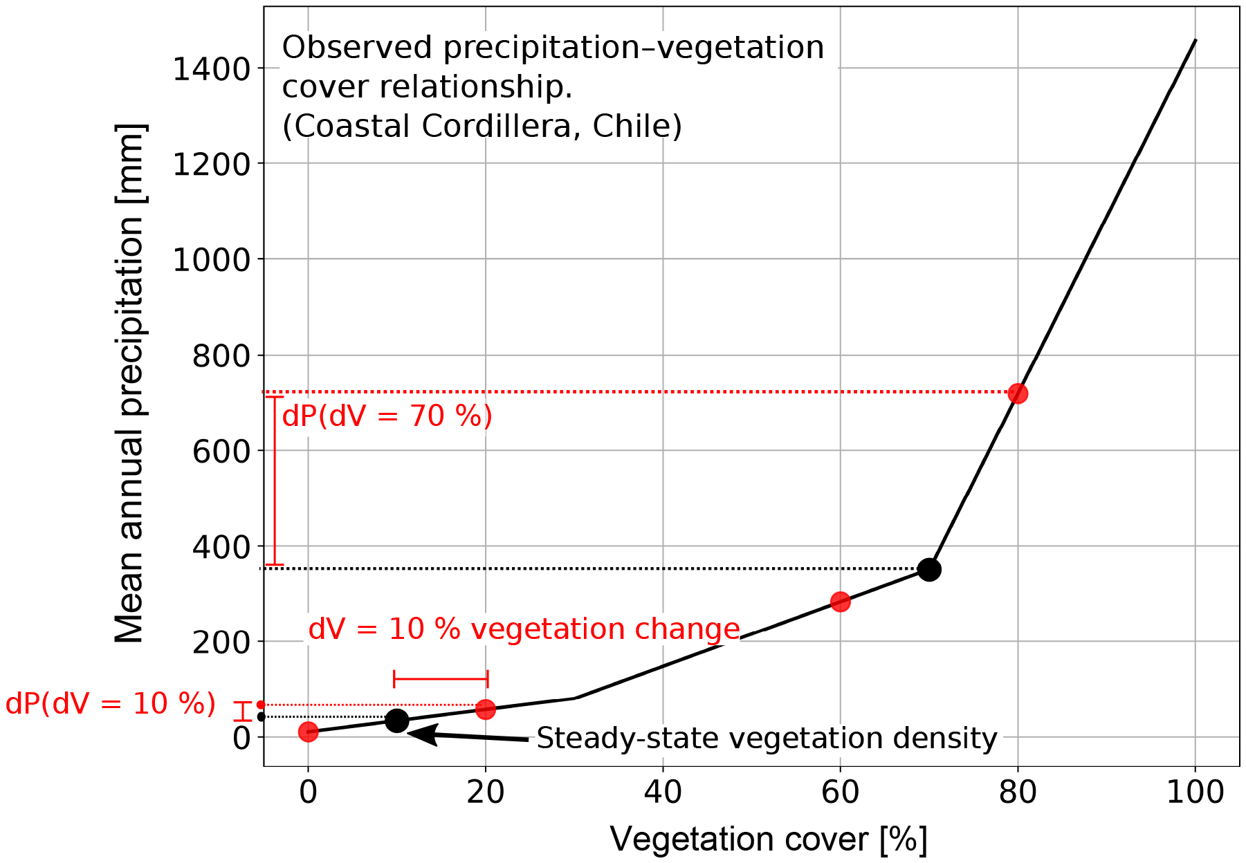
Figure 5 Graphical representation of the observed precipitation – vegetation relationship in the Chilean focus areas (shown in Fig. 1), and how precipitation amounts were selected when perturbations in vegetation cover were imposed. Black dots represent vegetation–precipitation values used in the steady-state model conditions and prior to any transients. Red dots show how vegetation cover perturbations of ±10 % in the model simulations were used to select corresponding mean annual precipitation amounts. Note that the observed relationship between observed precipitation and vegetation cover in the Chilean Coastal Cordillera is nonlinear, and is a source of the nonlinear behavior in the model forcing (e.g., Fig. 4) and results (Fig. 17) presented here.

The boundary conditions used in the model were the same for all of the simulations explained above (Fig. 3). One boundary was held at a fixed elevation and open to flow outside the domain. The other three were allowed to increase in elevation and had a zero-flux condition. This design for boundary conditions is similar to previous landscape evolution modeling studies (Istanbulluoglu and Bras, 2005), and provides a means for analyzing the effects of different vegetation cover and precipitation forcings on the individual catchment and subcatchment scale.

3.3 Vegetation cover dependent geomorphic transport laws

The governing equation used for simulating topographic change in our experiments follows the continuity of mass. Changes in elevation at different points of the model domain over time $\mathit{\delta }z(x,y,t)$ depend on the following:

$$\begin{array}{}\text{(1)}& {\displaystyle \frac{\mathit{\delta }z(x,y)}{\mathit{\delta }t}}=U-{\displaystyle \frac{\mathit{\delta }z}{\mathit{\delta }t}}{\mathrm{|}}_{\mathrm{hillslope}}-{\displaystyle \frac{\mathit{\delta }z}{\mathit{\delta }t}}{\mathrm{|}}_{\mathrm{fluvial}},\end{array}$$

where z is elevation; x, y are lateral distance; t is time; U is the rock uplift rate; $\frac{\mathit{\delta }z}{\mathit{\delta }t}{\mathrm{|}}_{\mathrm{hillslope}}$ is the change in elevation due to hillslope processes; and $\frac{\mathit{\delta }z}{\mathit{\delta }t}{\mathrm{|}}_{\mathrm{fluvial}}$ is the change in elevation due to fluvial processes (Tucker et al., 2001).

3.3.1 Vegetation cover influenced diffusive hillslope transport

The change in topography in a landscape over time caused by hillslope-dependent diffusion can be characterized as follows:

$$\begin{array}{}\text{(2)}& {\displaystyle \frac{\mathit{\delta }z}{\mathit{\delta }t}}{\mathrm{|}}_{\mathrm{hillslope}}=-\mathrm{\nabla }{q}_{\mathrm{sd}}.\end{array}$$

Landscape evolution models characterize the flux of sediment (q_sd) as either a linear or nonlinear function of surface slope (S) (Culling, 1960; Fernandez and Dietrich, 1997). In order to keep the number of free parameters for the simulation to a minimum, we used the linear description of hillslope diffusion:

$$\begin{array}{}\text{(3)}& q_{\mathrm{sd}}=K_{\mathrm{d}}S.\end{array}$$

Following the approach of Alberts et al. (1995), Dunne et al. (1995), Istanbulluoglu and Bras (2005) and Dunne et al. (2010), we assign the linear diffusion coefficient K_d as a function of the surface vegetation density V, an exponential coefficient α, and a baseline diffusivity K_b, such that

$$\begin{array}{}\text{(4)}& K_{\mathrm{d}}=K_{\mathrm{b}}{e}^{-\left(\mathit{\alpha }V\right)}.\end{array}$$

3.3.2 Vegetation cover influence on overland flow and fluvial erosion

Fluvial detachment-limited erosion of material due to water is calculated in this study by the widely used “stream power equation” (Howard and Kerby, 1983; Howard et al., 1994; Whipple and Tucker, 1999; Braun and Willet, 2013):

$$\begin{array}{}\text{(5)}& {\displaystyle \frac{\mathit{\delta }z}{\mathit{\delta }t}}{\mathrm{|}}_{\mathrm{fluvial}}=k_{\mathrm{e}}(\mathit{\tau }-{\mathit{\tau }}_{\mathrm{c}}{)}^p\mathrm{for}\mathit{\tau }>{\mathit{\tau }}_{\mathrm{c}},\end{array}$$

where k_e represents the erodibility of the bed; τ represents the bed shear stress, which acts on the surface at each node; τ_c is the critical shear stress that needs to be overcome to erode the bed material; and p is a constant.

By following the approach of Istanbulluoglu and Bras (2005) and Istanbulluoglu et al. (2004), we reformulate the standard equation of shear stress: τ_b=ρ_wgRS, where ρ_w is the density of water, g is the acceleration of gravity, R is the hydraulic radius, and S is the local slope, to a form which incorporates Manning roughness. This is undertaken in order to quantify the effect of vegetation cover on bed shear stress (Willgoose et al., 1991; Istanbulluoglu et al., 2004) and takes the following form:

$$\begin{array}{}\text{(6)}& {\mathit{\tau }}_{\mathrm{v}}={\mathit{\rho }}_{\mathrm{w}}g{\left(n_{\mathrm{s}}+n_{\mathrm{v}}\right)}^{\frac{\mathrm{6}}{\mathrm{10}}}{q}^m{S}^n{F}_t,\end{array}$$

where n_s and n_v represent Manning numbers for bare soil and vegetated ground,respectively, q is the water discharge per node that is approximated with the steady-state uniform precipitation per time step P and the surface area per node A ($q=A\times P$), S is the local slope per node, and m and n are constants. n_v for each node is calculated as a function of the local surface vegetation cover

$$\begin{array}{}\text{(7)}& n_{\mathrm{v}}=n_{\mathrm{vr}}{\left({\displaystyle \frac{V}{V_{\mathrm{r}}}}\right)}^w,\end{array}$$

with n_vr being the Manning number for a defined reference vegetation cover, V and V_r being the vegetation cover at each node and the reference vegetation cover, respectively, and w being an empirical scaling parameter.

The last variable in Eq. (6) represents the shear-stress partitioning ratio F_t (after Foster, 1982; Istanbulluoglu and Bras, 2005), which is used to scale the shear stress at each node to the vegetation cover present as follows:

$$\begin{array}{}\text{(8)}& F_t={\left({\displaystyle \frac{n_{\mathrm{s}}}{n_{\mathrm{s}}+n_{\mathrm{v}}}}\right)}^{\frac{\mathrm{3}}{\mathrm{2}}}.\end{array}$$

By combining the formulation for shear stress from Eq. (6) with the general stream power from Eq. (5), we formulate a new factor K_v that represents the bed erodibility per node as a function of surface vegetation cover. This leads to a new expression of fluvial erosion:

$$\begin{array}{}\text{(9)}& {\displaystyle }& {\displaystyle }{K}_{\mathrm{v}}=k_{\mathrm{e}}{\mathit{\rho }}_{\mathrm{w}}g{\left(n_{\mathrm{s}}+n_{\mathrm{v}}\right)}^{\frac{\mathrm{6}}{\mathrm{10}}}{F}_t\text{(10)}& {\displaystyle }& {\displaystyle \frac{\mathit{\delta }z}{\mathit{\delta }t}}{\mathrm{|}}_{\mathrm{fluvial}}=K_{\mathrm{v}}{q}^m{S}^n.\end{array}$$

An illustration of the effect of vegetation cover on K_d and K_v is presented in Fig. 6.

3.4 Model evaluation

Model performance was evaluated using the above equations and different initial vegetation covers and mean annual precipitation. Our focus in this study is on the general surface process response to different transient vegetation and climate conditions. Given this, topographic metrics of relief, mean slope, and normalized steepness index (K_sn) were computed from the model results and compared to observed values from the 30 m SRTM DEM for each of the four areas (Fig. 2). This was done to evaluate if our implementation of the governing equations in Sect. 3.4 produced topographies within reason of present-day topographies in the four Chilean areas. A more detailed model calibration is beyond the scope of this study, and not meaningful without additional observational constraints on key parameters such latitudinal variations in the rock uplift rate and erosivity. Our aim is not to reproduce the present-day topography of the Coastal Cordillera study areas, but rather to identify the sensitivity and emergent behavior of vegetation-dependent surface processes to gradients of vegetation cover and precipitation in Chile.

4 Results

Our presentation of results is structured around three groups of simulations. These groups of simulations include the following:

1. Steady-state simulations where equilibrium topographies are calculated for different magnitudes of vegetation cover and identical precipitation forcing. This includes a second set of steady-state simulations with the same magnitudes of vegetation cover as the first, but with different precipitation forcings corresponding to each vegetation cover (Fig. 5, Sect. 4.1).

2. Simulations with a transient step change in either the surface vegetation density or precipitation (Sect. 4.2) that is initiated after the landscape has reached steady state.

3. Simulations with a transient 100 kyr oscillating time series of changing vegetation or precipitation that occurs after the landscape has reached steady state (Sect. 4.3).

For each group of transient simulations, we show the topographic evolution with help of standard topographic metrics and the corresponding erosion rates after the induced change.

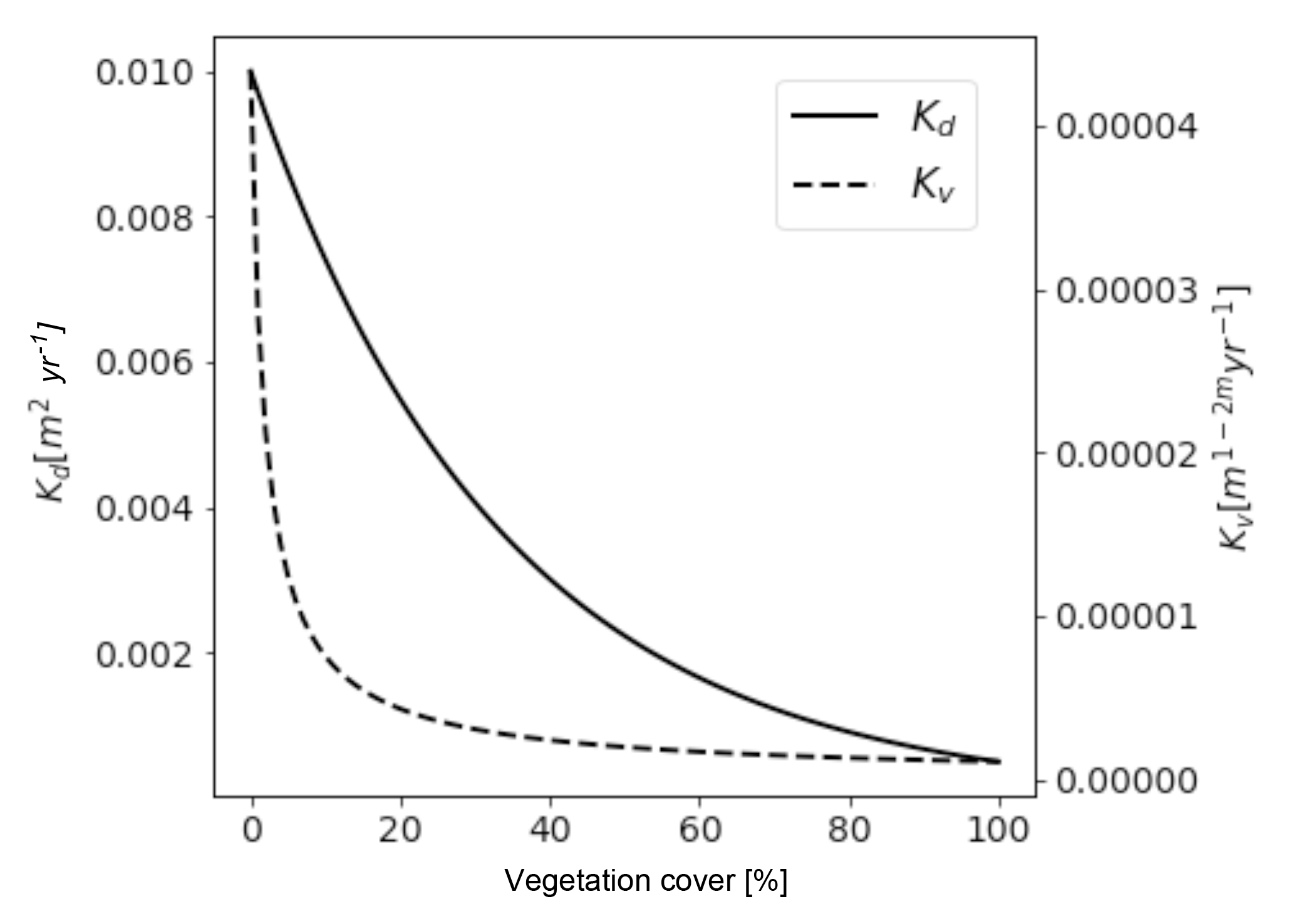
Figure 6 Predicted values of hillslope diffusivity (K_d) (solid line) and fluvial erodibility (K_v) (dashed line) as a function of vegetation surface cover. Although absolute values can not be compared due to different units, the shape of the curves representing the different parameters show different sensitivities to changes in vegetation cover. Major sources of the nonlinearities are discussed in the text. Fluvial erodibility shows the highest magnitude of change for vegetation cover values <25 %, whereas hillslope diffusivity reacts in a more linearly fashion with the highest change observed below <65 % vegetation cover.

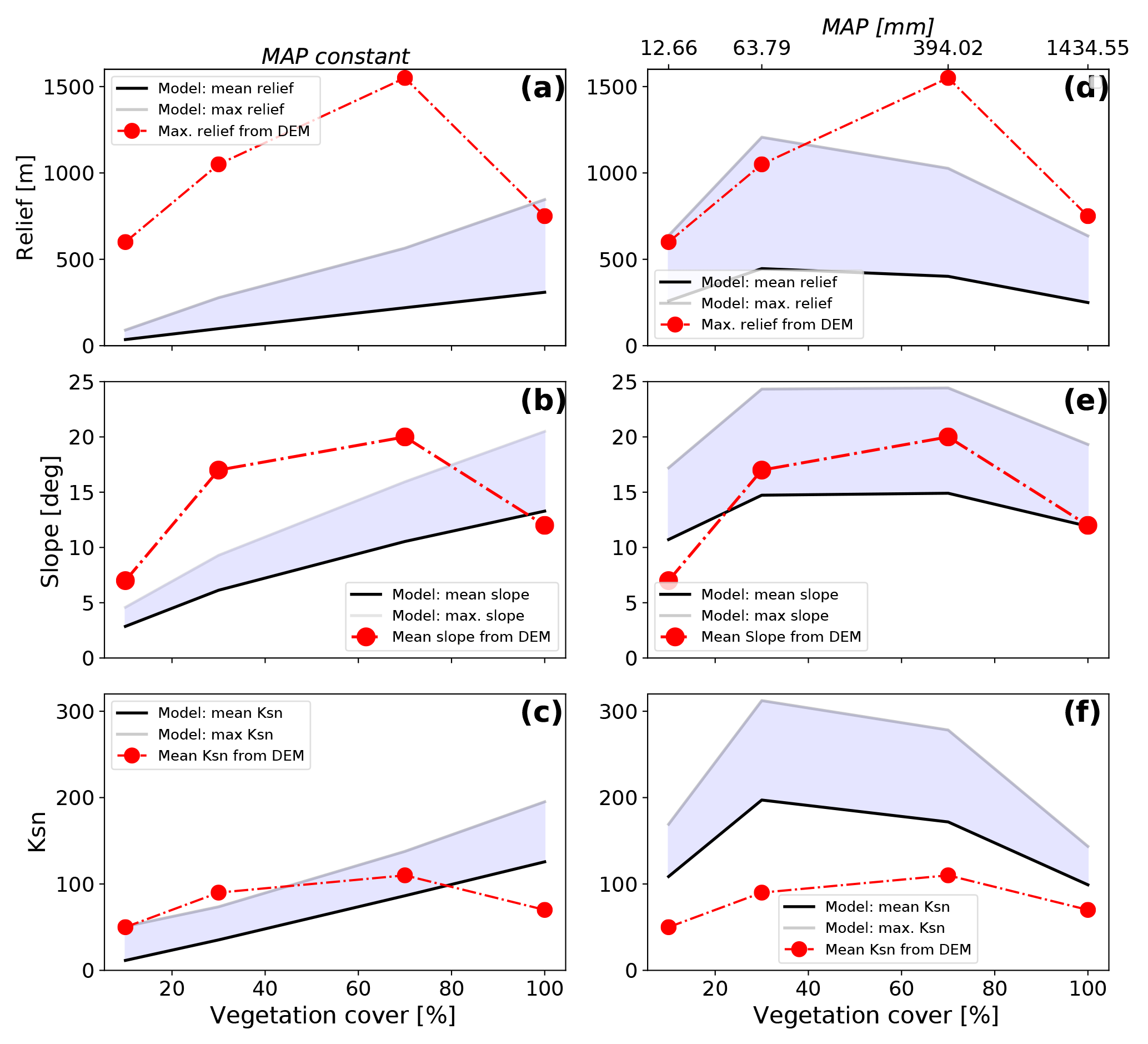
Figure 7 The steady-state model predicted (shaded regions) and observed (red dots) topographic metrics from the study areas shown in Fig. 1 for different vegetation cover amounts. Observed topographic metrics were extracted from SRTM 90 m DEM. Model predicted values are shown for the cases of constant mean annual precipitation (a, b, c) or variable precipitation (d, e, f). Variable precipitation rates and vegetation covers were selected for these simulations using the observed values from the focus areas (Fig. 5). Note that for variable precipitation and vegetation cover simulations (d, e, f) the predicted values (similar to the observations) develop a hump-shaped pattern of an increase in each parameter followed by a decrease. This suggests that changes in both precipitation and vegetation cover are needed to reproduce the general trend seen in observations. The sources of misfit between the predicted and observed values are due to the simplified (and untuned) setup of the simulations, and are discussed in the text.

4.1 Equilibrium topographic metrics

Topographic metrics from each of the four Chilean focus areas (Fig. 1a) were extracted for comparison to equilibrium topographies predicted after 15 Myr of model simulation time. This comparison was undertaken to document the model response to changing vegetation cover (with the climate held constant) and changing vegetation cover and precipitation, but also to demonstrate the fact that the modeling approach employed throughout the rest of this study captures the general characteristics of different topographic metrics along the Chilean Coastal Cordillera.

Analysis of the digital elevation model for each of our four Chilean focus areas illustrates observed changes in catchment relief, slope, and channel steepness (K_sn) in relation to the surface vegetation (Fig. 7, red points) and latitude (Fig. 2). The general trend in the observed metrics shows a nonlinear increase in each metric until a maximum is reached for regions with 70 % vegetation cover. Following this, all observed metrics show a decline towards the area with 100 % vegetation cover.

The model predicted equilibrium topographies (Fig. 7a, b, c) from four different steady-state simulations, with different vegetation cover in each simulation and a constant mean annual precipitation (900 mm yr⁻¹), show a nearly linear increase in all observed basin metrics with increasing vegetation cover; therefore, they do not reflect the overall trend observed from the study areas (red line/symbols). For example, basin relief and slope are both underpredicted for simulations with V<100 % (Fig. 7a, b), and only the predicted maximum relief for a fully vegetated simulation resembles the DEM maximum value. For the normalized channel steepness, only two observed mean values (for V=10 % and 70 %) lie within the range of the mean to maximum predicted K_sn values (Fig. 7c).

The resulting equilibrium topographies from simulations with different mean annual precipitation and vegetation cover in each simulation (Fig. 7d, e, f) show an improved representation of the general trend of the DEM data. The vegetation cover and precipitation values used in these simulations come from the Chilean study areas (Figs. 1b, c, 5). In these simulations, the maximum in the observed basin metrics is situated at values of V=30 % with a subsequent slight decrease in the metric for V=30 % to V=70 %, followed by a steeper decrease in metrics from V=70 % to V=100 %. Generally the model-based results tend to underestimate the basin relief and overestimate the basin channel steepness (Fig. 7d, f). Variations in basin slope are captured for all but the non-vegetated state (Fig. 7e).

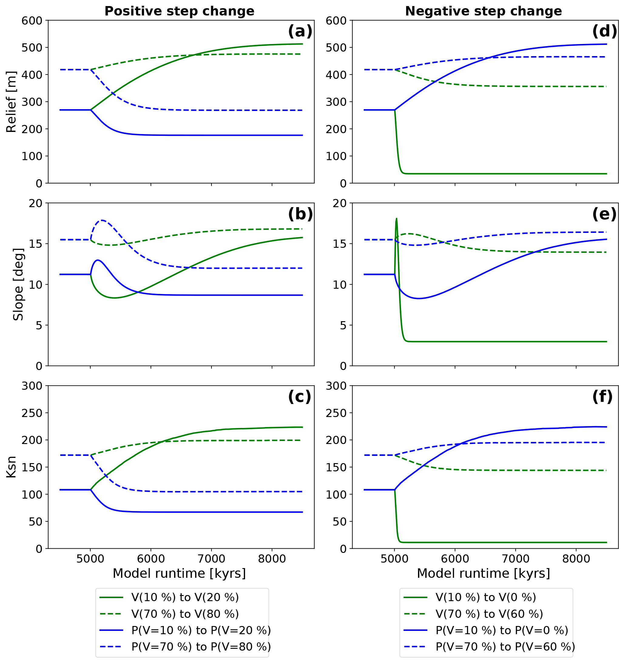
Figure 8 Observed evolution of topographic metrics after a step change in either vegetation (green lines) or mean annual precipitation (blue lines). Results are shown for two different initial vegetation cover amounts of V=10 and 70 %. Imposed mean annual precipitation changes were undertaken by selecting the precipitation amount corresponding to the initial and final vegetation amounts used in the simulations for vegetation cover “only” change. Panels (a), (b), and (c) show the reaction of model topographies to positive changes in boundary conditions. Panels (d), (e), and (f) show the reaction to negative changes in boundary conditions.

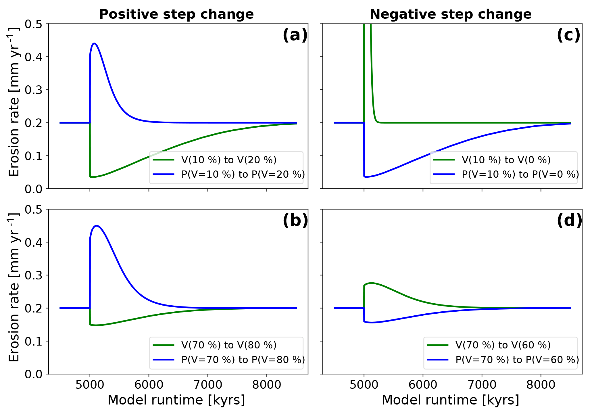
Figure 9 Mean catchment-wide erosion rates after a step-change disturbance in model boundary conditions. Blue lines represent erosion rates for models with changes in precipitation only; green lines represent erosion rates for models with changes in vegetation cover only. Panels (a) and (b) show the evolution after positive step change. Panels (c) and (d) show the evolution for models with negative step change. Note that the direction of change (positive or negative) from the initial state is in the opposite directions for precipitation and vegetation cover changes. This effect is manifested in the subsequent plots.

Although the above comparison between the models and the observations demonstrates a range of misfits between the two, there are several key points worth noting. First, the model results shown are simplified in their setup (e.g., assuming similar rock uplift rate and identical lithology and constants), and assume the present-day topography is in steady state for the comparison. Second, despite the previous simplifying assumptions, the degree of misfit between the observations and the model is surprisingly small when both vegetation and precipitation are considered (Fig. 7d, e, f). Finally (third), the general “hump-shaped” curve observed in the Chilean areas is captured in the model predictions (Fig. 7d, e, f), with the notable exception that the maximum in observed values occurs at a higher vegetation cover (V=70 %) than the model predictions (V=30 %). Explanations for the possible source of these differences are revisited in the discussion section of this paper.

4.2 Transient topography from a step change in vegetation or precipitation

The evolution of topographic metrics after an induced instantaneous disturbance (Fig. 4) of either only the surface vegetation cover (Fig. 8, green lines) or only the mean annual precipitation (Fig. 8, blue lines) is analyzed for changes in the topographic metrics for either a positive disturbance (Fig. 8a, b, c) or a negative disturbance (Fig. 8d, e, f). This scenario was chosen to analyze and isolate the effects of these specific transient forcings, and are useful for understanding the more complex changes in vegetation and precipitation presented later. Mean catchment erosion rates are also analyzed for their evolution after the disturbance (Fig. 9). For simplicity in presentation, results are shown for only two of the four Chilean study areas with initial vegetation (V) and precipitation (P) values for vegetation covers of 10 and 70 %, and precipitation rates that correspond to these vegetation covers (i.e., P(V=10 %) or P(V=70 %)) (Fig. 5). The results described below show a general positive correlation between all observed topographic metrics and surface vegetation cover, and a negative correlation between observed topographic metrics and mean annual precipitation.

4.2.1 Positive step change in vegetation cover or precipitation

Topographic analysis

A positive step change in vegetation cover (V) from V=10 % to V=20 % (solid green line Fig. 8a, b, c) leads to a factor of 1.9, 1.42, and 2.1 change in mean basin relief (from 270 to 520 m), mean basin slope (11.2 to 15.9^∘), and mean basin channel steepness (108 to 222 m^−0.9), respectively. The adjustment time until a new steady state in each metric is reached is 3.1 Ma. The corresponding positive change in mean annual precipitation (solid blue lines, Fig. 8a, b, c) leads to a decrease of the mean basin relief to 176 m, the mean basin slope to 8.6^∘ and the mean basin channel steepness to 67 m^−0.9. This corresponds to a decrease by factors of 1.5, 1.2, and 1.6, respectively. The adjustment time to new steady-state conditions in this case is shorter and was found to be 1.1 Ma (Fig. 8a, b, c). A second feature of these results is the brief increase and then decrease in basin average slope angles following the step change (Fig. 8b).

For simulations with V=70 % initial surface vegetation cover, a positive increase to V=80 % leads to an increase of the mean basin relief from 418 to 474 m, the mean basin slope from 15.5 to 16.8^∘, and the mean basin channel steepness from 172 to 199 m^−0.9. This causes an increase in each metric by a factor of 1.1, 1.1, and 1.2, respectively. The adjustment time to steady-state conditions is 1.9 Ma (dotted green lines, Fig. 8a, b, c). The corresponding positive change in mean annual precipitation leads to a decrease of relief to 268 m, a decrease in slope to 11.9^∘, and a decrease of channel steepness to 105 m^−0.9. This resembles a decrease by factors of 1.5, 1.3, and 1.6, respectively. Adjustment time in this case is 1.7 Ma (dotted blue lines, Fig. 8a, b, c). The basin slope data show similar behavior as the V_ini=10 % simulations with an initial decrease and subsequent increase for a vegetation cover step change, and an initial increase and subsequent decrease for a step change in mean annual precipitation. A comparison of the change in the topographic metrics for the low (V=10 %) and high (V=70 %) initial vegetation covers, shows that the magnitude of change in each metric is larger when the step change occurs on a low, rather than a higher, initial vegetation cover topography.

Erosion rate changes

The model results show a negative relationship between increases in vegetation cover and erosion and a positive relationship between increases in precipitation and erosion (Fig. 9). Although the response between the disturbances and changes in erosion rates are instantaneous, the maximum or minimum in the change is reached after some lag time, and the magnitude and duration of nonequilibrium erosion rates varies between different simulation setups.

For an initial vegetation cover of V=10 %, a change in vegetation cover (dV) of +10 % leads to a decrease in erosion rates from 0.2 to 0.03 mm yr⁻¹ (a factor of 5.7 decrease, Fig. 9a green line). The minimum erosion rate is reached 43.5 kyr after the step change occurs. Following this minimum in erosion rates, the rates increase until the steady-state erosion rate is reached after the adjustment time. An increase in mean annual precipitation, corresponding to a vegetation cover of 10 % (i.e., P(V=10 %) to P(V=20 %); Fig. 5), leads to an increase in erosion rates to a maximum of 0.44 mm yr⁻¹ after 74.8 kyr (a factor of 2.2 increase, Fig. 9a, blue line). For an initial vegetation cover of V=70 %, a vegetation increase of dV $=+\mathrm{10}$ % results in minimum erosion rates of 0.14 mm yr⁻¹ after 117.7 kyr (a factor of 1.4 decrease, Fig. 9b, green line). A corresponding increase in precipitation for these same vegetation conditions leads to maximum erosion rates of 0.44 mm yr⁻¹ after 107.5 kyr, which is an increase by a factor of 2.2 (Fig. 9b, blue line). The previous results for a positive step change in vegetation or precipitation demonstrate that the magnitude of the change in erosion rates is larger for changes in precipitation rate than for vegetation cover changes; furthermore, in low initial vegetation cover settings (V=10 %) the magnitude of the change in erosion rates for changing vegetation is larger (compare green lines Fig. 9a with b).

4.2.2 Negative step change in vegetation cover or precipitation

Topographic analysis

For negative step changes in vegetation (green curves, Fig. 8d, e, f), the results show a sharp decrease in the topographic metrics associated with shorter adjustment times compared to the positive step change experiments (compare Fig. 8d, e, f with a, b, c). For step changes in precipitation (blue curves, Fig. 8d, e, f), the increase of topographic metrics happens slower, which equates to longer adjustment times. A negative step change in vegetation cover from V=10 % by dV $=-\mathrm{10}$ % leads to a decrease of the mean basin relief from 269 to 35 m, the mean basin slope from 11.2 to 2.3^∘, and the mean basin channel steepness from 108 to 11 m^−0.9, which resembles decreases by factors of 7.8, 3.8, and 9.6, respectively. The adjustment time until a new steady state is reached is 0.26 Ma (solid green lines, Fig. 8d, e, f). The corresponding negative change in precipitation leads to an increase in the mean basin relief to 512 m, the mean basin slope to 15.8^∘, and the mean basin channel steepness to 223 m^−0.9. These increases reflect changes by factors of 1.9, 1.4, and 2.1, respectively, with an adjustment time of 4.9 Ma (dotted green lines, Fig. 8d, e, f). Mean basin slope results (Fig. 8e) for a step change in vegetation illustrate a pulse-like feature of initially increasing slope values, followed by a decrease to lower slope values. In contrast, a negative step change in precipitation induces an initial decrease in slope, followed by a gradual increase in slope to a value higher than was initially observed before the change.

Simulations with initial vegetation cover of V=70 % and dV $=-\mathrm{10}$ % show a decrease in the mean basin relief from 418 to 356 m, the mean basin slope from 15.5 to 13.6^∘, and the mean basin channel steepness from 172 to 144 m^−0.9, which resembles changes by respective factors of 1.2, 1.1, and 1.2 and an adjustment time of 2.1 Ma (dotted green lines, Fig. 8d, e, f). Corresponding negative changes in precipitation lead to increase of the basin relief of 465 m, the basin slope to 16.4^∘, and the channel steepness to 195 m^−0.9, which resembles changes by factors of 1.1 for all three values. Adjustment time in this case is 2.2 Ma (dotted blue lines, Fig. 8d, e, f). Behavior of mean basin slope after the step change follows the V=10 % simulations, but shows lower amplitudes of basin slope for both step changes in vegetation and precipitation.

Erosion rates

The positive step-change results (Fig. 9a, b) indicated that erosion rates reach their minimum or maximum with a lag time. The results also show significant differences in the magnitude and duration of nonequilibrium conditions depending on if vegetation or precipitation were changing. Simulations with a decrease from V=10 % to V=0 % (Fig. 9c) show a sudden increase in erosion rates to a maximum value of 3.5 mm yr⁻¹, which is an increase from steady-state conditions by a factor of 17.7. This value is reached after 19.5 kyr (green line, Fig. 9c). A step decrease in precipitation for this corresponding vegetation difference (i.e., P(V=10 %) to P(V=0 %) leads to a smaller, and protracted (longer adjustment time) decrease in erosion rates to 0.03 mm yr⁻¹ after 50.1 kyr. These conditions cause a factor of 5.6 decrease (blue line, Fig. 9c). Simulations of V=70 % with a vegetation change of dV $=-\mathrm{10}$ % show an increase in erosion rates to 0.27 mm yr⁻¹, which is a factor of 1.4 increase after 126.3 kyr (Fig. 9d). For the corresponding decrease in precipitation the data show a decrease in erosion rates to 0.15 mm yr⁻¹ after 124.5 kyr. This resembles change by factor of 1.2 (blue line, Fig. 9d).

4.3 Transient topography – oscillating

4.3.1 Oscillating surface vegetation cover and constant precipitation

Topographic analysis

The topographic evolution in simulations with a constant precipitation (10 and 360 mm yr⁻¹ for V=10 % and V=70 %, respectively) and oscillating vegetation cover show a different response than the previous step change experiments. The differences depend on the initial steady-state vegetation cover prior to the onset of 100 kyr oscillations. All observed basin metrics (Fig. 10) show an initial oscillating decrease in values until a new dynamic steady state is reached where the amplitude in oscillations is less than in the preceding initial adjustment period. Simulations with V=10 % (Fig. 10a) show a factor of 2.5 decline in the basin relief (from 269 to 107 m). For simulations with V=70 % the reaction and adjustment to the new dynamic steady state is less pronounced with a factor of 1.01 decline in relief (from 410 to 407 m), and positive and negative amplitudes in the dynamic steady state of 1.6 m. While these changes are unmeasurable in reality, they highlight that changes in vegetation cover alone would be difficult to detect for high initial vegetation cover settings. The analysis of the mean basin slope for the model topographies with low (V=10 %) vegetation shows a similar behavior with a factor of 1.6 decrease of the mean slope (from 11.2^∘ prior to the onset of oscillations, to 6.0^∘, Fig. 10b). However, before this new equilibrium is reached, the slopes show an increase in the mean slope for the first two periods of vegetation oscillation, which then declines towards the new long-term stable dynamic equilibrium. This equilibrium is reached after approximately 500 kyr. Local maxima of the mean basin slope coincide with local minima in basin relief. For the V=70 % simulations, the reaction is significantly smaller with no change in mean slope for the new dynamic equilibrium and both positive and negative amplitudes of 0.16^∘. Mean basin channel steepness (Fig. 10c) reflects the behavior of mean basin elevation. For V=10 % simulations the mean channel steepness decreases by a factor of 2.7 (from 108 to 40 m^−0.9) with a positive amplitude of 3.7 m^−0.9 and a negative amplitude of 6.1 m^−0.9. For V=70 % simulations the response is again only minor, compared to the lower initial vegetation cover simulations with a change of mean channel steepness from 186 to 167 m^−0.9, positive amplitudes of 1.1 m^−0.9, and negative amplitudes of 0.9 m^−0.9. Like the elevation data, the steepness data show a distinct oscillating pattern with a slow increase to local maxima and rapid decrease to local minima, which coincide with maxima/minima of elevation data. Taken together, the previous observations demonstrate a larger change in topography for oscillations in poorly vegetated areas compared to those with higher vegetation cover. Furthermore, the magnitude of topographic change that oscillations in vegetation impose on topography are largest in the first ∼500 kyr after the onset of an oscillation, and diminish thereafter.

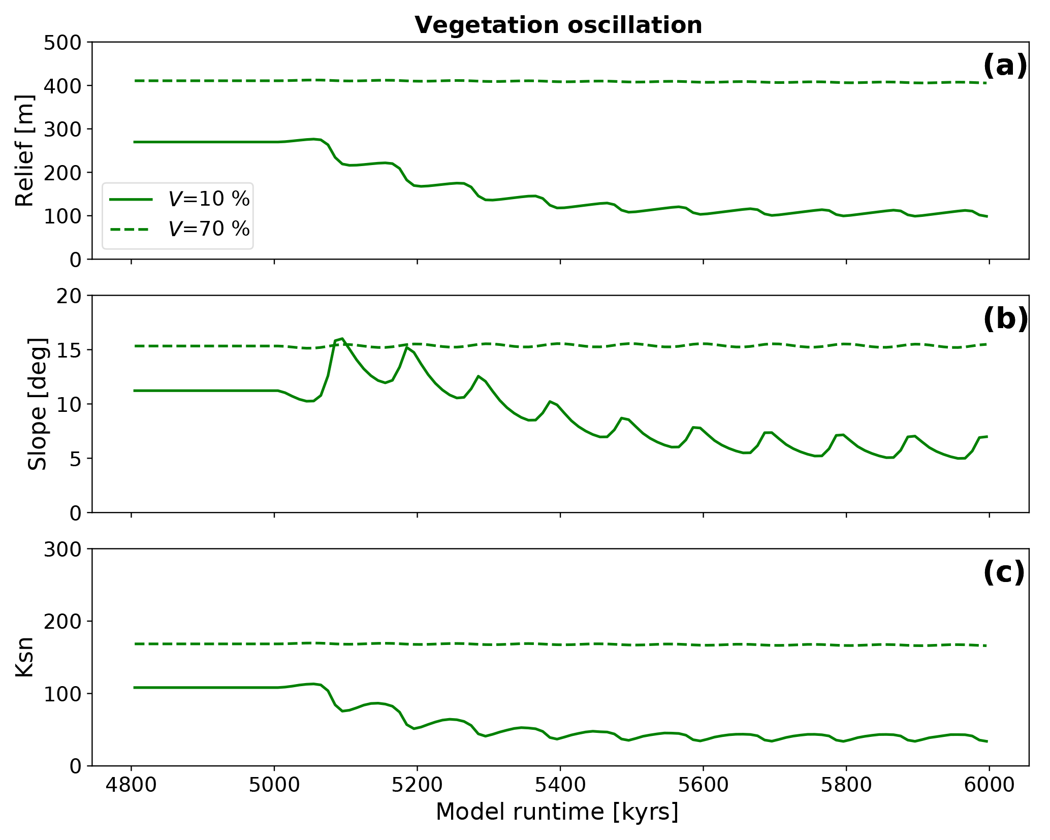
Figure 10 Evolution of topographic metrics for simulations with oscillating surface vegetation cover and constant precipitation corresponding to the initial vegetation cover prior to the transient in vegetation cover. Panels a, b, and c show the mean basin relief, the mean basin slope, and the mean basin channel steepness (K_sn), respectively.

Erosion rates

The erosion history for simulations with oscillating vegetation cover (Fig. 11) demonstrate large variations in the erosion rate that depend on the average vegetation cover of the oscillation. Furthermore, pronounced differences in the amplitude of erosion occur if the vegetation cover is above or below the mean of the oscillation (Fig. 4a). More specifically, simulations with V=10 % show a pattern of a small decrease in erosion rates (from 0.2 to 0.03 mm yr⁻¹) when vegetation cover increases above the mean cover, in contrast to a large increase in erosion rates (up to 3.3 mm yr⁻¹) when vegetation cover decreases below the mean of the oscillation (Figs. 2, 11). Maximum erosion rates decline over multiple periods of oscillation until they reach a dynamic steady state with maximum rates (1.2 mm yr⁻¹) at 760 kyr after the onset. Time periods of higher erosion rates (> 0.2 mm yr⁻¹) have a mean duration of 28 kyr, whereas periods of lower erosion rates (< 0.2 mm yr⁻¹) have a mean duration of 72 kyr. For simulations with high vegetation cover (V=70 %) the maximum and minimum erosion rates are 0.28 and 0.15 mm yr⁻¹, respectively. The magnitude of maximum and minimum erosion rates are not significantly time-dependent, meaning that they are constant over the simulation. The mean duration of periods with higher erosion rates (> 0.2 mm yr⁻¹) is 55 kyr, whereas the duration for periods with lower rates (< 0.2 mm yr⁻¹) is 45 kyr. These results demonstrate that areas with low vegetation cover experience not only larger amplitudes of change in erosion rates, but also an asymmetric change whereby decreases in erosion rates are of a lower magnitude than the increases in erosion rates.

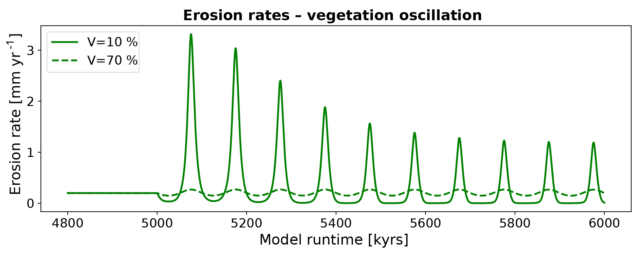
Figure 11 Predicted mean catchment erosion rates for simulations with oscillating surface vegetation cover and constant precipitation. Note that the magnitude of change in erosion rates for a ±10 % change in vegetation cover differs depending on the initial (or background) vegetation cover. This nonlinear response is due, in part, to the vegetation cover effects on rock erodibility and diffusivity shown in Fig. 6.

4.3.2 Oscillating precipitation and constant vegetation

Topographic analysis

The evolution of topographic parameters for simulations with oscillating mean annual precipitation and two different constant surface vegetation covers (V=10 or 70 %, Fig. 12) shows a less extreme and smaller temporal change in erosion rate to variations in precipitation compared to the previously discussed effects of oscillating vegetation cover (Fig. 11). In Fig. 12a, the mean basin relief results for V=10 % and oscillating precipitation show small variations (+4.9 to −3.8 m) in relief around a mean of 269 m, which is similar to the mean relief prior to the onset of oscillations at 5000 kyr. For simulations with V=70 % the change in relief is slightly more pronounced with factor of 1.1 adjustment to a new mean (380 from 418 m) in steady-state conditions. The evolution of the topographic slope (Fig. 12b) for V=10 % simulations shows a factor of 1.05 adjustment to a new dynamic equilibrium (from 11.2 to 10.6^∘). For V=70 % the mean slope values do not significantly change from steady-state to transient conditions. Mean channel steepness (Fig. 12c) for V=10 % shows a factor of 1.01 adjustment (from 108 to 110 m^−0.9), and would be difficult to measure in reality. The amplitude of oscillation is 4 m^−0.9 for both negative and positive amplitudes. For V_ini=70 % simulations, a factor 1.1 change in channel steepness occurs (from 171 to 152 m^−0.9) with amplitudes of 4.5 m^−0.9 for both positive and negative changes. Figure 12 illustrates changes in topographic metrics that result from oscillations in precipitation occurring around vegetation covers of 10 and 70 %. These changes are significantly smaller than those predicted for constant precipitation with oscillating vegetation conditions (Fig. 10).

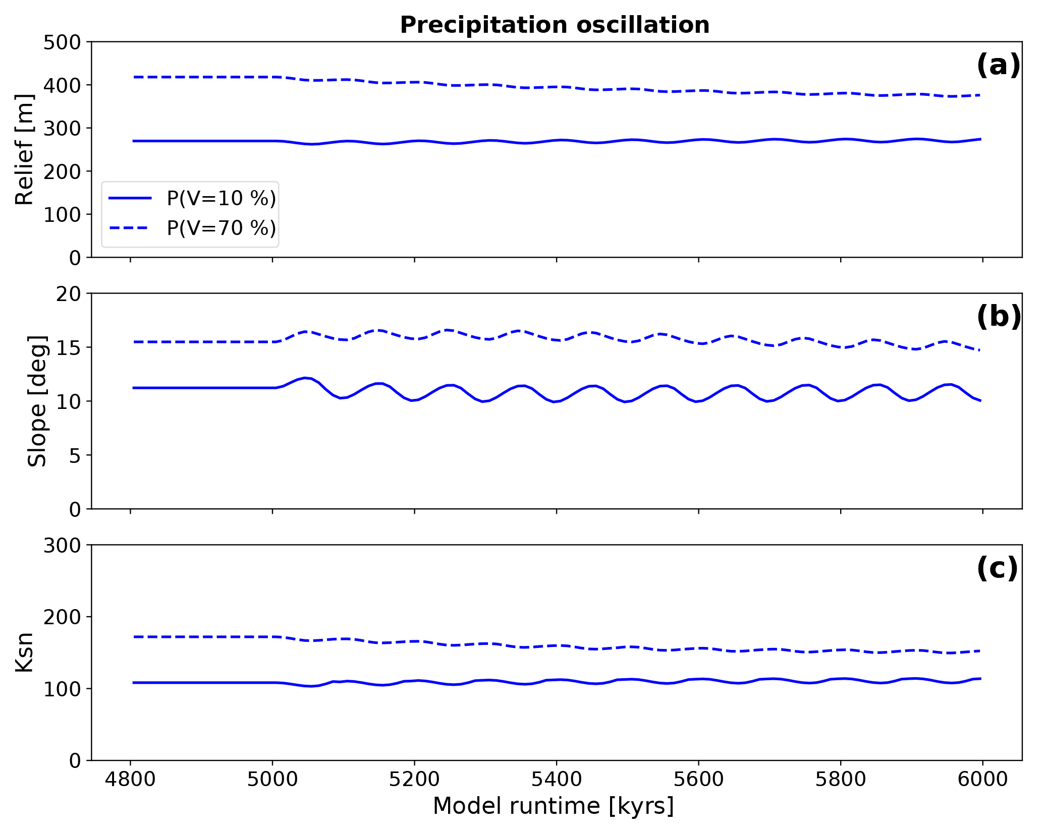
Figure 12 Evolution of topographic metrics for simulations with oscillating mean annual precipitation and constant vegetation cover. The vegetation cover was held constant at the value corresponding to the precipitation rate prior to the onset of the transient at 5000 kyr. Panels (a), (b), and (c) show the mean basin relief, the mean basin slope, and the mean basin channel steepness (K_sn), respectively.

Erosion rates

Predicted erosion rates from simulations with constant surface vegetation cover and oscillating mean annual precipitation indicate different amplitudes of change around the mean erosion rate depending on the vegetation cover. For simulations with V=10 % (Fig. 13, blue solid line) erosion rates oscillate symmetrically around the steady-state erosion rate (0.2 mm yr⁻¹). The maximum and minimum erosion rates of 0.42 and 0.01 mm yr⁻¹, respectively, do not lead to a shift in the mean value of erosion rates over time. In contrast, predicted rates with a higher vegetation cover of V=70 % (Fig. 13, blue dotted line) demonstrate an asymmetric oscillation in rates around the mean, whereby the maximum rates (0.43 mm yr⁻¹) have a larger difference above the mean rate than the minimums in the oscillation do (0.12 mm yr⁻¹). For this higher vegetation cover scenario, a gradual decrease in the mean erosion rate occurs as time progresses. Furthermore, the maximum and minimum erosion rates decline over several oscillation periods. Taken together, these results indicate that oscillations in precipitation impact erosion, with the magnitude of the effect depending on the amount of vegetation cover. Areas with low vegetation cover demonstrate the highest and most symmetric oscillation of erosion rates due to changes in precipitation, whereas in areas with high vegetation cover the effect of negative changes in precipitation is dampened by vegetation.

5 Discussion

The previous results highlight different sensitivities to changes in either surface vegetation cover or mean annual precipitation. In the following, we synthesize the previous results and then build upon them to discuss the scenario of synchronous variation in both precipitation and vegetation cover.

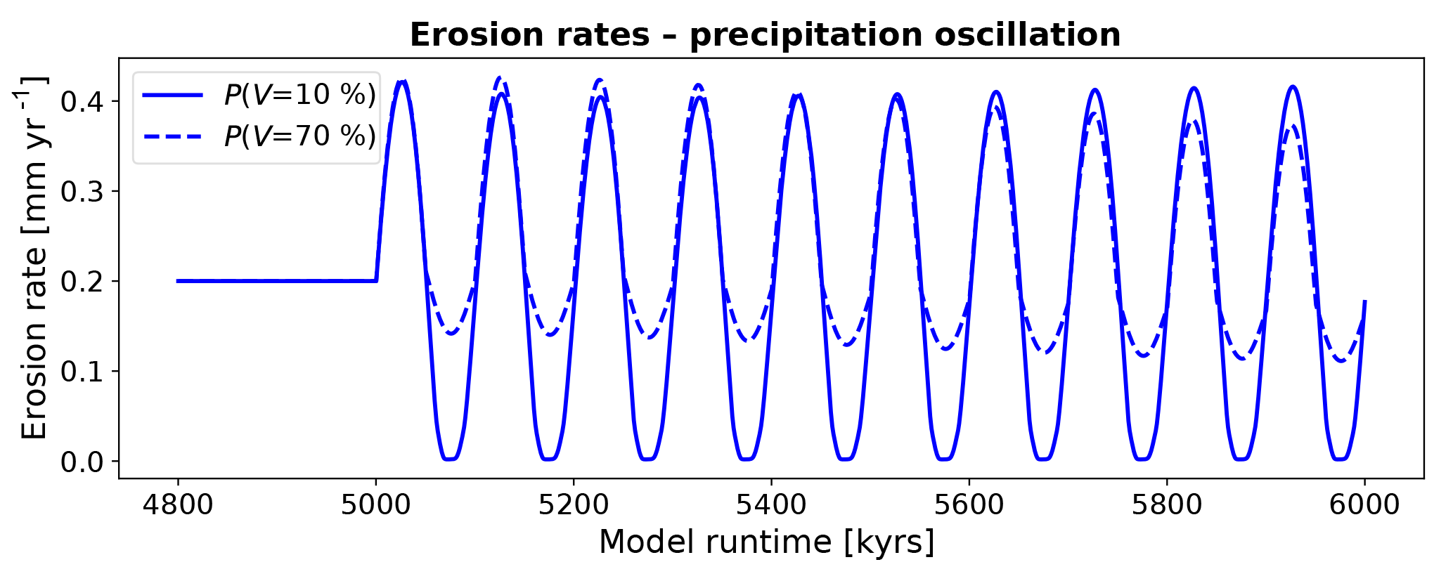
Figure 13 Mean catchment erosion rates for simulations with oscillating mean annual precipitation and constant surface vegetation cover. The amplitude of change in the erosion rates varies with the initial vegetation cover, in part due to the nonlinear relationship between precipitation and vegetation cover (Figs. 4, 5).

5.1 Interpretation of steady-state simulations

Landscapes in a topographic steady state show distinct features in topographic metrics that are widely used to estimate catchment-averaged erosion rates and the related leading processes of erosion within a landscape (DiBiase et al., 2010). The steady-state simulations presented here can reproduce (Fig. 7) variations in topographic metrics over different climate and vegetation states than those seen in other studies (Langbein and Schumm, 1958; Walling and Webb, 1983). The comparison of simulations with homogeneous precipitation and changing values of vegetation cover (Fig. 7a, b, c) to simulations with both changing precipitation and vegetation cover values (Fig. 7d, e, f), indicates that we can only reproduce a similar trend with a distinct peak in topographic metrics when both precipitation and vegetation cover variables are considered. From this, we conclude that modern model-based landscape evolution studies, which aim to compare areas with different climates, should incorporate vegetation dynamics in their simulations. Misfits between the predicted and Chilean observed topographic metrics (Fig. 7d, e, f), present when the vegetation and precipitation both vary, likely stem from the simplicity of the model setup used and the likelihood of differences in the rock uplift rate and lithologies present in these areas.

5.2 Interpretation of step change experiments

Our analysis shows that changes in vegetation cover typically have a higher magnitude of impact on topographies for lower values of initial vegetation cover, compared to simulations with high initial vegetation cover (Figs. 8, 9). In these settings the influence of vegetation cover outweighs the influence of precipitation regarding cases of negative and positive directions of the step change. The reason for this is the higher impact of changes in vegetation than the impact of changes in precipitation on erosivity and diffusivity (parameter K_v, K_d; Eqs. 4, 10).

Furthermore, a negative step change in vegetation cover impacts the topographic metrics by a factor of 2 more than positive step change changes do (Fig. 8d, e, f). This response is interpreted to be due to the nonlinear reaction of diffusivity and fluvial erodibility to changes in vegetation cover (See Fig. 6). Negative changes in vegetation cover lead to a higher overall change in diffusivity and erodibility compared to positive step changes.

Model results for the topographic metrics and erosion rates also indicate a difference in the adjustment times of the system until a new steady state is reached when either precipitation or vegetation cover changes (Figs. 8, 9). For simulations with positive step changes (Fig. 8a, b, c) the adjustment time for changes in vegetation cover to reach a new equilibrium in topographic metrics or erosion rates is 3 times longer than the adjustment time for changes in precipitation. Simulations with negative step changes in vegetation cover show an adjustment time that is shorter by a factor of 18 compared to negative changes in precipitation. This difference in adjustment time is again a result of the nonlinear behavior of erosion parameters K_d and K_v, which influence how effectively a signal of increasing or decreasing erosion can travel through a river basin (Perron et al., 2012). High values of K_d and K_v are associated with lower adjustment times and are a result of negative changes in vegetation cover. The influence of changing precipitation on adjustment time behaves in a more linear fashion; therefore, it mostly depends on the overall magnitude of change. Thus, positive step changes in vegetation cover decrease K_d and K_v, which leads to higher adjustment times than the corresponding changes in precipitation.

An increase and subsequent decrease, or decrease and subsequent increase, in predicted slope and erosion rates is observed for both the positive and negative step change experiments (Figs. 8b, e and 9). This nonlinear response in both positive and negative step changes in precipitation and vegetation cover is also manifested in the subsequent oscillation experiments, although it is most clearly identifiable in the step change experiments. The explanation for this behavior is as follows. A positive step change in vegetation cover (Fig. 8b) leads to a decrease in fluvial capacity, as increased vegetation cover increases the Manning roughness (parameter n_v, Eq. 8). The effect of changing the Manning roughness varies with the location within the catchment, and influences which processes (fluvial or hillslope) most strongly impact slopes and erosion rates. In the upper part of catchments, where contributing areas (and discharge) are low, this increase in Manning roughness causes many areas to be below threshold conditions; therefore, fluvial erosion is less efficient, and hillslope diffusion increases in importance and reduces slopes. In the lower part of catchments, where contributing area and discharge are higher, changes in the Manning roughness are not large enough to impact fluvial erosion because these areas remain at, or above, threshold conditions for erosion. With time, the lower regions of the catchments that are at or above threshold conditions propagate a wave of erosion up to the higher regions that are below threshold conditions. This propagating wave of erosion eventually leads to an increase in slope angles, which is essential due to the response time of the fluvial network to adjust to the new Manning roughness conditions.

In contrast, a positive step change in mean annual precipitation leads to an initial increase in fluvial shear stress, which initially causes headward incision of river channels and leads to a wave of erosion that propagates upstream and increases channel slope values (Fig. 8b, see also e.g., Bonnet and Crave, 2003). The increase in channel slopes leads to an increase in the hillslope diffusive flux adjacent to the channels that then propagates upslope. Eventually, this increase in the hillslope flux leads to a decrease in hillslope angles, and an overall reduction in mean catchment slopes after the systems reaches equilibrium.

Negative step changes in vegetation cover or precipitation (Fig. 8e, green curves) show the opposite behavior to the previous positive step change description. A negative step change in vegetation cover leads to an initial increase of fluvial erosion throughout the catchment, as the Manning roughness decreases everywhere. This catchment-wide decrease in Manning roughness leads to fluvial incision throughout the catchment and an increase in mean slope. However, eventually hillslope processes catch up with increased slopes near the channels, and with time an overall reduction of slope occurs. Negative changes in precipitation (Fig. 8e, blue curves) lead to an initial decrease in fluvial erosion, thereby leading to an increase in the significance of hillslope processes such that slope angles between channels and ridges decrease as hillslope processes fill in channels. With time, the fluvial network equilibrates to lower precipitation conditions by increasing slopes to maintain equilibrium between erosion and rock uplift rates.

Thus, the contrasting behavior of either initially increasing or decreasing slopes and erosion rates, followed by a change in the opposite direction of this initial change, highlight a complicated vegetation–climate induced response to changes in either parameter. This nonlinear behavior, and the millennial timescales over which these changes occur, suggest that modern systems that have experienced past changes in climate and vegetation will likely be in a state of transience; therefore, the concept of a dynamic equilibrium in hillslope angles and erosion rates may be difficult to achieve in these natural systems.

Previous studies have inferred relationships between mean catchment erosion rates derived from cosmogenic radionuclides and topographic metrics (e.g., DiBiase et al., 2010; DiBiase and Whipple, 2011). However, the previous discussion of how topographic metrics change in response to variable precipitation and vegetation suggests that empirical relationships between erosion rates and topographic metrics contain a signal of climate and vegetation cover in the catchment. We illustrate the effect of step changes in climate and vegetation on the new steady state of topographic metrics in Fig. 14. In this example, the new steady-state conditions in basin relief and mean slope after a modest (±10 %) change in vegetation or precipitation (triangles) differ from the initial steady-state condition (circles). These changes in topographic metrics when the new steady state is achieved occur despite the rock uplift rate remaining constant.

5.3 Interpretation of oscillation experiments

The results from the 100 kyr oscillating vegetation and precipitation conditions show that oscillating vegetation cover without the corresponding oscillations in precipitation leads to adjustments of topographic features, which results in a new dynamic equilibrium after approximately 1.5 Ma (Figs. 10, 11). The previously described response of topographic metrics and erosion rates to oscillating vegetation (see results section) are due to processes described in the previous step change experiments. For example, the asymmetric oscillations in topographic metrics for V=10 % (Fig. 10) are due to the superposition of the positive, and subsequent negative, changes described in Sect. 5.2. Variations in the imposed Manning roughness, and the relative strengths of fluvial vs. hillslope processes in different parts of the catchments at different times cause the topographic metrics and erosion rates to have variable amplitudes and shapes of response due to the symmetric oscillations imposed on the topography (Fig. 4a).

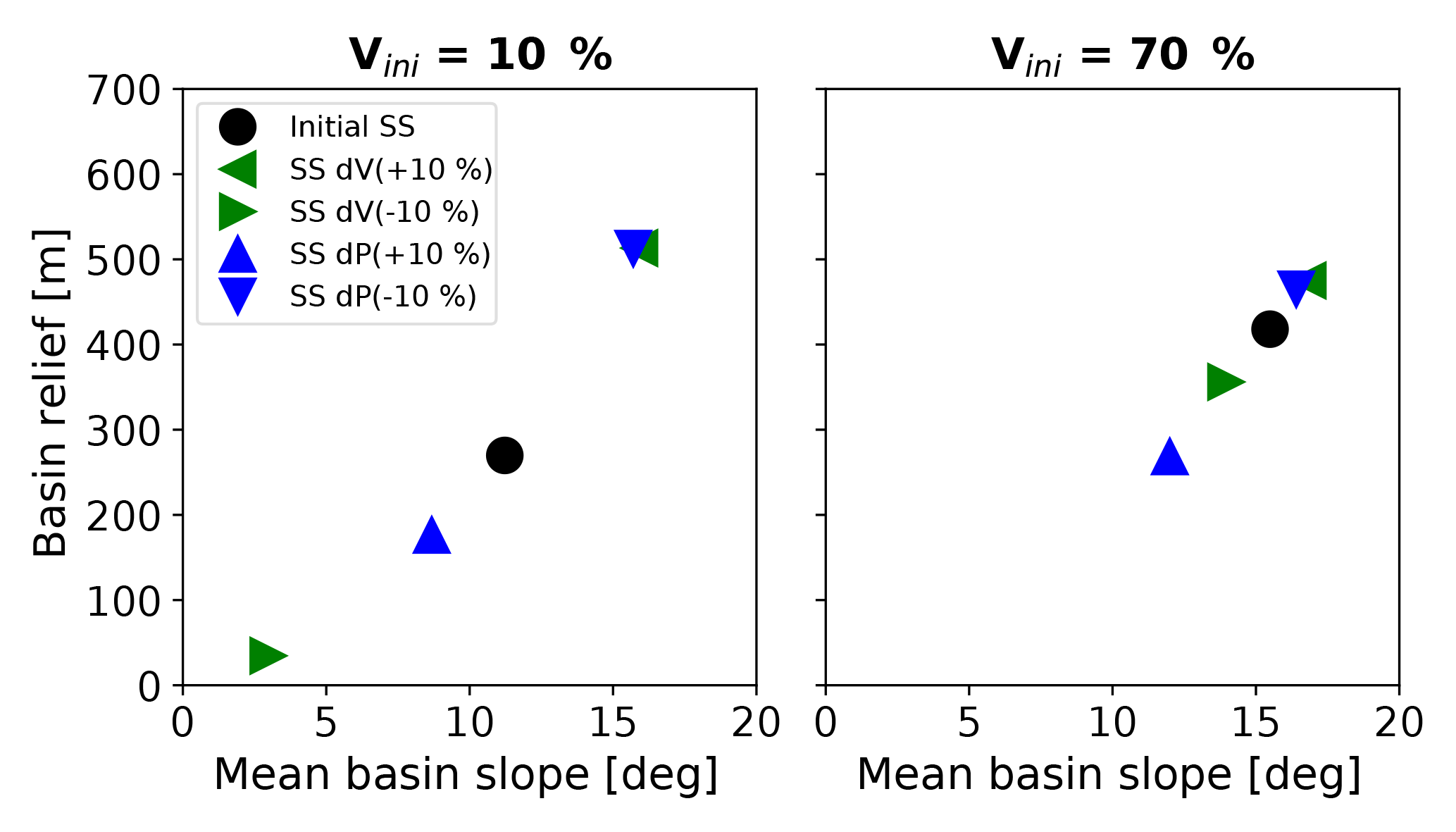
Figure 14 Shifts in the mean basin slope–mean basin relief relationship for simulations with positive and negative step changes in either vegetation cover (green triangles) or mean annual precipitation (blue triangles). Black dots represent initial steady-state conditions prior to any imposed transient in vegetation cover or mean annual precipitation. Note that the sensitivity of topographic relief to perturbations in precipitation or vegetation cover is highest for low vegetation cover (10 %) settings.

Simulations with oscillating precipitation and constant vegetation cover show a less pronounced shift to new equilibrium conditions and lower amplitudes of oscillation in both topographic metrics and erosion (Figs. 12, 13). This difference in the response of the topographic metrics and erosion rates shown in Figs. 12 and 13, compared to the oscillating vegetation cover experiments (Figs. 10, 11), is due to the higher impact of changes in vegetation cover on parameters that guide erosion rates and the related adjustment to topographic metrics compared to the corresponding changes in precipitation in our model domains (Fig. 5). Especially for simulations with low initial vegetation cover, the effect of changing vegetation has a larger magnitude of effects due to the nonlinear response of diffusivity and fluvial erodibility to changes in vegetation cover compared to the linear response to changes in precipitation.

5.4 Coupled oscillations in both vegetation and precipitation

The previous sections present a sensitivity analysis of how step changes or oscillations in either vegetation cover or precipitation influence topography. Here we present a step-wise increase towards reality by investigating the topographic response to changes in both precipitation and climate at the same time. The amplitude of change prescribed for both precipitation and vegetation is based upon the present empirical relationship observed in the Chilean study areas for initial vegetation covers of 10 and 70 %, and mean annual precipitations of 10 and 360 mm yr⁻¹ (Fig. 5). As with the previous experiments, oscillations in parameters were imposed upon steady-state topography that was developed with the previous values, and a rock uplift rate of 0.2 mm yr⁻¹.

Figure 15 shows the evolution of topographic metrics for simulations with combined oscillations in precipitation and vegetation. The variation in topographic metrics resembles those described for simulations with constant vegetation cover and oscillating climate by showing little to no significant adjustment towards new dynamic steady-state conditions. The amplitudes of oscillation are dampened from those of previous results because of the opposing effects of changes in precipitation and vegetation cover (e.g., compare blue and green curves in Figs. 8 and 9).

However, inspection of the predicted erosion rates (Fig. 16) for the combined oscillations indicates a significant (∼0.1 – ∼0.15 mm yr⁻¹), and highly nonlinear, response. The response between the 70 % and 10 % vegetation cover scenarios are very different. For heavily vegetated areas (P(V=70 %)) erosion rates typically increase during an oscillation, whereas for the low vegetation cover conditions (P(V=10 %)) erosion rates initially show a decrease and then increase and decrease at a higher frequency.

To better understand this contrast in the response to combined precipitation and vegetation changes, the first 100 kyr cycle is shown in Fig. 17. After an oscillation starts, the 10 % initial vegetation cover simulations show a decline in erosion rates with the minimum erosion rate correlated with the highest values of both vegetation cover and mean annual precipitation (compare top and bottom panels). This part of the response is interpreted as resulting from the hindering effect of increased vegetation on erosion rates outweighing the impact of higher precipitation on erosion rates because vegetation decreases the effectiveness of erosion and transport of surface material (Fig. 17). After values of vegetation cover and precipitation start to decline, erosion rates show a very rapid increase to values of ∼0.3 mm yr⁻¹. This increase in erosion rates is due to an increase in both K_v and K_d (Fig. 3b, Eqs. 4, 5), which outcompetes the effect of precipitation decrease.

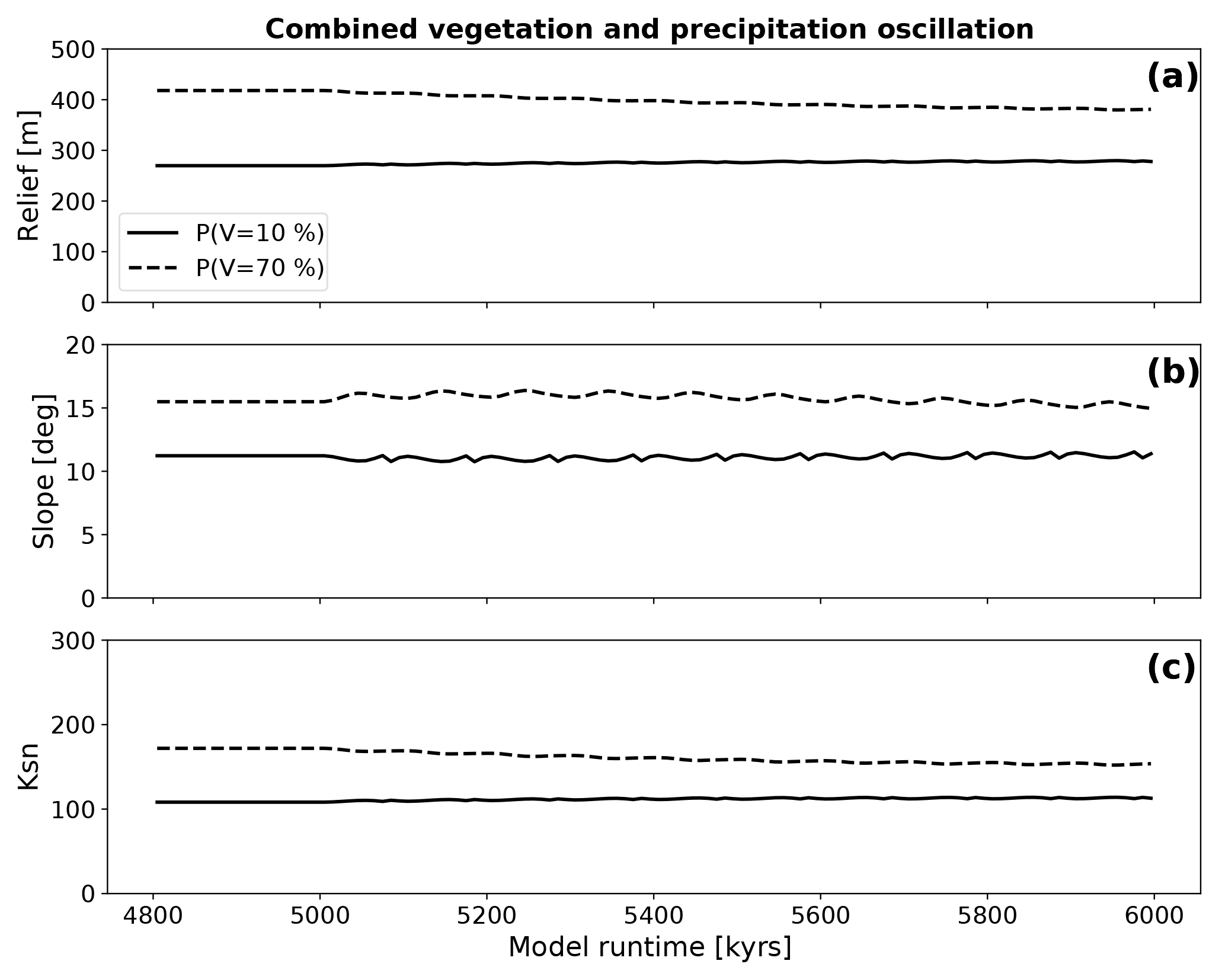
Figure 15 Evolution of topographic metrics for coupled simulations where both changes in surface vegetation cover and a corresponding change in mean annual precipitation (Fig. 5) are simultaneously imposed. The amplitudes and frequency of the forcings that were imposed on the simulations are the same as those used for the simulations with isolated transient forcings. Panels (a), (b), and (c) show the evolution of the mean basin relief, the mean basin slope, and the mean basin channel steepness (K_sn) after the start of the oscillation at 5 Ma. Note the muted/damped response relative to previous simulations of oscillating vegetation cover or precipitation conditions.

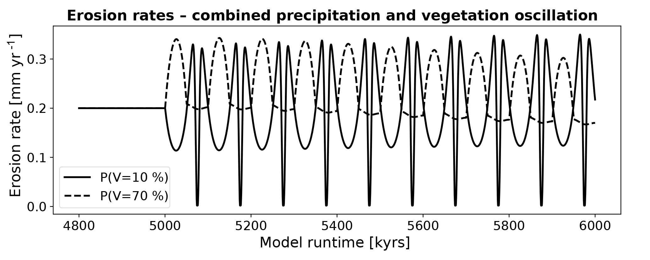
Figure 16 Mean catchment erosion rates for coupled simulations with changes in surface vegetation cover and mean annual precipitation. The first cycle in the time series is expanded in Fig. 17. The variable amplitude and nonlinear response shown here is due to the combined nonlinear forcings in precipitation (Figs. 4, 5) and rock erodibility and diffusivity (Fig. 6) for different initial vegetation cover amounts.

Following this, a sudden drop in erosion rates occurs (to 0 mm yr⁻¹) and lasts for 3 kyr due to the onset of hyper-arid conditions at minimum precipitation. After this low in erosion rates, they once again increase (to 0.3 mm yr⁻¹) as precipitation and vegetation cover increase, while the effect of increased precipitation outweighs the effect of the nonlinear decrease in K_v and K_d (Fig. 3b, c; Eqs. 4, 5). Finally, at the end of this complex cycle a decrease in erosion rates occurs (Fig. 17b), while vegetation and precipitation are increasing (upper panel) because the effect of vegetation increases K_v∕K_d and outweighs the effect of increasing precipitation.

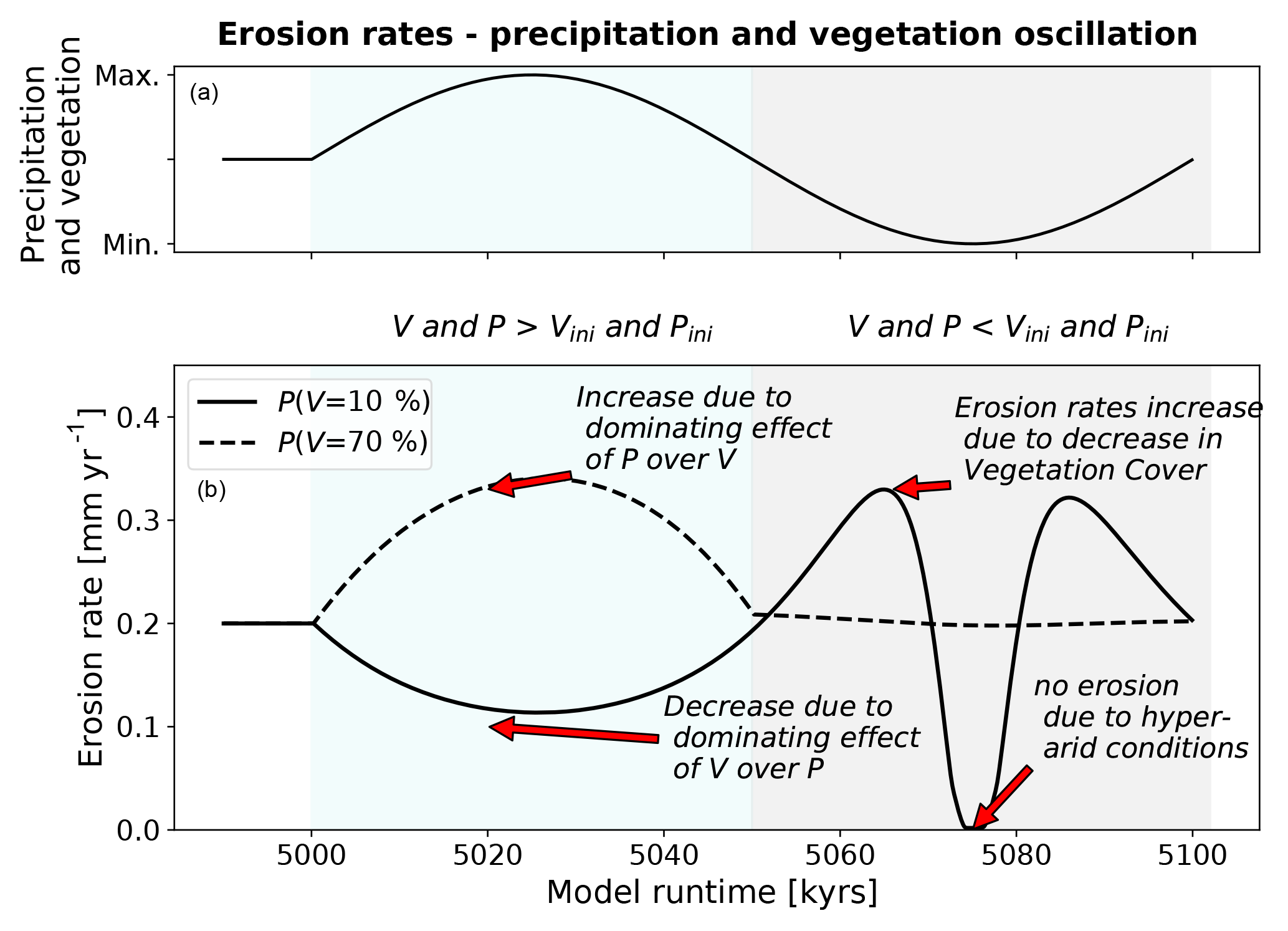
Figure 17 Mean catchment erosion rates for coupled simulations for one period of oscillation after the start of transient conditions (see also Fig. 15). Panel (a) shows conceptualized transient forcing in vegetation cover and mean annual precipitation. Panel (b) shows the erosion rates for simulations with low (black line) and high (dotted line) initial vegetation cover and precipitation values.

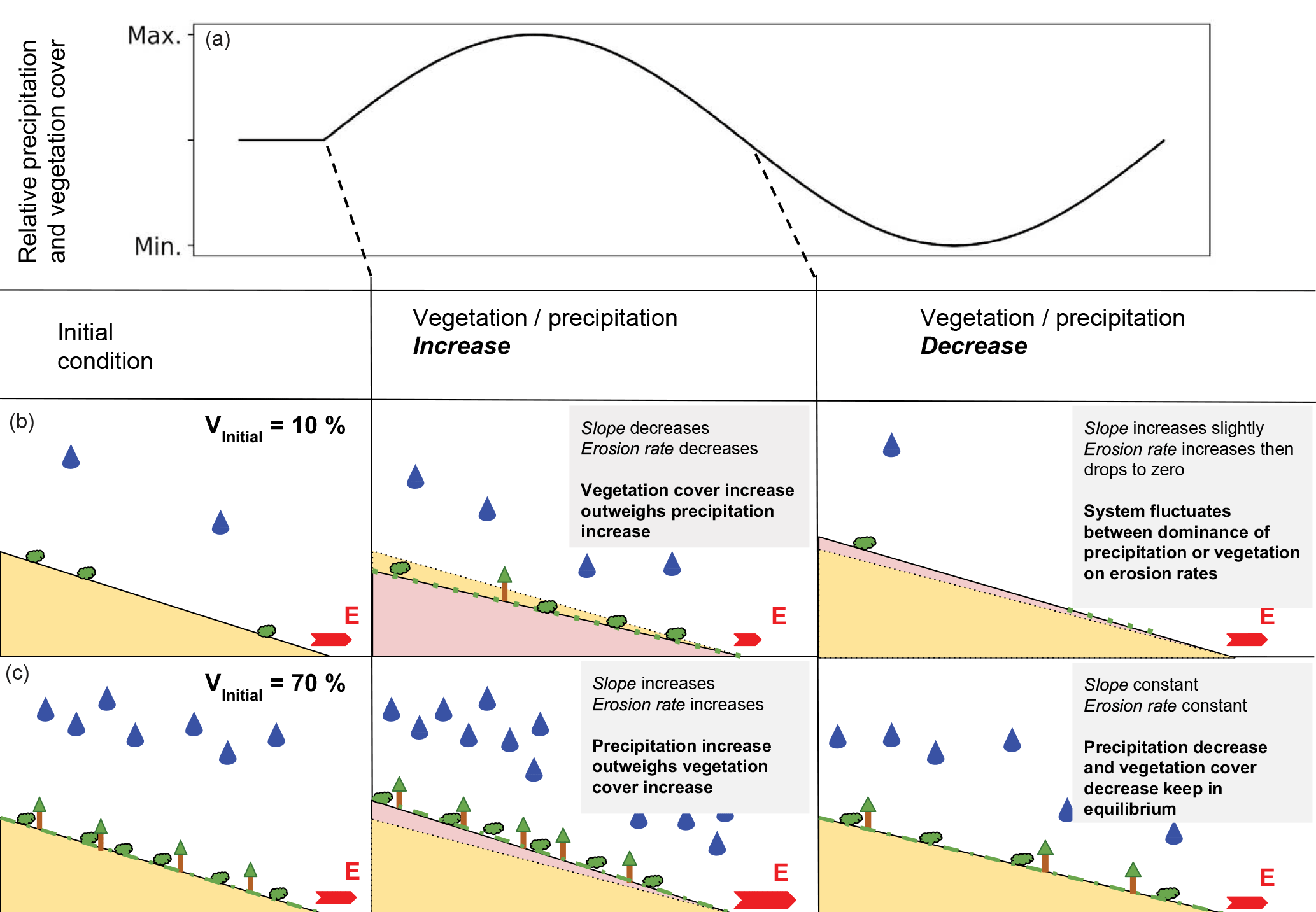
Figure 18 Conceptual figure showing the topographic response from simulations with coupled oscillation of mean annual precipitation and vegetation cover (see Fig. 17 for erosion rates). Panel (a) illustrates transient forcings, panels (b) and (c) show the initial topography (yellow) and the resulting transient topography (pink). Changes in topography are not to scale. Vegetation and rainfall amounts are shown qualitatively on the hillslopes.

Lastly, a clearly different erosion rate behavior occurs for settings with higher vegetation cover (e.g., P(V=70 %), Fig. 17) compared to the previous lower vegetation cover scenarios. As the vegetation cover and precipitation increase (Fig. 17a) in the first half of the 100 kyr cycle, the erosion rates increase (to 0.35 mm yr⁻¹). This is due to the increase in precipitation, which outcompetes the decline in vegetation influenced erosivity/diffusivity parameters, K_d and K_v. Following this, when vegetation cover and precipitation decrease in the second half of the cycle, little to no change occurs in the erosion rates. This near static behavior in erosion rates while precipitation and vegetation cover decrease is due to an equilibrium between the negative effect on erosion rates for decreasing precipitation and the positive effect on erosion rates for decreasing vegetation cover.

In summary, the nonlinear shape of the vegetation dependent erosivity (K_v) and hillslope diffusivity (K_d) in combination with the linear effects of mean annual precipitation on erosion rates, exert a primary control on the direction and magnitude of change in catchment average erosion rates. Despite the simple oscillating behavior in precipitation and vegetation cover, a complex and nonlinear response in erosion rates occurs. In Fig. 18 we depicted the conceptual end-members of landscape behavior for the different scenarios of increasing or decreasing vegetation cover and mean annual precipitation for different initial landscapes. The implications of this are large for observational studies of catchment average erosion rates and suggest that the direction and magnitude of the response observed in a setting is highly dependent on the mean vegetation and precipitation conditions of the catchment, as well as when the observations are made within the cycle of varying vegetation and precipitation. Furthermore, these results highlight the need for future modeling studies (and motivation for our ongoing work) to investigate the response of catchment topography and erosion rates to more realistic climate and vegetation change scenarios. A broader range of initial vegetation covers and precipitation rates than those explored here would also be beneficial, such that the threshold in behavior between the two curves shown in Fig. 17b can be understood.

5.5 Potential observational approaches to test model predictions

The behavior discussed in the previous section matches field data reported by Owen et al. (2010) who analyzed soil production rates from bedrock in different climate regimes. This data, under the assumption of steady-state soil thickness, can be translated into denudation rates. The data show that for low values of mean annual precipitation, soil production rates vary between 0 and 2 m Ma⁻¹ due to the abiotic processes controlling soil production rates. These observations resemble the effect of our simulations with a 10 % initial vegetation cover, which shows the same variations in erosion rates with intervals of a zero erosion rate for hyper-arid conditions (Fig. 17). Areas with higher values of mean annual precipitation show higher values for the soil production rate. These data points were not corrected for different uplift rates in the sample areas, so it is not possible to isolate the effect of vegetation/precipitation and tectonic uplift. In general, the observations show no clear isolated trend but more of a cluster of soil production rates among a common mean, situated in a zone controlled by biotic conditions. Compared to our model data for simulations with 70 % initial vegetation cover, this resembles the nonintuitive behavior of an increase in erosion rate for increasing values of vegetation cover and precipitation compared to a constant erosion rate for decreasing values of vegetation cover and precipitation.

Schaller et al. (2018) and Oeser et al. (2018) present millennial timescale (cosmogenic radionuclide derived) hillslope denudation, and soil production, rates from the Chilean (EarthShape) study areas (Fig. 1a) considered in this paper. They find the lowest hillslope denudation rates in the arid and poorly vegetated north. Moving south towards higher precipitation and vegetation cover the denudation rates increase until the southernmost location, with highest rainfall and vegetation cover, where denudation rates decrease again. This nonlinear relationship of hillslope denudation rates with vegetation cover and precipitation is not directly comparable to the results presented here, but is consistent with (a) the notion emphasized here that interactions between precipitation and vegetation cover on denudation are nonlinear, and (b) that the study areas considered here, although tectonically quiescent for tens of millions of years, have varying denudation rates that suggest either variable rock uplift rates, and/or a persistent state of transience in hillslope denudation induced by millennial timescale oscillations in climate and vegetation.

Beyond the previous studies, limited observations are available for comparison to the predictions shown here. The millennial to million-year timescales investigated here can best be evaluated from observations of catchment-wide denudation over similar timescales. Cosmogenic radionuclide measurements from modern river sediments offer one means to evaluate these results. Work by Acosta et al. (2015) in east Africa and Olen et al. (2016) in the Himalayas, are also consistent with the results presented here for the range of vegetation cover available in each of these areas. However, the integration timescales that these studies are sensitive to are shorter than what is presented here and prohibit a detailed comparison. A final approach that future studies could pursue is to calculate paleo-denudation rates for catchments from a time series of sediment deposits preserved in either lakes (e.g., Marshall et al., 2015) or fluvial river terraces (e.g., Schaller and Ehlers, 2006; Schaller et al., 2016). However, to be most effective, these studies need to target multiple study areas with terrace or lake deposits that span a range of vegetation covers in the upstream catchments.

5.6 Model restrictions and caveats

Similar to previous work on this topic (Collins et al., 2004; Istanbulluoglu and Bras, 2005), the model setup used in this study was simplified to document how different vegetation and climate related factors impact topography over long (geologically relevant) timescales. We acknowledge that future model studies should address some of the restrictions imposed by our approach to evaluate their significance for the results presented here. Future work should consider a transport-limited fluvial model or a fully coupled alluvial sedimentation and transport model. These additions could bring new understanding regarding how vegetation not only influences detachment limited systems, but also influences sedimentation and entrainment of material. However, this added level of complexity could limit (due to computational concerns) the temporal scales over which an investigation like this could be conducted. Future studies could improve upon this work by considering a more in-depth parameterization of how vegetation related processes (e.g., changes in root depth and density, plant functional type) influence topographic metrics and erosion rates. Also, although supported by various publications (Dunne et al., 1995, 2010), the assumption of a nonlinear response of the effectiveness of diffusional and fluvial processes to increases in vegetation cover has a major impact on the results of this study. A better field-based understanding of these processes, and the relationships involved, could improve the accuracy of model studies like this.

Furthermore, due to the long timescales considered here, mean annual precipitation rather than a stochastic distribution of precipitation was implemented. Future work should evaluate how stochastic distributions in precipitation and extreme events in arid, poorly vegetated settings, impact these results. However, the long timescale forcings in precipitation and vegetation imposed in this study will likely persist as the background template upon which high-frequency changes are active.

Regarding the vegetation and water budget, a more sophisticated model of evapotranspiration and infiltration as a function of surface plant cover and plant functional traits, such as rooting depth, would improve model predictions and is a priority for our future work. Improvements will come from the planned coupling of the surface process model with the dynamic vegetation model LPJ-GUESS (Werner et al., 2018; Smith et al., 2014).

Our assumption that an increase in surface vegetation cover directly translates to an increase in Manning roughness is an additional simplification. The real value of the Manning roughness of a surface will be a function of the fractional densities of different plant communities per model patch. However, we argue that this simplification is necessary because it is not possible to know the composition of the plant community for specific areas at our modeled timescales. This could be resolved by fully coupling a landscape evolution model to a dynamic vegetation model to resolve inter-patch differences of surface vegetation cover and intra-patch plant functional types.

We also acknowledge that the transient forcings we have chosen for driving our model are simplistic and could be improved by a higher-fidelity time series of climate over the last millennia. We choose a 100 kyr, eccentricity driven, periodicity because it is widely recognized that the eccentricity cycles have been a main control driving Earth's glacial cycle over the last 0.9 Ma. While this approach is reasonable for a sensitivity analysis such as the one we have conducted, it prohibits a detailed comparison to observations in specific study areas without additional refinement. Our results suggest that a shorter periodicity, which would resemble other periodicities in the Milankovitch cycle (e.g., 41, 23 kyr) or shorter timescale climate variations such as Heinrich events (see Huntley et al., 2013), would lead to smaller magnitudes of adjustment to new dynamic equilibria, because of short time spans in highly erosive or only slightly erosive climate conditions within one period. Regarding the long time-periods considered, we chose to have a steady-state climate driver in the model without frequency driven modulation of rainfall events. We argue that over large timescales the occurrence of these events can be integrated into a meaningful mean value but acknowledge that the incorporation of those events could alter the results on a short cycle basis. However, because there is no meaningful way to test these frequency distributions against past climates, this would add additional unknowns and assumptions into our model parameterization.

Finally, we emphasize that a subset of our results, which resemble small magnitude changes of topographic relief (e.g., factor of change 1.01, Sect. 4.3.1, 4.3.2), are valid results for the predicted synthetic landscapes in our model framework and not a numerical artefact. However, we acknowledge that these predicted changes are too small to be measured in a real-world setting.

6 Conclusions

The results from our experiments show that the interaction of vegetation cover and mean annual precipitation on the evolution of landscapes is a complex system with competing effects. The main conclusions that emerge from this study are as follows:

• i.

  Vegetation cover has a hindering effect on hillslope and fluvial erosion, but the magnitude at which changes in vegetation cover affect these processes is a function of the initial state of the system. Changes in systems with higher initial values of vegetation cover have a less pronounced effect than changes in systems with lower initial vegetation cover.

• ii.

  The relationship between precipitation and surface vegetation cover in the Chilean Coastal Cordilleras, shows a distinct shape: for a 10 % increase in surface vegetation cover, the corresponding increase in the mean annual precipitation is smaller in areas of lower vegetation cover and increases for areas with higher vegetation cover. This has an effect on transient topographies by shifting the equilibrium of vegetation and precipitation effects on erosion rates.

• iii.

  Following our step-change simulations, model results show different behaviors for changes in vegetation cover and mean annual precipitation. While increases in mean annual precipitation have an increasing effect on erosion rates and a related long-term negative effect on topographic metrics, an increase in vegetation cover hinders erosion and leads to higher topographic metrics. The magnitude of these changes is again dependent on the initial vegetation cover and precipitation before the step change.

• iv.

  Simulations with either oscillating vegetation cover or oscillating precipitation show adjustments to new dynamic mean values around which the basin metrics oscillate. The magnitude of the adjustment is highly sensitive to initial vegetation cover, where simulations with 10 % initial cover show higher magnitudes than simulations with 70 % cover, for oscillating vegetation. Oscillating precipitation leads to lower/no adjustments and an oscillation of basin metrics around the initial mean values with generally lower amplitudes compared to simulations with oscillating vegetation cover.

• v.

  Simulations with coupled oscillations of both vegetation cover and precipitation show only small magnitudes of adjustments in topography metrics to new dynamic equilibrium, similar to simulations with a oscillation in only precipitation. However, corresponding erosion rates show a complex pattern of rapid increases and decreases, which results from an interplay of competing effects such as the hindering of erosion by vegetation and the aiding of erosion by precipitation.

Interpreted together, the above findings from this study highlight a highly variable behavior regarding how variations in vegetation cover impact erosion and topographic properties. The complexity of how vegetation cover and precipitation changes influence topography demonstrates the need for future work to consider both of these factors in tandem, rather than singling either parameter out (vegetation cover or precipitation), in order to understand potential transients in topography.