the Creative Commons Attribution 4.0 License.
the Creative Commons Attribution 4.0 License.
 | 17 Oct 2018
Short communication: Increasing vertical attenuation length of cosmogenic nuclide production on steep slopes negates topographic shielding corrections for catchment erosion rates
Interpreting catchment-mean erosion rates from in situ produced cosmogenic 10Be concentrations in stream sediments requires calculating the catchment-mean 10Be surface production rate and effective mass attenuation length, both of which can vary locally due to topographic shielding and slope effects. The most common method for calculating topographic shielding accounts only for the reduction of nuclide production rates due to shielding at the surface, leading to catchment-mean corrections of up to 20 % in steep landscapes, and makes the simplifying assumption that the effective mass attenuation length for a given nuclide production mechanism is spatially uniform. Here I evaluate the validity of this assumption using a simplified catchment geometry with mean slopes ranging from 0 to 80∘ to calculate the spatial variation in surface skyline shielding, effective mass attenuation length, and the total effective shielding factor, defined as the ratio of the shielded surface nuclide concentration to that of an unshielded horizontal surface. For flat catchments (i.e., uniform elevation of bounding ridgelines), the effect of increasing vertical attenuation length as a function of hillslope angle and skyline shielding exactly offsets the effect of decreasing surface production rate, indicating that no topographic shielding correction is needed when calculating catchment-mean vertical erosion rates. For dipping catchments (as characterized by a plane fit to the bounding ridgelines), the catchment-mean surface nuclide concentrations are also equal to that of an unshielded horizontal surface, except for cases of extremely steep range-front catchments, where the surface nuclide concentrations are counterintuitively higher than the unshielded case due to added production from oblique cosmic ray paths at depth. These results indicate that in most cases topographic shielding corrections are inappropriate for calculating catchment-mean erosion rates, and are only needed for steep catchments with nonuniform distributions of quartz and/or erosion rate. By only accounting for shielding of surface production, existing shielding approaches introduce a slope-dependent systematic error that could lead to spurious interpretations of relationships between topography and erosion rate.
- Article
(9247 KB) - Full-text XML
-
Supplement
(54 KB) - BibTeX
- EndNote


Measurement of in situ produced cosmogenic 10Be concentrations in stream sediments has rapidly become the primary tool for quantifying catchment-scale erosion rates over timescales of 103–105 years (Brown et al., 1995; Granger et al., 1996; von Blanckenburg, 2006; Portenga and Bierman, 2011; Codilean et al., 2018). Although requiring a number of simplifying assumptions about the steadiness of erosion and sediment transport (Bierman and Steig, 1996), erosion rates determined from 10Be concentrations in stream sediments have yielded insights into a number of key questions in tectonic geomorphology regarding the sensitivity of erosion rates to spatiotemporal patterns of climate, tectonics, and rock strength (e.g., Safran et al., 2005; Binnie et al., 2007; Ouimet et al., 2009; DiBiase et al., 2010; Bookhagen and Strecker, 2012; Miller et al., 2013; Scherler et al., 2017).
In contrast to point measurements, where a clear framework exists for converting 10Be concentrations to either a surface exposure age or steady erosion rate (e.g., Balco et al., 2008; Marrero et al., 2016), the interpretation of 10Be concentrations in stream sediment requires accounting for the spatial variation in elevation, latitude, quartz content, and erosion rate throughout a watershed (Bierman and Steig, 1996; Granger and Riebe, 2014). Additionally, topographic shielding corrections that account for the reduction of cosmic radiation flux on sloped or skyline-shielded point samples (Dunne et al., 1999) are applied to varying degrees for determining catchment-mean production rates. These shielding corrections are either applied at the pixel level (e.g., Codilean, 2006), catchment level (e.g., Binnie et al., 2006), or not at all (e.g., Portenga and Bierman, 2011). Although typically small (< 5 %), topographic corrections can be as large as 20 % for steep catchments (e.g., Norton and Vanacker, 2009). Because these corrections vary as a function of slope and relief, any systematic corrections can influence interpretations of relationships between topography and erosion rate.
The pixel-by-pixel skyline-shielding algorithm of Codilean (2006) results in the largest topographic shielding corrections, and has gained popularity due to its ease of implementation in the software packages TopoToolbox (Schwanghart and Scherler, 2014) and CAIRN (Mudd et al., 2016), the latter of which was used to recalculate published 10Be-derived catchment erosion rates globally as part of the OCTOPUS compilation project (Codilean et al., 2018). A key simplification of the Codilean (2006) approach is that it accounts only for the skyline shielding of surface production, and not for the change in shielding with depth, which determines the sensitivity of the effective mass attenuation length for nuclide production as a function of surface slope and skyline shielding (Dunne et al., 1999; Gosse and Phillips, 2001). Because a change in the effective mass attenuation length will directly influence the inferred erosion rate of a sample (Lal, 1991), the full depth-integrated implications of topographic shielding must be accounted for when inferring catchment erosion rates from 10Be concentrations in stream sediments.
Here I model the shielding of incoming cosmic radiation flux responsible for spallogenic production at both the surface and at depth for a simple catchment geometry to evaluate, as a function of catchment slope and relief, the total effect of topographic shielding on surface nuclide concentrations and the partitioning of shielding into surface skyline shielding and changes to the effective mass attenuation length. I then apply this framework to catchments that have a net dip (i.e., dipping plane fit to boundary ridgelines) and compare calculations of total shielding to those from typical pixel-by-pixel skyline-shielding corrections.
The incoming cosmic ray intensity, I(θ,d), responsible for in situ cosmogenic nuclide production by neutron spallation can be most simply described as a function of the incident ray path inclination angle above the horizon, θ, and the mass distance, d (g cm−2), traveled along that pathway:
where I0 is the maximum cosmic ray intensity at the surface, m is an exponent typically assumed to have a value of 2.3 (e.g., Nishiizumi et al., 1989), and λ is the mass attenuation length (g cm−2) for unidirectional incoming radiation (Dunne et al., 1999). The mass attenuation length for unidirectional radiation, λ, differs from the nominal mass attenuation length that describes cosmogenic nuclide production as a function of depth, Λ, due to the integration of radiation from all incident angles. Assuming m=2.3, a value of λ=1.3Λ results in a close match for horizontal unshielded surfaces with exponential production profiles typical of spallation reactions (Dunne et al., 1999; Gosse and Phillips, 2001).
For a horizontal surface sample (d=0), the unshielded total cosmic radiation flux, F0, is described by
where φ is the azimuthal angle of incoming radiation, and the term cosθ accounts for the convergence of the spherical coordinate system. For point samples that are either at depth (d>0) or have an incomplete view of the sky due to topographic shielding by thick (d≫λ) objects, the total cosmic radiation flux, F, is modulated by a shielding factor, S, such that
where θ0(φ) is the inclination angle above the horizon of topographic obstructions in the direction φ and d(θ,φ) varies as a function of both ray path azimuth and inclination angle (Dunne et al., 1999; Gosse and Phillips, 2001).
Equation (3) has two implications for interpreting exposure ages or erosion rates from cosmogenic nuclide concentrations of samples partially shielded by skyline topography (θ0(φ)>0). First, skyline shielding will reduce the surface production rate of cosmogenic nuclides by a factor of S0:
Second, due to shielding of low-intensity cosmic radiation below incident angles of θ0(φ), the effective mass attenuation length, Λeff, will increase relative to the nominal mass attenuation length for describing cosmogenic nuclide production as a function of depth, Λ (Dunne et al., 1999; Gosse and Phillips, 2001). For calculating surface exposure ages, only the reduction in surface production rate due to skyline shielding needs to be taken into account, and Eq. (4) is easily calculated for single points in the landscape (e.g., Balco et al., 2008). However, for determining erosion rates both the surface shielding and changing effective attenuation length must be accounted for, which requires solving Eq. (3) numerically as a function of vertical depth below the surface, as described in Sect. 3 below.
The importance of accounting for both changes in surface production rate, P, and changes in the effective mass attenuation length, Λeff, is illustrated by the analytical solution for nuclide concentration, C, measured on a steadily eroding surface for a stable nuclide with an exponential decrease in production rate with depth:
where E is erosion rate (g cm−2 yr−1; Lal, 1991). From Eq. (5) it is clear that increasing Λeff counters the effect of decreasing P in determining the surface nuclide concentration (or alternatively for inferring erosion rate).
For stream sediment samples that require calculating cosmogenic nuclide production rates across an entire catchment, solving Eq. (3) as a function of depth is presently too computationally intensive to be practical. Consequently, numerical implementations of topographic shielding calculations at the catchment scale make the simplifying assumption that Λeff=Λ, and thus S=S0 (Codilean, 2006; Schwanghart and Scherler, 2014; Mudd et al., 2016), accounting only for the effect of decreasing surface production rate, P. Here I use a simplified catchment geometry to solve Eq. (3) and directly calculate the impact of topographic shielding and surface slope on interpretations of catchment erosion rates from cosmogenic nuclide concentrations in stream sediments. For simplicity, I assume that cosmogenic nuclides are only produced by neutron spallation (i.e., Λ=160 g cm−2) and that the erosion rate is high enough that radioactive decay is negligible (i.e., E > 0.01 g cm−2 yr−1 for 10Be).
Throughout the analysis below, both the effective mass attenuation length, Λeff, and erosion rate, E, are defined in the vertical, rather than slope-normal direction. The vertical (with respect to the geoid) reference frame was chosen for three reasons. First, most studies report erosion rate as a vertical lowering rate and assume primarily vertical exhumation pathways. Second, treatment of slope-normal processes introduces a grid-scale dependence of erosion and shielding calculations that varies with topographic roughness (Norton and Vanacker, 2009). Third, for the case of uniform erosion rate, the resulting shielding calculations do not depend on the choice of reference frame, as long as the orientation of Λeff and E are defined similarly.
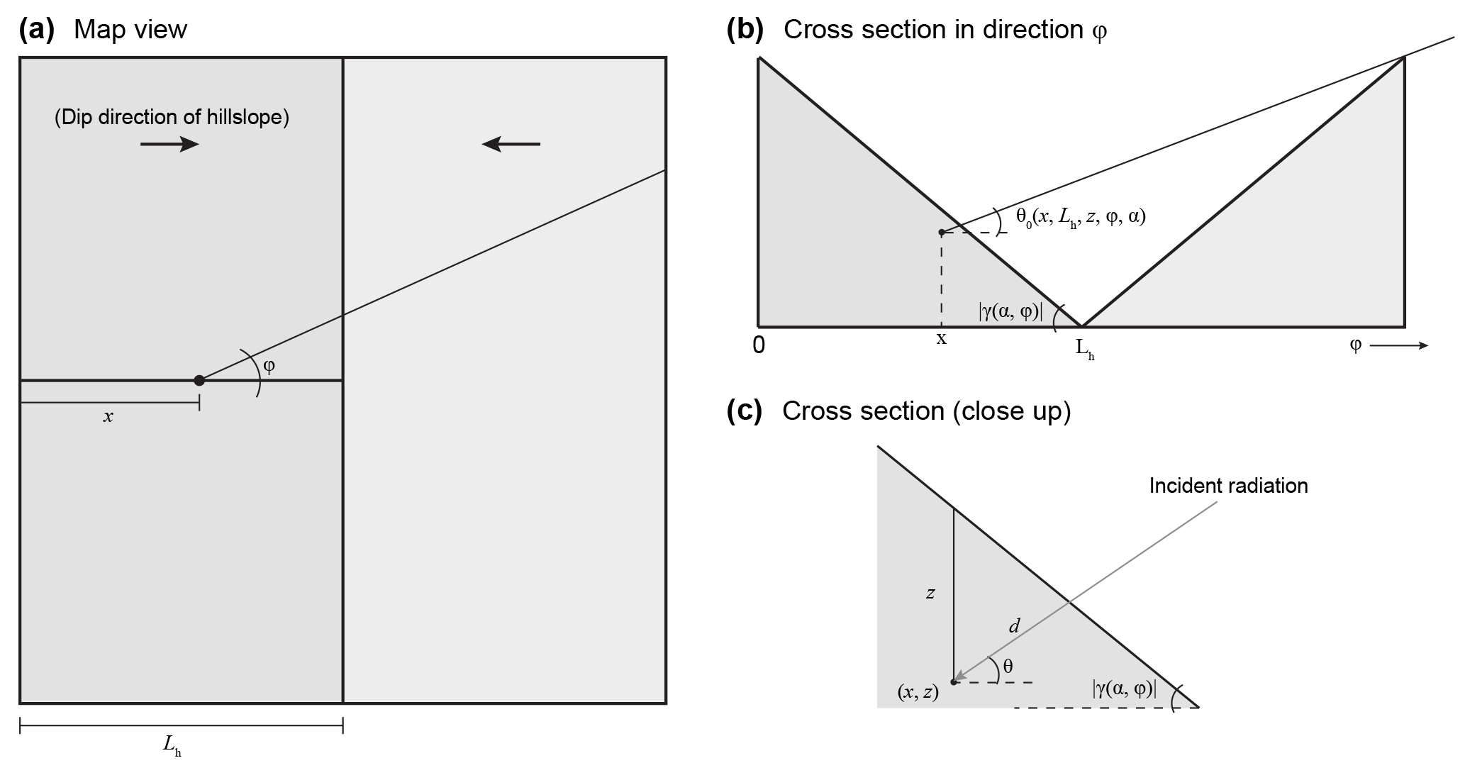
Figure 1Model catchment setup, showing (a) map view, (b) cross section along azimuthal angle φ (note that |γ|=α for φ=0), and (c) close-up of hillslope cross section.

Figure 2Dipping catchment shielding geometry, illustrated using example from the San Gabriel Mountains, California, USA. Image is centered on 34.20∘ N, 117.61∘ W. Colored lines indicate planes fit through bounding ridgelines dipping at angle β. indicates mean surface skyline-shielding parameter calculated using algorithm of Codilean (2006), and indicates the mean total effective shielding factor calculated from the simplified catchment geometry.
3.1 Simplified catchment geometry and model setup
Catchment geometry is simplified as an infinitely long v-shaped valley with width 2Lh and uniform hillslope angle α (Fig. 1). Because the ridgelines have uniform elevation, there is no net dip to the catchment; the effect of valley inclination will be assessed in Sect. 3.3. At a horizontal distance from the ridgeline x and vertical depth below the surface z, the shielding factor, S(x,z), is defined as
where ρ is rock density and γ is the apparent dip of the hillslope in the azimuthal direction φ (Fig. 1b). The inclination angle integration limit, θ0, is a function of topographic skyline-shielding inclination, and can be determined geometrically (Fig. 1) as
The apparent dip, γ, can be derived from the model geometry in Fig. 1 as
and the mass distance traveled through rock by a given incident ray as
Equation (5) was numerically solved for a series of hillslopes over a grid of with horizontal spacing and vertical spacing . To characterize mean slope controls on the shielding factor, S(x,z), the above calculation was applied to nine hillslopes with mean slope, α, ranging from 0 to 80∘ in 10∘ increments. Because for most natural landscapes, the resulting distribution of shielding factors is independent of hillslope scale.
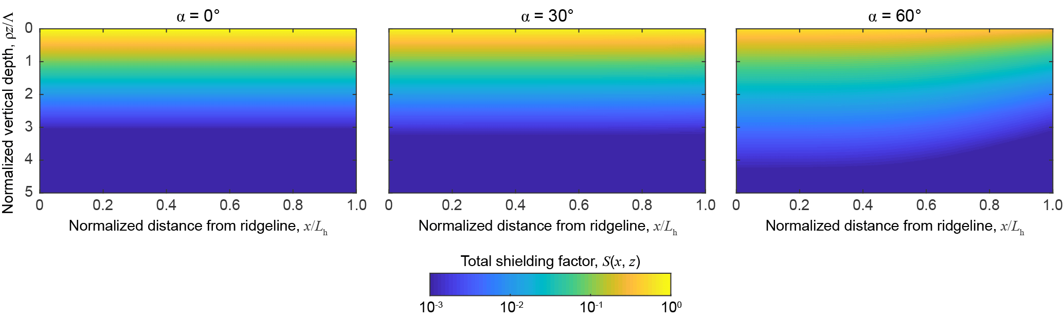
Figure 3Total shielding factor, S(x,z), as a function of normalized vertical depth and distance from ridgeline for varying hillslope angle, α.
3.2 Calculation of shielding parameters from model results
After applying Eq. (6) to a hillslope, it is straightforward to calculate the surface skyline-shielding component, . This skyline-shielding component should match the topographic shielding factor determined from the algorithm of Codilean (2006); for comparison this parameter was calculated at each pixel in the model catchment using TopoToolbox (Schwanghart and Scherler, 2014). Two additional parameters were calculated at each slope position using Eq. (5): the effective vertical mass attenuation length, Λeff(x), and the total effective shielding factor, Ceff(x).
Although spallogenic production of cosmogenic nuclides following Eq. (1) is well-described by an exponential decrease with depth for horizontal unshielded surfaces, this is not true in general for shielded samples (Dunne et al., 1999). The effective vertical mass attenuation length, Λeff(x), is approximated by the vertical depth below the surface at which the shielding factor is 5 % of the surface shielding (i.e., 3 e-folding lengths) such that
If nuclide production as a function of depth deviates from an exponential decline, it is inaccurate to use the analytical relationship between surface sample concentration, C(x) (atoms g−1), and steady-state vertical erosion rate, E (g cm−2 yr−1), typically applied to eroding samples
where P0(x) is the unshielded surface production rate, corrected for latitude and air pressure (Lal, 1991). Equation (11) derives from integrating the path history of a particle being exhumed vertically at a steady rate E and emerging at the surface with an accumulated nuclide concentration C(x):
which can be parameterized in terms of vertical depth below the surface, z, according to
where the depth of a rock parcel below the surface z0 at time t0 is deep enough such that there is no cosmogenic nuclide production ( for the calculations below) and is the time it takes for a rock parcel to travel from depth z0 to the surface (assuming a vertical exhumation pathway). Because there is no analytical solution for Eq. (13), the integral needs to be solved numerically. A total effective shielding factor, Ceff(x), acts as a correction factor to interpret local erosion rate from a sample concentration, defined by
where is the integrated shielding depth profile for the case α=0 (i.e., no slope or skyline shielding), and Ceff(x) does not depend on spatial variations in latitude or air pressure corrections. Finally, a mean effective shielding factor, , is defined for the whole hillslope as
which is equivalent to the catchment-mean shielding factor for the simplified valley geometry shown in Fig. 1.
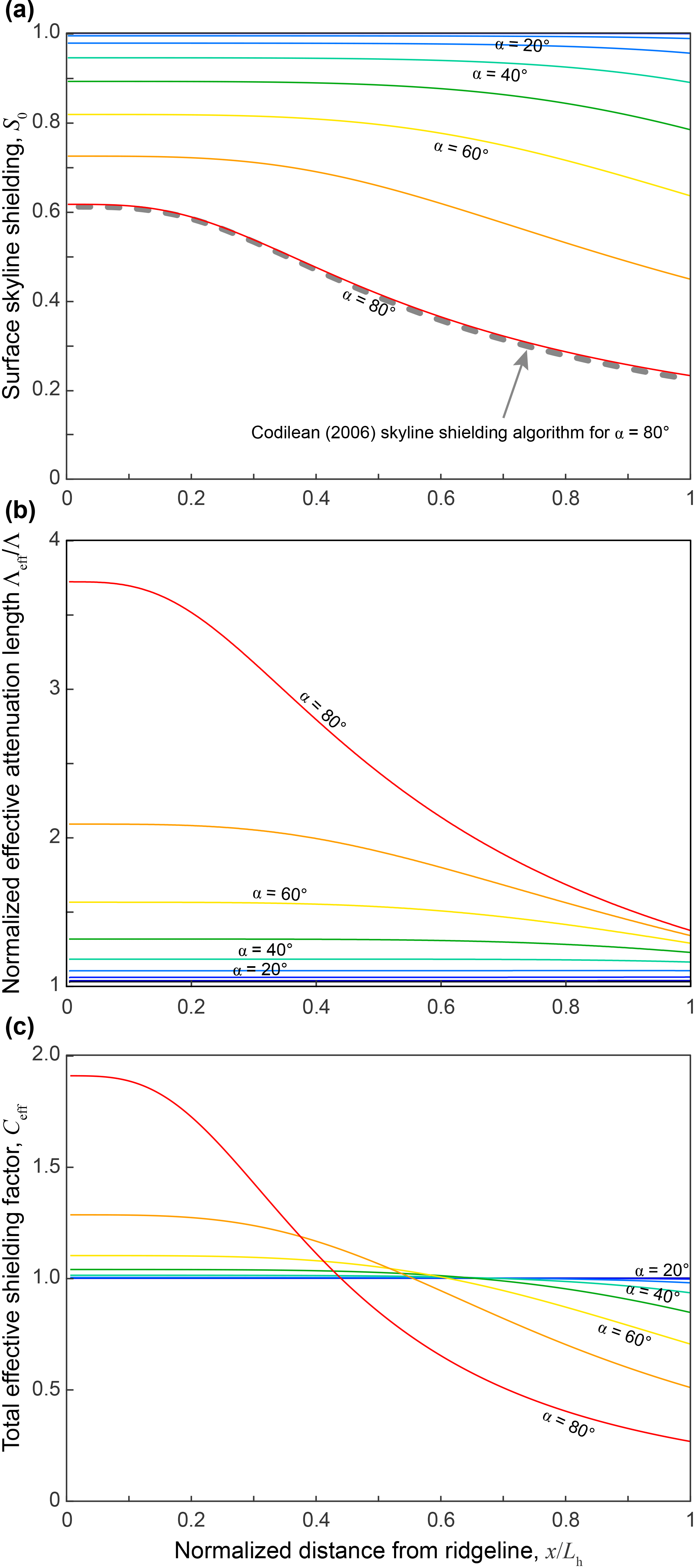
Figure 4Plots of (a) surface skyline-shielding factor (b) normalized effective vertical attenuation length, and (c) total effective shielding factor as a function of normalized distance from ridgeline for model runs with α=0–80∘. Dashed line in (a) indicates topographic shielding calculation using algorithm of Codilean (2006) applied to a digital elevation model of the case α=80∘.
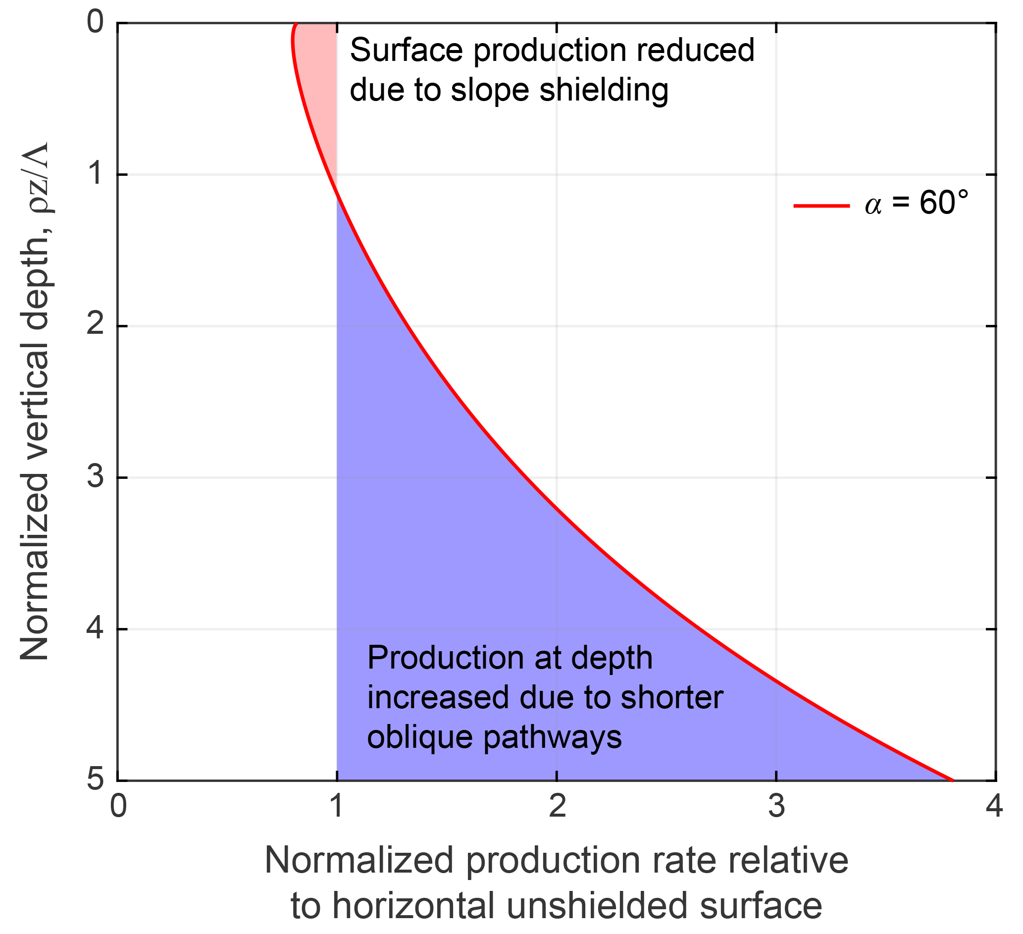
Figure 5Plot of normalized production rate relative to horizontal unshielded surface as a function of normalized vertical depth for a 60∘ slope with no additional skyline shielding. Near the surface, production rates are decreased due to slope shielding of incoming cosmic radiation; however, production rates at depth increase relative to the unshielded case due to additional radiation along shorter oblique pathways (Fig. 1c).
3.3 Approximation for dipping catchments
Although the above framework accounts for variations in catchment relief and hillslope angle, α, in all cases there is no net dip to the entire catchment (i.e., ridgeline elevations are uniform), which is not the case for natural watersheds. To simplify the geometry of a dipping catchment, I use a similar approach as Binnie et al. (2006) to model the catchment as a plane fit through the bounding ridgelines with dip β. I focus on two end-member cases, using examples from the San Gabriel Mountains, California, USA, for illustration (Fig. 2). First, for an “interior” catchment that is tributary to a larger valley within a mountain range, the catchment will have a net shielding similar to the geometry of the hillslope in Fig. 1. Consequently, the shielding geometry can be approximated by Eqs. (6)–(9) with α=β. For the case of an “exterior” catchment that has a net dip β but no opposing skyline shielding, Eq. (7) becomes
For both examples, I compared the catchment-mean shielding factor, , to the mean surface skyline-shielding factor, , as calculated using the commonly applied topographic shielding algorithm of Codilean (2006) in TopoToolbox (Schwanghart and Scherler, 2014).
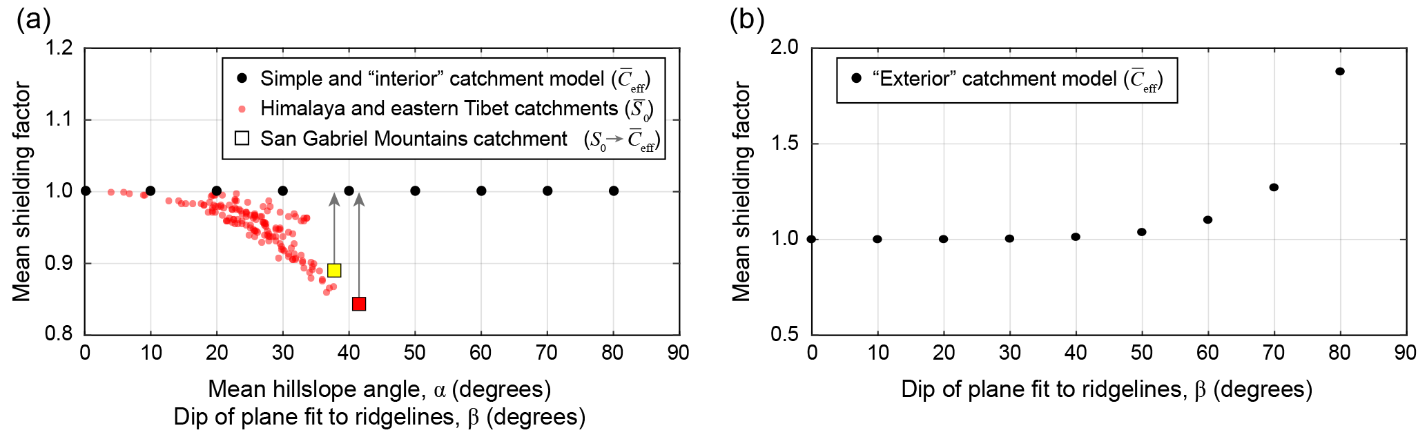
Figure 6Plots showing mean total shielding factor, , for (a) simple horizontal catchment case (Fig. 1) for varying mean hillslope angle, α, which is equivalent to the “interior” dipping catchment case as a function of catchment dip, β (Fig. 2), and (b), the mean total shielding factor, , for the “exterior” dipping catchment model as a function of catchment dip, β (Fig. 2). Red points in (a) indicate the relationship between the mean surface skyline-shielding factor, , as a function of mean hillslope angle for compilation of catchment 10Be data in the Himalaya and eastern Tibet as reported by Scherler et al. (2017). Red and yellow squares indicate the mean surface skyline factor, , calculated for example catchments from the San Gabriel Mountains (Fig. 2). Arrows indicate the difference between mean surface skyline-shielding factor and mean total shielding factor, .
For the catchment geometry shown in Fig. 1, the local shielding factor, S(x,z), decreases with increasing depth, z; distance downslope, x; and increasing slope, α (Fig. 3). The surface skyline-shielding factor, S0(x), decreases with distance downslope, x, and increasing hillslope angle, α, with the greatest shielding occurring in the valley bottoms of steep catchments (Fig. 4a). For the case α=80∘, comparison of S0(x) with the topographic shielding algorithm of Codilean (2006) shows that the two are equivalent (Fig. 4a).
The normalized effective attenuation length, Λeff∕Λ, decreases as a function of distance downslope and increases with increasing hillslope angle (Fig. 4b). Although cosmogenic nuclide production is concentrated at depths of for low slopes, production rates at depth for very steep slopes can be greater than those of flat landscapes, despite lower surface production rates (Fig. 5). This effect emerges in part due to the increased effective attenuation length for collimated radiation in skyline-shielded samples (up to a factor of 1.3 – Dunne et al., 1999; Gosse and Phillips, 2001), but mainly because on steep slopes a point at vertical depth z below the surface is receiving incident radiation from oblique pathways that can be shorter than those overhead (Fig. 1c). Consequently, there is an additional radiation flux that increases the effective vertical mass attenuation length, Λeff, an effect that is most pronounced near ridgelines ( where skyline shielding is minimized (Figs. 3, 4b).
The combined effect of the decrease in surface production (Fig. 4a) and the increase in effective attenuation length (Fig. 4b) leads to a pattern whereby the total effective shielding factor, Ceff(x), is greater than 1 along the upper portion of hillslopes and less than 1 along the lower portion of hillslopes near the valley bottom (Fig. 4c). Although there may be considerable variation in shielding depending on slope position for steep slopes (, the mean effective shielding parameter, , is unity for all cases (Fig. 6a).
For the case of dipping catchments (Fig. 2), the sensitivity of the mean effective shielding parameter to catchment dip, β, depends on whether catchments are “interior” (i.e., shielded by an opposing catchment) or “exterior” (i.e., no external skyline shielding). For “interior” catchments, the shielding calculations are identical to the analysis above, and thus is again unity for all cases (Fig. 6a). For “exterior” catchments, the increase in effective attenuation length at steep slopes due to shorter oblique radiation pathways (Fig. 1c) is larger than the decrease in surface production due to skyline shielding, and is greater than 1 (Fig. 6b). However, for all but the most extreme catchment dips (β≤40∘), is effectively 1 (within 1 %).
For the two example catchments in the San Gabriel Mountains (Fig. 2), the mean total effective shielding factor, , is 1.00, despite steep catchment dips (β=17 and 32∘) and high mean surface skyline shielding, ( and 0.84 as calculated by the algorithm of Codilean, 2006; Fig. 6a).
The above results indicate that no correction factor for topographic shielding is needed to infer catchment-mean erosion rates from 10Be concentrations in stream sediments for most cases, as long as the assumptions of spatially uniform quartz content and steady uniform erosion rate are valid. Only in the extreme case of an “exterior” catchment with mean dip β > 40∘ will such corrections be necessary. Although the approach of only calculating the surface skyline-shielding component of the total effective shielding factor is appropriate for calculating surface exposure ages, neglecting the slope and shielding controls on the effective mass attenuation length leads to a systematic underprediction of the actual erosion rate. The magnitude of this underprediction increases with increasing catchment mean slope, as highlighted by a compilation of catchment erosion rates from steep catchments in the Himalaya and eastern Tibetan Plateau (red data points, Fig. 5a).
For catchments with spatially variable quartz content or erosion rate, a spatially distributed total effective shielding factor, Ceff, must be calculated at each pixel. Although calculating the surface skyline-shielding component is straightforward (Codilean, 2006), solving Eq. (3) at depth for arbitrary catchment geometries is presently too computationally intensive to be practical. However, while not entirely transferable to arbitrarily rough topography (e.g., Norton and Vanacker, 2009), Fig. 4c suggests that for slopes less than 40∘, the total effective shielding factor does not vary significantly across the hillslope. For steep catchments with spatially variable quartz content or erosion rate, direct calculation of shielding at depth is likely needed to calculate the spatially distributed total effective shielding parameter. In particular, shielding calculations in landscapes dominated by cliff retreat are poorly suited for treatment in a vertical reference frame (e.g., Ward and Anderson, 2011).
The modeling approach above assumes a simplified angular distribution of cosmic radiation flux (Eq. 1) and only accounts for cosmogenic nuclide production via spallation. In actuality, the cosmic radiation flux does not go to zero at the horizon, and becomes increasingly collimated (higher m) with increasing atmospheric depth (Argento et al., 2015). Thus, the sensitivity of the effective mass attenuation length to shielding will increase with increasing elevation. However, the magnitude of changes in the effective mass attenuation length due to shielding-induced collimation is at most 30 % (Dunne et al., 1999), compared to the potential factor of 3 or more increase due to shorter oblique radiation pathways on very steep slopes (Figs. 1c; 4b). For hillslope gradients commonly observed in cosmogenic nuclide studies of steep landscapes (30–40∘), the increase in effective mass attenuation length due to shielding-induced collimation and slope effects are 2 %–5 % and 6 %–15 %, respectively (Dunne et al., 1999; Fig. 4b). The dependence of Λ on atmospheric depth, which is typically not accounted for in catchment erosion studies, is minor (< 10 % for extreme case of catchment with 4 km of relief Marrero et al., 2016) compared to the above slope effect for most landscapes. Treatment of cosmogenic nuclide production by muons is less constrained than spallogenic production, but the angular distribution of production by muons is likely similar to that for spallation reactions and also sensitive to latitude and atmospheric depth (Heisinger et al., 2002a, b).
Overall, the effect of topographic shielding corrections on interpreting catchment erosion rates is small compared to typical assumptions inherent to detrital cosmogenic nuclide methods. In particular, the assumption of steady lowering is likely to be increasingly inappropriate for rapidly eroding landscapes characterized by a significant contribution of muonogenic production or slowly eroding landscapes where 10Be concentrations integrate over glacial–interglacial climate cycles. Steep landscapes characterized by stochastic mass wasting present additional complications (Niemi et al., 2005; Yanites et al., 2009), requiring the nontrivial calculation of spatially distributed shielding parameters for an arbitrary catchment geometry. Nonetheless, in all cases accounting only for surface skyline shielding (e.g., Codilean, 2006) without including its concurrent influence on the effective attenuation length yields incorrect results.
The simplified model presented here for catchment-scale topographic shielding of incoming cosmic radiation highlights the two competing effects of slope and skyline shielding. As catchment relief increases, surface production rates are reduced due to increased skyline shielding. However, for shielded samples radiation is increasingly collimated, and for sloped surfaces oblique radiation pathways increase nuclide production at depth. Both of these effects lead to deeper effective vertical mass attenuation lengths, which offset the reduction in surface production when inferring erosion rates from cosmogenic nuclide concentrations. At the catchment scale, the mean total effective shielding factor is 1 for a large range of catchment geometries, suggesting that topographic shielding corrections for catchment samples are generally not needed, and that applying commonly used topographic shielding algorithms leads to underestimation of true erosion rates by up to 20 %. Although these corrections are typically small compared to other methodological uncertainties, they vary systematically with slope and relief. Consequently, misapplication of shielding correction factors could influence interpretations of relationships between topography and erosion rate.
MATLAB codes used to generate Figs. 3, 4, and 6 are included as Supplement and available at: https://github.com/romandibiase/catchment-shielding (last access: 15 October 2018).
The supplement related to this article is available online at: https://doi.org/10.5194/esurf-6-923-2018-supplement.
The author declares that there is no conflict of interest.
This project was supported by funding from National Science Foundation grant
EAR-160814, and benefited from discussions with Kelin Whipple, Alexander Neely, Paul Bierman.
Review comments from Greg Balco, Dirk Scherler, and an anonymous reviewer
helped improve the manuscript.
Edited by: Jane Willenbring
Reviewed by: Greg Balco and one anonymous referee
Argento, D. C., Stone, J. O., Reedy, R. C., and O'Brien, K.: Physics-based modeling of cosmogenic nuclides part II – Key aspects of in-situ cosmogenic nuclide production, Quat. Geochronol., 26, 44–55, https://doi.org/10.1016/j.quageo.2014.09.005, 2015.
Balco, G., Stone, J. O., Lifton, N. A., and Dunai, T. J.: A complete and easily accessible means of calculating surface exposure ages or erosion rates from 10Be and 26Al measurements, Quat. Geochronol., 3, 174–195, https://doi.org/10.1016/j.quageo.2007.12.001, 2008.
Bierman, P. and Steig, E. J.: Estimating rates of denudation using cosmogenic isotope abundances in sediment, Earth Surf. Proc. Land., 21, 125–139, https://doi.org/10.1002/(SICI)1096-9837(199602)21:2<125::AID-ESP511>3.0.CO;2-8, 1996.
Binnie, S. A., Phillips, W. M., Summerfield, M. A., and Fifield, K. L.: Sediment mixing and basin-wide cosmogenic nuclide analysis in rapidly eroding mountainous environments, Quat. Geochronol., 1, 4–14, https://doi.org/10.1016/j.quageo.2006.06.013, 2006.
Binnie, S. A., Phillips, W. M., Summerfield, M. A., and Fifield, K. L.: Tectonic uplift, threshold hillslopes, and denudation rates in a developing mountain range, Geology, 35, 743–746, https://doi.org/10.1130/G23641A.1, 2007.
Bookhagen, B. and Strecker, M. R.: Spatiotemporal trends in erosion rates across a pronounced rainfall gradient: Examples from the southern Central Andes, Earth Planet. Sc. Lett., 327–328, 97–110, https://doi.org/10.1016/j.epsl.2012.02.005, 2012.
Brown, E. T., Stallard, R. F., Larsen, M. C., Raisbeck, G. M., and Yiou, F.: Denudation rates determined from the accumulation of in situ-produced 10Be in the luquillo experimental forest, Puerto Rico, Earth Planet. Sc. Lett., 129, 193–202, https://doi.org/10.1016/0012-821X(94)00249-X, 1995.
Codilean, A. T.: Calculation of the cosmogenic nuclide production topographic shielding scaling factor for large areas using DEMs, Earth Surf. Proc. Land., 31, 785–794, https://doi.org/10.1002/esp.1336, 2006.
Codilean, A. T., Munack, H., Cohen, T. J., Saktura, W. M., Gray, A., and Mudd, S. M.: OCTOPUS: An Open Cosmogenic Isotope and Luminescence Database, Earth Syst. Sci. Data Discuss., https://doi.org/10.5194/essd-2018-32, in review, 2018.
DiBiase, R. A., Whipple, K. X., Heimsath, A. M., and Ouimet, W. B.: Landscape form and millennial erosion rates in the San Gabriel Mountains, CA, Earth Planet. Sc. Lett., 289, 134–144, https://doi.org/10.1016/j.epsl.2009.10.036, 2010.
Dunne, J., Elmore, D., and Muzikar, P.: Scaling factors for the rates of production of cosmogenic nuclides for geometric shielding and attenuation at depth on sloped surfaces, Geomorphology, 27, 3–11, https://doi.org/10.1016/S0169-555X(98)00086-5, 1999.
Gosse, J. C. and Phillips, F. M.: Terrestrial in situ cosmogenic nuclides: theory and application, Quaternary Sci. Rev., 20, 1475–1560, https://doi.org/10.1016/S0277-3791(00)00171-2, 2001.
Granger, D. E. and Riebe, C. S.: Cosmogenic Nuclides in Weathering and Erosion, in Treatise on Geochemistry, Second Edition, edited by: Holland, H. D. and Turekian, K. K., Elsevier, Oxford 401–435, https://doi.org/10.1016/B978-0-08-095975-7.00514-3, 2014.
Granger, D. E., Kirchner, J. W., and Finkel, R.: Spatially Averaged Long-Term Erosion Rates Measured from in Situ-Produced Cosmogenic Nuclides in Alluvial Sediment, J. Geol., 104, 249–257, https://doi.org/10.1086/629823, 1996.
Heisinger, B., Lal, D., Jull, A. J. T., Kubik, P., Ivy-Ochs, S., Neumaier, S., Knie, K., Lazarev, V., and Nolte, E.: Production of selected cosmogenic radionuclides by muons: 1. Fast muons, Earth Planet. Sc. Lett., 200, 345–355, https://doi.org/10.1016/S0012-821X(02)00640-4, 2002a.
Heisinger, B., Lal, D., Jull, A. J. T., Kubik, P., Ivy-Ochs, S., Knie, K., and Nolte, E.: Production of selected cosmogenic radionuclides by muons: 2. Capture of negative muons, Earth Planet. Sc. Lett., 200, 357–369, https://doi.org/10.1016/S0012-821X(02)00641-6, 2002b.
Lal, D.: Cosmic ray labeling of erosion surfaces: in situ nuclide production rates and erosion models, Earth Planet. Sc. Lett., 104, 424–439, https://doi.org/10.1016/0012-821X(91)90220-C, 1991.
Marrero, S. M., Phillips, F. M., Borchers, B., Lifton, N., Aumer, R., and Balco, G.: Cosmogenic nuclide systematics and the CRONUScalc program, Quat. Geochronol., 31, 160–187, https://doi.org/10.1016/j.quageo.2015.09.005, 2016.
Miller, S. R., Sak, P. B., Kirby, E., and Bierman, P. R.: Neogene rejuvenation of central Appalachian topography: Evidence for differential rock uplift from stream profiles and erosion rates, Earth Planet. Sc. Lett., 369–370, 1–12, https://doi.org/10.1016/j.epsl.2013.04.007, 2013.
Mudd, S. M., Harel, M.-A., Hurst, M. D., Grieve, S. W. D., and Marrero, S. M.: The CAIRN method: automated, reproducible calculation of catchment-averaged denudation rates from cosmogenic nuclide concentrations, Earth Surf. Dynam., 4, 655–674, https://doi.org/10.5194/esurf-4-655-2016, 2016.
Niemi, N. A., Oskin, M., Burbank, D. W., Heimsath, A. M., and Gabet, E. J.: Effects of bedrock landslides on cosmogenically determined erosion rates, Earth Planet. Sc. Lett., 237, 480–498, https://doi.org/10.1016/j.epsl.2005.07.009, 2005.
Nishiizumi, K., Winterer, E., Kohl, C. P., Klein, J., Middleton, R., Lal, D., and Arnold, J. R.: Cosmic ray production rates of 10Be and 26Al in quartz from glacially polished rocks, J. Geophys. Res.-Solid, 94, 17907–17915, https://doi.org/10.1029/JB094iB12p17907, 1989.
Norton, K. P. and Vanacker, V.: Effects of terrain smoothing on topographic shielding correction factors for cosmogenic nuclide-derived estimates of basin-averaged denudation rates, Earth Surf. Proc. Land., 34, 145–154, https://doi.org/10.1002/esp.1700, 2009.
Ouimet, W. B., Whipple, K. X., and Granger, D. E.: Beyond threshold hillslopes: Channel adjustment to base-level fall in tectonically active mountain ranges, Geology, 37, 579–582, https://doi.org/10.1130/G30013A.1, 2009.
Portenga, E. W. and Bierman, P. R.: Understanding Earth's eroding surface with 10Be, GSA today, 21, 4–10, https://doi.org/10.1130/G111A.1, 2011.
Safran, E. B., Bierman, P. R., Aalto, R., Dunne, T., Whipple, K. X., and Caffee, M.: Erosion rates driven by channel network incision in the Bolivian Andes, Earth Surf. Proc. Land., 30, 1007–1024, https://doi.org/10.1002/esp.1259, 2005.
Scherler, D., DiBiase, R. A., Fisher, G. B., and Avouac, J. P.: Testing monsoonal controls on bedrock river incision in the Himalaya and Eastern Tibet with a stochastic-threshold stream power model, J. Geophys. Res.-Earth, 122, 1389–1429, https://doi.org/10.1002/2016JF004011, 2017.
Schwanghart, W. and Scherler, D.: Short Communication: TopoToolbox 2 – MATLAB-based software for topographic analysis and modeling in Earth surface sciences, Earth Surf. Dynam., 2, 1–7, https://doi.org/10.5194/esurf-2-1-2014, 2014.
von Blanckenburg, F.: The control mechanisms of erosion and weathering at basin scale from cosmogenic nuclides in river sediment, Earth Planet. Sc. Lett., 242, 224–239, https://doi.org/10.1016/j.epsl.2005.11.017, 2006.
Ward, D. and Anderson, R. S.: The use of ablation-dominated medial moraines as samplers for 10Be-derived erosion rates of glacier valley walls, Kichatna Mountains, AK, Earth Surf. Proc. Land., 36, 495–512, https://doi.org/10.1002/esp.2068, 2011.
Yanites, B. J., Tucker, G. E., and Anderson, R. S.: Numerical and analytical models of cosmogenic radionuclide dynamics in landslide-dominated drainage basins, J. Geophys. Res.-Earth, 114, F01007, https://doi.org/10.1029/2008JF001088, 2009.