Estimating the disequilibrium in denudation rates due to divide migration at the scale of river basins

Basin-averaged denudation rates may locally exhibit a wide dispersion, even in areas where the topographic steady state is supposedly achieved regionally. This dispersion is often attributed to the accuracy of the data or to some degree of natural variability of local erosion rates which can be related to stochastic processes such as landsliding. Another physical explanation of this dispersion is local and transient disequilibrium between tectonic forcing and erosion at the scale of catchments. Recent studies have shown that basin divide migration can potentially induce such perturbations, and they propose metrics to assess divide mobility based on cross-divide contrasts in headwater topographic features. Here, we use a set of landscape evolution models assuming spatially uniform uplift, rock strength and rainfall to assess the effect of divide mobility on basin-wide denudation rates. We propose using basin-averaged aggressivity metrics based on cross-divide contrasts (1) in channel χ, an integral function of position in the channel network; (2) in channel local gradient; and (3) in channel height, measured at a reference drainage area. From our simulations, we show that the metric based on differences in χ is the most reliable to diagnose local disequilibrium. The other metrics are more suitable for relatively active tectonic regions such as mountain belts, where contrasts in local gradient and elevation are more important. We find that the ratio of basin denudation associated with drainage migration to uplift can reach a factor of 2, regardless of the imposed uplift rate, erodibility, diffusivity coefficient or critical hillslope gradient. A comparison with field observations in the Great Smoky Mountains (southern Appalachians, USA) underlines the difficulty of using the metric based on χ, which depends on the – poorly constrained – elevation of the outlet of the investigated catchment. Regardless of the considered metrics, we show that observed dispersion is controlled by catchment size: a smaller basin may be more sensitive to divide migration and hence to disequilibrium. Our results thus highlight the relevance of divide stability analysis from digital elevation models as a fundamental preliminary step for basin-wide denudation rate studies based on cosmogenic radionuclide concentrations.

1 Introduction

Topographic steady state, in which average topography is constant over time, is one of the key concepts of modern geomorphology (e.g. Gilbert, 1877; Hack, 1960; Montgomery, 2001). Though simple, this paradigm provides a useful framework to study landscape evolution related to tectonic and/or climatic forcing (e.g. Willett et al., 2001; Reinhart and Ellis, 2015), to spatial variations in rock strength (Perne et al., 2017) or to the geometry of active crustal structures (Lavé and Avouac, 2001; Stolar et al., 2007; Scherler et al., 2014; Le Roux-Mallouf et al., 2015). To define topographic steady state, the temporal and spatial scales of the processes involved are essential parameters. Compared to large-scale geodynamic processes operating over 1–100 Myr timescales, river incision and sediment transport are rapid processes driving landscapes to stable forms over this long timescale, whereas rapid climatic fluctuations during the Quaternary may prevent the occurrence of steady-state conditions in modern landscapes (Whipple, 2001).

The timescale of divide migration has received increasing attention in recent years. Although rivers exhibit a rapid adjustment to tectonic or climatic changes to maintain their profiles, Whipple et al. (2017) show that divides continue to migrate over time periods of 10⁶–10⁷ years as a response to the same changes. This suggests that long-term transience might be pervasive in the planar structure of landscapes, even in the absence of new variations in landscape characteristics or forcings (e.g. tectonic or climate) (Hasbargen and Paola, 2000, 2003; Pelletier, 2004; Dahlquist et al., 2018). In addition to the influence of spatial variability of rock uplift rate, rock strength or rainfall (e.g. Reiners et al., 2003; Godard et al., 2006; Miller et al., 2013), this long timescale could also explain the persistence of spatial variations in denudation rates observed in tectonically inactive orogens which achieved regional-scale topographic steady state (Willett et al., 2014).

As an example, in the Great Smoky Mountains in the southern Appalachians, uplift and erosion rates integrated over varying time periods from 10 kyr to 100 Myr give a similar average magnitude of ca. 0.03 mm yr⁻¹ (Matmon et al., 2003a, b; Portenga and Bierman, 2011). These results suggest a regional quasi-topographic steady state over the last ∼180 Myr, maintained by the isostatic response of the thickened crust since the end of the Appalachian orogeny (Matmon et al., 2003a, b). Beyond this average value, individual basin-wide denudation rates exhibit a strong dispersion (up to a factor of 2, Fig. 1), which is not related to spatial variation in rainfall or in erodibility of the substrate (Matmon et al., 2003b). In a recent study, Willett et al. (2014) assess divide mobility from the contrast in the channel head topographic metric χ, taken here as a proxy for steady-state river profile elevation (Perron and Royden, 2012; Royden and Perron, 2013), and propose an explanation in which a significant part of the observed dispersion in denudation rates could be due to drainage divide migration associated with contrasting erosion rates across divides.

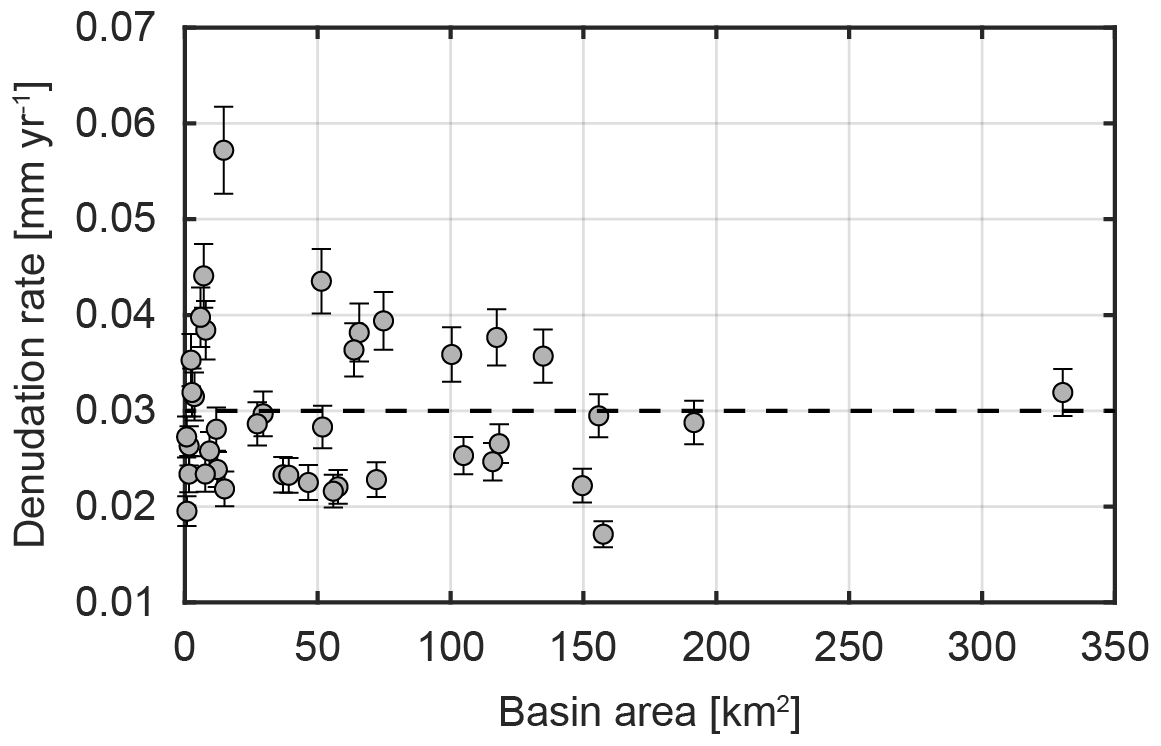
Figure 1 Basin-wide denudation rate variability as a function of drainage area in the Great Smoky Mountains. Original dataset from Matmon et al. (2003a, b); denudation rates reprocessed by Portenga and Bierman (2011). Dashed black line shows the estimated background uplift rate for the region of 0.03 mm yr⁻¹.

More recently, to characterize divide migrations, Forte and Whipple (2018) introduced other metrics, referred to as “Gilbert metrics” (Gilbert, 1877), based on the cross-divide contrast in channel local gradient and height. This last study indeed focused on cross-divide contrasts in headwater basin shape. Here, we propose extending these approaches by modelling divide migration and by developing new metrics to assess divide stability at the scale of the entire watershed, which are an expansion of the aggressivity metric initially suggested by Willett et al. (2014). We use these metrics to assess the effect of persistent divide mobility on basin-averaged erosion rates at a timescale of 10⁴ years. We use numerical landscape evolution models, taking into account both hillslope diffusion and fluvial incision. For the sake of simplicity and to avoid the influence of other factors such as topography, lithology, climate or vegetation, we restrict our analysis to synthetic orogens with spatially uniform uplift, rock strength and rainfall. After a brief presentation of our landscape evolution model (LEM), we describe the methods developed to assess basin-wide denudation rates and aggressivity metrics, such as average cross-divide contrasts in channel χ, gradient and height. Next, we investigate transient time and location of morphologic adjustments to divide migrations. We explore the relevance and complementarity of tested relative stability metrics between neighbouring basins. We then investigate the impact of uplift rate, erodibility and hillslope processes on the dynamics of divide migration and associated denudation rates. Finally, we apply our approach to the basin-wide denudation rates dataset of Matmon (2003a, b) in the case of the Great Smoky Mountains and propose new criteria to guide future sampling strategies to assess basin-wide denudation rates from river sands.

2 Methods

2.1 Landscape evolution model (LEM)

We use TTLEM (TopoToolbox Landscape Evolution Model) (Campforts et al., 2017), a landscape evolution model based on the MATLAB function library TopoToolbox 2 (Schwanghart and Scherler, 2014). This LEM uses a finite volume method (Campforts and Govers, 2015) to solve the following equation of mass conservation for rock or regolith subject to uplift and denudation:

$$\begin{array}{}\text{(1)}& {\displaystyle \frac{\partial z}{\partial t}}={\left({\displaystyle \frac{\partial z}{\partial t}}\right)}_{\mathrm{td}}+{\displaystyle \frac{{\mathit{\rho }}_{\mathrm{r}}}{{\mathit{\rho }}_{\mathrm{s}}}}U+{\left({\displaystyle \frac{\partial z}{\partial t}}\right)}_{\mathrm{hill}}+{\left({\displaystyle \frac{\partial z}{\partial t}}\right)}_{\mathrm{fluv}},\end{array}$$

where $\partial z/\partial t$ is the variation in elevation with time, $(\partial z/\partial t{)}_{\mathrm{td}}$ is the change of elevation due to tectonic horizontal advection, U is the rock uplift rate, and ρ_r∕ρ_s is the density ratio between the bedrock and the regolith. We use a linear formulation of hillslope diffusion (Culling, 1963) limited by a critical slope S_c:

$$\begin{array}{}\text{(2)}& {\left({\displaystyle \frac{\partial z}{\partial t}}\right)}_{\mathrm{hill}}=-\mathrm{\nabla }{q}_{\mathrm{s}}\mathrm{with}{q}_{\mathrm{s}}=-D\mathrm{\nabla }z,\end{array}$$

where q_s is the flux of soil or regolith material. When slope values exceed S_c, they are readjusted to the critical value by using a modified version of the excess topography algorithm (Blöthe et al., 2015). The diffusivity D gives the rate of soil or regolith material creep. Its magnitude ranges from 10⁻³ to 10⁻¹ m² yr⁻¹ in natural settings and varies with soil thickness, lithology and vegetation (Roering et al., 1999; Jungers et al., 2009; West et al., 2013; Richardson et al., 2019). Hillslope diffusion is implemented in TTLEM using an implicit scheme, which is unconditionally stable at large time steps (Pelletier, 2008). A non-linear diffusion formulation (Perron, 2011) is also implemented in TTLEM. However, we favoured the use of a linear diffusion with a critical slope, which is more convenient for the time step used in our simulations (5000 years) and the set of parameters considered (see Sect. 2.2). Due to the relatively coarse spatial resolution of our models (90 m), any of these diffusion formulations generate negligible topographic differences on the direct vicinity of crest lines (Roering et al., 1999, Campforts et al., 2017) and do not affect our results (see Fig. S1 in the Supplement). Fluvial incision is calculated with a stream power law:

$$\begin{array}{}\text{(3)}& {\left({\displaystyle \frac{\partial z}{\partial t}}\right)}_{\mathrm{fluv}}=-K{A}^m{\left({\displaystyle \frac{\partial z}{\partial x_{\mathrm{\Gamma }}}}\right)}^n,\end{array}$$

where K is the erodibility coefficient reflecting climate, hydraulic roughness, sediment load and lithology. Its value ranges between 10⁻¹⁶ and 10⁰ m^(1−2 m) yr⁻¹ (Kirby and Whipple, 2001; Harel et al., 2016). A is the upstream area. x_Γ is the along-stream distance from the outlet of the river. m and n are two parameters that are usually reported as a m∕n ratio ranging between 0.35 and 0.8. The river incision law is implemented in TTLEM using an explicit scheme based on a higher-order flux-limiting finite volume method (FVM) that is total variation diminishing (TVD-FVM) (see Campforts and Govers, 2015, and Campforts et al., 2017, for further details). Its main advantage is to eliminate numerical diffusion, which is present in most other schemes solving differential equations of river incision. This last point has a significant impact on the accuracy of basin-wide simulated denudation rates, making TTLEM a well-suited LEM for the purpose of this study.

2.2 Modelling approach and assumptions

2.2.1 Geometry and meshing

Since the computation is performed using a discretized land surface, smaller mesh sizes lead to detailed topography but lengthen the computation time and memory requirements. Hereinafter, we consider a reference square landscape model of 50 km side with a grid resolution of 90 m, which is a good compromise between computation time (3–5 h on a PC workstation) and the total amount of basins that can be studied (>1000). Our results are not affected when the grid resolution is 30 m nor when the model size is 100 km×100 km (see Fig. S2).

2.2.2 Boundary conditions

In order to isolate the effect of divide migrations on the variability of basin-wide denudation rates, we explore simple models with constant and spatially uniform uplift and precipitation rates, and we assume no horizontal advection, $(\partial z/\partial t{)}_{\mathrm{td}}=\mathrm{0}$. We use a Dirichlet boundary condition: simulation edges are not affected by uplift on a one pixel band to represent a stable base level for rivers. The model presents no initial topography, except for gaussian noise ranging between 0 and 50 m so as to initiate a random fluvial network.

2.2.3 Set of parameters

Firstly, we consider a reference model with parameters commonly used for moderately active orogens: an uplift rate U of 0.1 mm yr⁻¹, a diffusivity D of 10⁻² m² yr⁻¹ (Roering et al., 1999), a threshold slope S_c of 30^∘ (Burbank et al., 1996; Montgomery and Brandon, 2002; Binnie et al., 2007), and a m∕n ratio of 0.5 with m=0.5 and n=1, an erodibility coefficient K of $\mathrm{1}\times {\mathrm{10}}^{-\mathrm{5}}$ m^(1−2 m) yr⁻¹, a ρ_r∕ρ_s ratio of 1.3.

Secondly, all other parameters held constant, we investigate the specific impact of uplift rate, erodibility and hillslope processes in other models by varying U, K, D and S_c between 0.01 and 1 mm yr⁻¹, between $\mathrm{5}\times {\mathrm{10}}^{-\mathrm{5}}$ m^(1−2 m) yr⁻¹ and $\mathrm{5}\times {\mathrm{10}}^{-\mathrm{6}}$ m^(1−2 m) yr⁻¹, between 10⁻³ and 10⁻¹ m² yr⁻¹, and between 20 and 40^∘, respectively.

In order to better constrain the variability of our results under similar conditions, we ran for each model five simulations using the same parameters but with different initial random topographies.

2.2.4 Timescale

The total duration of simulations is 10 Myr. The implicit scheme used to simulate linear hillslope processes provides stable solutions regardless of the time step. In contrast, the explicit scheme used to model fluvial incision requires a time step that satisfies the Courant–Friedrich–Lewy criterion. Hereinafter, we choose a time step Δt of 5000 years for hillslope diffusion. Our results are not affected when using a smaller Δt (i.e. 1000 years) (see Fig. S1). Incision computation is nested in this time step and uses another time step that is automatically determined to assure model stability (Campforts et al., 2017).

2.3 Basin-wide denudation rates and aggressivity metrics

2.3.1 Basin-wide denudation rates

We derive basins from the synthetic DEMs (digital elevation models) using an accumulation map computed with a single flow direction algorithm implemented in TopoToolbox (Schwanghart and Scherler, 2014). Next, we calculate for each basin the variation in average elevation over a time interval of 10 kyr. The drainage network migrates during the simulation, so we only survey the basins that keep the same outlet location during this time interval. Furthermore, due to divide mobility, the geometry of watersheds can also change. Hence, we measure the average difference in elevation inside the basin perimeter after 10 kyr. Here we only assess the surface uplift U_s (England and Molnar, 1990). To approximate the denudation rates E for each basin, we sum the surface uplift U_s with the rock uplift rate U and divide the result by the time interval. By considering the relatively small period over which we integrate denudation (10 kyr), we then assume that these approximations have a negligible impact on the results. If the basin is in a topographic steady state, U_s is equal to zero and E is equal to the background uplift rate. Thus, a positive (negative) value of U_s traduce a deficit (an excess) of denudation. Calculated that way, E is sensitive to divide migration but also to transient features like knickpoints that migrate along the river network. In our simulations, knickpoints may develop due to (1) the dissection of the initial flat surface or (2) discrete drainage captures (see Sect. 3.1). We use the “knickpointfinder” algorithm implemented in TopoToolbox (Schwanghart and Scherler, 2014) to identify the affected basins.

2.3.2 From cross-divide metrics to basin-averaged aggressivity metrics

Most recent studies have focused on the relationship between drainage divide mobility and headwater cross-divide contrast in either χ, gradient, height or local relief values (e.g. Whipple et al., 2017; Forte and Whipple, 2018). Here, in line with Willett et al. (2014; see the Supplement therein) we focus on the specific influence of divide migration on denudation rates at the scale of the entire stream basin. Our approach aims to integrate cross-divide contrasts in drainage network properties along the entire basin perimeter. We then obtain basin-averaged aggressivity metrics that determine if a watershed is either growing or shrinking (Willett et al., 2014).

First, we assess χ, local topographic gradient G and height H of the drainage network at a reference drainage area A_ref (Fig. 2). Ideally, A_ref must be equal to the area at which channelization occurs (Forte and Whipple, 2018). However, it is challenging to locate the accurate position of channel heads (Clubb et al., 2016). Hence, we use a constant value of A_ref set to 1 km². The parameter χ is an integral function of position along the channel network (Perron and Royden, 2012) described by the equation:

$$\begin{array}{}\text{(4)}& \mathit{\chi }=\underset{x_{\mathrm{b}}}{\overset{x}{\int }}{\left({\displaystyle \frac{A_{\mathrm{0}}}{A\left(x\right)}}\right)}^{\frac{m}{n}}\mathrm{d}x,\end{array}$$

where A(x) is the upstream drainage area at location x, A₀ is an arbitrary scaling area set to 1 km². The m over n ratio refers here to the reference concavity of an equilibrated river profile. Its value is set to 0.5 in accordance with the model parameters. For each independent drainage network, we integrate χ from the outlet x_b, located at the model boundary (<1 m high), to the channel heads. Local gradient is determined for each DEM pixel from its eight connected neighbours. Height is simply extracted from the DEM.

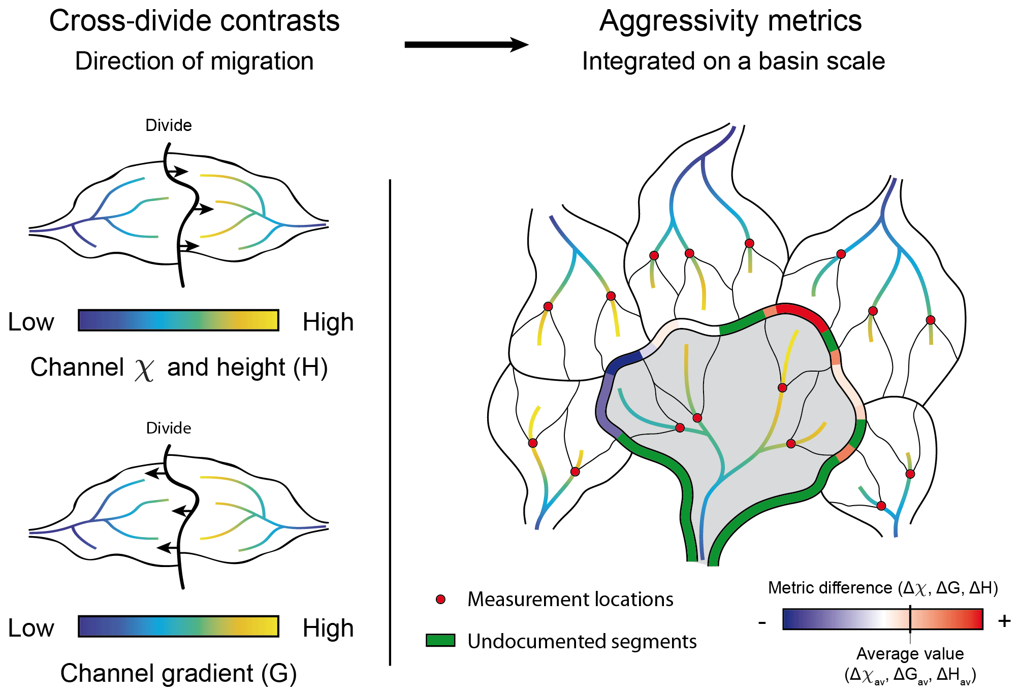
Figure 2 Conceptual relationship between cross-divide contrast in χ and Gilbert metrics and divide migration as exposed by Willett et al. (2014) and Forte and Whipple (2018). For χ and height, divides migrate toward the drainages that present higher values. For channel gradient, divides migrate toward the drainages that present lower values. In our study, channel χ, local gradient and height are measured at the outlet (indicated by red circles) of basins for a reference area (basins bounded with thin black lines). Aggressivity metrics are then calculated for a given basin (represented in grey) by averaging along its perimeter the individual cross-divide differences in metrics between reference basins. The proportion of perimeter which is not shared by two reference basins is measured to give a confidence index of the calculated aggressivity.

Then, we calculate the difference in metrics (Δχ, ΔG and ΔH) across the segments of divide shared by two reference basins. Finally, the aggressivity metric is obtained by averaging these cross-divide differences along the perimeter of each sampled basin (Fig. 2). This way, the sign of the aggressivity metric in a basin corresponds to the difference in the averaged value of considered metric difference (Δχ, ΔG and ΔH) in this basin with respect to its neighbours. This method has the advantage of weighting individual divide segments by the number of pixels they contain and then providing a robust assessment of the basin aggressivity. Aggressivity metrics based on χ, G and H are hereafter referred to as Δχ_av, ΔG_av and ΔH_av, respectively. However, due to topology issues, some parts of the perimeter of the sampled basins may be not shared by two reference basins (Fig. 2). We quantify this incompleteness by assessing the ratio of documented pixels over the total amount of pixel along the basin perimeter. We refer to this ratio as the “confidence index” CI, assuming that a higher CI is associated with a more robust basin aggressivity assessment.

3 Results

3.1 Evolution of reference model

A detailed analysis of the DEM suggests that during the initial phase, the flat initial surface (Fig. 3a) is progressively uplifted to form a plateau. At the same time the edges of this plateau are gradually regressively eroded by drainage networks that spread from the base level toward the centre of the model (Fig. 3b and c). This transient landscape is completely dissected after 2 Myr. From this time and until the end of the simulation, landscape changes are mainly due to competition between watersheds, resulting in continuous divide migrations with decreasing intensity as the model is moving toward a total topographic equilibrium (Fig. 3d–f; video no. 1 in the Supplement).

Figure 3 Map view of the temporal evolution of the reference model. Colour bar gives the model elevation. Black lines show the evolution – and the migration – over time of drainage divides for five drainage basins. Red circles in (e) and (f) show transient topography associated with drainage capture after 5 and 10 Myr of simulation, respectively (see video no. 1 in the Supplement).

To define the time period of regional steady state, we measure the average elevation, the maximum elevation and the average denudation rate over the entire model for each time step (Fig. 4a). We identify two distinct stages during the evolution of our reference simulation. During the first million years, due to long wavelength topographic building, the calculated landscapes are far from steady state. This leads to a major increase in the mean elevation from ca. 25 to ca. 75 m. In a second stage, this trend reverses and the mean elevation decreases asymptotically toward ca. 60 m until the end of the simulation.

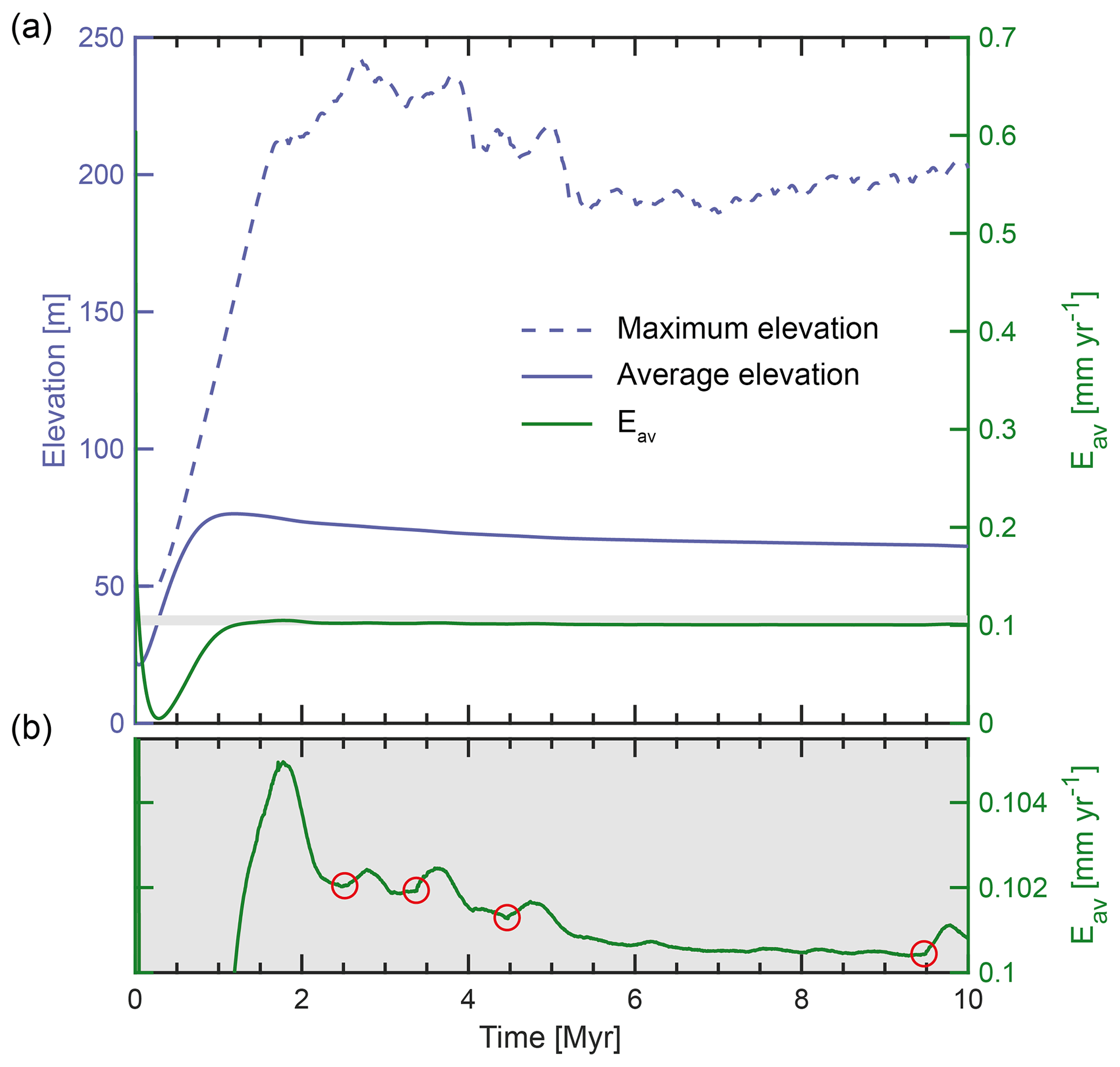
Figure 4 Evolution of the reference model over time. (a) Average elevation (solid blue line), maximum elevation (dashed blue line) and average denudation rate (solid green line) over the whole model. (b) Expanded view of the mean denudation rate of (a) (in the light grey area). Red circles highlight significant stream captures that lead to an abrupt increase in average denudation rates over a subsequent period of several time steps (effects associated with stream captures at 4.5 and 9.5 Ma are visible in Fig. 3e and f, respectively).

The evolution of the maximum elevation follows the same pattern but can be affected by temporal changes in the location and altitude of highest peaks. The maximum elevation increases between ca. 50 and ca. 250 m over the first 3 Myr (Fig. 4a) then decreases progressively to remain at ca. 200 m during the rest of the simulation.

We compute the average denudation rate from the rock uplift rate and from average elevation change over the entire model between two time steps:

$$\begin{array}{}\text{(5)}& {\left(\mathrm{\Delta }z/\mathrm{\Delta }t\right)}_{\mathrm{av}}=U-E_{\mathrm{av}},\end{array}$$

where (Δz∕Δt)_av is the average surface uplift over the entire model on a time-step Δt, U is the imposed uniform uplift rate (0.1 mm yr⁻¹) and E_av is the average “real” denudation rate. During the first 0.25 Myr, the mean denudation rate falls abruptly from ca. 0.6 mm yr⁻¹ to nearly 0 mm yr⁻¹ as a consequence of diffusion over the initial flat topography. After that time and until the first 1 Myr, the mean denudation rate increases but remains lower than the uplift rate, leading to the increase in average elevation over this time period. In the following 1 Myr, E_av exceeds the uplift rate to reach up to 0.104 mm yr⁻¹ before it gently decreases to 0.1 mm yr⁻¹ until the end of the simulation. This shows that topography tends to – but never reaches – a strict steady state over the simulation time. Abrupt changes in E_av after ca. 2.5, 3.5, 4, 5 and 9.5 Myr (red circles in Fig. 4b) are related to major local captures in the drainage network, which can be observed during the model evolution (red circles in Fig. 3e and f and video no. 1 in the Supplement).

Based on these results, we will consider that a regional topographic steady state is reached between 1.5 and 2 Ma, when the plateau relict topography is totally eroded and E_av begins to decrease (Figs. 3 and 4). This time is consistent with the time required to reach topographic steady state proposed from models with constant uplift rate and no horizontal advection (Willett et al., 2001).

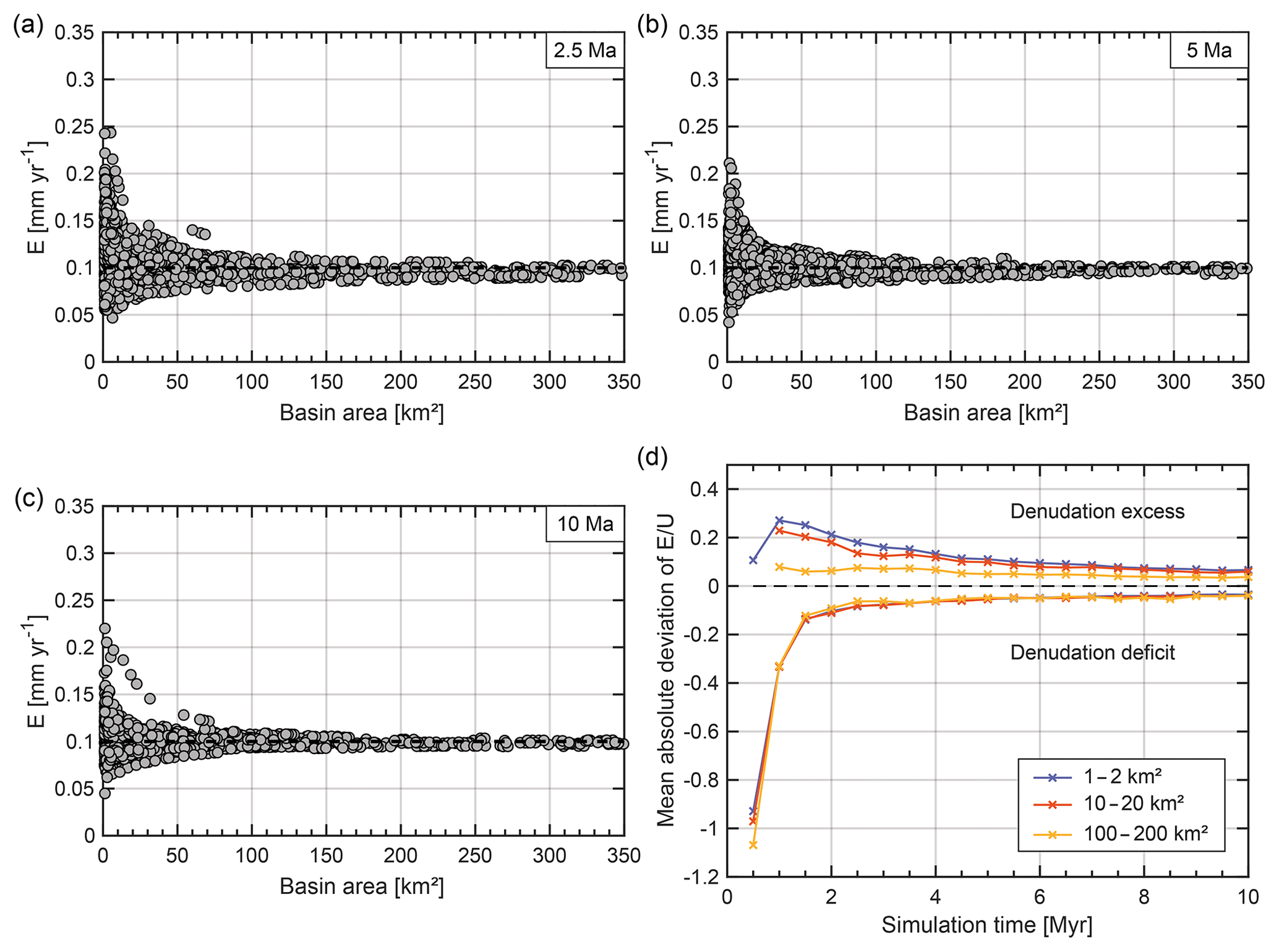
Figure 5 Variability of denudation rates over time for a compilation of five simulations of the reference model with different initial noised DEM. (a–c) Variability of denudation rate as a function of basin area after 2.5, 5 and 10 Myr of simulation, respectively. (d) Mean absolute deviation (MAD) from uplift rate (0.1 mm yr⁻¹) for three classes of basin sizes: 1–2, 10–20 and 100–200 km² between 0.5 and 10 Ma. Negative (positive) deviation is related to deficit (excess) of denudation.

3.2 Basin-wide denudation rates variability

We calculate basin-wide denudation rates E upstream of each stable drainage network confluence after 2.5, 5 and 10 Myr of simulation (Fig. 5a–c, respectively). Regardless of the duration, we observe a significant variability in the calculated denudation rates depending on basin size. As exposed by Forte and Whipple (2018), the erosion rate contrasts across divides are spatially limited to areas very near the divides. Thus, the variability is maximum for small basins (ca. 1 km²) and decreases with increasing basin area. In our approach, small basins are nested in larger ones. Hence, these results can be related to the averaging of denudation rates along the drainage network, in agreement with the measurements of Matmon et al. (2003b). This variability also decreases with time (Fig. 5a–c). For basins with an excess of denudation relative to the uplift rate U, the E∕U ratio can reach up to 2.5 after 2.5 Myr but only 2 after 5 Myr and 1.7 after 10 Myr. Basins with a denudation excess that stand out of the general trend at 10 Ma (Fig. 5c) are associated with a capture event visible in Fig. 4b. For basins with a deficit of denudation, the evolution of the ratio is less obvious. It can be lower than 0.5 after 2.5 Myr, but it increases slightly to 0.6 until 10 Myr. These results reflect a significant spatial variability of the difference between basin-wide denudation rates and uplift rate. To assess more accurately the temporal evolution of this variability, we calculate E every 0.5 Myr for three distinct categories of basin sizes: 1–2, 10–20 and 100–200 km². We then estimate the mean absolute deviation (MAD) from the uplift rate by considering separately basins with a denudation in excess or in deficit of uplift rate (Fig. 5d). Until 1.5 Ma, basins are located on the plateau where denudation rate is null. This leads to a low MAD for basins with a denudation deficit and to the absence of basins with a denudation excess. After 1.5 Ma, basins in deficit exhibit an increase in MAD from nearly −0.15 to −0.04 mm yr⁻¹, regardless of the area class considered. For basins in excess, the MAD value decreases through time, depending on drainage area: from ca. 0.25 to ca. 0.07 mm yr⁻¹ for basins with an area of 1–2 km², from ca. 0.2 to ca. 0.07 mm yr⁻¹ for basins of 10–20 km² and from ca. 0.7 to ca. 0.04 mm yr⁻¹ for the largest basins. We see a coherent evolution of this difference over the simulation time, consistent with the model progression toward topographic equilibrium.

The spatial variability of the denudation rates is neither homogeneous nor randomly distributed (Fig. 6a). The location of drainage basins with denudation rates far from the equilibrium value of 0.1 mm yr⁻¹ coincides with migrating drainage divides (Fig. 3d) and with cross-divide contrasts in channel χ, gradient and height (Fig. 6b–d). Following Willett et al. (2014) and Forte and Whipple (2018), the divide migrations predicted by these contrasts are consistent with the direction of divide mobility obtained from our model. One may note that the higher the contrast in these parameters across the divide, the higher the deviation of the denudation rate from the uplift rate, and therefore from topographic equilibrium. None of the sampled basins in this dataset contain a knickpoint. Thus, these results based on simulations assuming uniform and constant properties as well as constant boundary conditions confirm that the dispersion observed in denudation rates is primarily controlled by divide migration. Basins that expand (shrink) show higher (lower) denudation rates compared to uplift rate, and they are hereafter referred to as aggressors (victims), following the terminology adopted by Willett et al. (2014).

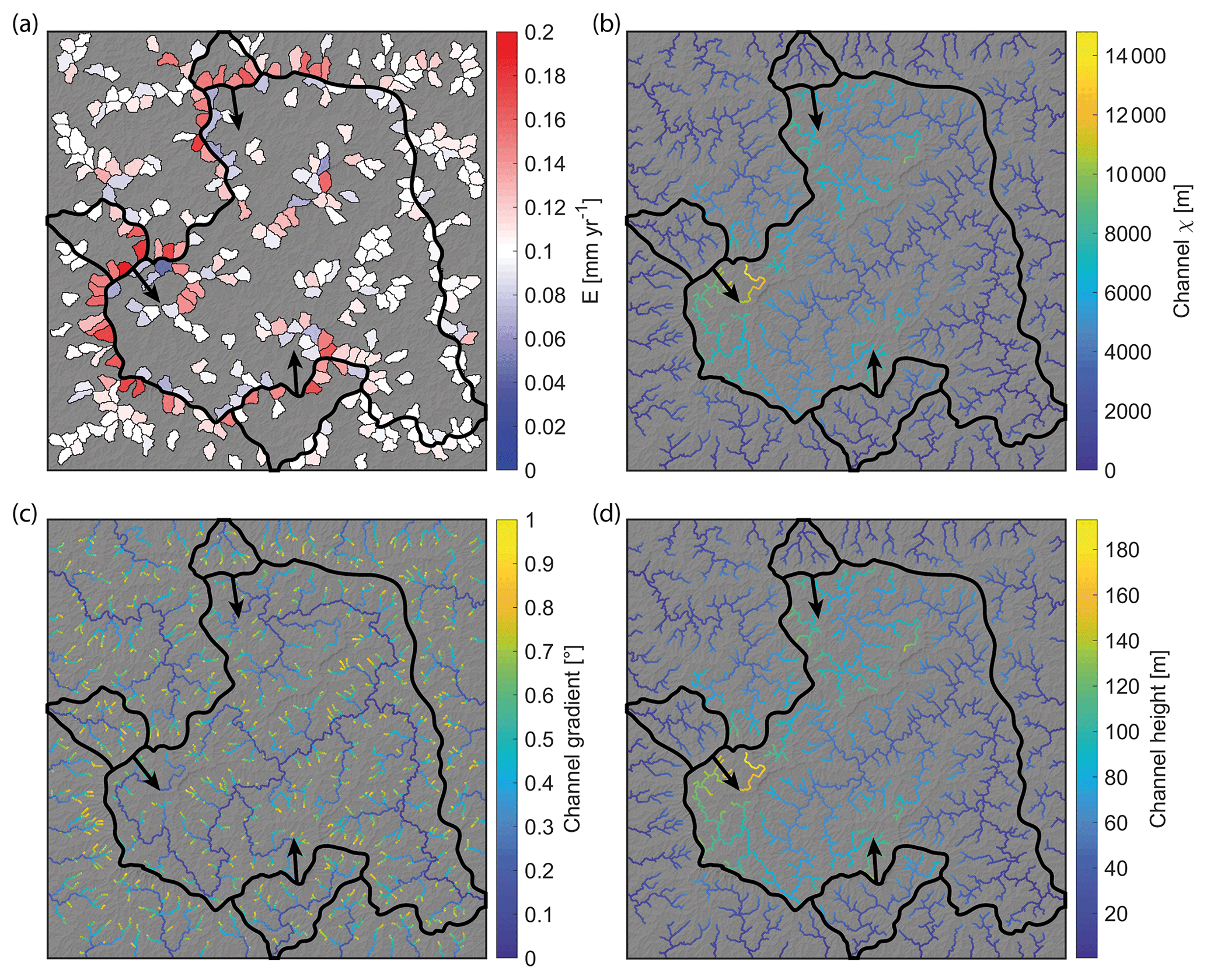
Figure 6 Denudation rates and cross-divide contrast metrics obtained for the reference model after 2.5 Myr of simulation. Drainage network is extracted from a minimal drainage area of 1 km². (a) Map of denudation rates for basins of 2–4 km². Thick black lines correspond to basin divides in Fig. 2d. Black arrows, show the direction of divide migrations for three selected basins; (b) χ map; (c) channel gradient map; (d) channel height map.

3.3 Deviation of denudation rates from the uplift rate and basin aggressivity

Willett et al. (2014) showed that the basin-averaged cross-divide contrast in χ, could be used to deduce an aggressivity metric for basins. We extend this basin-scale approach to the Gilbert metrics recently proposed by Forte and Whipple (2018) including cross-divide contrast in headwater gradient and elevation.

We here assess the relationship between the E∕U ratio and these aggressivity metrics. First, to exclude variability related to both basin area and time, we focus on a single class of basins with a size of 2–4 km² gathered from five computed reference models after a simulation duration of 2.5 Myr. Denudation rates may be affected by knickpoints, which are a source of transient perturbation at the scale of the catchment. Therefore, in order to focus only on perturbations associated with drainage divide dynamics, basins that contain knickpoints are ignored. In agreement with cross-divide metrics tested by Forte and Whipple (2018), graphs in Fig. 7 must be divided into four quadrants. Aggressor (victim) basins have negative (positive) Δχ_av and ΔH_av values and conversely a positive (negative) ΔG_av value (Fig. 2). Theoretically, aggressor (victim) basins have higher (lower) denudation rates than the underlying uplift rate. This result is verified for ca. 81 %, 52 % and 81 % of basins for Δχ_av, ΔG_av and ΔH_av, respectively. For this limited dataset, the evolution between E∕U and both Δχ_av and ΔH_av may be defined by a linear relationship (Fig. 7b). Compared to other metrics, ΔG_av is less sensitive to drainage migration and shows a more scattered distribution.

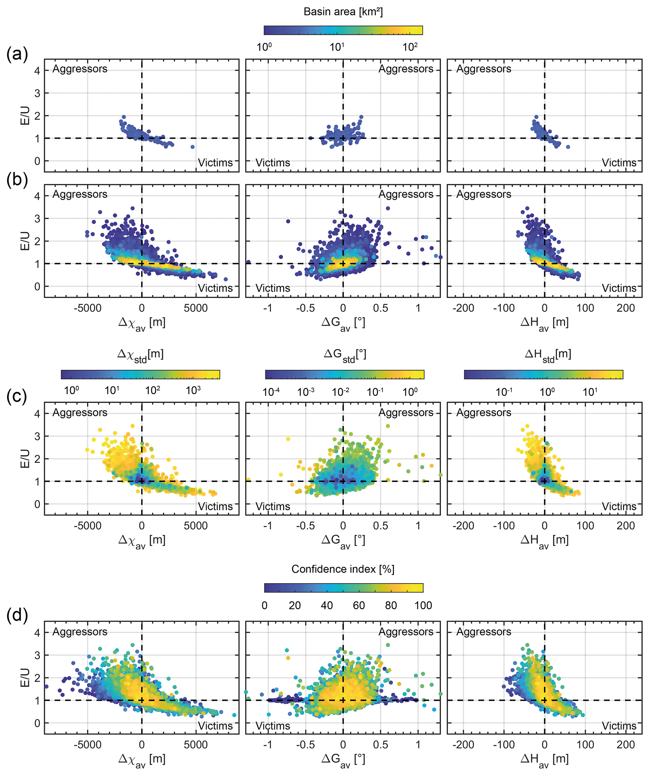
Figure 7 Denudation rates normalized by uplift rate as a function of aggressivity metrics and parameters influencing data dispersion. (a) Basins of 2–4 km² for the reference model after 2.5 Myr of simulation. Colour scale indicates basin area. Basins with a confidence index lower than 50 % are discarded from the analysis. (b) Basins of variable sizes are sorted into seven area classes expanding geometrically with a multiplying factor of 2 from 1–2 to 64–128 km², every 0.5 Myr over the time period 2–10 Myr. Colour scale indicates basin area. Basins with a confidence index lower than 50 % are discarded from the analysis. (c) Basin of 1–2 km² over the time period 2–10 Myr, colour scale indicating the standard deviation of Δχ, ΔG and ΔH, respectively. Basins with a confidence index lower than 50 % are discarded from the analysis. (d) Basin of 1–2 km² over the time period 2–10 Myr. Colour scale indicates confidence index.

In natural settings, the stage of evolution of landscapes cannot be easily defined and the total amount of basins with a specific size may be limited. The large dataset from our modelling can provide further insights by gathering the results obtained every 0.5 Myr for seven classes of basin areas expanding geometrically with a multiplying factor of 2 from 1–2 to 64–128 km² (Fig. 7b). Basins that contain knickpoints are discarded from the analysis. When all classes of drainage areas are combined together, we still obtain a clear relationship between aggressivity metrics and E∕U, with 77 %, 56 % and 78 % of basins lying in aggressor or victim quadrants for Δχ_av, ΔG_av and ΔH_av, respectively (Fig. 7b). Our results highlight the major control of basin size on the dispersion E∕U. Part of the variability intrinsic for each class of basin area may in turn be explained by heterogeneities in aggressivity between different parts of a basin. Figure 7c shows that this dispersion is related to the standard deviation of aggressivity metrics, Δχ_std, ΔG_std and ΔH_std. In other words, basins where different divide segments migrate at different rates or in different directions are more scattered. The lower the confidence index, the more scattered the results (Fig. 7d). Thus, some dispersion may come from approximations due to undocumented divide segments performed when averaging metric differences between reference basins (Fig. 2). One may note two different trends for victim and aggressor basins. Aggressors show a more scattered distribution for Δχ_av and ΔG_av metrics. When compared to victims, these basins have hillslopes closer to the critical value S_c (Fig. S3). Hence, the dispersion may be explained by the non-linear relationship existing between denudation rates and basin slope (Montgomery and Brandon, 2002; Binnie et al., 2007).

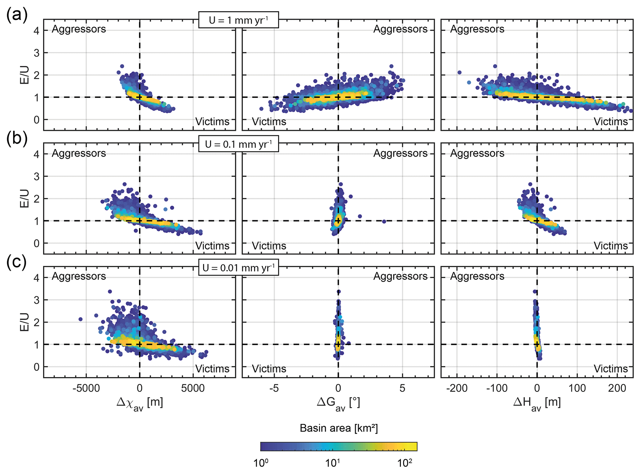
Figure 8 Sensitivity to uplift rates. Colour scale indicates basin area. Basins of variable sizes are sorted into seven area classes expanding geometrically with a multiplying factor of 2 from 1–2 to 64–128 km², every 0.5 Myr over the time period 5–10 Myr. Basins with a confidence index lower than 50 % are discarded from the analysis. (a) Results with an uplift rate of 1 mm yr⁻¹. (b) Results with an uplift rate of 0.1 mm yr⁻¹ (reference model). (c) Results with an uplift rate of 0.01 mm yr⁻¹.

4 Discussion

4.1 Sensitivity tests

The reference model involves various parameters related to uplift, fluvial incision and hillslope denudation. A systematic analysis of trade-offs between all parameters is out of the scope of this article. In this section, we assess the sensitivity of the results to both tectonic and erosion processes by studying the specific impact of uplift U, erodibility K, diffusivity D and critical hillslope gradient S_c taken separately. Varying these parameters may change the simulation time required to erode the plateau associated with the initial boundary conditions. In this section, to reduce sensitivity dependence on these initial conditions, we only consider results obtained between 5 and 10 Ma.

4.1.1 Sensitivity to uplift rate

We test rock uplift rates of 0.01, 0.1 (hereafter called reference model) and 1 mm yr⁻¹ to cover the range of a large variety of geodynamic settings (Champagnac et al., 2012). It is well known that a river responds to a fall in base level (due to changes in rock uplift rate or other forcing) by cutting downward into its bed, deepening and widening its active channel. In our simulations, changes in uplift rate lead to variations in the density of the drainage network. Compared to the reference model, an uplift rate of 1 mm yr⁻¹ (0.01 mm yr⁻¹) results in a decrease (increase) of drainage density. These results are consistent with previous studies that show an inverse relationship between drainage density and erosion rates in equilibrium topography when using a threshold slope for diffusion processes (Tucker and Bras, 1998; Clubb et al., 2016). An increase in uplift rate favours river entrenchment leading to an increase in the range of ΔG_av and ΔH_av (Fig. 8). Hence, these two Gilbert metrics appear to be well suited to diagnose local disequilibrium for higher uplift rates (i.e. ≥1 mm yr⁻¹). Conversely an increase in uplift rate induces a lower range of values for Δ χ_av. This last observation is explained by the decrease in drainage density and associated stream length.

Maximum variability of E∕U reaches a factor of 2, regardless of the assumed uplift rate between 1 and 0.01 mm yr⁻¹. The observed small differences suggest that limited uplift rates promote diffusive processes (see Sect. 4.1.3).

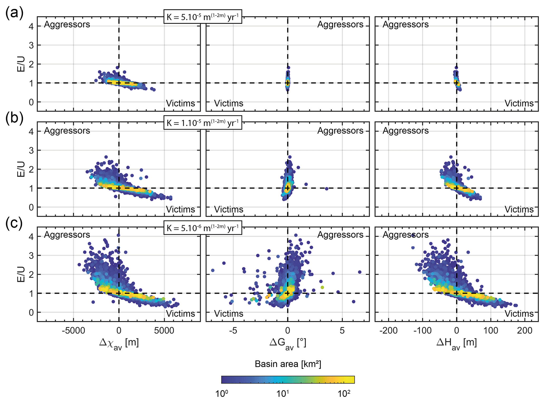
Figure 9 Effect of erodibility. Colour scale indicates basin area. Basins of variable sizes are sorted into seven area classes expanding geometrically with a multiplying factor of 2 from 1–2 to 64–128 km², every 0.5 Myr over the time period 5–10 Myr. Basins with a confidence index lower than 50 % are discarded from the analysis. (a) Results with an erodibility coefficient of $\mathrm{5}\times {\mathrm{10}}^{-\mathrm{5}}$ m^(1−2 m) yr⁻¹. (b) Results with an erodibility coefficient of $\mathrm{1}\times {\mathrm{10}}^{-\mathrm{5}}$ m^(1−2 m) yr⁻¹. (c) Results with an with an erodibility coefficient of $\mathrm{5}\times {\mathrm{10}}^{-\mathrm{6}}$ m^(1−2 m) yr⁻¹.

4.1.2 Influence of erodibility

Fluvial erosion is proportional to the erodibility coefficient K that may reflect, among others, rock strength and climate. We let this parameter vary between $\mathrm{5}\times {\mathrm{10}}^{-\mathrm{6}}$ and $\mathrm{5}\times {\mathrm{10}}^{-\mathrm{5}}$ m^(1−2 m) yr⁻¹. As expected from (Eqs. 1 and 3), we find that erodibility and uplift rates have opposite effects. Lower (higher) values of erodibility lead to higher (lower) average topography. Thus, an increase (decrease) in erodibility decreases (increases) the range of all aggressivity metrics (Fig. 9). Lower values of erodibility also increase the range of the E∕U ratio. Models with higher (lower) erodibility reach a quasi-topographic steady state earlier (at a later stage). Hence, differences in the variability of E∕U may be related to different stages of evolution for each model over the period we consider (5 to 10 Ma) (Fig. 5d).

4.1.3 Influence of hillslope processes

Hillslope denudation is proportional to the diffusivity coefficient D and depends on the critical slope S_c (Eq. 2). To test the effect of hillslope processes, we let D vary between 10⁻³ and 10⁻¹ m² yr⁻¹. Compared to the reference model, we find no differences in the case of a lower diffusivity (i.e. 0.001 m² yr⁻¹) (Fig. 10c). In contrast, for models with higher diffusivity coefficient (i.e. 0.1 m² yr⁻¹), this parameter has a significant effect on both the range of E∕U and the aggressivity metric ΔG_av (Fig. 10a). This result is consistent with the observations described in Sect. 4.1.1. It derives from a stronger impact of diffusive processes, which decrease local slopes in the vicinity of divides. In our modelling, the local slopes remain lower than the fixed critical value. Then, assuming a critical slope between 20 and 40^∘, we find that S_c does not affect significantly the relationship between the E∕U ratio and the studied metrics (Fig. 11).

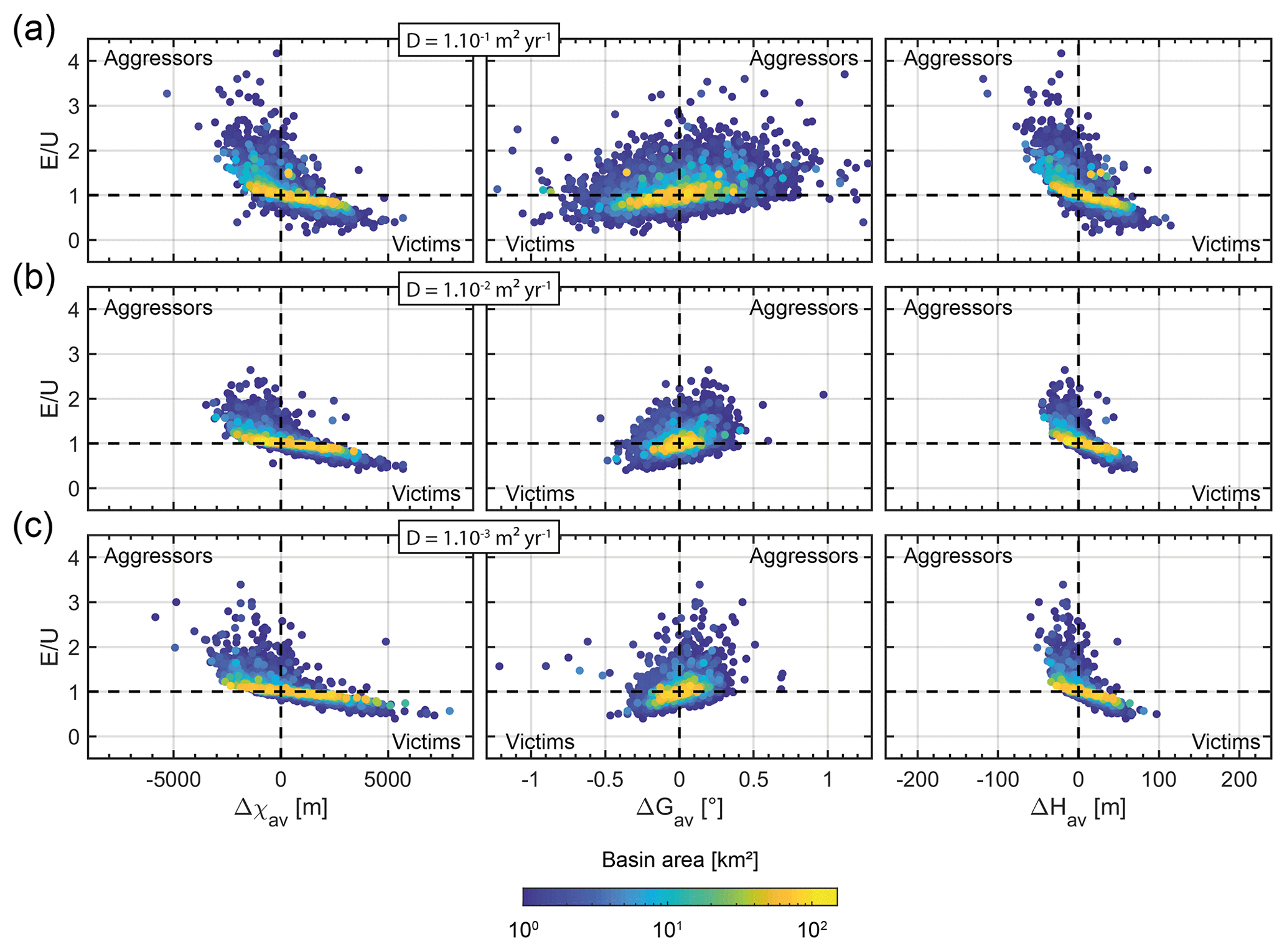
Figure 10 Effect of diffusivity. Colour scale indicates basin area. Basins of variable sizes are sorted into seven area classes expanding geometrically with a multiplying factor of 2 from 1–2 to 64–128 km², every 0.5 Myr over the time period 5–10 Myr. Basins with a confidence index lower than 50 % are discarded from the analysis. (a) Results with a diffusivity of 10⁻¹ m² yr⁻¹. (b) Results with a diffusivity of 10⁻² m² yr⁻¹ (reference model). (c) Results with a diffusivity of 10⁻³ m² yr⁻¹.

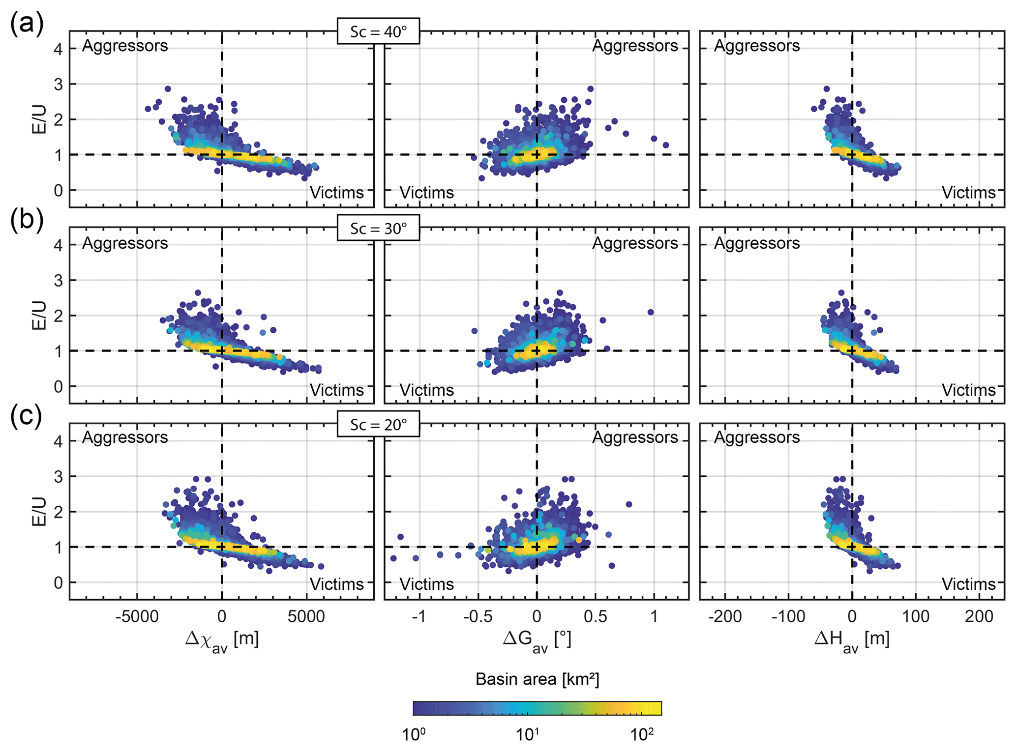
Figure 11 Effect of critical slope. Colour scale indicates basin area. Basins of variable sizes are sorted into seven area classes expanding geometrically with a multiplying factor of 2 from 1–2 to 64–128 km², every 0.5 Myr over the time period 5–10 Myr. Basins with a confidence index lower than 50 % are discarded from the analysis. (a) Results with a critical slope of 40^∘. (b) Results with a critical slope of 30^∘ (reference model). (c) Results with a critical slope of 20^∘.

Altogether, these sensitivity tests demonstrate the robustness of our findings. Regardless of the tested parameter values, we observe a relationship between aggressivity metrics and deviation of denudation rates from uplift rates. Thus, aggressivity metrics are, to the 1st-order, reliable metrics to assess the effect of divide mobility on basin-wide denudation rates inferred from simulations. In the following section, we apply this approach to field observations and discuss the consequences for sampling and interpretation.

4.2 Implications for the interpretation of basin-wide denudation rates

Over the last decades, measurements of cosmogenic radionuclide (CRN) concentrations in alluvial sediments (see Granger et al., 2013, and references therein), of suspended sediments (Gabet et al., 2008) and of detrital thermochronology (Huntington and Hodges, 2006) have become common practices to assess basin-wide denudation rates. However, their interpretation remains debated, even in settings where topographic steady state is supposedly achieved regionally.

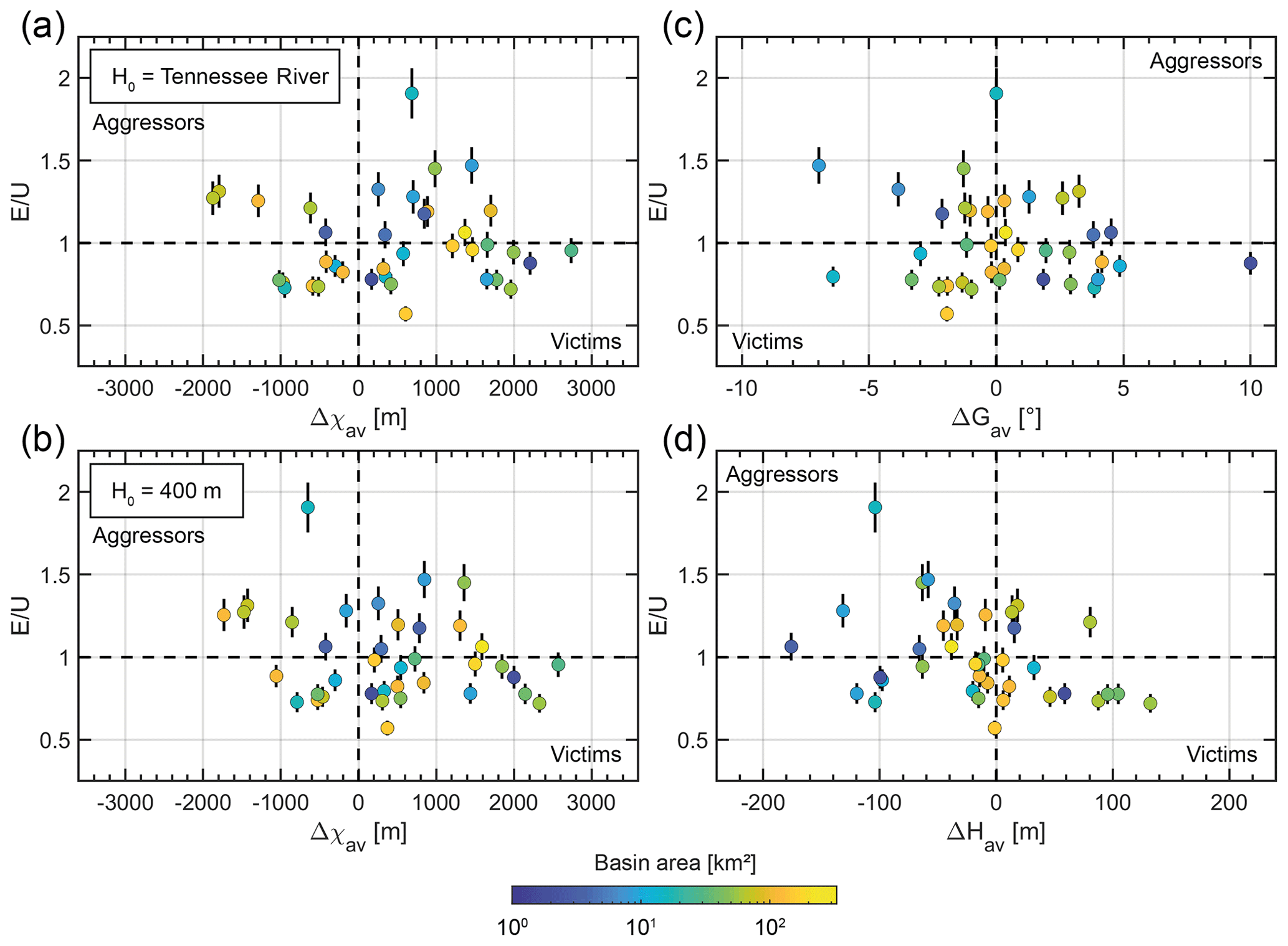
Figure 12 Normalized denudation rates in the Great Smoky Mountains as a function of aggressivity metrics. Original dataset from Matmon et al. (2003b) with E recalculated by Portenga and Bierman (2011). Denudation rates and uncertainties are normalized by the estimated background uplift rate in this region of 0.03 mm yr⁻¹. Error bars are represented with thin black line. Colour scale indicates basin size. (a, b) Relationship between denudation rates and Δχ_av with a base level corresponding to the Tennessee River and at a fixed elevation of 400 m, respectively. (c, d) Relationship between denudation rates and Gilbert aggressivity metrics, ΔG_av and ΔH_av, respectively.

4.2.1 Application to the Great Smoky Mountains

As previously mentioned (Matmon et al., 2003a, b), while the Great Smoky Mountains in the southern Appalachians are expected to be in a quasi-topographic steady state, basin-wide denudation rates show a strong dispersion up to a factor of 2 in comparison to the estimated uplift rate (ca. 0.03 mm yr⁻¹; see Fig. 1). We use the data associated with 40 basins originally sampled by Matmon et al. (2003a, b) and for which denudation rates were recalculated by Portenga and Bierman (2011). Following our method, we calculate the three basin-averaged aggressivity metrics Δχ_av, ΔG_av and ΔH_av associated with these 40 catchments (Fig. 12; see also Fig. S3). The calculation of χ requires us to define the elevation of the catchment outlets H_b and the m∕n ratio (Eq. 4). As underlined by Forte and Whipple (2018), the choice of the “correct” outlet elevation is non-trivial in natural settings. We first consider a local base level given by the Tennessee River. To test the relevance of this choice, we also use a base level located at a fixed arbitrary elevation H_b=400 m. We assume the same m∕n ratio value of 0.45 as used by Willett et al. (2014) for the Great Smoky Mountains. For all calculated metrics, the majority (ca. 58 % for ΔG_av and ca. 66 % for ΔH_av) of the basins is located in the expected quadrants (see Fig. 7). However, more attention must be given to the results based on Δχ_av. For this metric, ca. 58 % of the analysed basins lie in the expected quadrant when we consider the Tennessee River as the local base level versus ca. 68 % for H_b=400 m (Fig. 12b). Although the overall results are similar, we show that the choice of a different base level H_b leads to significant variations in Δχ_av for individual basins. This highlights the main weakness of the Δχ_av metric, which is highly sensitive to the choice of the proper base level H_b. Nevertheless, our results confirm the findings by Willett et al. (2014), suggesting that a significant part of the data variance observed in the Matmon et al. (2003a, b) can be explained by divide migration (Fig. 12), raising this possible explanation for the variability of most natural datasets. One may note that the southern Appalachians exhibit migrating knickpoints that can locally affect denudation rates (Gallen et al., 2011, 2013). This last point can also explain part of the observed variability in this dataset but this specific impact is beyond the scope of the present study.

Based on both our simulations and this field dataset, we propose favouring the use of Δχ_av and ΔH_av. Among the tested metrics, ΔG_av appears the least sensitive to disequilibrium, excepted in active mountain belts with rock uplift U≥1 mm yr⁻¹.

4.2.2 Assessment of topographic disequilibrium

Topographic steady state is a very convenient assumption and concept to deduce the uplift pattern in mountains ranges from denudation rates, and thus to obtain significant information on the geometry of active structures and on orogen dynamics (Lavé and Avouac, 2001; Godard et al., 2014; Scherler et al., 2014; Le Roux-Mallouf et al., 2015). However, this assumption is seldom verified at the scale of sampled watersheds.

On the basis of our modelling, we show that the competition between low-order basins has a significant impact on basin-wide denudation rates. The proposed approach provides a new tool to assess the potential deviation from topographic steady state based on aggressivity metrics and drainage area, which can both be inferred from a simple DEM: the closer to zero the aggressivity metrics and the lower the standard deviation of cross-divide metrics, the more representative of uplift rate the measured denudation rates.

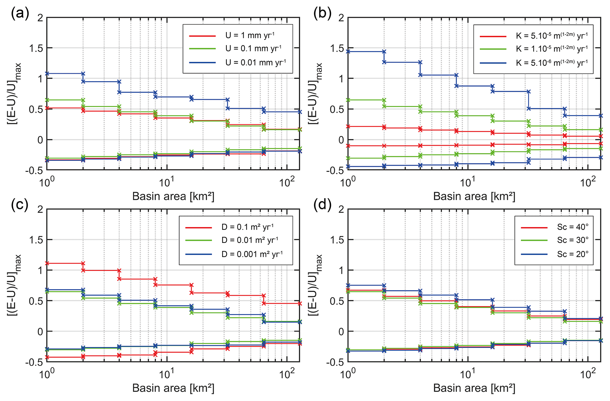
Figure 13 Deviation from steady state due to drainage migration as a function of basin size. Colour lines show the maximum dispersion of denudation rates (0.5 and 99.5 percentiles) due to divide mobility. Green lines indicate the reference model. Seven sets of basin size are considered: 1–2, 2–4, 4–8, 8–16, 16–32, 32–64 and 64–128 km² every 0.5 Myr between 5 and 10 Myr. (a) Effect of uplift rate. (b) Effect of erodibility. (c) Effect of diffusivity. (d) Effect of critical slope.

4.2.3 Improvement of sampling strategy

Basin-wide denudation rates obtained from CRN concentration measurements, suspended sediments or detrital thermochronology depend on many parameters including lithology, ice cover, rainfall, landslide activity or tectonic uplift (Vance et al., 2003; Bierman and Nichols, 2004; Wittmann et al., 2007; Yanites et al., 2009; Norton et al., 2010; Godard et al., 2012; Whipp and Elhers, 2019). Hence, to unravel the influence of tectonics from other processes, a specific sampling strategy is usually recommended: (1) to sample catchments with homogeneous lithologies to limit the effect of spatial variations in the abundance of target minerals in bedrock formations; (2) to select catchments with no ice cover (past or present) because the input of glacier-derived sediments can significantly complicate the interpretation of CRN concentrations; (3) to choose areas with spatially uniform rainfall distribution; and (4) to consider watersheds where the relative contribution of landslides to long-term landscape evolution is low. Unfortunately, these different criteria imply selection of watersheds with variable sizes. The first three criteria favour the sampling of small catchments, whereas the last one requires basins large enough to be less affected by landslides.

Our approach suggests the need to pre-assess targeted basins for their potential divide mobility before sampling for CRN concentration measurements. If the objective is to quantify the background uplift rate, one should sample basins that satisfy the conditions we previously described in the current section and also display an aggressivity close to zero and with the smallest associated standard deviation. Conversely, to quantify the specific denudation rate associated with the migration of drainage divides, small aggressor or victim basins should be favoured.

Based on our simulations, a relationship between the maximum of erosion variability (0.5 and 99.5 percentiles, respectively) due to divide mobility $\left[\right(E-U)/U{]}_{\max }$ and the catchment size A can be derived (Fig. 13). Our results suggest a logarithm dependence between these two parameters, regardless of the assumed U, K, D and S_c:

$$\begin{array}{}\text{(6)}& \left[\right(E-U)/U{]}_{\max }=c_{\mathrm{1}}\log (A)+c_{\mathrm{2}}\mathrm{for}\mathrm{1}{\mathrm{km}}^{\mathrm{2}}<A<\mathrm{100}{\mathrm{km}}^{\mathrm{2}},\end{array}$$

with c₁ and c₂ being two parameters that depend on the balance between erosion processes, uplift rate and state of evolution of the landscape.

5 Conclusions

Calculations from a landscape evolution model assuming spatially uniform uplift, rock strength and rainfall confirm that the concept of topographic steady state is relevant at the scale of entire mountain belts, but this represents an oversimplification at the scale of individual watersheds. Our simulations underline the role of divide mobility on deviations from equilibrium, which can lead to significant differences between tectonic uplift rate and basin-wide denudation rates even if an overall topographic steady state is achieved at large scale.

To better assess these deviations, we propose new basin-averaged aggressivity metrics – Δχ_av, ΔG_av and ΔH_av – based on the approach by Willett et al. (2014) and Forte and Whipple (2018). They include mean cross-divide contrasts in channel χ, local gradient and height. From our calculations, Δχ_av is the most reliable aggressivity metric to assess local disequilibrium, but it is highly dependent on the chosen base level, which remains hard to constrain. Gilbert metrics ΔG_av and ΔH_av are more suitable for relatively high uplift rate (i.e. ≥1 mm yr⁻¹). Altogether, our metrics reveal that deviation of denudation rates from uplift rate related to divide migrations depends on both basin aggressivity and basin area. This last parameter has a key control on the dispersion in E∕U, which can reach a factor of 2, regardless of the imposed uplift rate (here 0.01–1 mm yr⁻¹), erodibility (here $\mathrm{5}\times {\mathrm{10}}^{-\mathrm{6}}$–$\mathrm{5}\times {\mathrm{10}}^{-\mathrm{5}}$ m^(1−2 m) yr⁻¹), diffusivity (here 10⁻³–10⁻¹ m² yr⁻¹) or hillslope gradient (here 20–40^∘). By comparing our results to CRN measurements from the Great Smoky Mountains (Matmon et al., 2003a, b), we show that this approach can be used to improve field sampling strategies and provides a new tool to derive a minimal uncertainty in basin-wide denudation rates due to topographic disequilibrium.

For the sake of simplicity our models involve spatially homogenous and time invariant parameters. Additional simulations are now needed to test this approach in more complex settings, including spatial and temporal variability in climate and tectonic forcing or parameters like stream power equation exponents n and m.