Potential erosion capacity of gravity currents created by changing initial conditions

We investigate to what extent the initial conditions (in terms of buoyancy and geometry) of saline gravity currents flowing over a horizontal bottom influence their runout and entrainment capacity. In particular, to what extent the effect of the introduction of an inclined channel reach, just upstream from the lock gate, influences the hydrodynamics of gravity currents and consequently its potential erosion capacity is still an open question. The investigation presented herein focuses on the unknown effects of an inclined lock on the geometry of the current, on the streamwise velocity, on bed shear stress, and on the mechanisms of entrainment and mass exchange. Gravity currents were reproduced in the laboratory through the lock-exchange technique, and systematic tests were performed with different initial densities, combined with five initial volumes of release on horizontal and sloped locks. The inclination of the upstream reach of the channel (the lock) was varied from 0 % to 16 %, while the lock length was reduced by up to 1∕4 of the initial reference case. We observed that the shape of the current is modified due to the enhanced entrainment of ambient water, which is the region of the current in which this happens most. A counterintuitive relation between slope and mean streamwise velocity was found, supporting previous findings that hypothesized that gravity currents flowing down small slopes experience an initial acceleration followed by a deceleration. For the steepest slope tested, two opposite mechanisms of mass exchange are identified and discussed, i.e., the current entrainment of water from the upper surface due to the enhanced friction at the interface and the head feeding by a rear-fed current. The bed shear stress and the corresponding potential erosion capacity are discussed, giving insights into the geomorphological implications of natural gravity currents caused in different topographic settings.

1 Introduction

Gravity currents are common phenomena that may occur spontaneously in nature or triggered by human activities. These flows are created by differences in hydrostatic pressures at the surface of contact of two fluids that have different densities. Examples of gravity currents generated in the atmosphere are katabatic winds, which are created by temperature inhomogeneities that originate the density gradient. Avalanches of airborne snow and plumes of pyroclasts from volcanic eruptions are atmospheric flows wherein suspended particles play a major role in producing the density gradient. If suspended sediment produces the extra density, gravity currents are called turbidity currents. Turbidity currents have received major attention, since the sedimentation they induce due to the high amount of sediments they transport has important economic costs related to the loss of volume for water storage (Palmieri et al., 2001; Schleiss et al., 2016). Among gravity currents caused by human actions, the release of pollutants into rivers, oil spillage in the ocean and desalination plant outflows are of primary importance due to their negative environmental impacts.

Gravity currents have been the subject of research over the last decades. Simpson (1997), Kneller and Buckee (2000), Huppert (2006), and Ungarish (2009) present a comprehensive review of the early work on natural and experimentally reproduced gravity currents. Recently, Azpiroz-Zabala et al. (2017) provided a new model for the gravity current structure. They argued that real-world turbidity currents in submarine canyons are characterized by a so-called “frontal cell”, which is highly erosive and therefore able to be self-sustaining and to outrun the slower-moving body of the flow, creating a stretched current. Nevertheless, authors working on small-scale experimentally reproduced gravity currents agree on describing the shape of the gravity current as composed by an arising highly turbulent front, called the head, followed by, in some cases, a body and a tail. The difference between the two concepts mainly comes from the observation timeframe, which is of the order of hours for experimentally reproduced gravity currents, while it is of days for the observations that Azpiroz-Zabala et al. (2017) made in Congo Canyon.

Within the body, which can reach a quasi-steady state, a vertical structure can be distinguished. A gravity current presents two main interfaces at which exchanges concur: at the bottom, generally a solid boundary, and at the top, at the interface with the ambient fluid. These are active boundaries at which mass and momentum exchanges are promoted (Ancey, 2012). Ambient fluid is entrained due to shear and buoyancy instabilities at the upper interface (Cantero et al., 2008), resulting in the dilution of the underlying current and modification of the density profile that characterizes a gravity current under stable density stratification (Turner, 1973). If the gravity current travels above an erodible bed, entrainment of material from the bottom can take place, which is conveyed with the current and sometimes redeposited at large distances from the original position (Zordan et al., 2018a). High shear stress associated with intense ejection and burst events influences erosion and bed load transport (Niño and Garcia, 1996; Cantero et al., 2008; Zordan et al., 2018a). For example, in the shallow shelf region of the lake it is frequently observed that cold water, which is relatively denser than that in open waters, starts to descend down the slope as a cold gravity current (Fer et al., 2002). The plume is able to transport suspended sediment together with the dissolved components, oxygen and pollutants into deeper water. A proper parameterization of both upper-layer and bottom entrainment is still an open research field that needs to be addressed. Indeed, small variations in entrainment highly influence flow dynamics (Traer et al., 2012).

Due to instabilities at the interface with the ambient fluid, the current entrains the lighter fluid and therefore it dilutes. Lock volume and lock slope are initial trigger conditions of experimentally reproduced gravity currents, and the main objective of the paper is to understand their influence on the transport capacity of the flows. We show how shear stress at the boundaries is dependent on the conditions under which a gravity current forms, i.e., its initial and boundary conditions. Different initial conditions, representing configurations that can possibly be found in nature, are tested by varying the initial volume of denser fluid and the lock geometry.

Gravity currents are reproduced here in the laboratory by the lock-exchange technique. Three initial densities are tested in combination with five lock lengths on a horizontal bottom and with four inclinations of the upstream channel reach. The bottom of the channel was designed in order to have a variable slope angle of the lock and a following flat surface. We were in search of a threshold at which an inversion of the leading forces of these currents would occur, which are gravitational forces and friction at the upper interface with the ambient fluid. Previous studies mainly focused separately on either low slopes or large slopes, missing the analysis of the transition that is tested here thanks to a specific experimental setup that allows for a wider range of configurations. Finally, we use a parameter previously defined in Zordan et al. (2018a) for the evaluation of the bottom erosion capacity as a surrogate to evaluate the influence of each different trigger condition on the erosion capacity of the currents.

Britter and Linden (1980) reproduced gravity currents down a slope with no breaks and found a critical angle, which is typically less than a degree, over which buoyancy force is large enough to counteract the bottom friction, producing a steady flow. At larger slopes, two mechanisms affect the evolution of the current: the current entrains water from the upper surface due to the enhanced shear stress, and the head is fed by the rear steady current. Mulder and Alexander (2001) studied slope-break deposits created by turbidity currents. They said that the amount of mixing between flow and ambient fluid is influenced by slope changes, which furthermore cause significant changes in turbidite thickness. In the present study the effect of a change in slope is analyzed by testing a range of lock slopes below 16 % ($\mathrm{0}{}^{\circ }\le \mathit{\alpha }<\mathrm{9}$^∘). It is expected that the two mechanisms mentioned by Britter and Linden (1980) will take place in the lock for the depletion current formed here due to the incremental gravitational forces, so a transition occurs from a friction-governed flow to a flow in which gravitational forces become more and more important. The erosion potential of a gravity current formed under such varying initial conditions is then discussed.

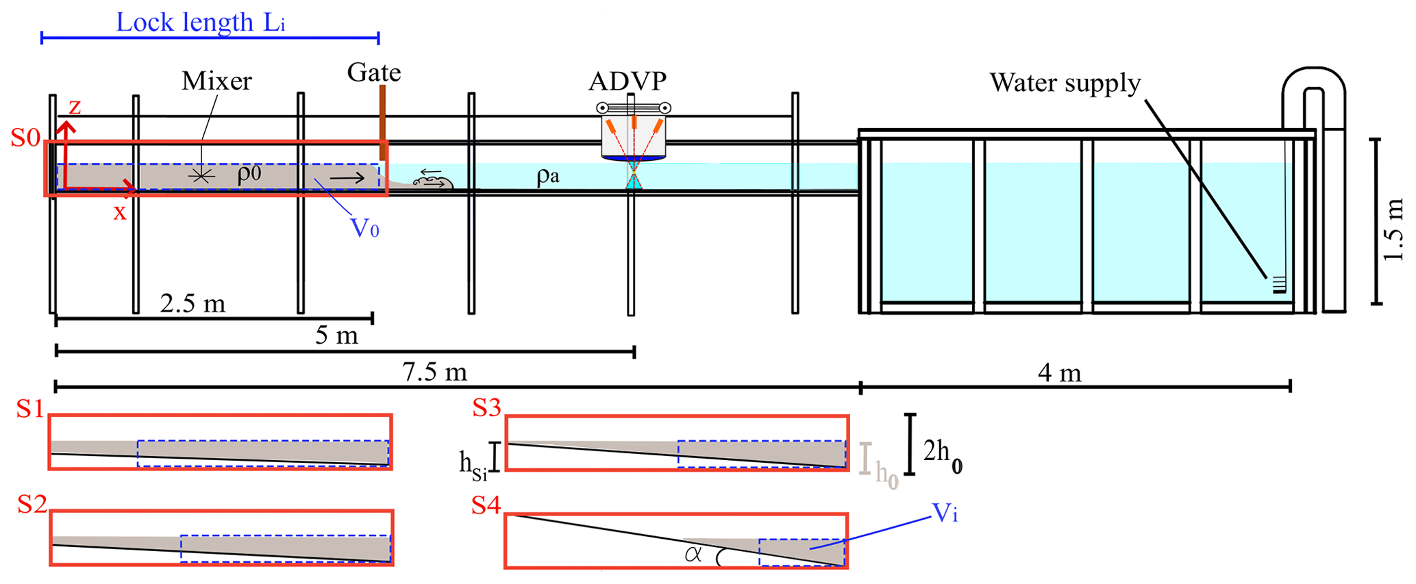
Figure 1 Longitudinal view and cross section of the experimental setup showing tested slope configurations S0 to S4 of lock volumes V_i.

The present paper is structured as follows: first, the experimental setup and the process that allows for the noise reduction of the velocity measurements are described. Then, the results are presented: a method for the identification of the shape of the current is described and, by means of the mean streamwise velocity field, both bottom and interface shear stresses are computed. The variation in the shape caused by changing initial conditions (i.e., with different initial buoyancies, various lock lengths and lock-bottom inclinations) is therefore discussed. The potential water entrainment and bottom erosion capacity are estimated on the basis of the computed shear stresses evolutions. Finally, an overview of the main findings is presented in the conclusions.

2 Methodology

2.1 Experimental setup

The tests are performed in a channel with a rectangular section 7.5 m long and 0.275 m wide. The gravity currents are reproduced through the lock-exchange technique by the sudden release of a gate that divides the flume in two parts whereby the fluids of different densities are at rest. Three buoyancy differences are tested in combination with five lock slopes ranging from S=0 % (horizontal bed) to S=16 % (tests S0 to S4). Figure 1 shows the configurations from a horizontal bed (S0) to the steepest slope (S4). By introducing a slope on the channel lock reach, the volume of denser fluid is reduced. This lock contraction is also tested separately by performing reference tests with the combination of the three initial densities and the five lock lengths that correspond to the very same volumes in the lock of the tests under inclined conditions. The experimental parameters are reported in Table 1. R_i–S_i refers to gravity currents reproduced by different initial densities with the presence of a lock slope, while R_i–L_i indicates the tests with varying initial density and lock length.

The channel is filled with 0.2 m of ambient water in one side and salty water, up to the same level, in the lock reach. Once the gate is removed, the saline current forms. At 2.5 m from the gate an acoustic Doppler velocity profiler (ADVP) is placed to measure 3-D instantaneous velocities along a vertical. The ADVP (Lemmin and Rolland, 1997; Hurther and Lemmin, 2001; Franca and Lemmin, 2006) is a nonintrusive sonar instrument that measures instantaneous velocity profiles using the Doppler effect without the need for calibration and was used with an acquisition frequency of 31.25 Hz. The velocity profiles are collected in time along a fixed vertical. The flume is connected to a final big reservoir that allows the current to dissipate and avoids its reflection upstream.

Normalization of the time is made using the scale $t^{*}=h_{\mathrm{b}}/u_{\mathrm{b}}$, where h_b is a vertical geometric scale, considered here as one-third of the total height of the fluid in the experimental tank, h₀ ($h_{\mathrm{b}}=h_{\mathrm{0}}/\mathrm{3}$ and h₀=0.2 m) and $u_{\mathrm{b}}=\sqrt{g^{\prime }{h}_{\mathrm{b}}}$ is the buoyancy velocity.

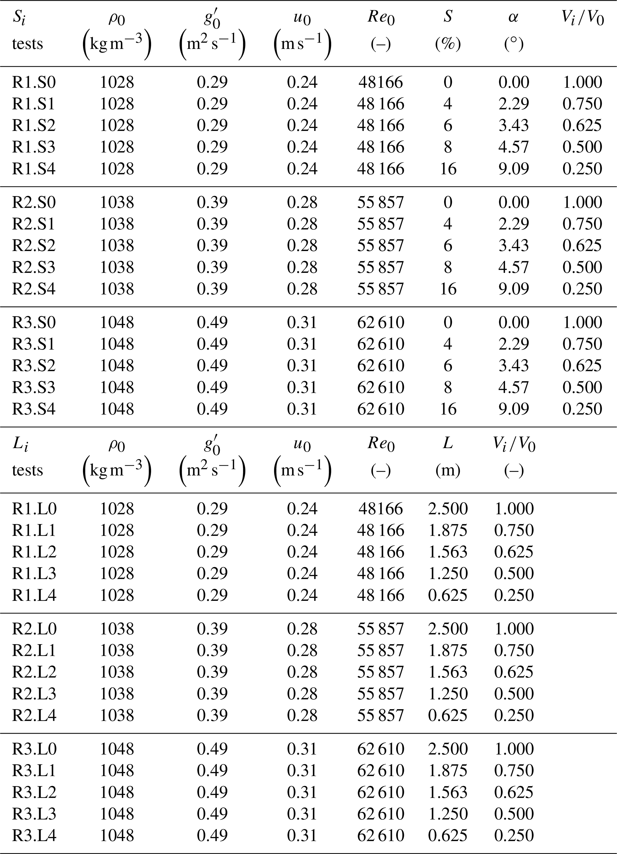
Table 1 Experimental parameters. ρ₀ is the initial density of the mixture in the upstream tank (measured with a densimeter), g^′ is the reduced gravity corresponding to ρ₀, $R{e}_{\mathrm{0}}=u_{\mathrm{0}}{h}_{\mathrm{0}}/{\mathit{\nu }}_c$ is the Reynolds number based on initial quantities with $u_{\mathrm{0}}=\sqrt{g^{\prime }{h}_{\mathrm{0}}}$ the initial buoyancy velocity, h₀=0.2 m is the total height of the water column, ν_c is the kinematic viscosity of the denser fluid, α is the angle of inclination of the bottom in the lock, S is the lock slope expressed in percentage ($h_{S_i}/L_{\mathrm{0}}$, with $h_{S_i}$ the height as in Fig. 1), L_i is the length of the upstream lock reach and V_i∕V₀ is the percentage of volume of the upstream lock reach with respect to the configuration L₀.

2.2 Data filtering

By means of an analysis of the power spectra of the raw data collected with the ADVP, noisy frequencies were mainly detected below 8 Hz. The instantaneous measurements were thus low-pass filtered with 8 Hz as a cutoff frequency (Zordan et al., 2018a). The 8 Hz cutoff has been chosen because the signal, for frequencies higher than 8 Hz, showed white noise. Time series of the mean streamwise and vertical velocities ($\stackrel{\mathrm{‾}}{u}$ and $\stackrel{\mathrm{‾}}{w}$) for the unsteady gravity current were derived after a filtering procedure that consisted of the application of a moving average over a time window that is chosen through the analysis of the power spectra distribution as in Baas et al. (2005). This analysis showed that for a time window of 0.32 s, the harmonics of all the meaningful frequencies were still recognizable, while by increasing the time window, the harmonics of progressively smaller frequencies gradually lose power and become impossible to distinguish (Baas et al., 2005). Thus, this window length was chosen for the moving average defining $\stackrel{\mathrm{‾}}{u}$ and $\stackrel{\mathrm{‾}}{w}$. The turbulent fluctuation time series (u^′ and w^′) is then calculated using the Reynolds decomposition:

$$\begin{array}{}\text{(1)}& u=\stackrel{\mathrm{‾}}{u}+u^{\prime },\end{array}$$

where u is the instantaneous velocity. The cleaning procedure with the velocity signals and corresponding spectra is shown in Fig. 2.

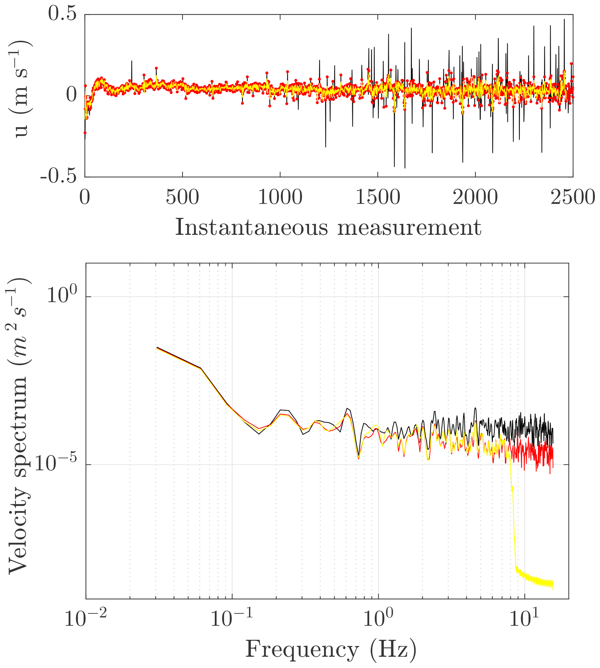
Figure 2 Raw velocity data (black) and despiked data (red) obtained with the procedure proposed by Goring and Nikora (2002). Then, through the analysis of the velocity spectra (bottom), the cutoff frequency of 8 Hz has been identified in order to low-pass filter the noisy frequencies (yellow line).

3 Results

3.1 The shape of the current

A criterion to identify the two main regions of a gravity current, the head and the body, is established here. Inspired by Nogueira et al. (2014), who considered the product of the depth-averaged streamwise velocity with the depth-averaged density of the current, we decide to adopt a similar procedure but taking into account the velocity field and the shape as relevant characteristics for distinguishing between the head and body. These distinctive features (a characteristic velocity and the contour of the current) have therefore been used in order to define a function that allows us to universally identify those regions of the currents. The kinematic function (H) is computed as the product between the instantaneous depth-averaged streamwise velocity, u_d(t),

$$\begin{array}{}\text{(2)}& u_{\mathrm{d}}\left(t\right)={\displaystyle \frac{\mathrm{1}}{h}}\underset{\mathrm{0}}{\overset{h}{\int }}u(z,t)\mathrm{d}z,\end{array}$$

and the current height, h(t), that is identified here by the position at which the streamwise velocity is equal to zero, as in Zordan et al. (2018a). H is thus defined as

$$\begin{array}{}\text{(3)}& H\left(t\right)=u_{\mathrm{d}}\left(t\right)h\left(t\right).\end{array}$$

By dimensional analysis, the function H corresponds to a flow rate per unit width. The head of the gravity current is characterized by a high specific flow rate that decreases at the rear of the head, a region in which fluid is recirculated through vortical movements.

Here, L_h identifies the temporal extension of the head and it is identified by the first meaningful local minimum of the function H, starting from the front. The conversion from time to length scale may be done by using the Taylor frozen hypothesis and considering a reference velocity of the current velocity as advection velocity. This method is coherent for all the experiments performed, and the value of the H function is shown in Fig. 3.

The body length is analyzed by using the cumulative sum of the function H. This is a region in which a quasi-steady regime is established for a certain time length. This implies that ∑H shows a linear increment in time. The limit of the body is therefore defined by analyzing the linear evolution that is fitted by a linear regression with a least squares method for progressively longer portions of the accumulated summed data. The analysis of the development of the R² value, the coefficient of determination, allows us to find the extension of the linear portion that corresponds to the temporal extent of the body region (L_b). R² is defined as the square of the correlation between the response values and the predicted response values. It is computed as the ratio of the sum of squares of the regression (SSR) and the total sum of squares (TSS) as

$$\begin{array}{}\text{(4)}& R^{\mathrm{2}}={\displaystyle \frac{\mathrm{SSR}}{\mathrm{TSS}}}={\displaystyle \frac{{\displaystyle }\sum _{i=\mathrm{1}}^n(y_i-{\widehat{y}}_i{)}^{\mathrm{2}}}{{\displaystyle }\sum _{i=\mathrm{1}}^n(y_i-{\stackrel{\mathrm{‾}}{y}}_i{)}^{\mathrm{2}}}},\end{array}$$

where $\stackrel{\mathrm{‾}}{y}$ is the average of the response y, $\widehat{y}$ is the regression line and n the number of observations i. In Fig. 3 the development of the function H is shown for the tests with the lock slope.

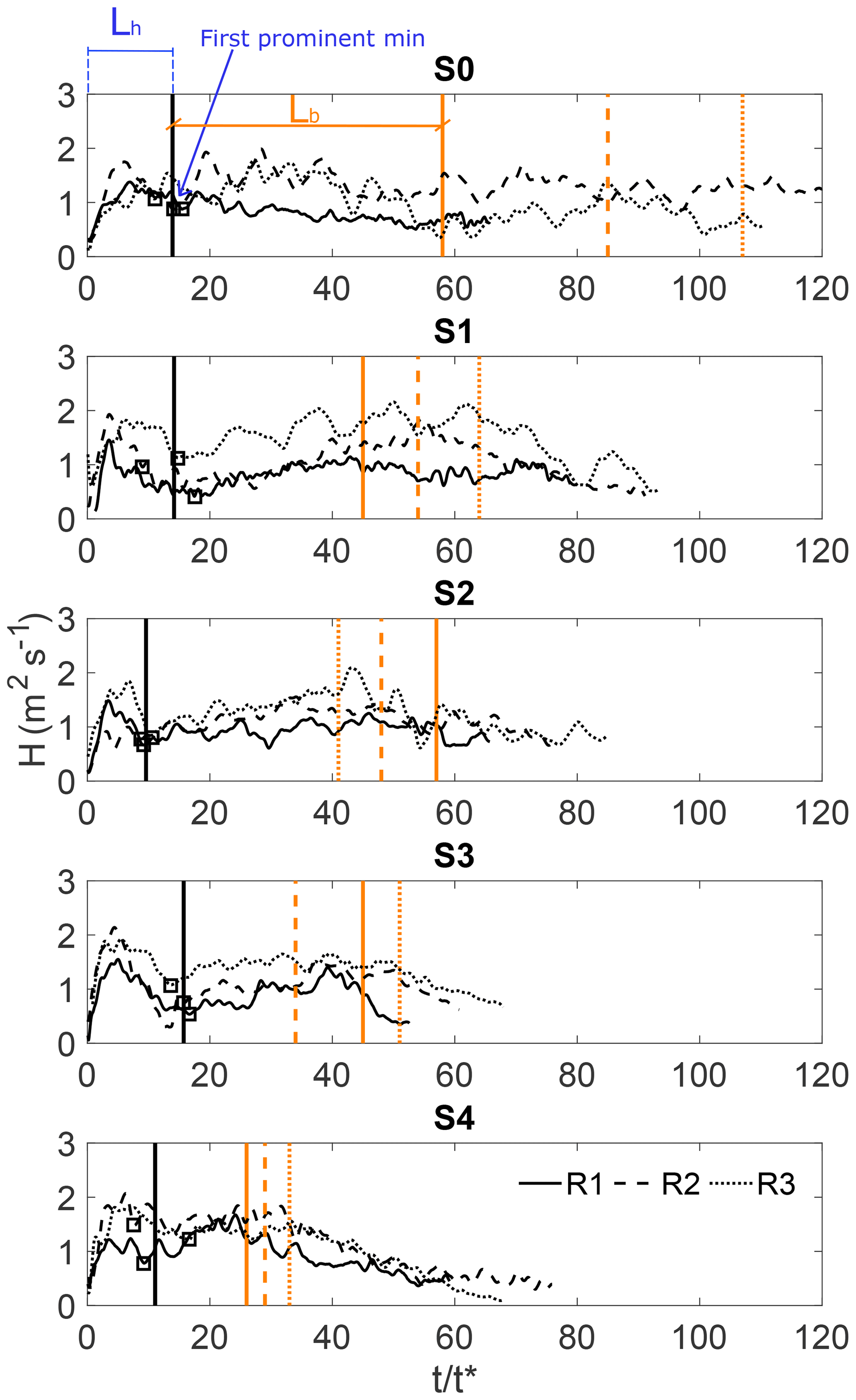
Figure 3 Determination of the gravity current head extension from the first prominent minimum of the function H (L_h). The extension of the body (L_b), as identified by the cumulative sum of the depth-averaged streamwise velocity, is also traced with the red vertical lines.

The same procedure is adopted for tests R_i.L_i, and the results can be found in Zordan et al. (2018b).

The form of the currents was identified by the zero streamwise velocity contour. In Fig. 4 the contours of each test with the lock slope are compared with the correspondent reference test with lock-length variation. The results are grouped by the initial density on the lock (columns in the figure) and by pairs of tests with the same volume of the lock but for different slopes. The extension of the head and body as identified by previous methods is also reported with the vertical lines. Dashed lines refer to tests S_i, while continuous lines correspond to L_i tests.

In Fig. 4 we can see that the head of the currents does not show any relevant change. Instead, the extension of the body is affected: it is reduced with an increasing inclination of the upstream channel reach and the same goes for tests produced by reduced lock volume. A dependency on the initial density is noticed, and three out of the total five slopes lead to the formation of a longer body with greater initial buoyancy. This can be verified in Fig. 3 where extensions of the bodies are plotted with the vertical orange lines. R1, R2 and R3 produce progressively longer bodies for tests S0, S1 and S4.

The largest deviation between the two contours of corresponding tests L_i–S_i is noticed for the last configuration, with the R_i–L4 tests showing a shorter body and a more defined tail, while for the correspondent tests with the inclined lock the body is more extended.

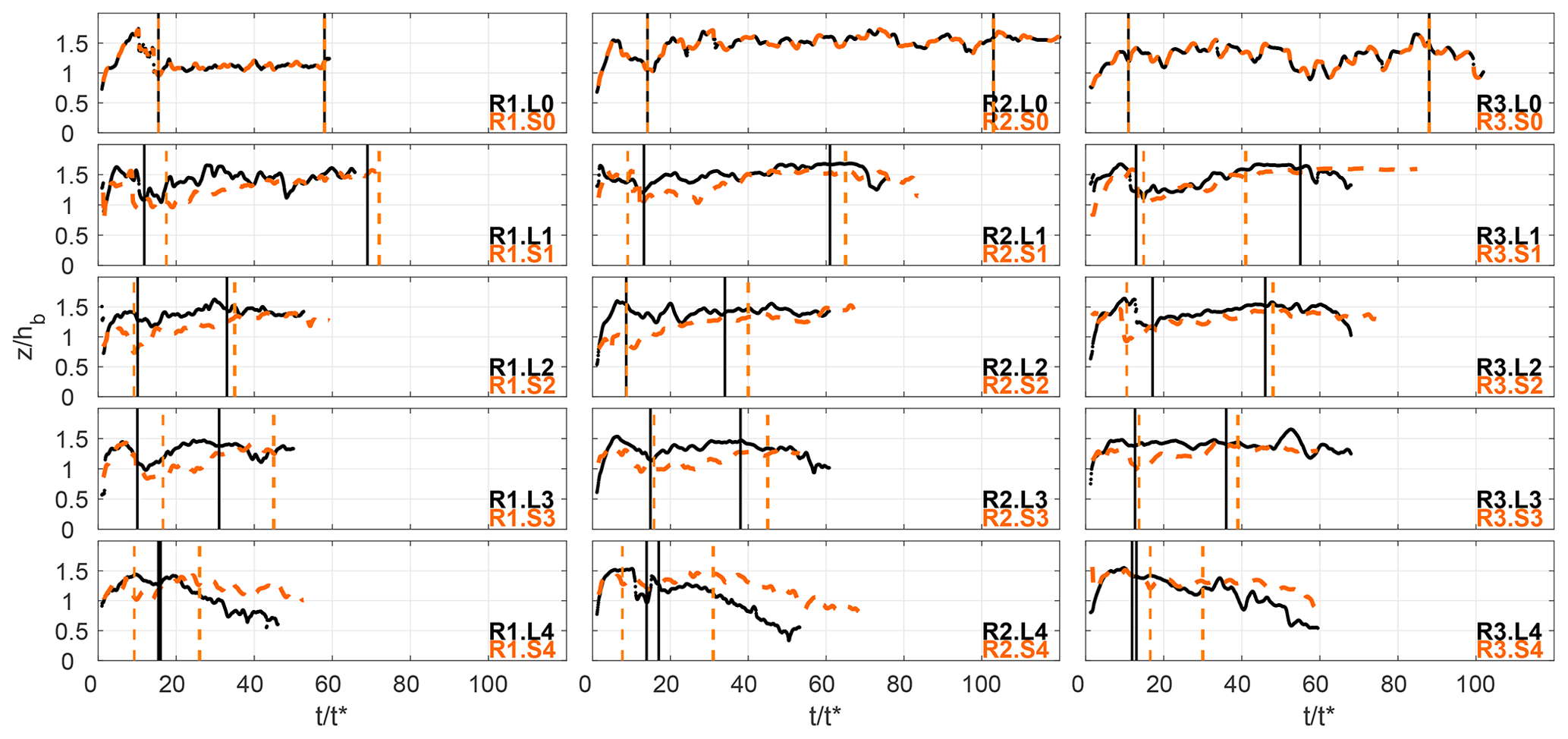
Figure 4 Gravity current contours, as identified by the zero streamwise velocity contour, for tests with the lock slope and correspondent tests with lock-length variation.

3.2 Mean velocity field

In Fig. 5 the mean streamwise velocity field on the background and velocity vectors of the components ($\stackrel{\mathrm{‾}}{u}$, $\stackrel{\mathrm{‾}}{w}$) are shown for all the tests performed. The heads of the currents are indicated by the vertical dashed lines, and the zero streamwise velocity contours are marked by the black lines. We can notice that the structures of the currents are quite similar in all configurations. An arising head is followed by a zone of high mixing, characterized by the presence of billows (due to Kelvin–Helmholtz types of instabilities; Simpson, 1972) that are due to shear at the rear part of the elevated head. The body and tail are not always well-defined regions, mainly for the class of tests down an incline, and therefore the contour is not drawn. Moreover, tests S_i show lower streamwise velocities within the head and body with respect to correspondent L_i tests.

By comparing tests S_i with the correspondent L_i tests, which have the same lock volume but are performed without upstream slope, it is noticed that mean streamwise velocity is slightly higher for tests on a horizontal bed. This can appear to some extent contradictory, but that behavior has already been mentioned in the literature in the study of Beghin et al. (1981), who were among the first to investigate the role of the slope on the physics of a gravity current. They showed that test flows on small slopes, for tests in which the entire channel was inclined (typically less than 5^∘), experience a first acceleration phase followed by a deceleration phase. This is because of the fact that, although the gravitational force increases as the lock slope becomes more inclined, there is also increased entrainment, both into the head itself and into the flow behind. This produces an extra dilution of the current with a decrease in buoyancy.

3.3 Bottom and upper shear stress

The sedimentological impact of a gravity current is the result of the complex hydrodynamics of this flow. Sediment entrainment is a complex mechanism mainly due to the difficulty in defining the fluctuating nature of turbulent flow (Salim et al., 2017). In Zordan et al. (2018a) the transport of sediment within a gravity current is linked to bed shear stress, which is considered here to be a “surrogate” measure of it. The fact that bed shear stress is affected by the changing initial conditions of the current thus explains how the entrainment capacity of a current is altered. Bed shear stress temporal evolution is calculated by following the procedure in Zordan et al. (2018a) in which it was assumed that the mean flow met the conditions necessary for the fitting of the overlapping layer by the logarithmic law of the wall as (Ferreira et al., 2012)

$$\begin{array}{}\text{(5)}& {\displaystyle \frac{\stackrel{\mathrm{‾}}{u}\left(z\right)}{u_{*}}}={\displaystyle \frac{\mathrm{1}}{k}}\ln {\displaystyle \frac{z}{z_{\mathrm{0}}}},\end{array}$$

where $\stackrel{\mathrm{‾}}{u}\left(z\right)$ is the mean velocity, u_* is the friction velocity, which is the velocity scale corresponding to the bed shear stress (Chassaing, 2010), k is the von Kármán constant, z is the vertical coordinate and z₀ is the zero velocity level.

The equation of the logarithmic law of the wall can be rewritten as

$$\begin{array}{}\text{(6)}& u=A\ln \left(z\right)-B,\end{array}$$

where

$$\begin{array}{}\text{(7)}& A={\displaystyle \frac{u_{*}}{k}},B={\displaystyle \frac{u_{*}}{k}}\ln \left(z_{\mathrm{0}}\right).\end{array}$$

Then, by determining the coefficients A and B through a fitting procedure, one obtains an estimation of u_*, which is the velocity scale corresponding to the bed shear stress.

Bed shear stress is afterwards computed by considering a constant initial density that is equal here to the initial density in the lock (ρ₀):

$$\begin{array}{}\text{(8)}& {\mathit{\tau }}_{\mathrm{b}}={\mathit{\rho }}_{\mathrm{0}}{u}_{*}^{\mathrm{2}}.\end{array}$$

The fitting procedure of the bottom logarithmic layer was determined stepwise by extending a linear least squares fitting range (in a semilogarithmic scale) from the lowest measured point until the point along the vertical of maximum streamwise velocity. Then, within this region, the sublayer that provided the best regression coefficient was chosen and considered for the estimation of u_*, corresponding to the extent of the logarithmic layer as was shown in Zordan et al. (2016).

The flow boundary is assumed to be smooth by verifying that the shear Reynolds number (or skin roughness, k_s, normalized by the viscous layer) is less than 5 (Nezu et al., 1994):

$$\begin{array}{}\text{(9)}& {\displaystyle \frac{k_{\mathrm{s}}{u}_{*}}{\mathit{\nu }}}\le \mathrm{5}.\end{array}$$

The classic value of the von Kármán constant of k=0.405 is adopted. A discussion of the estimation of k can be found in Ferreira (2015).

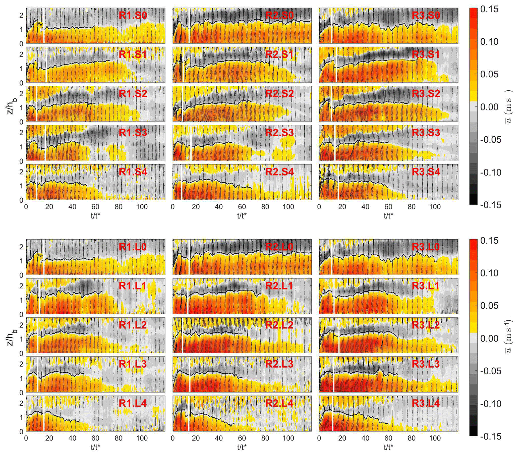
Figure 5 Streamwise velocity field on the background and velocity vectors of the components (u, w). The head of the current is delimited by the vertical white line. The contour of the current is indicated in black.

The bed shear stress time evolution of gravity currents with lock slope (τ_b,S) is compared to the analogous results for tests with decreasing lock (τ_b,L). Therefore, the time-averaged bed shear stress has been computed and the ratio $\stackrel{\mathrm{‾}}{{\mathit{\tau }}_{\mathrm{b},\mathrm{L}}}/\stackrel{\mathrm{‾}}{{\mathit{\tau }}_{\mathrm{b},\mathrm{S}}}$ is shown in Fig. 6. Tests performed with a lock slope show on average lower values of bed shear stress ($\stackrel{\mathrm{‾}}{{\mathit{\tau }}_{\mathrm{b},\mathrm{L}}}/\stackrel{\mathrm{‾}}{{\mathit{\tau }}_{\mathrm{b},\mathrm{S}}}\ge \mathrm{1}$). By increasing the lock slope this tendency is less evident and the mean bed shear stress is comparable for both conditions with varying lock slope and with different lock lengths. Moreover, tests performed with the highest density difference seem less affected by a changing configuration (S_iL_i with $i=\mathrm{1},\mathrm{2},\mathrm{3},\mathrm{4}$). The detailed time series for this condition are presented in Fig. 8, where we can see that from normalized time $t/t^{*}\simeq \mathrm{20}$, i.e., in the body region, bed shear stress is slightly higher for tests S_i than in the correspondent L_i tests.

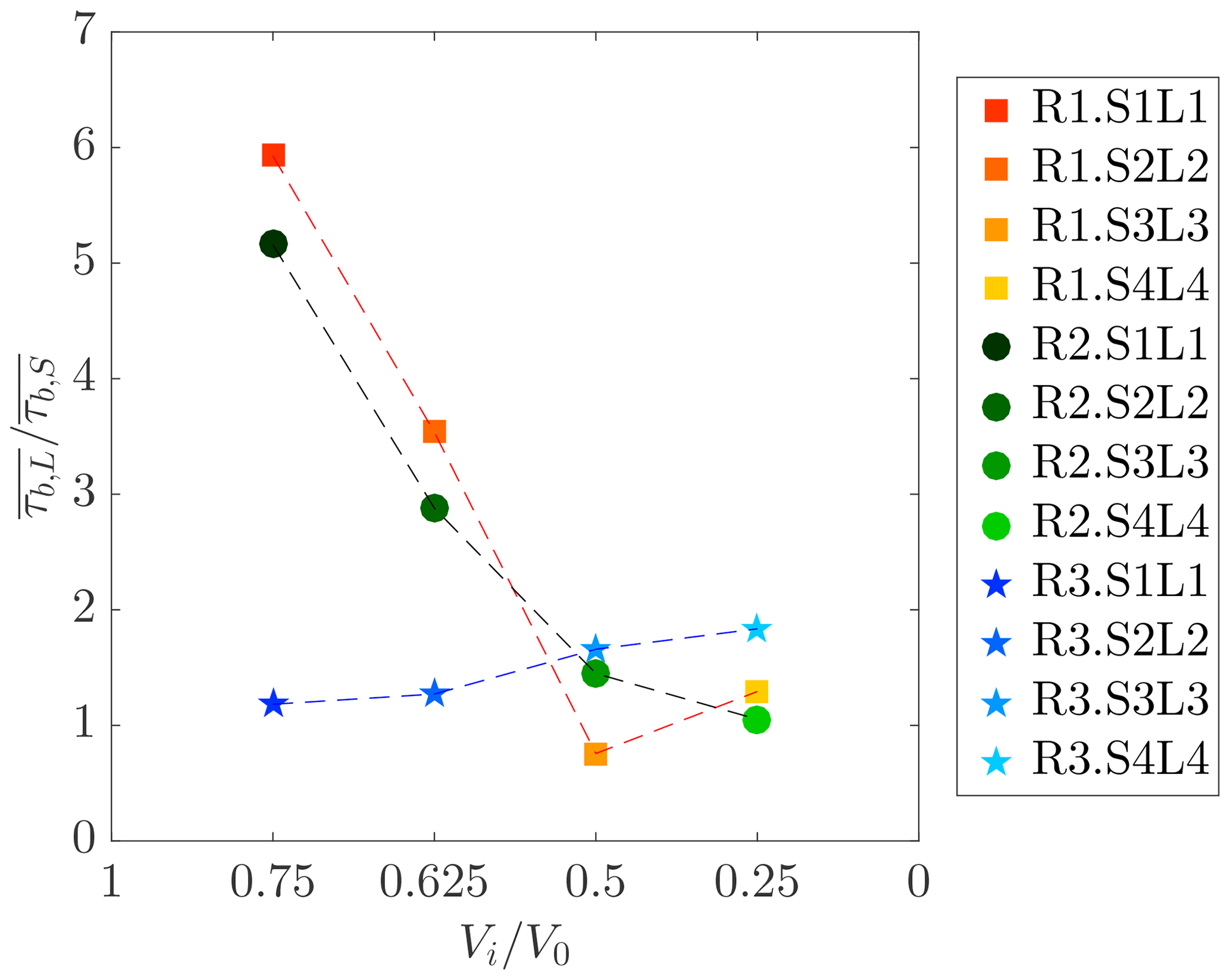
Figure 6 Ratio between time-averaged bed shear stress of tests with varying lock lengths ($\stackrel{\mathrm{‾}}{{\mathit{\tau }}_{\mathrm{b},\mathrm{L}}}$) and test with varying lock slopes ($\stackrel{\mathrm{‾}}{{\mathit{\tau }}_{\mathrm{b},\mathrm{S}}}$) versus percentage of volume of the upstream lock reach V_i∕V₀. Dashed lines link tests performed with the same initial excess density.

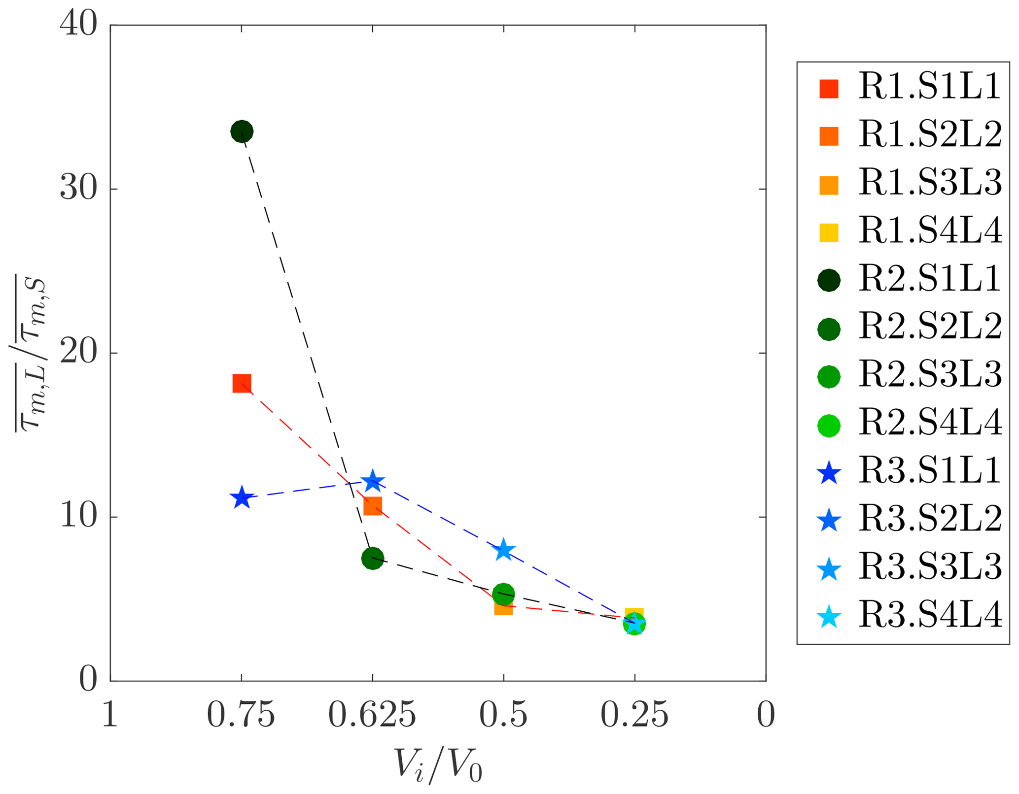
Figure 7 Ratio between time-averaged interface shear stress of tests with varying lock lengths ($\stackrel{\mathrm{‾}}{{\mathit{\tau }}_{\mathrm{m},\mathrm{L}}}$) and test with varying lock slopes ($\stackrel{\mathrm{‾}}{{\mathit{\tau }}_{\mathrm{m},\mathrm{S}}}$) versus percentage of volume of the upstream lock reach V_i∕V₀. Dashed lines link tests performed with the same initial excess density.

At the upper boundary of the gravity currents, i.e., the interface with the ambient water, studies on turbulent flow near a density interface confirmed that under certain conditions, the turbulent boundary layer theory can be applied as well (Lofquist, 1960; Csanady, 1978) and that the “law of the wall” can be used to estimate the shear stress here. By hypothesizing a constant mean value of water viscosity and hydraulically smooth conditions, the estimation of an interface shear stress (τ_m) is made; qualitatively, the estimation that will result is enough for the purpose of the present study. The time evolution of interface shear stress is therefore computed following the same procedure as for the bottom shear stress. In this case the fitting procedure of the logarithmic layer is determined by considering the mixing layer as defined in Zordan et al. (2018b). This layer is delimited at the top by the zero streamwise velocity contour and at the bottom by the height of the current as defined by the Turner's integral scales (Ellison and Turner, 1959). Within this layer, the (at least three) consecutive measurement points along the velocity profile that were giving the highest R² were considered for fitting. The time average of the interface shear stress is compared by means of the ratio $\stackrel{\mathrm{‾}}{{\mathit{\tau }}_{\mathrm{m},\mathrm{L}}}/\stackrel{\mathrm{‾}}{{\mathit{\tau }}_{\mathrm{m},\mathrm{S}}}$ (Fig. 7), showing that in general tests performed with varying lock lengths present higher values with respect to correspondent tests with lock-slope variation, i.e., $\stackrel{\mathrm{‾}}{{\mathit{\tau }}_{\mathrm{m},\mathrm{L}}}/\stackrel{\mathrm{‾}}{{\mathit{\tau }}_{\mathrm{m},\mathrm{S}}}\ge \mathrm{1}$.

Again, the main differences between tests with reduced lock and respective tests with lock slope are for the fourth configuration, detailed time series of which are shown in Fig. 9. The steepest slopes present higher values of interface shear stress in the body region with respect to the correspondent tests with the same initial volume of release but flowing on a horizontal bed.

4 Discussion

4.1 Shape variation of gravity current with the lock slope

The extensions of the body of correspondent tests performed with the lock slope or with a horizontal bed and with varying lock lengths are compared in Fig. 10. For lower lock slopes the body extension is similar to the currents produced with the same lock volume but with a horizontal bottom. However, for lock slopes at 16 %, the body region for tests S_i is longer than correspondent tests L_i. At this point two mechanisms affect the evolution of the current: the current entrains water from the upper surface due to the enhanced friction at the interface between the denser flow and the counter-current progressively advancing upwards the lock, and the head is fed by the rear current. The flow of tests S4 show that the characteristics of the upstream flow in the lock are influencing the flow even when the current reaches the measuring point: (i) an extended body is the result of water entrainment at the upper surface of the current that creates dilution and expansion of the fluid in the current; and (ii) the fluid in the body becomes faster as a result of the gravitational forces as in Britter and Linden (1980) (Fig. 5). Britter and Linden (1980) showed that for currents flowing along a horizontal boundary, the head is the controlling feature. However, down a slope, the body becomes more determinant in the gravity current evolution since it is up to 30 %–40 % faster than the head velocity, depending on the slope, therefore being able to move faster fluid into the head. In our study, the lock slopes at 16 % show those features, and the effect is not only occurring within the inclined lock but is also observed in the downstream flat part of the channel.

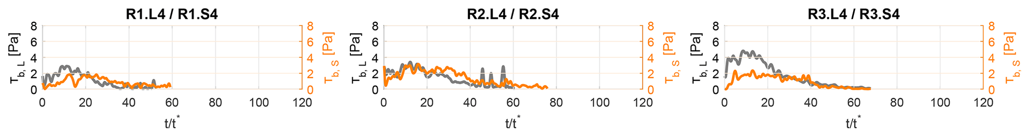
Figure 8 Temporal evolution of bed shear stresses calculated by log-law fitting for tests with progressively reduced lock length (τ_b,L) and with the lock slope (τ_b,S).

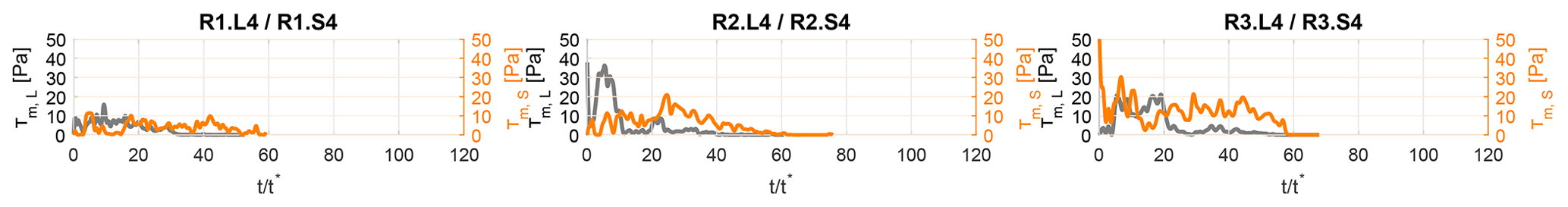
Figure 9 Temporal evolution of interfacial shear stresses calculated by log-law fitting for tests with progressively reduced lock length (τ_m,L) and with the lock slope (τ_m,S).

4.2 Ambient fluid entrainment

Kelvin–Helmholtz instabilities have a major role in provoking water entrainment. They take the form of vortical movements generated due to velocity shear at the interface between the two fluids. Since shear stress is determinant in the process of water entrainment, a new quantity to account for the potential entrainment capacity of the gravity current is defined here on the basis of the computed time evolution of the interfacial shear stress (τ_m). It is computed as the nondimensional time integral of the shear stress that represents, after dimensional analysis, the work done over a determined duration per unit surface for a given advection velocity, which can be approximated as the initial buoyancy velocity, u₀. This quantity Φ_m is calculated as

$$\begin{array}{}\text{(10)}& {\mathrm{\Phi }}_m=\underset{T_{\mathrm{1}}}{\overset{T_{\mathrm{2}}}{\int }}{\mathit{\tau }}_{\mathrm{m}}\left(t\right)\mathrm{d}t/t^{*},\end{array}$$

where the limits of integration are T₁=L_h and T₂=L_b in order to focus on the body, the region that has been found to be most affected by the variation of the initial conditions. The validity of the use of Φ_m as an indicator of the entrainment capacity is supported by the analysis of its relation with the Richardson number Ri (Zordan et al., 2018b). The relation between water entrainment and bulk Richardson number is well known in the literature and numerous empirical fits to the experimental data have been proposed since the early work of Parker et al. (1987) and supported by the more recent contributions of Stagnaro and Pittaluga (2014). Since bulk Richardson number is based on depth-averaged quantities, it assumes that properties do not vary significantly along the vertical. The quantity Φ_m, a surrogate for entrainment capacity, relies on instantaneous measurements of shear stress and therefore accounts for the unsteady behavior of the currents. Therefore, it is proposed here to use this quantity as a surrogate for water entrainment capacity since it benefits from instantaneous measurements of shear stress and it accounts for the unsteady behavior of the gravity currents. In Fig. 11, the potential water entrainments for gravity currents performed on an incline and correspondent tests with a reduced initial volume of release are compared. The tests R_i.S4 and R_i.L4 detach from the identity line, and thus a greater water entrainment is expected for the case with the inclined bed with respect to the horizontal bottom. The enhanced entrainment that has been verified for gravity currents formed downstream of steep slopes is due to the shear at the interface with the ambient water. According to Beghin et al. (1981), gravity currents are experiencing two phases while flowing along the channel. An initial acceleration takes place due to higher gravitational forces, and then the current accelerates, inducing an increment of shear stresses at the interface. The entrainment of clear water is therefore intensified and the currents are diluted. At the point at which the measurements are taken, the gravity currents are experiencing this second phase.

Figure 10 Comparison of the length of the body (L_b) between tests with progressively reduced lock length and with lock slope. The dashed line is the identity line.

Figure 11 Comparison of Φ_m, a surrogate for the entrainment capacity of the mixing region, between tests with lock slope (S_i) and correspondent tests on a horizontal bottom (L_i). The dashed line is the identity line.

4.3 Bottom erosion capacity

The magnitude of the shear stress at the lower boundary layer determines the sediment transport capacity of saline currents and whether erosion or deposition processes dominate the regime at the bottom boundary (Cossu and Wells, 2012). Therefore, similarly to the interfacial water entrainment capacity, the bottom entrainment capacity, which can also be called the erosion capacity, is computed here on the basis of the computed bed shear stress.

This new quantity is defined as

$$\begin{array}{}\text{(11)}& {\mathrm{\Phi }}_{\mathrm{b}}=\underset{T_{\mathrm{1}}}{\overset{T_{\mathrm{2}}}{\int }}{\mathit{\tau }}_{\mathrm{b}}\left(t\right)\mathrm{d}t/t^{*},\end{array}$$

where the limits T_i are T₁=0 and T₂=L_b.

In Zordan et al. (2018a) this quantity has been estimated for gravity currents simulated over an erodible bed. A relationship between the eroded volume of sediments provoked by the passage of the gravity current and Φ_b has been found, therefore confirming that Φ_b is a good estimator of the entrainment capacity of these flows. Although the present experiments are over a fixed bed, this estimator will be used here to evaluate the influence of the lock initial conditions on the entrainment capacity of these flows.

Figure 12 Comparison of the bottom erosion capacity Φ_b between tests with lock slope (S_i) and correspondent tests on a horizontal bottom (L_i). The dashed line is the identity line.

Figure 13 Potential erosion capacity for gravity currents (left axis) developed with different lock inclinations and rate of potential bottom erosion due to the body of the gravity current on the total bottom erosion capacity, Φ_b-body∕Φb (right axis). The exponential fitting lines are reported in order to give evidence of the general trend, together with the 85 % confidence intervals (dashed lines).

The bottom erosion capacity is compared for gravity currents performed with the lock slope and correspondent tests on a horizontal bottom. Generally, L_i tests show a higher erosion capacity with respect to their analogous S_i. The points in Fig. 12 are in fact concentrated above the bisect of the first and third quadrants. The effect of an extra gravitational force occurring in the flow upstream of the lock, as described above, is proven not to play a role in enhancing the capacity of the current to perform bottom erosion in the downstream flat reach of the channel, which is instead reduced. This is probably a consequence of the decrease in streamwise velocity that results from the dilution of the gravity current already occurring in the lock. On the other hand, ambient water entrainment causes the expansion of the body region. Longer bodies keep eroding material longer, and the erosion potential attributed to this part is therefore increasing. The potential bottom erosion, i.e., the quantity Φ_b in Fig. 13, shows a tendency to decrease with increasing lock slope. This is mainly the result of the released volume reduction caused by the presence of the lock slope, therefore originating shorter current bodies. The role of the body in the total erosion capacity is computed as the ratio Φ_b-body∕Φ_b (Fig. 13), whose limits of integration of Φ_b-body are T₁=L_h and T₂=L_b. The contribution that is ascribed to the body has a similar development as the total erosion capacity. This reinforces the hypothesis that the body is determinant in the entrainment capacity of a gravity current. Figure 13 highlights the fact that the importance of the body in the total erosion capacity becomes proportionally higher for tests S4 (the trend lines in Fig. 13 deviate more in this configuration). Higher water entrainment was proven in Sect. 4.2 for this latter case, which was therefore subjected to an expansion of the body region. An influence of the upper surface on the dynamics of the lower bottom boundary is therefore hypothesized. The interaction between the upper layer and the bottom was already pointed out by the numerical investigation of Cantero et al. (2008), and experimental evidence was reported in Zordan et al. (2018b). In the latter, vorticity was analyzed, showing that residual negative vorticity expands from the upper layer through the bottom with progressively lower intensity.

5 Conclusions

In most practical situations gravity currents flow on different topographies and most of the time travel along inclined but discontinuous slopes (slope breaks). Moreover, they are generally originated by the release of a certain amount of a fluid of various densities. The present study analyzes all the previously mentioned changing initial conditions that trigger the gravity currents commonly observed in nature.

Gravity currents of different initial densities are reproduced experimentally and the effect of incremental gravitational forces (reproduced by using an inclined lock) is analyzed. Corresponding tests with a horizontal lock are performed as well in order to have reference cases with the same reduced volume. The range of lock slopes tested varies from a horizontal bed to S=16 % (which corresponds to an inclination of the lock $\mathit{\alpha }\approx \mathrm{9}{}^{\circ }$). The gravitational force is the main driving force that directly depends on slope (Khavasi et al., 2012). Therefore, at the upstream inclined reach that constitutes the lock, there is an action of gravitational forces that competes with the entrainment that takes place due to higher shear stress at the upper interface and tends to dilute the current. Thus, if, on the one hand, gravitational acceleration drives a faster gravity current, water entrainment at the upper interface, on the other hand, dilutes the fluid of the current that is consequently slowed down and expands due to the incorporation of the ambient fluid. The configurations S4 and L4, corresponding to the steepest lock slope and the shortest lock length, respectively, exhibit the highest deviations in terms of shape and ambient water entrainment between tests with lock slopes with respect to correspondent tests on the horizontal bed. S4 tests showed a longer body owing to entrainment of the ambient fluid. Bottom erosion capacity at the downstream flat reach is reduced by the presence of the extra gravitational forces, most probably due to lower streamwise velocities that are a consequence of gravity current dilution occurring on the way of the gravity current along the channel. The limit case of tests S4, with a lock slope of S=16 %, is the transient condition as described by previous literature for a continuously sloped channel (Britter and Linden, 1980; Beghin et al., 1981; Parker et al., 1987; Maxworthy and Nokes, 2007; Maxworthy, 2010) for which buoyancy force is large enough to counteract bottom and upper-layer frictions. The limit given by the experimental setup did not allow for steeper lock slopes, and these are cases for which further investigation should therefore be undertaken.

Appendix A: List of symbols

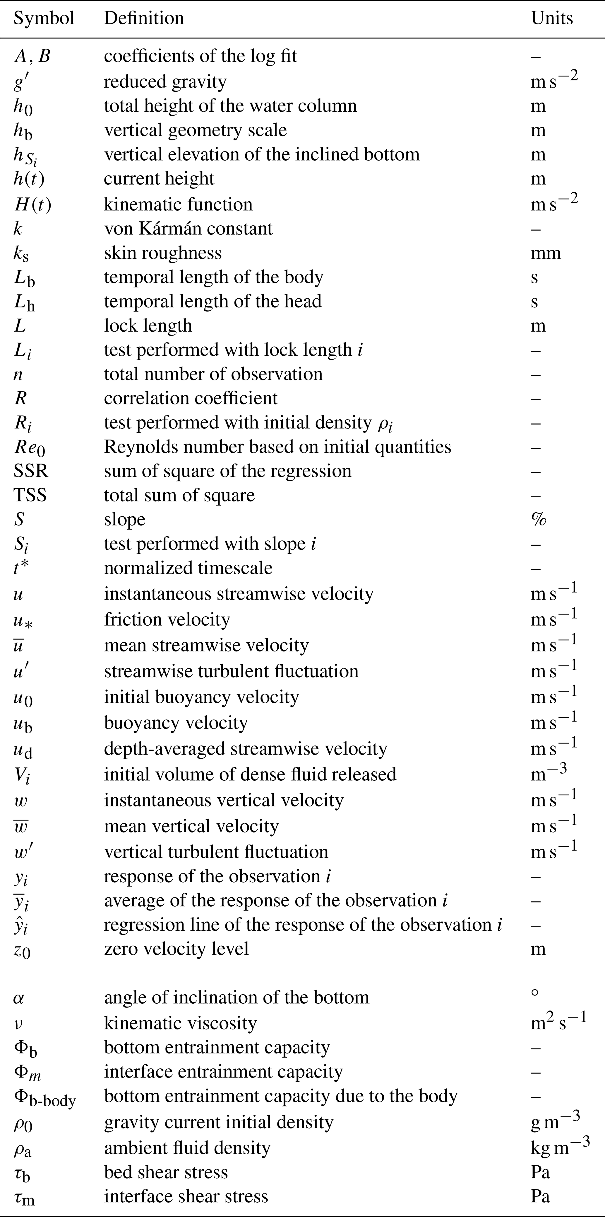
Table A1 summarizes the list of symbols used in the paper, their definition and unit of measure.

Table A1 List of symbols with definition and unit of measure.