An index concentration method for suspended load monitoring in large rivers of the Amazonian foreland

Because increasing climatic variability and anthropic pressures have affected the sediment dynamics of large tropical rivers, long-term sediment concentration series have become crucial for understanding the related socioeconomic and environmental impacts. For operational and cost rationalization purposes, index concentrations are often sampled in the flow and used as a surrogate of the cross-sectional average concentration. However, in large rivers where suspended sands are responsible for vertical concentration gradients, this index method can induce large uncertainties in the matter fluxes.

Assuming that physical laws describing the suspension of grains in turbulent flow are valid for large rivers, a simple formulation is derived to model the ratio (α) between the depth-averaged and index concentrations. The model is validated using an exceptional dataset (1330 water samples, 249 concentration profiles, 88 particle size distributions and 494 discharge measurements) that was collected between 2010 and 2017 in the Amazonian foreland. The α prediction requires the estimation of the Rouse number (P), which summarizes the balance between the suspended particle settling and the turbulent lift, weighted by the ratio of sediment to eddy diffusivity (β). Two particle size groups, fine sediments and sand, were considered to evaluate P. Discrepancies were observed between the evaluated and measured P, which were attributed to biases related to the settling and shear velocities estimations, but also to diffusivity ratios β≠1. An empirical expression taking these biases into account was then formulated to predict accurate estimates of β, then P ($\mathrm{\Delta }P=\pm \mathrm{0.03}$) and finally α.

The proposed model is a powerful tool for optimizing the concentration sampling. It allows for detailed uncertainty analysis on the average concentration derived from an index method. Finally, this model could likely be coupled with remote sensing and hydrological modeling to serve as a step toward the development of an integrated approach for assessing sediment fluxes in poorly monitored basins.

1 Introduction

In recent decades, the Amazon Basin has experienced an intensification in climatic variability (e.g., Gloor et al., 2013; Marengo and Espinoza, 2015), specifically in extreme events (drought and flood), as well as increasing anthropic pressure. In the Peruvian foreland, the advance of the pioneer fronts causes serious changes in land use, which are enhanced by the proliferation of roads that provide access to the natural resources hosted by this region. The number of hydropower projects is also rapidly increasing (e.g., Finer and Jenkins, 2012; Latrubesse et al., 2017; Forsberg et al., 2017). These global and local changes might increase the erosion rates in the basin as well as the suspended load interannual variability (e.g., Walling and Fang, 2003; Martinez et al., 2009). The sediment transfer dynamics might also be affected (e.g., Walling, 2006), generating large ecological impacts on the mega-diverse Amazonian biome and having socioeconomic consequences on the riverine populations. In such a context, long-term and reliable sediment series are crucial for detecting, monitoring and understanding the related socioeconomic and environmental impacts (e.g., Walling, 1983, 2006; Horowitz, 2003; Syvitski et al., 2005; Horowitz et al., 2015). However, there is a lack of consistent data available for this region, and this lack of data has prompted an increased interest in developing better spatiotemporal monitoring of sediment transport.

In the large tropical rivers of Peru, the measurement of cross-sectional average concentrations 〈C〉 (mg L⁻¹) remains a costly and time-consuming task. First, gauging stations can only be reached after several days of traveling on hard dirt roads or by the river. Second, there is no infrastructure on the rivers, and all operations are conducted using small boats under all flow conditions. Third, the gauging sections have depths that range from the metric to the decametric scale and widths that range from the hectometer to the kilometer scale. Such large sections experience pronounced sediment concentration gradients and grain size sorting, in both the vertical and the transverse directions (e.g., Curtis et al., 1979; Vanoni, 1979, 1980; Horowitz and Elrick, 1987; Filizola and Guyot, 2004; Filizola et al., 2010; Bouchez et al., 2011; Lupker et al., 2011; Armijos et al., 2013, 2016; Vauchel et al., 2017). The balance between the local hydrodynamic conditions and the sediment characteristics (e.g., grain size, density and shape) drive this spatial heterogeneity. Thus, the sand suspension is characterized by a high vertical gradient as well as a significant lateral variability, and the concentration varies by several orders of magnitude; in contrast, the fine sediments (e.g., clays and silts) are transported homogeneously throughout the entire river section.

As a consequence, the entire cross section must be explored to provide a representative estimate of the mean concentration of coarse particles. Thus, it is necessary to identify a trade-off between the need to sample an adequate number of verticals and points throughout the cross section and the need for time-integrated or repeated measurements to ensure the temporal representativeness of each water sample (Gitto et al., 2017). The second-order moments of the Navier–Stokes equations induce this temporal concentration variability, as do the larger turbulent structures (typically those induced by the bedforms) and the changes in flow conditions (e.g., backwaters, floods and flow pulses). Sands and coarse silts are much more sensitive to velocity fluctuations than clay particles are (i.e., settling laws are highly sensitive to the diameter of the particles) and are the most difficult to accurately measure.

Depth-integrated or point-integrated sampling procedures are traditionally used to determine the mean concentration of suspended sediment in rivers. However, deploying these methods from a boat is rarely feasible due to the velocity and depth ranges that are encountered in large Amazonian rivers. For a point-integrated bottle sampling method, maintaining a position for a duration long enough to capture a representative water sample (Gitto et al., 2017) requires anchoring the boat and using a heavy ballast. This type of operation is very risky without good infrastructure and well-trained staff, especially when collecting measurements near the river's bottom. Moreover, this method decreases the number of samples that can be collected in 1 d.

For a depth-integrated sampling method within a deep river, the bottle may fill up before reaching the water surface if its transit speed is too slow. Moreover, if the ballast weight is not sufficient to hold the sampler nose in a horizontal position, the filling conditions are not isokinetic, and, therefore, the sample will be nonrepresentative.

Indirect surrogate technologies (e.g., laser diffraction technology or high-frequency acoustic instruments with multi-transducers) may also be used. These instruments provide access to the temporal variability in concentration or grain size; however, they have limited ranges, post-processing complexity (Gray and Gartner, 2010; Armijos et al., 2016) and higher maintenance costs due the fragility of the instruments.

Thus, sampling methods with instantaneous capture or short-term integration (<30 s) are preferred. These methods follow a relevant grid of sample points (Xiaoqing, 2003; Filizola and Guyot, 2004; Bouchez et al., 2011; Armijos et al., 2013; Vauchel et al., 2017). The mean concentration 〈C〉 (mg L⁻¹) is determined by combining all samples into a single representative discharge-weighted concentration value, which is depth-integrated and cross-sectionally representative (Xiaoqing, 2003; Horowitz et al., 2015; Vauchel et al., 2017). In the present study, the spatial distribution of the concentration within the cross section is summarized into a single concentration profile that is assumed to be representative of the suspension regime along the river reach. The water depth h (m) becomes the mean cross-section depth, which is close to the hydraulic radius for large rivers. Therefore, 〈C〉 will be hereafter defined as the depth-integration of this concentration profile C(z), z (m) being the height above the bed, from a reference height z₀ (m) just above the riverbed (z₀≪h) to the free surface, and weighted by the depth-averaged velocity $\langle u\rangle =\frac{\mathrm{1}}{h}{\int }_{z_{\mathrm{0}}}^{h}u\left(z\right)\mathrm{d}z$ (m s⁻¹) (a term list can be found in the appendices):

$$\begin{array}{}\text{(1)}& \langle C\rangle ={\displaystyle \frac{{\int }_{z_{\mathrm{0}}}^{h}C\left(z\right)\times u\left(z\right)\mathrm{d}z}{{\int }_{z_{\mathrm{0}}}^{h}u\left(z\right)\mathrm{d}z}}.\end{array}$$

However, to dampen the random uncertainties mainly related to the coarse sediments, this procedure requires taking a statistically significant number of samples throughout the cross section, which is also time- and labor-intensive.

All of these limitations preclude the application of such complete sampling procedures at a relevant time-step necessary to build up a detailed concentration series. By analogy with the index velocity method for discharge computation (Levesque and Oberg, 2012), derived surrogate procedures, called index sampling methods (Xiaoqing, 2003), are thus preferred. One or a few “index samples” are taken as proxies of 〈C〉, usually at the water surface (e.g., Filizola and Guyot, 2004; Bouchez et al., 2011; Vauchel et al., 2017). The index concentration monitoring frequency is then scheduled to suit the river's hydrological behavior and minimize the random uncertainties on the measured index concentration C(z_χ) (mg L⁻¹) (Duvert et al., 2011; Horowitz et al., 2015).

The index concentration method first requires a robust site-specific calibration between the two concentrations of interest, 〈C〉 and C(z_χ), i.e., for all hydrological conditions, which cannot always be achieved under field conditions. Such relations are usually expressed with the following linear form (e.g., Filizola, 2003; Guyot et al., 2005, 2007; Espinoza-Villar et al., 2012; Vauchel et al., 2017):

$$\begin{array}{}\text{(2)}& \langle C\rangle =\mathit{\alpha }C\left(z_{\mathit{\chi }}\right)+\mathit{\xi },\end{array}$$

where the regression slope α and the intercept ξ are the fitted parameters of the empirical model. In this study, the intercept will be assumed to be zero (ξ=0). The dispersion and the extrapolation of the $\mathit{\alpha }=\langle C\rangle /C\left(z_{\mathit{\chi }}\right)$ may induce substantial uncertainties in the matter fluxes (Vauchel et al., 2017). Most of this uncertainty is attributable to C(z_χ) (Gitto et al., 2017), particularly when only a single index sample is taken or when a unique sample position is considered. Indeed, the relation may change around this position based on the flow conditions.

The index sample representativeness becomes crucial as high-resolution imagery is increasingly used to link remote-sensing reflectance data with the suspended sediment concentration (e.g., Mertes et al., 1993; Martinez et al., 2009, 2015; Espinoza-Villar et al., 2012, 2013, 2017; Park and Latrubesse, 2014; Dos Santos et al., 2017). These advanced techniques finally provide a spatially averaged C(z_χ) value for the finest grain sizes at the water surface of a reach (Pinet et al., 2017), which must be correlated with the total mean concentration transported in the reach of interest (i.e., including the sand fraction when possible) to be a quantitative measurement (Horowitz et al., 2015). Hence, to improve our knowledge of the sediment delivery problem (Walling, 1983), these empirical relations deserve hydraulic-based understanding.

In this study, the ratios $\mathit{\alpha }=\langle C\rangle /C\left(z_{\mathit{\chi }}\right)$ observed at eight gauging stations in the Amazonian foreland were analyzed to identify the main parameters that controlled their variability. Assuming that the shape of the concentration profiles measured in large Amazonian rivers can be well described using a physically based model for sediment suspension, the possibility of deriving a simple formulation for the ratio α using this model was investigated. This assumption is supported by previous studies that specifically showed that the Rouse model (Rouse, 1937) can describe the suspension of sediments in large tropical rivers well (Vanoni, 1979, 1980; Bouchez et al., 2011; Lupker et al., 2011; Armijos et al., 2016). However, the Rouse model predicts a concentration of zero at the water surface, which is where the index concentration is often sampled. To find an alternative, other formulations (Zagustin, 1968; Van Rijn, 1984; Camenen and Larson, 2008) are compared to the data.

Then, the relevance of the derived model in terms of developing a detailed and reliable sediment flux series with an index method is discussed; specifically, the ability to accurately estimate the model parameters is evaluated. Finally, recommendations for the optimized collection of index samples from large Amazonian rivers are inferred from the proposed model.

2 Materials and methods

2.1 Hydrological data acquisition

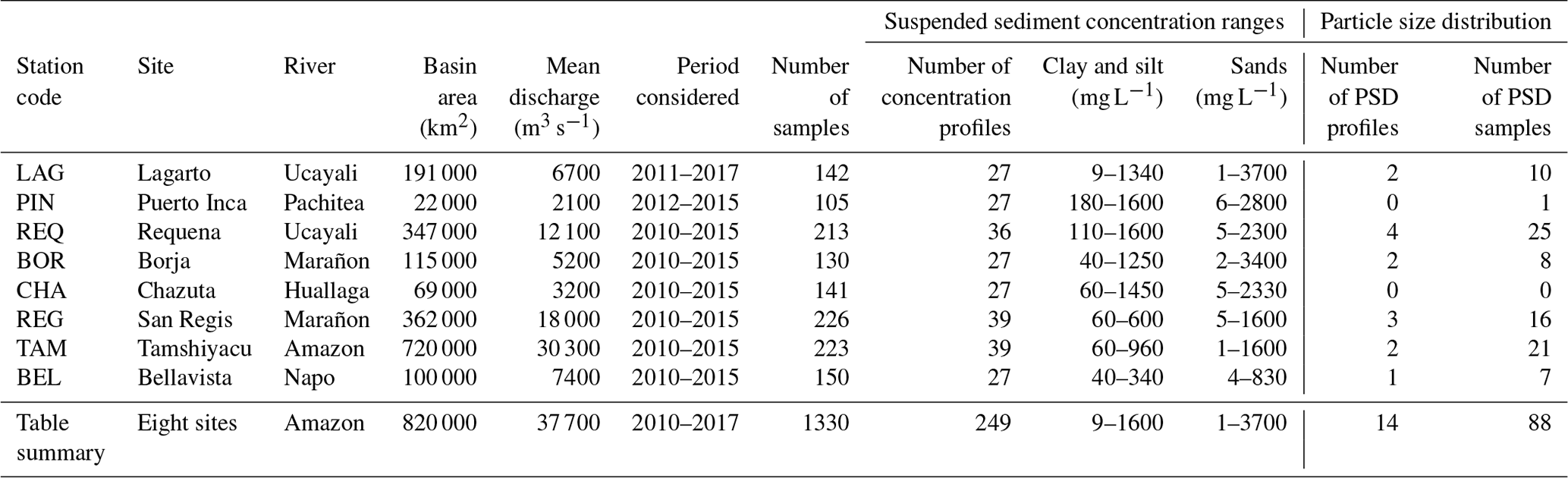
The hydrological data presented here were collected within the international framework of the critical zone observatory HYBAM (HYdrogéochimie du Bassin AMazonien – Geodynamical, hydrological and biogeochemical control of erosion, alteration and material transport in the Amazon Basin), which is a long-term monitoring program. A Franco-Peruvian team, from the IRD (Institut de Recherche pour le Développement) and the SENAMHI (SErvicio NAcional de Meteologia e HIdrologia), operates the eight gauging stations of the HYBAM hydrological network in Peru; of these, four stations control the Andean piedmont fluxes, and four stations control the lowlands (Fig. 1). The three major Peruvian tributaries of the Amazon (Solimões) River, i.e., the Ucayali River, the Marañon River and the Napo River, are monitored. The studied sites cover drainage areas ranging from approximately 22 000 to 720 000 km² and have mean discharges ranging from 2100 to 30 300 m³ s⁻¹ (Table 1). These large tropical rivers have flows with gradually varied conditions, unimodal and diffusive flood waves (except for the Napo River), and subcritical conditions, which enable backwater effects (Dunne et al., 1998; Trigg et al., 2009).

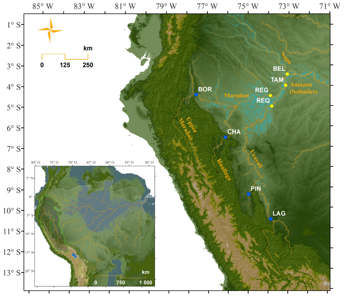
Figure 1 Location of the sampling sites in the Amazon Basin. Blue squares represent piedmont gauging stations, yellow dots represent lowland gauging stations and cyan represents flooded areas.

Table 1 Hydrologic and sample dataset for the eight sampling stations.

The Amazonian foreland in Peru has a humid tropical regime (Guyot et al., 2007; Armijos et al., 2013), and large amounts of runoff are produced during the austral summer. During the austral winter, the maximum continental rainfall is located to the north of the Equator, in line with the intertropical convergence zone (Garreaud et al., 2009). Thus, the numerous water supplies from the Ecuadorian subbasins smooth the seasonality of the Marañon River flow regime. Located further to the south, the Ucayali Basin experiences a pronounced dry season (Ronchail and Gallaire, 2006; Garreaud et al., 2009; Lavado et al., 2011; Santini et al., 2014).

The El Niño–Southern Oscillation (ENSO) might alter these dynamics, as there are severe low-flow events in El Niño years and heavy rainfall events in La Niña years (Aceituno, 1988; Ronchail et al., 2002; Garreaud et al., 2009). These events seriously affect the sediment routing processes (e.g., Aalto et al., 2003), as do other extreme events unrelated to the ENSO (e.g., Molina-Carpio et al., 2017).

2.1.1 Sampling strategy

For the reasons outlined in Sect. 1, local observers monitor surface index concentrations at each station following a hydrology-based scheme. The sampling depth is typically 20–50 cm below the water surface. The samples are taken in the mainstream and at a fixed position. Additionally, HYBAM routinely uses MODIS images to determine surface concentrations, and these values are calibrated with in situ radiometric measurements (Espinoza-Villar et al., 2012; Santini et al., 2014; Martinez et al., 2015).

For calibration purposes (i.e., water level vs. discharge and concentration index vs. mean concentration), 44 campaigns were conducted during the 2010–2017 period. These campaigns included the collection of 494 discharge measurements, 249 sediment concentration profiles and 1330 water samples. The dataset covers contrasted regimes, including periods of extreme droughts (e.g., 2010) and periods of extreme floods (e.g., 2012 and 2015) (Espinoza et al., 2012, 2013; Marengo and Espinoza, 2015). Thus, the sampled concentrations spanned a wide range (Table 1), which represented the river hydrological variability well. A 600 kHz Teledyne RDI Workhorse acoustic Doppler current profiler (ADCP) was used and coupled with a 5 Hz GPS sensor to correct for the movable bed error (e.g., Callède et al., 2000; Vauchel et al., 2017).

A point sampling method was preferred to estimate 〈C〉 (Filizola, 2003; Guyot et al., 2005; Vauchel et al., 2017) to capture the vertical concentration distribution. The sampling for concentration determination was usually performed at the following height (h) from the bed: ∼0.98h, 0.75h, 0.5h, 0.25h, sometimes at ∼0.15h and finally at ∼0.1h, at three verticals that divided the cross section according to the river width or the flow rate. Each vertical was assumed to be representative of the flow in the corresponding subsection. Sampling was performed from a boat drifting on a streamline immediately after the ADCP measurements were collected. The sampler capacity was 650 mL, with a filling time of ∼10 s, which allowed for a short time integration along the streamline passing by the sample point. Considering the waves at the free surface, the boat's pitch and roll and the bedforms, the accuracy of the vertical position of the sampler may be evaluated as ±0.5 m. This variability leads to substantial uncertainty in the zones with high concentration gradients. The operation time was approximately 2–5 h, depending on the river sites. Steady conditions were observed during the sampling operation.

Finally, samples for the characterization of the bed material PSD were collected at four sites: BEL, REQ, REG and TAM. The bed material was dragged on the riverbed.

2.1.2 Analytical methods

The concentrations C_ϕ for two main grain size fractions ϕ were further determined: the sand fraction (ϕ=s) was separated from the silt/clay fraction (ϕ=f) using a 63 µm sieve (cf. Standart Methods ASTM D3977), according to the Wentworth (1922) grain size classification for noncohesive particles. The water samples were filtered using 0.45 µm cellulose acetate filters (Millipore) that were then dried at 50 ^∘C for 24 h.

Particle size analysis was performed with a Horiba LA-920-V2 laser diffraction sizer. The entire sampled volume was analyzed, with several repetitions demonstrating excellent analytical reproducibility. For each size group ϕ, the arithmetic mean diameter d_ϕ (m) was calculated:

$$\begin{array}{}\text{(3)}& d_{\mathit{\varphi }}={\displaystyle \frac{{\sum }_i{d}_i{X}_i}{{\sum }_i{X}_i}},\end{array}$$

where X_i is the relative content in the PSD for the class of diameter d_ϕ. The settling velocities w_ϕ corresponding to the diameters d_ϕ derived from the PSD were computed using the Soulsby (1997) law, which assumed a particle density of 2.65 g cm⁻³.

2.2 Theory for modeling vertical concentration profiles

Schmidt (1925) and O'Brien (1933) proposed a diffusion–convection equation to model the time-averaged vertical concentration distribution C_ϕ(z) of grains settling with a velocity w_ϕ (m s⁻¹). The grain size, shape and density are considered to be uniform. The equation is expressed as follows:

$$\begin{array}{}\text{(4)}& {\mathit{\epsilon }}_{\mathit{\varphi }}{\displaystyle \frac{\partial C_{\mathit{\varphi }}}{\partial z}}=-w_{\mathit{\varphi }}{C}_{\mathit{\varphi }},\end{array}$$

where the term on the left side is the rate of upward concentration diffusion caused by turbulent mixing, balanced by the settling mass flux in the right term. ε_ϕ (m² s⁻¹) is the sediment diffusivity coefficient that characterizes the particle exchange capacity for two eddies positioned on both sides of a horizontal fictitious plane. ε_ϕ is assumed to be proportional to the momentum exchange coefficient ε_m (m² s⁻¹) (Rouse, 1937):

$$\begin{array}{}\text{(5)}& {\displaystyle \frac{{\mathit{\epsilon }}_{\mathit{\varphi }}}{{\mathit{\epsilon }}_{\mathrm{m}}}}={\mathit{\beta }}_{\mathit{\varphi }},\end{array}$$

where the β_ϕ parameter is similar to the inverse of a turbulent Schmidt number (Graf and Cellino, 2002; Camenen and Larson, 2008). It may be depth-averaged (Van Rijn, 1984) or considered to be independent of the height above the bed (Rose and Thorne, 2001).

The main issue of the Schmidt–O'Brien formulation (Eq. 4) is the expression of the vertical distribution of the sediment mass diffusivity ε_ϕ. Once this term is modeled (models are given in the following), Eq. (4) is depth-integrated from the reference height z₀ to the free surface to obtain the expression of the concentration distribution along the water column. The concentration C_ϕ(z₀) is then required to determine the magnitude of the profile and can be evaluated using a bed-load transport equation (e.g., Van Rijn, 1984; Camenen and Larson, 2008) or measured directly. However, in the case of a sampling operation, the large concentration gradient observed near the riverbed would force the operator to sample water at the reference height z₀ with a very high precision to minimize uncertainties; however, achieving such a high level of precision is rarely possible. Hence, it is preferable to choose a more reliable reference concentration in the interval $z=[z_{\mathrm{0}},h]$. Thus, the following formulae resulting from Eq. (4) are written using C_ϕ(z_χ) instead of C_ϕ(z₀) as a reference.

Building on Prandtl's concept of mixing length distribution, O'Brien (1933) and Rouse (1937) expressed the sediment diffusion profile using the following parabolic form:

$$\begin{array}{}\text{(6)}& {\mathit{\epsilon }}_{\mathit{\varphi }}\left(z\right)={\mathit{\beta }}_{\mathit{\varphi }}\mathit{\kappa }{u}_{\ast }z\left(\mathrm{1}-{\displaystyle \frac{z}{h}}\right),\end{array}$$

where κ is the Von Kármán constant, and u_∗ (m s⁻¹) is the shear velocity. This expression leads to the classic Rouse equation (Rouse, 1937) for suspended concentration profiles. For $z_{\mathit{\chi }}\in \left[z_{\mathrm{0}},h\right[$:

$$\begin{array}{}\text{(7)}& {\displaystyle \frac{C_{\mathit{\varphi }}\left(z\right)}{C_{\mathit{\varphi }}\left(z_{\mathit{\chi }}\right)}}={\left({\displaystyle \frac{z_{\mathit{\chi }}}{z}}\times {\displaystyle \frac{h-z}{h-z_{\mathit{\chi }}}}\right)}^{P_{\mathit{\varphi }}},\end{array}$$

where $P_{\mathit{\varphi }}=w_{\mathit{\varphi }}/{\mathit{\beta }}_{\mathit{\varphi }}\mathit{\kappa }{u}_{\ast }$ is the Rouse suspension parameter, i.e., the ratio between the upward turbulence forces and the downward gravity forces. P_ϕ is the shape factor for the concentration profile. The Rouse formulation is widely used in open channels and suits the observed profiles in the Amazon River well (Vanoni, 1979, 1980; Bouchez et al., 2011; Armijos et al., 2016). However, the Rouse formulation predicts a concentration of zero at the water surface. Three other simple models, for which C_ϕ(h)≠0, have been selected in this work to overcome this problem, i.e., the Zagustin (1968), Van Rijn (1984) and Camenen and Larson (2008) models.

Zagustin (1968) proposed a formulation for the eddy diffusivity distribution based on experimental measurements and a defect law for the velocity distribution. The following variable changes were introduced: $Z=\sqrt{(h-z)/z}$, and the sediment diffusivity formulation proposed by Zagustin (1968) is

$$\begin{array}{}\text{(8)}& {\mathit{\epsilon }}_{\mathit{\varphi }}\left(Z\right)={\mathit{\beta }}_{\mathit{\varphi }}{\displaystyle \frac{\mathit{\kappa }}{\mathrm{3}}}{u}_{\ast }hZ{\left(\mathrm{1}-Z^{\mathrm{2}}\right)}^{\mathrm{3}}.\end{array}$$

This leads to an expression with a finite value at the water surface:

$$\begin{array}{}\text{(9)}& \left\{\begin{array}{l}{\displaystyle \frac{C_{\mathit{\varphi }}\left(z\right)}{C_{\mathit{\varphi }}\left(z_{\mathit{\chi }}\right)}}=\exp \left(P_{\mathit{\varphi }}\left(\mathrm{\Phi }\left(z_{\mathit{\chi }}\right)-\mathrm{\Phi }\left(z\right)\right)\right)\\ \mathrm{\Phi }={\displaystyle \frac{\mathrm{1}}{\mathrm{2}}}\ln \left({\displaystyle \frac{\left(Z^{\mathrm{3}}+\mathrm{1}\right){\left(Z-\mathrm{1}\right)}^{\mathrm{3}}}{\left(Z^{\mathrm{3}}-\mathrm{1}\right){\left(Z+\mathrm{1}\right)}^{\mathrm{3}}}}\right)+\sqrt{\mathrm{3}}\arctan \left({\displaystyle \frac{\sqrt{\mathrm{3}}Z}{Z^{\mathrm{2}}-\mathrm{1}}}\right)\end{array}\right..\end{array}$$

As the proposed diffusivity profile is slightly different from the parabolic form, this expression leads to P_ϕ values that are approximately 7 % lower than those obtained with the Rouse theory (Zagustin, 1968).

Van Rijn (1984) proposed a parabolic-constant distribution for sediment diffusivity, i.e., a parabolic profile in the lower half of the flow depth (Eq. 6) and a constant value in the upper half of the flow depth (Eq. 10), which corresponds to the maximum diffusivity predicted by the Prandtl–Von Kármán theories. Indeed, some authors have reported measurements with constant sediment diffusivity in the upper layers (Coleman, 1970; Rose and Thorne, 2001).

$$\begin{array}{}\text{(10)}& {\mathit{\epsilon }}_{\mathit{\varphi }}\left(z\ge \mathrm{0.5}h\right)={\displaystyle \frac{{\mathit{\beta }}_{\mathit{\varphi }}}{\mathrm{4}}}\mathit{\kappa }{u}_{\ast }h.\end{array}$$

Therefore, for z≥0.5h, the concentration profile is exponential, with a finite value at the free surface:

$$\begin{array}{}\text{(11)}& {\displaystyle \frac{C_{\mathit{\varphi }}\left(z\right)}{C_{\mathit{\varphi }}\left(z_{\mathit{\chi }}\right)}}={\left({\displaystyle \frac{z_{\mathit{\chi }}}{h-z_{\mathit{\chi }}}}\right)}^{P_{\mathit{\varphi }}}\exp \left(-\mathrm{4}P\left({\displaystyle \frac{z}{h}}-{\displaystyle \frac{\mathrm{1}}{\mathrm{2}}}\right)\right).\end{array}$$

In addition, Van Rijn (1984) introduced a coefficient to account for the dampening of the fluid turbulence by the sediment particles. This coefficient value is equal to the unity if the sediment diffusion ε_ϕ distribution is concentration-independent, which was an assumption used in the present work because of the range of concentrations measured in the Amazonian lowland rivers (Table 1), and discussed further in Sect. 4.1.

Camenen and Larson (2008) showed that the depth-averaged sediment diffusivity ${\mathit{\epsilon }}_{\mathit{\varphi }}=\frac{{\mathit{\beta }}_{\mathit{\varphi }}}{\mathrm{6}}\mathit{\kappa }{u}_{\ast }h$ is a reasonable approximation of the Prandtl–Von Kármán parabolic form (Eq. 10) that does not significantly affect the prediction of the concentration profiles in large rivers (P_ϕ<1), except near the boundaries. This simple expression for ε_ϕ lead to an exponential sediment concentration profile:

$$\begin{array}{}\text{(12)}& {\displaystyle \frac{C_{\mathit{\varphi }}\left(z\right)}{C_{\mathit{\varphi }}\left(z_{\mathit{\chi }}\right)}}=\exp \left({\displaystyle \frac{\mathrm{6}{P}_{\mathit{\varphi }}}{h}}\left(z_{\mathit{\chi }}-z\right)\right).\end{array}$$

This profile has practical interest: there is no need to define the reference level z₀ accurately or estimate the corresponding concentration C₀ (Camenen and Larson, 2008).

2.3 A general expression for the ratio α

2.3.1 Assumptions and formalism

C_ϕ(z) can be expressed by each of the models presented in this section (Eqs. 7, 9, 12) and substituted into Eq. (1) to calculate 〈C_ϕ〉. Then, the development of the expression ${\mathit{\alpha }}_{\mathit{\varphi }}=\langle C_{\mathit{\varphi }}\rangle /C_{\mathit{\varphi }}\left(z_{\mathit{\chi }}\right)$ would lead to the following equation, which is similar to Eq. (2), where the parameters driving α_ϕ are identified:

$$\begin{array}{}\text{(13)}& {\displaystyle \frac{\langle C_{\mathit{\varphi }}\rangle }{C_{\mathit{\varphi }}\left(z_{\mathit{\chi }}\right)}}={\mathit{\alpha }}_{\mathit{\varphi }}\left({\displaystyle \frac{z_{\mathrm{0}}}{h}},{\displaystyle \frac{z_{\mathit{\chi }}}{h}},P_{\mathit{\varphi }},u\right).\end{array}$$

However, the PSDs observed in large rivers are rather broad (e.g., Bouchez et al., 2011; Lupker et al., 2011; Armijos et al., 2016) and may be binned in a range of n grain size fractions ϕ, as modeling the concentration profiles requires the diameter of sediment in suspension d_ϕ to be almost constant throughout the water depth if there is not a narrow PSD. Assuming that the interaction between sediment classes ϕ is negligible, it is possible to apply Eq. (7) and use a multiclass configuration to describe the PSD:

$$\begin{array}{}\text{(14)}& \mathit{\alpha }=\sum _{\mathit{\varphi }=\mathrm{1}}^n{\mathit{\alpha }}_{\mathit{\varphi }}{X}_{\mathit{\varphi }},\end{array}$$

where X_ϕ is the mass fraction of each grain size fraction measured for the index sample with the concentration C_ϕ(z_χ) ($\sum _{i=\mathrm{1}}^n{X}_{\mathit{\varphi }}=\mathrm{1}$). Moreover, it can be shown that the weight of the velocity distribution on the depth-averaged concentration may be neglected in Eq. (1) when the suspension occurs throughout the water column, i.e., when P_ϕ<0.6 . Thus, if P_ϕ<0.6, it is possible to express ${\mathit{\alpha }}_{\mathit{\varphi }}\left(z_{\mathrm{0}}/h,z_{\mathit{\chi }}/h,P_{\mathit{\varphi }}\right)$.

A key issue is then to provide a proper model of the PSD using a limited number of sediment classes. In this study, the available dataset provides concentrations for fine particles ($\mathrm{0.45}<d_{\mathrm{f}}<\mathrm{63}$ µm) and sand particles (d_s≥63 µm). Then, the ratio α may be formalized as follows:

$$\begin{array}{}\text{(15)}& \mathit{\alpha }=X_{\mathrm{f}}{\mathit{\alpha }}_{\mathrm{f}}+X_{\mathrm{s}}{\mathit{\alpha }}_{\mathrm{s}}.\end{array}$$

Thus, if at height z_χ the mass fraction of each group is accurately known after sieving, α may be calculated for the whole PSD.

2.3.2 Model proposed for the ratio α_ϕ prediction in Amazonian large rivers

The depth-integration of the Camenen and Larson formulation (Eq. 12) is considered to be a reasonable approximation of the measured 〈C〉 in large rivers (Camenen and Larson, 2008), with a simple expression that is independent of the z₀ term, which differs from the other theories presented above. Moreover, in the next section, the fit of the suspension models to the measured concentration profiles will show that the Zagustin model provides the best fit to the observations, particularly in the upper layer of the flow. Thus, in this work, C_ϕ(z_χ) will be expressed using the Zagustin model (Eq. 9), and 〈C〉 will be expressed using the Camenen and Larson model.

Because the Zagustin model causes the Rouse number ($P_{\mathit{\varphi }}^{\prime }$) to be slightly smaller than that calculated with the Rouse model ($P_{\mathit{\varphi }}^{\prime }\approx \mathrm{0.93}{P}_{\mathit{\varphi }}$, according to Zagustin, 1968), we obtain the following expression for predicting the ratio α_ϕ:

$$\begin{array}{}\text{(16)}& {\mathit{\alpha }}_{\mathit{\varphi }}(z_{\mathit{\chi }},P_{\mathit{\varphi }})={\displaystyle \frac{\exp \left(\mathrm{6}{P}_{\mathit{\varphi }}\frac{z_{\mathrm{r}}}{h}\right)\left(\mathrm{1}-\exp \left(-\mathrm{6}{P}_{\mathit{\varphi }}\right)\right)}{\mathrm{6}{P}_{\mathit{\varphi }}\exp \left(\mathrm{0.93}{P}_{\mathit{\varphi }}\left(\mathrm{\Phi }\left(z_{\mathrm{r}}\right)-\mathrm{\Phi }\left(z_{\mathit{\chi }}\right)\right)\right)}},\end{array}$$

where z_r is a reference height required for expressing C_ϕ(z_χ) with the Zagustin model (z_r replaces z_χ in Eq. 9). Taking z_r=0.5h, the previous expression is simplified:

$$\begin{array}{}\text{(17)}& {\mathit{\alpha }}_{\mathit{\varphi }}(z_{\mathit{\chi }},P_{\mathit{\varphi }})={\displaystyle \frac{\exp \left(\mathrm{3}{P}_{\mathit{\varphi }}\right)\left(\mathrm{1}-\exp \left(-\mathrm{6}{P}_{\mathit{\varphi }}\right)\right)}{\mathrm{6}{P}_{\mathit{\varphi }}\exp \left(\mathrm{0.93}{P}_{\mathit{\varphi }}\left(\mathrm{\Phi }\left(\frac{h}{\mathrm{2}}\right)-\mathrm{\Phi }\left(z_{\mathit{\chi }}\right)\right)\right)}}.\end{array}$$

Nevertheless, other formulations might be inferred from the suspension models. For instance, the Camenen and Larson formulation could be alternatively used to model C_ϕ(z_χ) in the central region of the flow [0.2h,0.8h], which leads to a simpler expression:

$$\begin{array}{}\text{(18)}& {\mathit{\alpha }}_{\mathit{\varphi }}(z_{\mathit{\chi }},P_{\mathit{\varphi }})={\displaystyle \frac{\mathrm{1}}{\mathrm{6}{P}_{\mathit{\varphi }}}}\exp \left(\mathrm{6}{P}_{\mathit{\varphi }}{\displaystyle \frac{z_{\mathit{\chi }}}{h}}\right)\left(\mathrm{1}-\exp \left(-\mathrm{6}{P}_{\mathit{\varphi }}\right)\right).\end{array}$$

2.4 Model fitting strategy

To obtain a reach-scale profile, the fit to the concentrations averaged at each normalized depth z∕h was assessed. It was assumed that the energy gradient, the mean bed roughness factor and the mean diameter did not significantly change from one subsection to another, even if the point-to-point variability was high (Yen, 2002). Thus, the depth becomes the main factor influencing the P_ϕ in the transverse direction. In the cross sections studied here, the variation in depth from one vertical to the next was not sufficient to significantly influence the Rouse number. C_ϕ(z_χ) is then the average of several representative samples taken across the river width at the same relative height (z_χ∕h).

After the first data cleaning of the sampled points, a robust and iteratively re-weighted least squares regression technique was used to minimize the influence of the outlier values. The weight values (W) between z₀ and h were assigned with the following parabolic function, similar to the eddy diffusivity expression (Eq. 6): $W\left(z\right)=z(\mathrm{1}-z)$. Thus, the half-depth point, where the mixing term is the highest, has the largest influence.

Based on the ADCP velocity profile measurements, the parameter z₀ was fixed at $z_{\mathrm{0}}={\mathrm{10}}^{-\mathrm{3}}h$. Indeed, when $z_{\mathrm{0}}<{\mathrm{10}}^{-\mathrm{2}}h$, 〈C〉 is no longer sensitive to z₀ (Eq. 1), even if the Rouse number is not accurately known (Van Rijn, 1984). Hence, $(h-z_{\mathrm{0}})/(z-z_{\mathrm{0}})\approx z/h$ can be assumed when considering reach-scale flow conditions.

2.5 Shear velocity estimation from ADCP transects

The velocity transects measured with an acoustic Doppler current profiler (ADCP) were used to estimate the shear velocities u_∗ from the vertical velocity gradient through the fit of the logarithmic inner law (e.g., Sime et al., 2007; Gualtieri et al., 2018). An average of 30 ADCP “ensembles” (i.e., measurement verticals of velocity), corresponding to about 40 to 70 m in the cross-sectional direction, were required to obtain robust u_∗ values. This was consistent with the methodology applied by Armijos et al. (2016) (50–60 ensembles, corresponding to 10 % of the total width of the section) or Lupker et al. (2011) (30 ensembles, 40 to 70 m). Following these findings, the velocity profiles were averaged over a spanwise length of about 60 m around each concentration profile position. Then, an average of the fitted shear velocities was calculated for each ADCP measurement. The flow over the first 30 m from the riverbanks has been neglected, given the low velocities and the depths in this small area of the cross section.

Furthermore, the imprecise knowledge of the exact bed elevation, the side lobe interferences, the beam angle (which induces a large measurement area), and the instrument's pitch and roll all cause the ADCP velocity data to be inaccurate in the inner flow region (i.e., the region of the flow under bed influence $\sim \left[z_{\mathrm{0}},\mathrm{0.2}h\right]$). However, a fit over the entire height of the measured velocity (∼0.06h to the ADCP “blanking depth” plus the transducer depth) leads to more robust shear velocity values. For that reason, the shear velocities were assessed in the zone between 0.1h and 0.85h.

3 Results

3.1 Data analysis

3.1.1 Index concentration relations calibrated for surface index samples

The observed α ratios for total concentration (i.e., concentration including fine particles and sands) were calculated for a surface index using each field measurement carried out (Fig. 2). Empirical relationships for estimating the total mean concentration from the surface index samples (Eq. 2) were calibrated using these data . The α ratios observed at the three stations monitoring the Ucayali Basin fluxes (i.e., LAG, PIN, and REQ) are similar ($\mathrm{1.3}<\mathit{\alpha }<\mathrm{1.5}$) (Fig. 2). At BEL (Napo River), the α values observed are higher (α≅1.7). Conversely, different trends with larger scatter are observed in the Marañon Basin. The α ratios observed at REG (α≅2.3) are higher than those at BOR (α≅1.5) and CHA (α≅1.4), which are similar to those at LAG, PIN and REQ (Ucayali Basin). However, the observed α values at BOR fluctuate between two main trends, which are represented by the CHA–LAG–PIN–REQ group and the BEL–REG group. At TAM, similarly, the α values rather follow the REG trend at low concentrations before evolving between the REQ and REG trends.

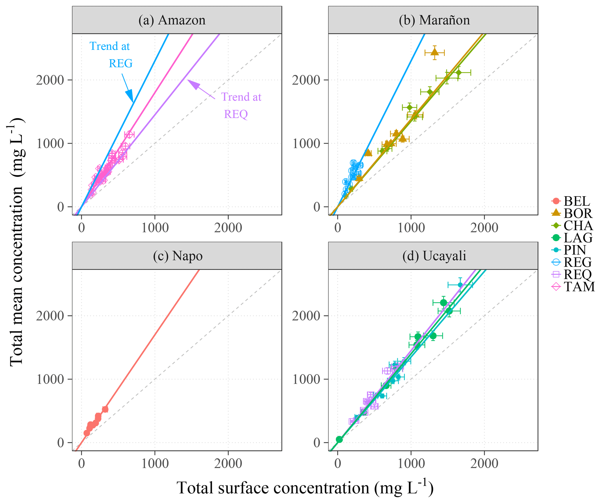
Figure 2 Observed ratios $\mathit{\alpha }=\langle C\rangle /C\left(h\right)$ of the total mean concentration to the total surface concentration, stacked by river basin, with trend lines. For the Amazon River basin at TAM (a), the REG and REQ trend lines were reported. Dashed lines denote the first bisector.

This variability suggests that the α ratio is site-dependent and potentially variable with the flow conditions. It could reflect differences in the basin characteristics (e.g., lithology and climate spatial distributions), then in sediment sources (e.g., mineralogy and PSD) and could relate to the sediment routing in the lowland. The first group (CHA–LAG–PIN–REQ) could be representative of a same source of sediments (the Central Andes), as few lateral inputs come swelling these rivers discharges in the lowland (Guyot et al., 2007; Armijos et al., 2013; Santini et al., 2014). Conversely, in the Marañon lowland, the Ecuadorian tributaries supply almost 55 % of the water discharge and could significantly contribute to the river sediment load. The Napo River example (Laraque et al., 2009; Armijos et al., 2013) shows that the lowland part of the basin can be the main sediment source for these Ecuadorian tributaries. The river incision of this secondary source, and/or the Ecuadorian Andes, could provide coarser elements than the central Andean source does and explain why the ratios α are higher at BEL and REG than at the other sites.

The concentration dataset highlights the control of the sand mass fraction X_s on the ratio α (Fig. 3): α increases with X_s. If finest particles of the PSD are dominant in the index concentrations C_χ sampled in the upper layers of the flow, this wash load is supply-limited, depending on the matter availability, rainfall upon the sources and sediment entrainment processes occurring on the weathered hillslopes. Wash load is then routed through the foreland without important mass fluctuations (e.g., Yuill and Gasparini, 2011). Significant exchanges between the floodplain and main channel lead to some dilution but also to some remobilization of the huge floodplain sediment stocks of the coarser elements that were previously deposited (e.g., clay aggregates, silts and fine sands). Conversely, the sand transport regime is capacity-limited, depending only on the available energy to route the sediments. As the flow energy significantly decreases with the decreasing bed slope, the sand suspended load is gradually decoupled from the wash load in the floodplain, and the wash-load concentration is no longer a good proxy of the coarse particle concentration. The floodplain incision mechanically increases the sand mass fraction X_s in the suspended load. Implicitly, the PSD mean diameter shifts with X_s, but it does not mean that there is any change in the physical properties (e.g., diameter, density and shape) of the sand fraction. This shift directly affects α, as the vertical concentration gradient depends on the balance between the turbulence strength and the settling velocity (Eq. 4). This result highlights the key challenge of providing a proper model of the PSD using a limited number of sediment classes, and validates the discrete approach proposed to model α.

Figure 3 Observed ratios $\mathit{\alpha }=\langle C\rangle /C\left(h\right)$ of the total mean concentration to the total index concentration sampled at the water surface vs. the sand mass fraction X_s.

3.1.2 Particle size profiles

The measured particle size distributions (PSDs) show a multimodal pattern (Fig. 4a). This example of a global PSD that includes the entire particle size range was deconvoluted, assuming a mixture of lognormal subdistributions (e.g., Masson et al., 2018). On the left side of the PSD, a weak lognormal mode was detected in the clay range, but it was negligible in comparison to the silt volume. A fairly uniform fraction of fine sands (d_s≅80 µm) that were transported in suspension throughout the water column with a nearly constant mode over depth was identified. This fraction approximately corresponds to the diameters less than the 10th percentile of the riverbed PSD. A second sand class (d_s≅200 µm) is transported as graded suspension with a strong vertical gradient limited to the lower part of the water column ($z/h<\mathrm{0.2}$). The Rouse number P_ϕ varies from one to six for this class of sediments, suggesting that bed load may be non-negligible. However, the concentration dataset does not contain any bed-load sample close enough to the riverbed and taken with a relevant integration time to assess this argument.

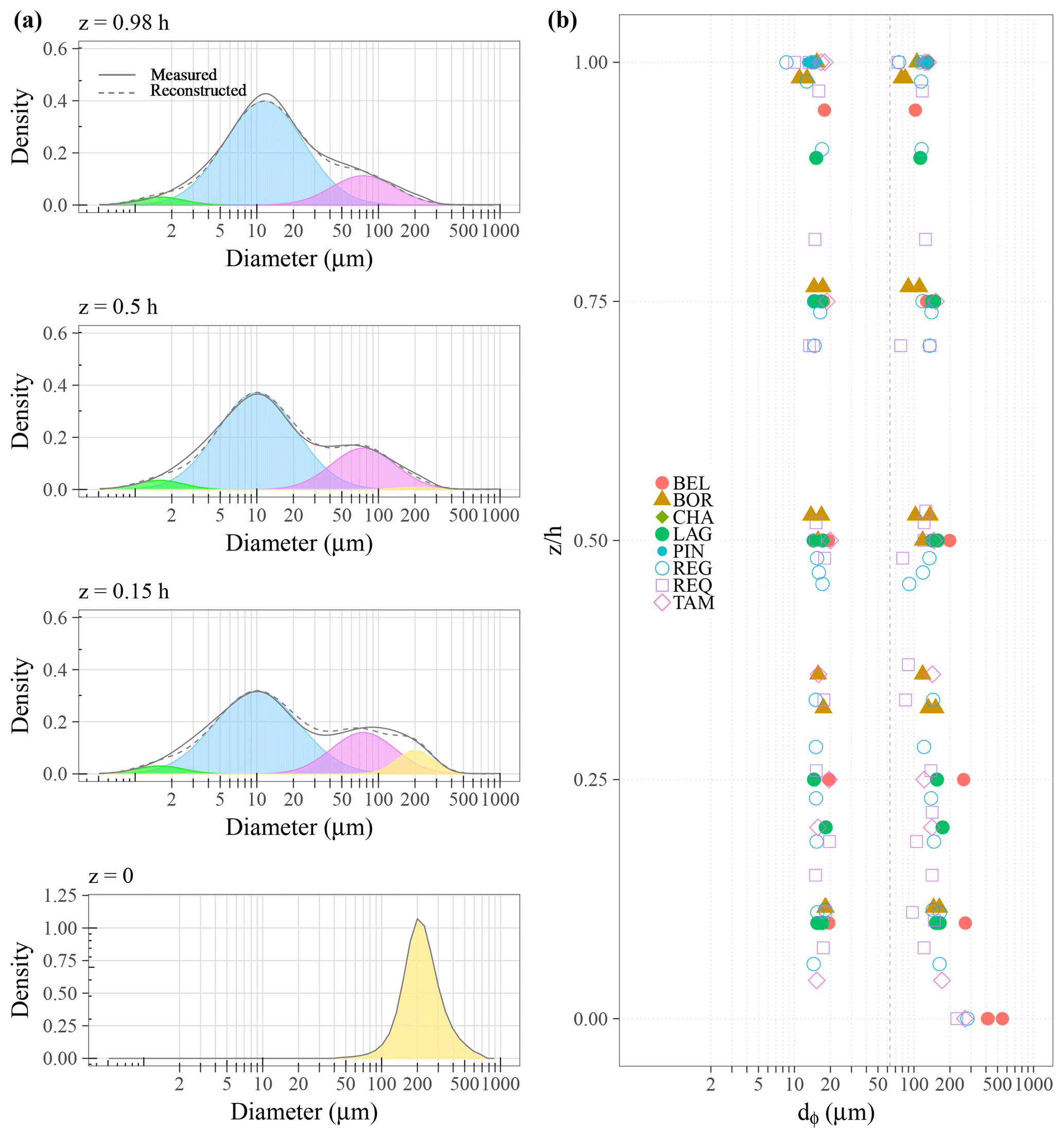
Figure 4 (a) Multimodal modeling of a typical PSD vertical profile. Gray lines represent the PSD measured at the Requena gauge station (16 March 2015) on the Ucayali River. Sampling depths are mentioned on top of each panel. Green, blue, pink and yellow roughly correspond to the following particle size groups: clays, silts and flocculi, very fine sands–fine sands, and bed material, respectively. The dashed gray line is the sum of the subdistributions. (b) Particle diameters d_ϕ measured at the eight sampling stations for the fine and sand fractions.

Concerning the whole dataset of fine sediment mean diameters d_f (Fig. 4b), no vertical gradient was observed for fine sediments, indicating that there was homogeneous mixing throughout the water column, except near the air–water interface, where the calculated d_f tended to decrease. In contrast, a gradient was observed for the sand fraction. Indeed, d_s varied from approximately 300 to 500 µm near the bottom to 80 to 100 µm near the surface. The increased sand diameters d_s in the bottom 0.2h of the water column may be explained by bed material inputs (see the yellow distribution in Fig. 4a).

Nevertheless, modeling the PSD with two size groups, which were characterized by a diameter d_ϕ that was almost constant throughout the water column, was reasonably suitable for the observed PSD, although two more classes (i.e., clay and bed material) could be considered to improve this model. Thus, an average of the diameters derived from the PSD was calculated to summarize the PSD data into one single mean diameter d_ϕ (m) per site for each size group ϕ.

3.2 Suspension model suitability with the measured profiles

The suspension models (Eqs. 7, 9, 11, 12) were fitted to the concentration data to evaluate their suitability to the observed profiles. The dataset confirmed that the Zagustin model causes the Rouse number ($P_{\mathit{\varphi }}^{\prime }$) to be slightly smaller than that calculated using the Rouse model: $P_{\mathit{\varphi }}^{\prime }\approx \mathrm{0.93}{P}_{\mathit{\varphi }}$. The fitted P_ϕ values showed low variability and were summarized by single average values per site, as shown in Table 2. This low variability indicates that there is a dynamic equilibrium between the settling velocity w_ϕ(d_ϕ) and the shear velocity u_∗ under nominal flow conditions, although some extreme values (P_ϕ>0.5) were measured during severe drought events at the lowland stations.

Table 2 Summary of suspended sediment transport parameters for each site and size group.

The Rouse numbers obtained for the fine fraction reflect a suspension regime that is close to the ideal wash load (P_f<0.1, $\mathrm{1}\le {\mathit{\alpha }}_{\mathrm{f}}(h,P_{\mathrm{f}})\le \mathrm{1.5}$). Additionally, regarding the Rouse numbers corresponding to the sand fraction, they reflect a well-developed suspension in the entire water column for the piedmont station group ($\mathrm{0.2}<P_{\mathrm{s}}<\mathrm{0.3}$) and for the lowland station group ($\mathrm{0.35}<P_{\mathrm{s}}<\mathrm{0.45}$), with a significant concentration gradient ($\mathrm{2.3}\le {\mathit{\alpha }}_{\mathrm{s}}(h,P_{\mathrm{s}})\le \mathrm{7.5}$).

Due to the availability, for a given site, of a single mean value of w_ϕ(d_ϕ) per size group, only the corresponding mean values of the diffusivity ratio ${\mathit{\beta }}_{\mathit{\varphi }}=w_{\mathit{\varphi }}/P_{\mathit{\varphi }}\mathit{\kappa }{u}_{\ast }$ were calculated, considering the mean shear velocities (Table 2).

3.2.1 Sediment diffusivity profiles

The diffusivity profiles ε_ϕ(z) were derived from the measured concentration profiles using the discrete form of Eq. (4). In order to capture the small variations in ε_ϕ, accurate sampling is key: the calculation of ε_ϕ requires precise concentration and sampling height values, particularly for the fine fraction, which experiences low vertical concentration gradients.

Nevertheless, the overall shapes of the derived ε_ϕ(z) profiles were in good agreement with the Rouse and Zagustin theories and were slightly closer to the latter (Fig. 5). Given the high scatter of the diffusivity values, Camenen and Larson's expression of depth-averaged diffusivity is a reasonable approximation, except near the bottom and top edges of the diffusivity profiles, where the data departs gradually from this model. However, the constant diffusivity value suggested by Van Rijn (1984) for the upper half of the water column clearly overestimates the diffusivity for z>0.75h. The diffusivity around z=0.75h is, however, overestimated by all the models. The low concentrations near the water surface could result in an underestimation of the ε_ϕ(z≈0.75h) values calculated from the difference $\mathrm{\Delta }{C}_{\mathit{\varphi }}=C_{\mathit{\varphi }}\left(z\approx \mathrm{0.5}h\right)-C_{\mathit{\varphi }}\left(z\approx h\right)$ (Eq. 4). Thus, detailed measurements are required in the upper layer of the flow to confirm the shapes of the ε_ϕ(z) profiles in this zone where the air–water interface and the secondary currents can influence the turbulent mixing profiles.

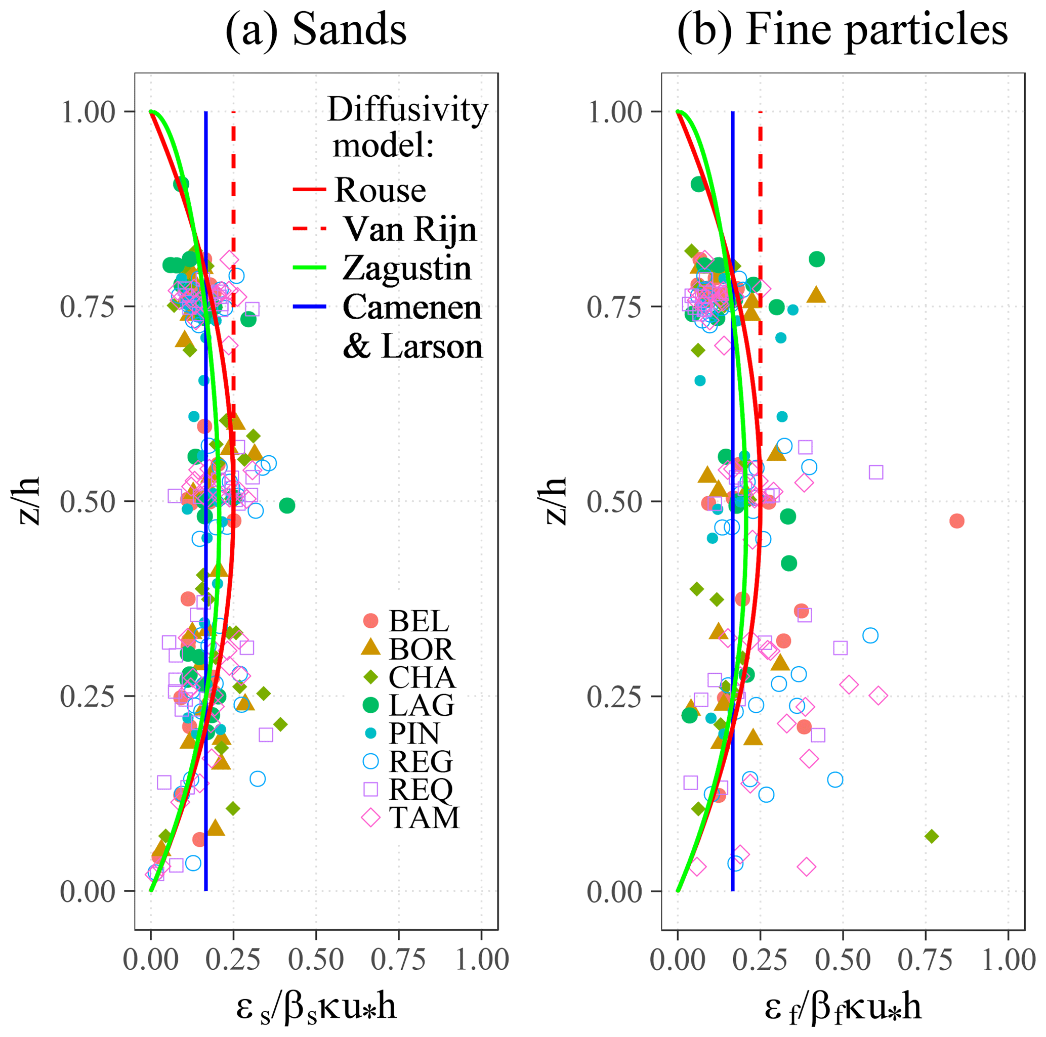
Figure 5 Dimensionless sediment diffusivity coefficient derived from the measured concentration profiles.

3.2.2 Concentration profile suitability

Overall, the suspension models (Eqs. 7, 9, 11, 12) fit well with the observed profiles (Fig. 6): for 92 % of the profiles fitted, the coefficients of correlation (r) were superior to 0.9 % and 100 % of the r were superior to 0.7, except near the edges where the highest discrepancies between the two exponential expressions (Van Rijn, 1984; Camenen and Larson, 2008) and the Rouse and Zagustin models appear. The concentrations sampled at the bottom edge confirmed the general shape of the Zagustin and Rouse models, despite the uncertainties in the concentrations measured in this zone. Near the water surface, the nonzero values predicted by the Zagustin model were often the closest to the observed concentrations.

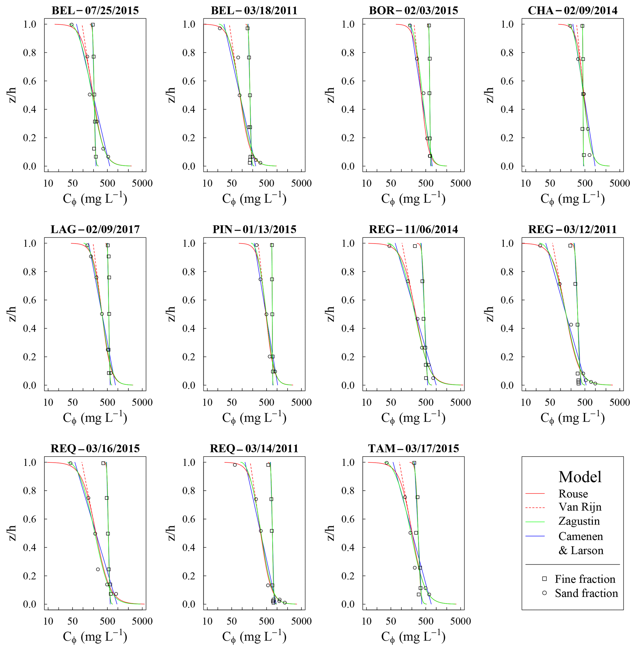
Figure 6 Typical examples of measured concentration profiles C_ϕ(z∕h), fitted with the Rouse, Van Rijn, Zagustin, and Camenen and Larson models.

The use of the Camenen and Larson model to calculate the mean concentration 〈C_ϕ〉 seems to be a reasonable approximation. Indeed, for the range of nominal Rouse numbers considered here (P_ϕ<0.6), the bottom concentration gradient has little influence on 〈C_ϕ〉 because the velocity decreases rapidly with depth in this region of the flow. Moreover, the top-layer concentrations are too low to weight significantly on 〈C_ϕ〉.

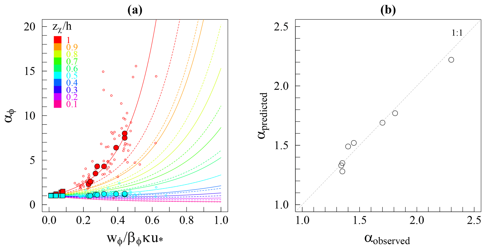
Figure 7 (a) Predicted and observed ${\mathit{\alpha }}^{{\mathit{\varphi }}_i}$ ratios as a function of the Rouse number. Filled circles and squares are the mean α_ϕ values observed per site for the sand and fine mass fractions, respectively. Unfilled circles denote observed α_s values. The red to pink rainbow set of solid lines correspond to the general model prediction (Eq. 17), and each represents 10 % of the water height. Dashed lines are for the simplified model (Eq. 18). (b) Predicted vs. observed mean α ratios per site (i.e., total concentration).

The comparison between the predicted and observed mean α_ϕ values per site and size group (Fig. 7a) allows for the validation of the general model proposed in this work (Eq. 17). To show the model's ability to predict how α_ϕ changes with flow conditions at one specific site, this model was also compared with all of the α_ϕ values observed at the water surface and at mid-depth (Fig. 7a). The observations follow the model trend well, despite the high scatter of the α_s(h,P_s) values, which is caused by the low diffusivity and concentration in coarse material near the water surface and by the uncertainty of the exact z position of the samples. At mid-depth, the α_s(0.5h,P_s) values have lower scatter.

Nevertheless, the α_s sensitivity to the Rouse number remains moderate for most of the hydraulic conditions encountered, except for the extremely low flow rates, i.e., when P_s>0.5. The α_f sensitivity to changes in flow conditions is very small. Then, considering the small contribution of the low waters to the sediment budget and the small Rouse number variations for the nominal hydraulic conditions at a specific site (Table 2), the use of the mean α_ϕ coefficients per site seems to be reasonable for assessing reliable sediment budgets. Regarding the simplified model (Eq. 18), a reasonable approximation is expected to be found in the central region of the flow, but the values gradually depart from the observations near the water surface and the riverbed.

Finally, the mean ratios α(h) per site were computed (Eq. 15) using the predicted mean α_f(h,P_f) and α_s(h,P_s) (Eq. 17) and the mean mass fractions X_f and X_s measured at the water surface (Table 2). The observed vs. predicted α ratios are in excellent agreement (r²=0.97) (Fig. 7b) and validate the prediction ability of the model when the Rouse numbers are accurately known.

4 Discussion on the model applicability

The equations proposed in this work (Eqs. 17, 18) for modeling the ratios α_ϕ(z_χ,P_ϕ) become very sensitive when both the index sample is taken near the river surface (z_χ≈h) and the Rouse number is rather large (P_ϕ>0.4) (Fig. 7a). This is a first limitation for the model applicability, if a monitoring of the index concentration at a deeper level on the water column is not technically feasible. In addition, for rivers with Rouse numbers greater than 0.6 (i.e., when the suspension does not occur in the entire water column because the particle are too coarse, in comparison to the strength of the flow, to be uplifted at the water surface), the weight of the velocity distribution in the model can no longer be neglected as it was in this work (see the assumption, Sect. 2.3.1). Furthermore, the higher the Rouse number, the more difficult the concentration measurement is to perform. Then, the accuracy of the model also depends on the concentration measurement procedure chosen and related uncertainties. These uncertainties depend on the point-sampling integration-time which must be long enough to be representative (Gitto et al., 2017), on the volume of water collected and on the sampling position(s) defined in the cross section.

Therefore, estimating P_ϕ with a low uncertainty is a key issue to predict accurate α_ϕratios during sediment concentration monitoring. This estimation can be achieved (1) via the estimation of the hydraulic parameter u_∗, w_ϕ and β_ϕ, or (2) empirically using detailed point concentration measurements. Then, if the Rouse number variability is significant during the hydrological cycle, the empirical relationship between u_∗ or h and the P_ϕ fitted on measured concentration profiles may be calibrated.

4.1 Estimation of the diffusivity ratio β_ϕ

For many decades, studies based on flume experiments or measurements in natural rivers have shown that β_ϕ usually departs from the unity. The sediment diffusivity increases (β_ϕ>1) with bedforms or movable bed configurations (Graf and Cellino, 2002; Gualtieri et al., 2017); specifically, the boundary layer thickness tends to be thin just before the bedforms crest, and then it peels off at the leeward side (Engelund and Hansen, 1967; Bartholdy et al., 2010). This trend implies there are anisotropic macroturbulent structures, with eddies that convect large amounts of sediments to the upper layers and settle further after eddy dissipation. Thus, bedforms locally modify the ratio between the laminar and turbulent stresses, inducing different lifting profile shapes in the inner region (e.g., Kazemi et al., 2017) and causing the mixing length theory to fail in the overlap region. Centrifugal forces driven by turbulent motion and applied on the grains could also enhance the particle exchange rate between eddies (Van Rijn, 1984). Conversely, the suspension is dampened (β_ϕ<1) when the large suspended particles do not fully respond to all velocity fluctuations, such as passive scalars.

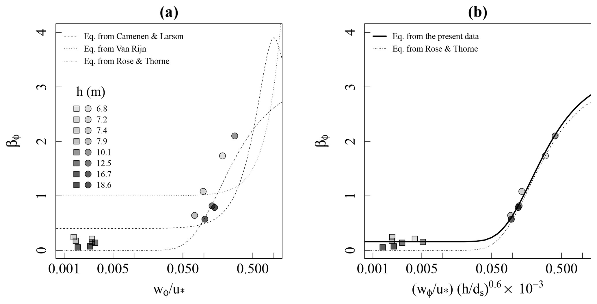
Figure 8 (a) Ratio of sediment to eddy diffusivity β_ϕ as a function of the ratio $w_{\mathit{\varphi }}/u_{\ast }$, with points shaded according to the water level h. (b) Idem, after correction of the ratio $(w_{\mathit{\varphi }}/u_{\ast })$. Circles and squares are the mean values of β_s and β_f calculated per site, respectively.

Van Rijn (1984), Rose and Thorne (2001) and Camenen and Larson (2008) attempted to model β_ϕ as a function of the ratio $w_{\mathit{\varphi }}/u_{\ast }$ for sand and silt particles. However, the measured β_ϕ encompasses poorly understood physicochemical processes as well as uncertainties and bias of the w_ϕ and u_∗ estimations, which might partly explain the shifts along the $w_{\mathit{\varphi }}/u_{\ast }$axis between the three abovementioned laws and the β_ϕ inferred in this study from measured profiles of concentration, particle diameter and velocity (Fig. 8a).

With regard to w_ϕ, a major difficulty comes from the need to divide the PSD into various size groups and to summarize each subdistribution with a single characteristic diameter (e.g., mode, median, mean), and different values of w_ϕ(d_ϕ) are calculated according to the choices made.The aggregation process is a supplementary complicating factor (Bouchez et al., 2011) but is probably not the main issue in these white rivers with little organic matter (Moquet et al., 2011; Martinez et al., 2015). Indeed, the results of Bouchez et al. (2011) are probably biased because the authors used a single diameter to summarize the entire PSD, which is highly sensitive to the flow conditions. However, this bias would not concern the sand group because the shear modulus experienced in large Amazonian rivers would prevent the formation of large aggregates. The choice of a settling law (e.g., Stokes; Zanke, 1977; Cheng, 1997; Soulsby, 1997; Ahrens, 2000; Jiménez and Madsen, 2003; Camenen, 2007) may also induce bias on w_ϕ. In these laws, the sediment density is a key parameter that is often neglected, as natural rivers comprise a diversity of minerals with contrasting density ranges.

Conversely, the shear velocity estimation also suffers from uncertainties in terms of the velocity measurements and biases that are induced by the method used (Sime et al., 2007). For instance, the departures from logarithmic velocity profiles increase with the distance to the bed (e.g., Guo et Julien, 2008) in sediment-laden flows (e.g., Castro-Orgaz et al., 2012), which could be relevant to deep Amazonian rivers. Indeed, the mixing length expansion could reach a maximum before the water surface, as the energetic eddy size cannot expand ad infinitum far from the flow zone under the influence of bed roughness because of the increasing entropy. The log-law assumptions (i.e., constant shear velocity throughout the water column and mixing length approximation) would no longer be valid, and the velocity profiles would follow a defect law in the outer region. This raises the need to find a suitable model for the velocity distribution in large rivers, leading to an unbiased estimate of the shear velocity.

Thus, it is not surprising to find discrepancies between the empirical laws and the observations based on the experimental conditions. Here, the Rose and Thorne (2001) empirical law is the closest to the observed β_ϕ (Fig. 8a), with departures that seem to be a function of the water level. We assume that a global correction of the different bias on the $w_{\mathit{\varphi }}/u_{\ast }$ term would depend on the flow depth as well as on the skin roughness, which partly influences the formation and expansion of the turbulence structures and thus influences the velocity distribution (Gaudio et al., 2010). Here, d_s is considered instead of the skin roughness height, as few riverbed PSDs are available and because it is a key parameter for the settling law. Thus, the following modification of the Rose and Thorne (2001) law is proposed:

$$\begin{array}{}\text{(19)}& {\mathit{\beta }}_{\mathit{\varphi }}=\mathrm{3.1}\exp \left[-\mathrm{0.19}\times {\mathrm{10}}^{-\mathrm{3}}{\displaystyle \frac{u_{\ast }}{w_{\mathit{\varphi }}}}{\left({\displaystyle \frac{h}{d_{\mathrm{s}}}}\right)}^{\mathrm{0.6}}\right]+\mathrm{0.16},\end{array}$$

where the coefficient 3.1 comes from the Rose and Thorne (2001) law. Other numerical values in Eq. (19) were fitted to obtain the best agreement with the β_ϕ inferred from the measured concentration profiles (Table 2). In a similar way to Camenen and Larson (2008), a minimum β_ϕ-value was found for very small values of $w_{\mathit{\varphi }}/u_{\ast }$. This nondimensional law, which extends below the range of $w_{\mathit{\varphi }}/u_{\ast }$ usually considered in previous studies, allows for an enhanced prediction of β_ϕ(±0.03) (Fig. 8b).

Furthermore, the dataset did not show any relationship between concentration and the diffusivity ratio β_ϕ (not shown here). The uncertainties in the dataset collected under field conditions do not allow for the further investigation of the influence of second-order factors on the diffusivity ratio, such as the particle characteristics (shape, grain size, density, and so on), the aggregation phenomenon or the level of stratification of the flow (e.g., Van Rijn, 1984; Graf and Cellino, 2002; Pal and Ghoshal, 2016; Gualtieri et al., 2017).

Figure 9 Fitted Rouse numbers against (a) predicted P_s (the gray square in the bottom-left represents the range of variation of P_f), (b) shear velocities and (c) water levels.

Applying Eq. (19) to predict the mean β_ϕ values per site, the predicted and fitted P_ϕ are in good agreement (Fig. 9a), with little scatter when considering the uncertainties in the measured concentrations and therefore on the fitted P_ϕ. This result shows that the shear velocity mainly controls the Rouse number variability at a given site (Fig. 9b). Therefore, the variations in particle size are a second-order factor. The shear velocity is itself driven by the high amplitude of the water depth in Amazonian rivers (Fig. 9c), and it has hysteresis effects at the gauging stations located in the floodplain, which are attributed to the backwater slope variability in these subcritical flood wave contexts (Trigg et al., 2009). Hence, the accurate monitoring of the water level and knowledge of the river surface slope, even if limited or biased, would allow for an acceptable prediction of the Rouse numbers, which could be used to establish a single β_ϕ value per site.

4.2 Predicting d_s from the riverbed PSD

For fine particles, d_f can be accurately measured in the water column because the fine particles are well mixed in the flow.

Regarding the sand particles, such measurements induce uncertainties due to the particle fluctuations in the current and because the eddy structure development in the bottom layers of the flow swiftly causes strong grain size sorting (Fig. 4). The suspended sediment particles are thus considerably smaller than the bed load or riverbed particles (Van Rijn, 1984).

The diameter of the suspended sand can be assessed by taking a representative percentile of the riverbed PSD (e.g., Rose and Thorne, 2001). Alternatively, an empirical expression that considers the flow conditions was proposed by Van Rijn (1984).

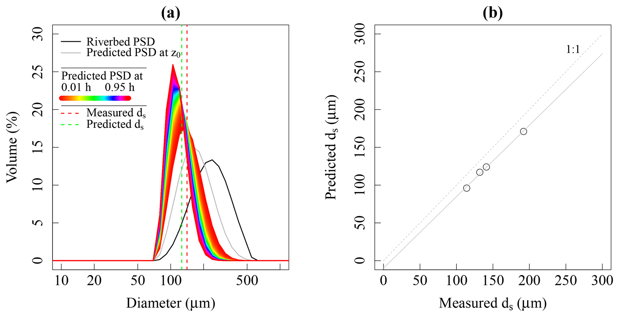
Figure 10 (a) Prediction of the mean diameter d_s at the TAM gauging station for $u_{\ast }=\mathrm{0.12}$ m s⁻¹ (mean flow conditions). (b) Predicted vs. measured d_s at BEL, REQ, REG and TAM. The dashed line denotes the first bisector, and the solid line represents the best fit.

Here, the Camenen and Larson (2005) formulae for the estimation of the reference concentration C_ϕ(z₀) was applied in a multiclass way to the riverbed PSD, and it was assumed that the size fractions did not influence each other and there was a uniform sediment density for all grain sizes (2.65 g cm⁻³). In this formulation, C_ϕ(z₀) is a function of the dimensionless grain size d_∗, the local Shields parameter θ_ϕ and of the critical Shields parameter θ_cr for the inception of transport (Camenen et al., 2014):

$$\begin{array}{}\text{(20)}& C_{\mathit{\varphi }}\left(z_{\mathrm{0}}\right)={\displaystyle \frac{\mathrm{0.0015}{\mathit{\theta }}_{\mathit{\varphi }}}{\exp \left(\mathrm{0.2}{d}_{\ast }+\mathrm{4.5}\frac{{\mathit{\theta }}_{\mathrm{cr}}}{{\mathit{\theta }}_{\mathit{\varphi }}}\right)}}.\end{array}$$

This first PSD predicted at the transition level z₀ is further diffused vertically with the Zagustin model (Eq. 19), considering the Soulsby (1997) settling law in the P_ϕ calculations (Fig. 10a). The model underestimates the measured d_s by approximately 10 % (Fig. 10b). This slight discrepancy might be explained by stochastic and ephemeral inputs of coarse bed material in the water column, which are not addressed by the suspension theory.

4.3 Sensitivity analysis and recommendations for optimized sampling procedures

The approximation error ΔP_ϕ can be evaluated at ±0.03 (from Eq. 19, Fig. 9 or Table 2) and propagated to the corresponding ${\mathit{\alpha }}_{\mathit{\varphi }}(z_{\mathit{\chi }},P_{\mathit{\varphi }}\pm \mathrm{\Delta }{P}_{\mathit{\varphi }})$ (Fig. 11a). The error on z_χ is not considered here but would increase the α_ϕ sensitivity in the zones with a high concentration gradient. Overall, the relative error on α_ϕ remains moderate for all of the flow conditions experienced by the rivers studied here (i.e., below ±10 % in the central zone of the flow and below ±20 % at the water surface), except near the riverbed (Fig. 11a). Nevertheless, for operational applications, this result must be weighted by the relative error profile of the measured index concentrations ΔC_ϕ(z_χ)∕C_ϕ(z_χ).

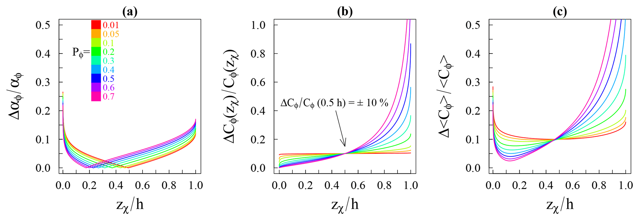
Figure 11 (a) Relative error of the predicted α_ϕ according to the relative height z_χ∕h of the index sampling, for various Rouse numbers P_ϕ. (b) Relative error of the concentration sampled, inferred from the Zagustin model and assuming $\frac{\mathrm{\Delta }{C}_{\mathit{\varphi }}}{C_{\mathit{\varphi }}}(z_{\mathit{\chi }}=\mathrm{05}h)=\pm \mathrm{10}$ %. (c) Relative error on 〈C_ϕ〉 as a function of z_χ∕h.

By substituting C_ϕ(z_χ) with the Zagustin model (Eq. 9) and assuming $\mathrm{\Delta }{C}_{\mathit{\varphi }}\left(\mathrm{0.5}h\right)/C_{\mathit{\varphi }}\left(\mathrm{0.5}h\right)=\pm \mathrm{10}$ %, it is possible to model this profile of concentration uncertainty (Fig. 11b) and to derive the relative uncertainty of 〈C_ϕ〉 according to the sampling height under various flow conditions (Fig. 11c). Here, the considered uncertainty is a simple function of the concentration. However, coarse particles are more sensitive to current fluctuations than are fine sediments. Thus, the sand concentration uncertainty is underestimated, at least in the region of the flow under bed influence $\sim \left[z_{\mathrm{0}},\mathrm{0.2}h\right]$, where stochastic uplifts of bed sediments impose high variability on the concentration. Furthermore, the sampling frequency as well as the number of index samples taken and their positions are important parameters to consider. The section geometry, the velocity distribution and the transversal movable bed velocity pattern are important guidelines in the selection of a sampling position(s). The integration of the lateral variability of the concentration is not discussed here. Nevertheless, when considering these assumptions, optimized sampling heights may be defined as follows:

• For fine sediments (P_f<0.1), the most accurate 〈C_f〉 is obtained when sampling the water column at approximately 0.5h. The sampling can also be achieved at the water surface with a good estimation of 〈C_f〉 (±15 %).

• For the sand fraction at the piedmont stations (P_s<0.3), sampling in the [0.2h,0.8h] region is recommended to keep the errors of 〈C_s〉 below ±20 %. Sampling at the water surface is still possible, but there will be uncertainties between ±20 % and 40 % for 〈C_s〉.

• For enhanced monitoring of the sand concentration at the lowland stations (P_s>0.3), the [0.2h,0.8h] zone is preferred over the water surface, where the α_ϕ prediction would require very accurate estimations of P_s and C_s(h).

The proposed α_ϕ models (Eqs. 17, 18) allow for a routine protocol with sampling in the central zone of the flow to be achieved: the α_ϕ can be predicted at each sampling time-step, when the section geometry is known and when the flow is sufficiently stable to estimate z_χ∕h. For instance, a single fixed sampling depth could be used. Alternatively, the Rouse number can be estimated at each sampling time-step from Eq. (7) by sampling two heights $z_{{\mathit{\chi }}_{\mathrm{1}}}$ and $z_{{\mathit{\chi }}_{\mathrm{2}}}$ of the water column at each measurement time-step:

$$\begin{array}{}\text{(21)}& P_{\mathit{\varphi }}={\displaystyle \frac{\ln \left(\frac{C_{\mathit{\varphi }}\left(z_{{\mathit{\chi }}_{\mathrm{1}}}\right)}{C_{\mathit{\varphi }}\left(z_{{\mathit{\chi }}_{\mathrm{2}}}\right)}\right)}{\ln \left(\frac{z_{{\mathit{\chi }}_{\mathrm{2}}}}{z_{{\mathit{\chi }}_{\mathrm{1}}}}\frac{\left(h-z_{{\mathit{\chi }}_{\mathrm{1}}}\right)}{\left(h-z_{{\mathit{\chi }}_{\mathrm{2}}}\right)}\right)}}.\end{array}$$

For instance, the concentration at $z_{{\mathit{\chi }}_{\mathrm{1}}}=\mathrm{0.7}h$ and at $z_{{\mathit{\chi }}_{\mathrm{2}}}=\mathrm{0.3}h$ results in $P_{\mathit{\varphi }}=\mathrm{0.59}\ln \left(C_{\mathit{\varphi }}\left(\mathrm{0.3}h\right)/C_{\mathit{\varphi }}\left(\mathrm{0.7}h\right)\right)$.

When considering nominal flow conditions (P_ϕ<0.6), the sampling height above the riverbed $h/e\approx \mathrm{0.37}h$ (e being the Euler number) appears to be pertinent for simplified operations, as the ratios of ${\mathit{\alpha }}_{\mathit{\varphi }}(h/e,P_{\mathit{\varphi }})$ remain interestingly close to unity (±10 %) (Fig. 7a). Thus, $\left\{{\mathit{\beta }}_{\mathrm{f}},{\mathit{\beta }}_{\mathrm{s}}\right\}\approx \left\{\mathrm{0.16},\mathrm{1}\right\}$ could be simply assumed without inducing large errors in the ${\mathit{\alpha }}_{\mathit{\varphi }}(h/e,P_{\mathit{\varphi }})$ estimations. The particles are usually present in a significant amount, and the turbulent mixing is intense (Eq. 6), while the concentration gradients are moderate, which also causes for more uncertainty regarding z_χ. Interestingly, when considering the depth-averaged velocity $\langle u\rangle \approx u(h/e)$ for velocity profiles that are logarithmic in nature, the sediment discharge on a vertical q_sϕ (g s⁻¹ m⁻²) may be expressed as follows:

$$\begin{array}{}\text{(22)}& q_{\mathrm{s}\mathit{\varphi }}={\mathit{\alpha }}_{\mathit{\varphi }}\times C_{\mathit{\varphi }}\left({\displaystyle \frac{h}{e}}\right)\times u\left({\displaystyle \frac{h}{e}}\right)\cong C_{\mathit{\varphi }}\left({\displaystyle \frac{h}{e}}\right)\times \langle u\rangle \pm \mathrm{10}\mathit{\%}.\end{array}$$

Finally, if sampling in the central zone of the flow is not technically feasible during concentration monitoring, the mean concentration of fine particles may be estimated with surface index sampling or remote sensing (Martinez et al., 2015; Pinet et al., 2017). Then, the sand concentration could be assessed with a sediment transport model that is suitable for large rivers (e.g., Molinas and Wu, 2001; Camenen and Larson, 2008). To parameterize such models, improved spaceborne altimeters (e.g., the SWOT – Surface Water Ocean Topography – mission) and hydrological models are already serious alternatives to in situ discharge, water level and slope measurements (e.g., De Paiva et al., 2013; Paris et al., 2016).

5 Conclusion and perspectives

The use of measured concentration profiles with physically based models describing the suspension of grains in turbulent flow has shown the possibility to derive a simple model for the prediction of α_ϕ, i.e., for a given particle size group ϕ. Proper modeling of the PSD using two hydraulically consistent size groups (i.e., fine particles and sand) is first required to obtain a characteristic diameter that is mostly constant for each size group during the hydrological cycle.

The Zagustin profile, with finite values at the water surface, demonstrated the best suitability in relation to the observed data. Nevertheless, the Camenen and Larson model was in good agreement with the observations in the central zone of the flow and was a reasonable approximation of the depth-averaged concentration.

The Rouse number is the main parameter for α_ϕ modeling. Variations in P_ϕ during the hydrological cycle may be monitored from a few point concentration measurements or through the calibration of a relation between the u_∗ or h and the measured P_ϕ. Alternatively, a function of $w_{\mathit{\varphi }}/u_{\ast }$ and h∕d_s was proposed to compute β_ϕ and predict P_ϕ±0.03.

The sensitivity of the α_ϕ model decreases from the boundaries to a zone between [0.2h,0.5h] which is based on the flow conditions. At the water surface, the model becomes inaccurate when P_s>0.3, i.e., for flow conditions corresponding to sand suspension in the lowland. In such a context, sampling in the central zone of the flow is preferable for sand concentration monitoring. A pertinent sampling height for optimized concentration monitoring appears to be z_χ=0.37h.

This insight into the hydraulic theory leads to enhanced sediment monitoring practices, with a more accurate estimate of the sediment load, especially in regions with limited data availability, such as the Amazon Basin. Indeed, the proposed model is a tool that can be used to predict the α_ϕ and α ratios and can also be used to select a proper sampling height for optimized monitoring. Extensively, the model allows for detailed uncertainty analysis on the 〈C〉 derived from an index method.

Finally, where the cross-section geometry is well known and where no in situ concentration data exist, the model could allow for an accurate estimation of the mean concentration in fine sediments 〈C_f〉, with remote-sensing monitoring of the index concentration in fine sediments on the water surface. Coupling this monitoring with a sand transport model suitable for large rivers could ensure a better understanding of the sediment dynamics in the Amazon Basin.

Appendix A

A1 List of notations

.f	Fine sediment particles group (0.45 µm $<d_{\mathrm{f}}<\mathrm{63}$ µm)
.s	Sand sediment group (ds>63 µm)
C	Time-averaged concentration (mg L−1)
d	Arithmetic mean diameter (m)
d∗	$d{\left(\frac{g\left(\frac{\mathit{\rho }}{{\mathit{\rho }}_{\mathrm{w}}}-\mathrm{1}\right)}{{\mathit{\upsilon }}^{\mathrm{2}}}\right)}^{\frac{\mathrm{1}}{\mathrm{3}}}$ is the dimensionless grain size
g	Gravitational force (m s−2)
h	Mean water depth (m)
ks	Nikuradse equivalent roughness height (m)
P	Rouse number (–)
qs	Time-averaged sediment discharge on a vertical (g s−1 m−2)
u	Time-averaged velocity (m s−1)
u∗	Shear velocity (m s−1)
w	Suspended sediment particle settling velocity (m s−1)
X	Mass fraction (–)
z	Height above the bed (m)
α	Ratio between mean concentration and index concentration (–)
β	Ratio of sediment to eddy diffusivity (–)
ε	Sediment diffusivity coefficient (m2 s−1)
εm	Momentum exchange coefficient (m2 s−1)
κ	Von Kármán constant (–)
υ	Kinematic viscosity (m2 s−1)
ρw	Water density (kg m−3)
ρ	Sediment density (kg m−3)
θ	Shield's dimensionless shear stress parameter (–)
θcr	Critical dimensionless shear stress threshold (–)
〈〉	Depth-integrated value

Main subscripts

.χ	Index height value
.0	Bottom reference height value
.r	Reference height value
.ϕ	Particle size group ϕ

A2 Soulsby (1997) settling law (terminal velocity)

$$w={\displaystyle \frac{\mathit{\nu }}{d}}\left(\sqrt{{\mathrm{10.36}}^{\mathrm{2}}+\mathrm{1.049}{d}_{\ast }^{\mathrm{3}}}-\mathrm{10.36}\right).$$

A3 Velocity laws

Inner law (“law of the wall”):

$$u\left(z\right)={\displaystyle \frac{u_{\ast }}{\mathit{\kappa }}}\ln \left({\displaystyle \frac{\mathrm{30}z}{k_{\mathrm{s}}}}\right).$$

Zagustin (1968) defect law:

$$u\left(z\right)=U_{max}-\mathrm{2}\times {\displaystyle \frac{u_{\ast }}{\mathit{\kappa }}}\mathrm{arctanh}{\left({\displaystyle \frac{h-z}{h}}\right)}^{\frac{\mathrm{3}}{\mathrm{2}}}.$$