the Creative Commons Attribution 4.0 License.
the Creative Commons Attribution 4.0 License.
 | 09 Dec 2020
Short communication: Multiscalar roughness length decomposition in fluvial systems using a transform-roughness correlation (TRC) approach
Andrea Zampiron
In natural open-channel flows over complex surfaces, a wide range of superimposed roughness elements may contribute to flow resistance. Gravel-bed rivers present a particularly interesting example of this kind of multiscalar flow resistance problem, as both individual grains and bedforms may contribute to the roughness length. In this paper, we propose a novel method of estimating the relative contribution of different physical scales of in-channel topography to the total roughness length, using a transform-roughness correlation (TRC) approach. The technique, which uses a longitudinal profile, consists of (1) a wavelet transform which decomposes the surface into roughness elements occurring at different wavelengths and (2) a “roughness correlation” that estimates the roughness length (ks) associated with each wavelength based on its geometry alone. When applied to original and published laboratory experiments with a range of channel morphologies, the roughness correlation estimates the total ks to approximately a factor of 2 of measured values but may perform poorly in very steep channels with low relative submergence. The TRC approach provides novel and detailed information regarding the interaction between surface topography and fluid dynamics that may contribute to advances in hydraulics, bedload transport, and channel morphodynamics.
- Article
(5521 KB) - Full-text XML
- BibTeX
- EndNote


Understanding flow resistance is of great interest to river research and practice. The estimation of flow resistance is important for determining flood magnitudes, predicting ecological habitat, estimating rates of sediment transport, and understanding channel morphodynamics. However, the hydraulics of gravel-bed channels, in particular, are relatively poorly understood (see Ferguson, 2007). Given that most of the foundational work in fluid dynamics, upon which conventional approaches to predicting flow resistance are based, was conducted using regular (e.g. Schlichting, 1936) or uni-scalar (e.g. Nikuradse, 1933) bed geometry, the multiscalar topographic characteristics of these rivers present a major challenge. In particular, individual grains and assemblages of grains (“forms”) on the bed surface, spanning orders of magnitude of scale, have variable contributions to the total flow resistance across different channel types. Thus, moving forward, mainstream empirical approaches to estimating flow resistance based solely on grain diameter would ideally be replaced by approaches that explicitly account for multiple spatial scales (see Adams, 2020a). Decomposing roughness lengths into different scales may contribute to an understanding of channel morphodynamics given that energy dissipation is increasingly recognized as a condition governing system behaviour (Eaton and Church, 2004; Nanson and Huang, 2018; Church, 2015). Also, the partitioning of bed stresses between grain and form scales is an important step in predicting bedload transport (Ancey, 2020).
Inspired by early work in fluid dynamics (Schlichting, 1936; Keulegan, 1938) and subsequent work in fluvial hydraulics (Einstein and Banks, 1950; Nowell and Church, 1979), some geomorphologists sought to disaggregate the roughness length into grain and form contributions by correlating bar geometry with flow resistance (Davies and Sutherland, 1980; Prestegaard, 1983). However, further work was likely hindered by limitations associated with the collection of topographic data in rivers (Furbish, 1987; Robert, 1988). Advances in remote sensing and statistics have since allowed researchers to explore detailed scaling characteristics of gravel-bed surfaces using analyses such as variograms (Robert, 1988; Clifford et al., 1992) and transforms (Nyander et al., 2003). Topographic analyses have led to multiscalar decompositions of geometric roughness in rivers, although to our knowledge, full decompositions of hydraulic roughness have not yet been presented. The latter approach has been developed for complex aeolian surfaces using transforms (Nield et al., 2013; Pelletier and Field, 2016; Field and Pelletier, 2018), which serves as a proof of concept for a multiscalar roughness length decomposition.
In a review of flow resistance in gravel-bed rivers, Adams (2020a) identified two relatively recent advancements in the fields of statistics and fluid dynamics that could contribute to a multiscalar roughness length decomposition tool. The first advancement is the wavelet transform, which is generally superior to the Fourier transform when analysing the underlying structure of complex and aperiodic signals. This is due to the use of a finite (rather than a continuous) wavelet function, which gives rise to a family of wavelets that are dilated (stretched and compressed) and translated (shifted) along the signal (Torrence and Compo, 1998). There are now various types of wavelet transforms suited to different applications, some of which have been applied in rivers (Kumar and Foufoula-Georgiou, 1997; Nyander, 2004; Keylock et al., 2014). The second advancement is the development of roughness correlations for irregular surfaces (e.g. Forooghi et al., 2017; De Marchis et al., 2020), which estimate the roughness length of a surface based purely on its geometric characteristics.
In this study, we present a novel method of estimating the relative contribution of different physical scales of river bed topography to the total roughness length based on longitudinal profiles. The general approach consists of (1) a wavelet transform in which the channel surface is decomposed into a set of more simple components each at a different wavelength and (2) a roughness correlation that estimates the roughness length associated with each wavelength, which is expressed as the equivalent sand roughness parameter ks (Nikuradse, 1933; Schlichting, 1936). By modifying the specific roughness correlation that is used, the transform-roughness correlation (TRC) approach may be applied across a wide range of channel types and hydraulic conditions. To demonstrate the TRC analysis, we apply it to a series of original laboratory experiments with high-resolution digital elevation models (DEMs), as well as some additional published data.
The transform-roughness correlation approach is a generic tool that should be adapted based on the hydraulic conditions and the purpose of its application. These considerations should span the dataset, the type of wavelet transform, and the specific roughness correlation that is selected. We first discuss these general considerations to provide important context for the TRC approach, prior to introducing the experimental data and the Forooghi et al. (2017) roughness correlation in Sect. 3.2.
First, the minimum resolution and spatial extent of the topographic dataset should be informed by the scale of the features of interest. The data should have a sufficiently high spatial resolution such that they can capture the range of in-channel features that produce drag. Also, to capture the characteristic geometry of bed features (notably, height and spacing) and estimate a reach-averaged roughness length, the spatial extent of the dataset should be at least the length of the largest features that influence the flow; for example, it should span a series of dune crests or pool–riffle pairs.
Second, given that the hydraulic roughness of in-channel features is of interest, the channel topography can be reduced to a one-dimensional profile extending along the thalweg, representative of the primary flow path. It is important to note here that this approach ignores resistance elements, such as channel planform, and three-dimensional interactions between flow and in-channel topography. If both hydraulic and topographic data are available, this assumption may be validated by comparing the roughness length estimated using the roughness correlation to a measured roughness length (see Sect. 3.1.2). If the range of interactions between the flow and the surface is of interest, multiple parallel elevation profiles could be analysed.
Third, the choice between discrete and continuous wavelet transforms (DWT and CWT) is a trade-off between the resolution of the decomposition and the physical resemblance to the original profile. Compared to the DWT, the CWT extracts more intricate structural characteristics from the signal and yields a greater number of wavelengths between which information is shared (Addison, 2018). However, the redundancy in the CWT generates a more abstract representation of the topographic variation at a given wavelength. In Fig. 1, we compare wavelengths extracted using a maximal overlap discrete wavelet transform (MODWT) and a CWT using the same elevation profile. At the wavelength corresponding to the spacing of a pool–bar–riffle sequence (λ≈2 m), the oscillations output by the MODWT are aligned with the pool–riffle undulations (i.e. the position of peaks and the general shape are similar), but the CWT oscillations do not appear to align with the original profile. Given that they do not resemble the channel surface, it may be invalid to infer hydraulic behaviour from CWT wavelengths.
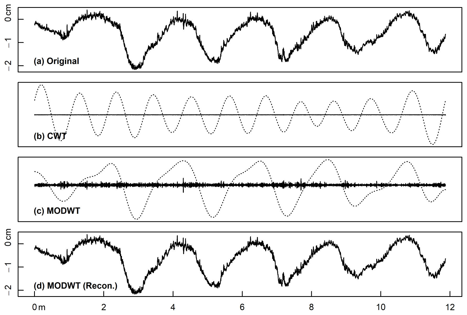
Figure 1(a) Thalweg elevation profile at end of Experiment 1a (this study) featuring a prominent pool–riffle sequence, where the x axis represents distance upstream, (b) grain (λ=4 mm) and form (λ≈2 m, dashed line) wavelengths derived from CWT, (c) the same two wavelengths derived from a MODWT, and (d) the original signal reconstructed from the MODWT by recombining wavelengths.
Fourth, the specific roughness correlation that is used should match the regime of the channel's boundary Reynolds number , where U* is shear velocity, k is a representative roughness scale, and v is kinematic viscosity. For example, given that gravel-bed rivers tend to be within the fully rough regime where (e.g. Buffington and Montgomery, 1997; Schlichting, 1979), it may only be valid to apply roughness correlations obtained for that regime specifically. Also, the flow should be turbulent, and it should be two-dimensional, which may be indicated (although not guaranteed) by flow aspect ratios (w∕h, where w is the wetted width and h is flow depth) greater than 5 (Nezu and Nakagawa, 1993).
Last, roughness correlations in fluid dynamics tend to be developed for flows sufficiently deep to have logarithmic velocity profiles, which should be considered when they are applied to flows with less developed profiles. Jimenez (2004) suggested that logarithmic layers develop where relative submergence h∕k is greater than 40, although Cameron et al. (2017) observed a logarithmic layer in rough open-channel flow at submergences as low as 1.9. During most flow conditions, it is common for gravel-bed rivers to have relative submergences of less than 10 and, in some cases, as low as 0.1 (Lee and Ferguson, 2002; Ferguson, 2007), where no logarithmic layer can develop because roughness elements are not submerged. However, if one is interested in channel-forming flows capable of reworking the bed surface (Ashworth and Ferguson, 1989; Wolman and Miller, 1960) where relative submergence may be 2 orders of magnitude higher (Limerinos, 1970; Bray, 1982), the logarithmic assumption should be satisfied for most rivers.
3.1 Stream table experiment
To demonstrate the TRC approach, we required a large set of DEMs and associated hydraulic data for validation and ideally straight channels where in-channel features represent the dominant source of drag. We conducted a set of experiments using the Adjustable-Boundary Experimental System (A-BES) at the University of British Columbia (Fig. 2). The A-BES comprises a 1.5 m wide by 12.2 m long tilting stream table and a recirculating water pump controlled by a digital flow meter. The experiments were run as generic Froude-scaled models with an initial bed slope of 2 % and a length scale ratio of 1:25, based on field measurements Fishtrap Creek in British Columbia, Canada. The bulk material ranged from 0.25 to 8 mm (Dmax), with a D50 of 1.6 mm and D84 of 3.2 mm (see MacKenzie and Eaton, 2017), and the grain size distribution (GSD) is included in Fig. 6.
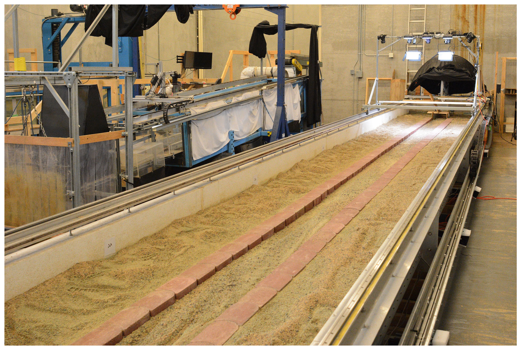
Figure 2Adjustable-Boundary Experimental System (A-BES) at the University of British Columbia, showing the camera rig and the 30 cm wide channel configuration.
3.1.1 Experimental procedure
Roughly cast interlocking concrete bricks were configured to make two straight channels of different widths: (1) a 30 cm wide configuration that represents the scaled width of the field prototype and (2) an 8 cm wide configuration which was selected based on preliminary experiments where channel width was decreased until bar formation was suppressed entirely. Thus, the two widths yield a range of bed morphologies and hydraulic conditions.
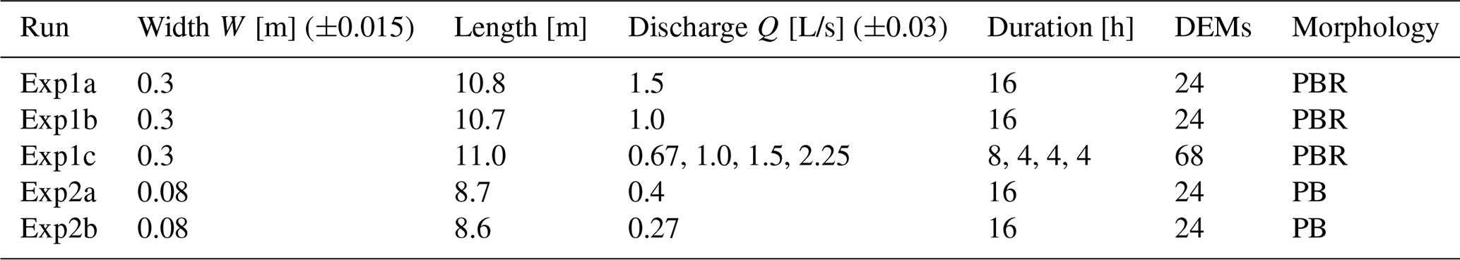
A set of experiments was carried out for each configuration (Table 1), yielding two broad types of in-channel morphology: (1) pool–bar–riffle (PBR), consisting of a gently meandering, undulating thalweg with alternate bars, and (2) plane bed (PB), with no discernible morphology beyond the grain scale. The first experiment (“a”) consisted of a formative discharge (1.5 L/s for the 30 cm channel) for a duration of 16 h, where the discharge was scaled by the width of the experimental channel W. The second experiment (“b”) consisted of a flow two-thirds of the formative discharge for 16 h. The third experiment (“c”), conducted for the 30 cm wide channel only, consisted of low flow for 8 h and then three 4 h phases with discharge increasing by a factor of 1.5 each time.
Table 1Summary of experimental conditions in the A-BES. Length refers to the median length of DEMs, which generally varies by ±0.1 m and does not include approximately 20–30 cm of bed at the upstream end. The DEM count excludes the screeded bed which has no associated hydraulic data.
Before each experiment, the bulk material was hand-mixed to minimize downstream and lateral sorting, and the channel area was screeded to the height of weirs at the upstream and downstream end. The flow was run at a low rate (at which there was little to no movement of sediment) until the bed was fully saturated and was then rapidly increased to the target flow. At the downstream end, where water free-falls over the weir, there was slight and localized lowering of the water surface due to a downdraw effect but no discernable backwater. Each period of constant discharge was divided into phases of increasing duration, between which the bed was rapidly drained (to minimize the potential for morphologic change), photographed, and re-saturated before resuming the experiment. Phases for the 16 h experiments consisted of 5, 10, 15, 30, 60, and 120 min, with four repeats of each. The 4 and 8 h periods of constant discharge followed the same sequence but did not include the longest phases. In the final 30 s of each phase, the water surface elevation was recorded at each gauge to the nearest 1 mm. Water gauges were read at an almost horizontal angle, which in conjunction with the dyed blue water, minimized systematic bias towards higher readings due to surface tension effects.
The camera rig consisted of five Canon EOS Rebel T6i DSLRs with EF-S 18–55 mm lenses, positioned at varying oblique angles in the cross-stream direction to maximize coverage of the bed, and five LED lights. Photos were taken in RAW format at 20 cm intervals, yielding a stereographic overlap of over two-thirds. Throughout the experiment, sediment collected in the trap was drained of excess water, weighed wet to the nearest 0.2 kg, placed on the conveyor belt at the upstream end, and recirculated at approximately the same rate it was output. Zero sediment was fed into the system during the first 5 min phase. For the 5 and 10 min phases, recirculation occurred at the end of the phase, and for the phases of longer duration, recirculation occurred every 15 min regardless of whether the bed was drained.
3.1.2 Data processing
Using the images, point clouds were produced using structure-from-motion photogrammetry in Agisoft Metashape Professional 1.6.2 at the highest resolution, yielding an average point spacing of around 0.25 mm. Twelve spatially referenced control points (and additional unreferenced ones) were distributed throughout the A-BES, which placed photogrammetric reconstructions within a local coordinate system and aided in the photo-alignment process. The point clouds were imported into RStudio where inverse distance weighting was used to produce DEMs at 1 mm horizontal resolution. Despite the use of control points, the DEMs contained a slight arch effect whereby the middle of the model was bowed upwards. This effect was first quantified by applying a quadratic function along the length of the bricks, which represent an approximately linear reference elevation (brick elevations vary by ±4 mm). The arch was then removed by determining correction values along the length of the DEM using the residuals, which were then applied across the width of the model.
At two points in time across the experiments, Exp1a T60.1 (5 h 0 min) and Exp1c Phase 2 T30.3 (3 h 30 min), due to errors during photo collection or the photogrammetry processing, the DEMs were slightly shorter at the upstream end (9.4 and 7.9 m in length, respectively). These DEMs were still sufficiently long to include most of the bed topography and stream gauges and have been included in the following analysis.
We estimated the position of the channel thalweg in the 30 cm experiments by manually locating pool centroids and using Gaussian kernel regression to smooth the vertices between the centroids. An example of the estimated thalweg location is shown in Fig. 3. Given the absence of bars, the thalweg elevation profile of the 8 cm experiments was assumed to be the channel centreline.
By determining the position of stream gauges within the DEM, 10 wetted cross sections were reconstructed using the water surface elevation data (assuming a relatively horizontal water surface elevation), which were then used to estimate reach-averaged hydraulics. Mean hydraulic depth was calculated as , where A is cross-sectional area and w is the wetted width. Velocity was estimated using the continuity equation . Shear velocity is , where g is gravity and S is mean bed slope, and Froude number . Based on the measurement precision of stream gauge readings, errors of 6 %–11 % could be expected for mean hydraulic depths (relative errors are variable due to different depths), with a median of ±7.6 %. Accounting for the propagation of error from discharge and gauge readings, we estimate that the ratio has a median error of ±11.5 %, with a maximum of ±15 % for the shallowest depths. A summary of reach-averaged hydraulic data is presented in Table 2.
To obtain an estimate of ks using the hydraulic data (), we used a Colebrook–White type formula defined as
where K1=2.03, K2=11.09, and K3=3.41 as determined by Keulegan (1938) and Re is the Reynolds number. We neglect the second term within the logarithm as it represents the contribution of viscous forces to friction, which is likely small for hydrodynamically rough conditions. The Darcy–Weisbach friction factor f is defined as
Table 2Summary of A-BES experimental data collected during the final portion of each experimental phase. Values represent the mean of the last five measurements. The reported σz values were calculated following the detrending process detailed in Sect. 3.2, and Re* was calculated with k=D84. The roughness length is defined in Sect. 3.2. Units: W [m], Q [L/s], h [m], U [m/s], U* [m/s], σz [m], [m].
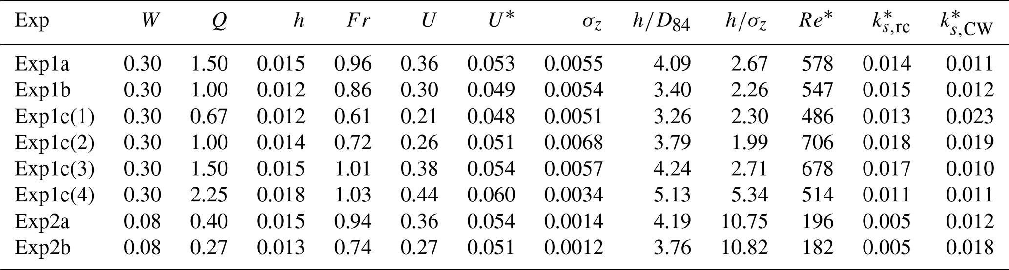
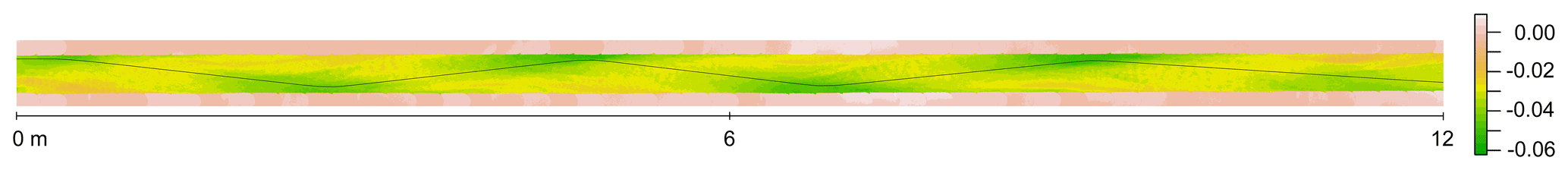
Figure 3DEM of the pool–bar–riffle channel morphology at the end of Experiment 1a, with estimated position of the thalweg. Zero represents the downstream extent of the model.
3.1.3 Additional experiments
In addition to the experiments conducted for this study, we obtained topographic and hydraulic data for 86 step–pool experiments published by Hohermuth and Weitbrecht (2018). The experiments were conducted in a 1:20 Froude-scaled model of a mountain stream, utilizing a range of bed slopes (8 %–11 %), channel widths (0.15–0.35 m), and unit discharges (0.019–0.167 m2/s). Four different grain size distributions were used, where D50 varied from 2.1–7.0 mm, and D90 remained around 58 mm. For a given experiment, a range of potentially usable elevation profiles were identified based on criteria for erroneous values; then the profile closest to the channel centreline was selected. Of the 86 experiments conducted, 83 experiments are used in this study. Thus, there is a total of 247 DEMs with associated hydraulic data when combined with the A-BES experiments.
3.2 The transform-roughness correlation approach
Here we specifically tailor the TRC approach to the geometric and hydraulic characteristics of gravel-bed channels. First, a MODWT was applied to the thalweg elevation profiles of each DEM, yielding a set of simplified profiles representing topographic variation occurring at different wavelengths. Second, we selected a roughness correlation developed by Forooghi et al. (2017) that predicts ks from surface geometry in the fully rough regime, which was applied to each wavelength. The relation was developed by conducting 38 direct numerical simulations in closed channels with an array of systematically varied roughness geometries, both regular and irregular. By correlating surface and flow properties, Forooghi et al. (2017) proposed the following empirical relation:
where kref=4.4σz and Sk is the skewness of the probability distribution of elevations. The functions F(Sk,Δ), F(Sk), and F(ES) are defined, respectively, as
and
where Δ is a measure of variability in the elevation of the peaks of roughness elements (height range divided by the mean; Δ=0 if peak heights are identical), Δ0=0.35 (not related to the critical ES value introduced below), and . The parameter ES is the effective slope, given by
where z(x) is the height array, x is the streamwise direction, and L is the surface length in x. Effective slope may be interpreted as the mean gradient of the local roughness elements (Napoli et al., 2008) and therefore represents the aspect ratio of roughness elements rather than their vertical height. With other surface parameters kept equal, the roughness length is strongly dependent on ES within the range (Napoli et al., 2008; Schultz and Flack, 2009). We calculated values of Δ for each wavelength by identifying peaks of the oscillations and found that Δ>1 for almost all cases. Values of Δ could not be estimated for the longest few wavelengths as they typically contain very few (or even one) complete oscillations that could be interpreted as roughness peaks. As a result, we simply used the F(Sk) term in Eq. (4). The roughness length for each wavelength is expressed as ks,rc.
In addition to applying the roughness correlation to each wavelength, we applied it to each thalweg elevation profile to obtain an estimate of ks, expressed as . For this calculation, each profile was detrended using a quadratic function to remove any hydraulically irrelevant large-scale variation that σz may be sensitive to. Further detrending is not necessary with the wavelet transform as the overall trend is represented by a single wavelength and removed from all others. The experimental data and code that performs the MODWT and applies the roughness correlation are available online. In the following section, we present the results of the TRC approach applied to the experiments.
In this section, we first seek to validate the TRC approach, and then focus on the multiscalar roughness length decomposition of Experiment 1a, which features a well-developed pool–bar–riffle sequence under a formative discharge. First, we compare the topographically and hydraulically based estimates of ks. Second, we demonstrate the relationship between estimates of ks with and without the wavelet transform. Third, we show how the key parameters of the roughness correlation (standard deviation, effective slope, skewness) vary across each wavelength. Fourth, we estimate the relative contribution of different scales of bed topography to the total roughness length and explain how the estimated values relate to the key parameters and the characteristics of the experiments. Fifth, we compare the performance of different roughness lengths in estimating flow resistance. Finally, we discuss the significance, limitations, and potential applications of the TRC approach.
4.1 Estimates of total ks
The relationship between the estimates of ks from the roughness correlation and the Colebrook–White equation differs between the three different channel morphologies (Fig. 4). Here, we consider to be a “measured” quantity which the roughness correlation may be tested against. The pool–bar–riffle experiments (W=0.3 m) exhibit the closest relationship between the two ks estimates, with the distribution centring along the 1:1 line (median ). The close relationship between the two independent estimates of ks supports the one-dimensional approach for these experiments as it indicates that the single elevation profile captures the roughness elements that contribute the greatest resistance to flow. Also, the results support the application of the Forooghi et al. (2017) roughness correlation to the A-BES experiments, which have more complex surface characteristics and far lower values of relative submergence compared to the numerical domain within which the correlation was developed.
The distribution of plane-bed experiments (W=0.08 m) overlaps with the 1:1 line, although there is a consistent under-prediction of ks using the roughness correlation by a factor of 2 or 3 (median ). In the case of the step–pool experiments, there is a significant under-prediction of ks by the roughness correlation of around 1 order of magnitude (median ), which may be explained with the lower relative submergence (median ).
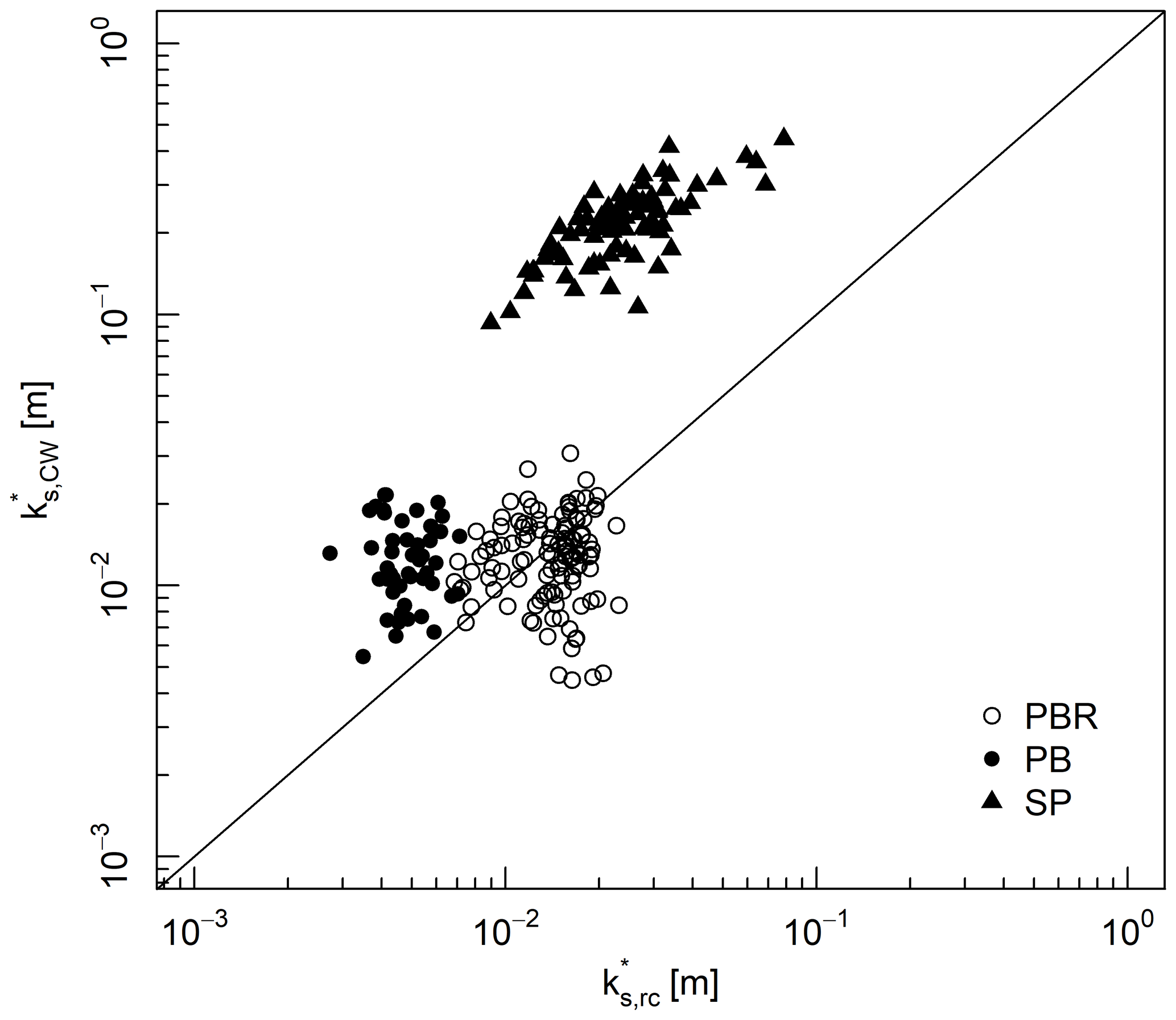
Figure 4Relationship between total ks estimated by the Forooghi et al. (2017) roughness correlation (Eq. 3) and the Colebrook–White approach (Eq. 1). Data for the A-BES experiments are grouped by channel morphology (Table 1), and the Hohermuth and Weitbrecht (2018) step–pool (SP) experiments are included.
The next stage in validating the TRC approach is comparing the values of and Σks,rc, whereby the latter is the estimate provided by applying the roughness correlation to each wavelength (giving values of ks,rc), and then taking the sum. In other words, this is comparing the values of ks estimated by the roughness correlation with and without the wavelet transform as an intermediate stage. This comparison is important for two reasons. First, the TRC approach is an extension of the linear superposition approach, which assumes that the hydraulic effect of adding up different roughness elements is approximately linear (Millar, 1999; Wilcox and Wohl, 2006; Rickenmann and Recking, 2011). In practice, superimposing roughness elements may have non-linear feedback effects (Yen, 2002; Li, 2009; Wilcox and Wohl, 2006), such that and Σks,rc may potentially not be correlated.
Second, values of and Σks,rc may differ as the process of signal decomposition and recomposition is characterized by wave interference. For example, for each thalweg elevation profile there are two estimates of amplitude: (1) the standard deviation of elevations σz and (2) Σσλ, which is the sum of σz for each wavelength. However, due to positive and negative wave interference, σz and Σσλ may significantly differ. Decomposing and recombining wavelengths alters the position and magnitude of peaks and troughs in the wavelengths and, therefore, their amplitude. Similarly, wave interference may potentially confound estimates of ks if a transform is used. For the above two reasons, it is important to demonstrate that values of and Σks,rc are correlated even if they are unlikely to have the same absolute value.
The transform and non-transform estimates of ks are positively correlated with a power-law relation (Fig. 5). It is worth noting that the two datasets are characterized by different slopes and intercepts, which may be explained with the specific characteristics of each topographic dataset (e.g. geometry, resolution) giving rise to different patterns of wave interference. However, it appears that non-linear superposition effects and wave interference do not invalidate the TRC approach for these datasets.
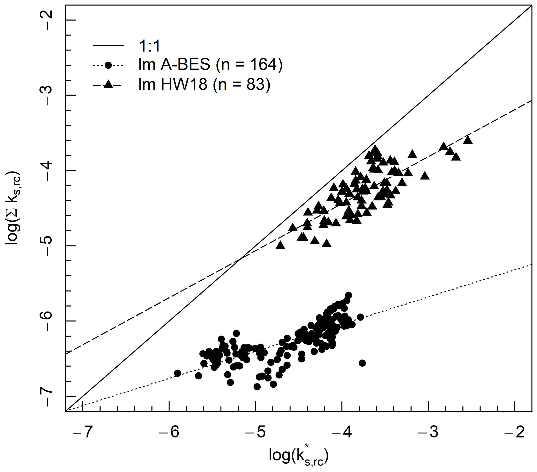
Figure 5Relationship between and Σks,rc for the A-BES and Hohermuth and Weitbrecht (2018) experiments.
4.2 Application of TRC approach
In Experiment 1a there is a general increase in the standard deviation of elevations with increasing wavelength (Fig. 6a). Over the first 10 min (i.e. the first three elevation profiles), there is an increase in σz at λ>0.5 m, with the greatest increase at λ≈2 m, but smaller wavelengths remain largely unchanged. At the smallest wavelengths, the σz tends towards zero, and there is some contribution to σz at the largest wavelengths due to the slightly concave shape of the profile, evident in Fig. 1a. Figure 6b presents the value of σz for each wavelength as a cumulative percentage. This type of graph is similar to the form size distribution (FSD) proposed by Nyander et al. (2003), which is the cumulative variance of each wavelength calculated using a 2D DWT. For comparison, we provide the bulk grain size distribution within the same space (where wavelength is grain diameter). Grain-scale wavelengths account for less than 5 % of all topographic variation, given that the arrangement of grains contribute to bed structures that usually exceed the amplitude of individual grains.
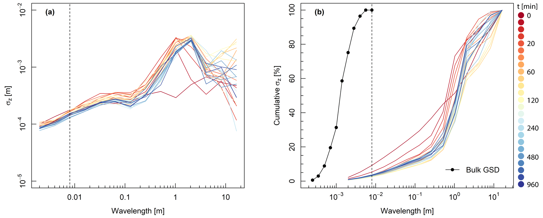
Figure 6Form size distribution during Experiment 1a, where each line represents a point in time and the initial screeded bed is included. The standard deviation of each topographic wavelength is presented as an (a) absolute and (b) cumulative percentage, for each thalweg elevation profile. The bulk grain size distribution is included, where the wavelength corresponds to grain diameter. The vertical dashed line represents the largest grain diameter in the experiment.
The effective slope is greatest at the grain-scale wavelengths () where the surface is characterized by closely bunched peaks and troughs associated with individual grains (Fig. 7a). Values of ES decrease with increasing λ, due to the presence of more gently undulating roughness elements. This is evident in the example (Fig. 1c), where the 4 mm wavelength has high ES indicated by sharp oscillations (but low σz), and the 2 m wavelength has low ES (but high σz). The main exception to the downwards trend of ES with increasing λ is the wavelength of around 2 m where there is a prominent peak in the ES distribution, associated with the development of the pool–riffle–bar sequence approximately 10 min into the experiment. Note that most of the topographic wavelengths have values of ES (and ks∕k in Eq. 3) that are smaller than the surfaces used by Forooghi et al. (2017) to develop the roughness correlation. Short wavelengths tend to be positively skewed, moderate wavelengths ( m) tend to be negatively skewed, and long wavelengths are either positively or negatively skewed (Fig. 7b). There is little change in the pattern of skewness over the course of the experiment.
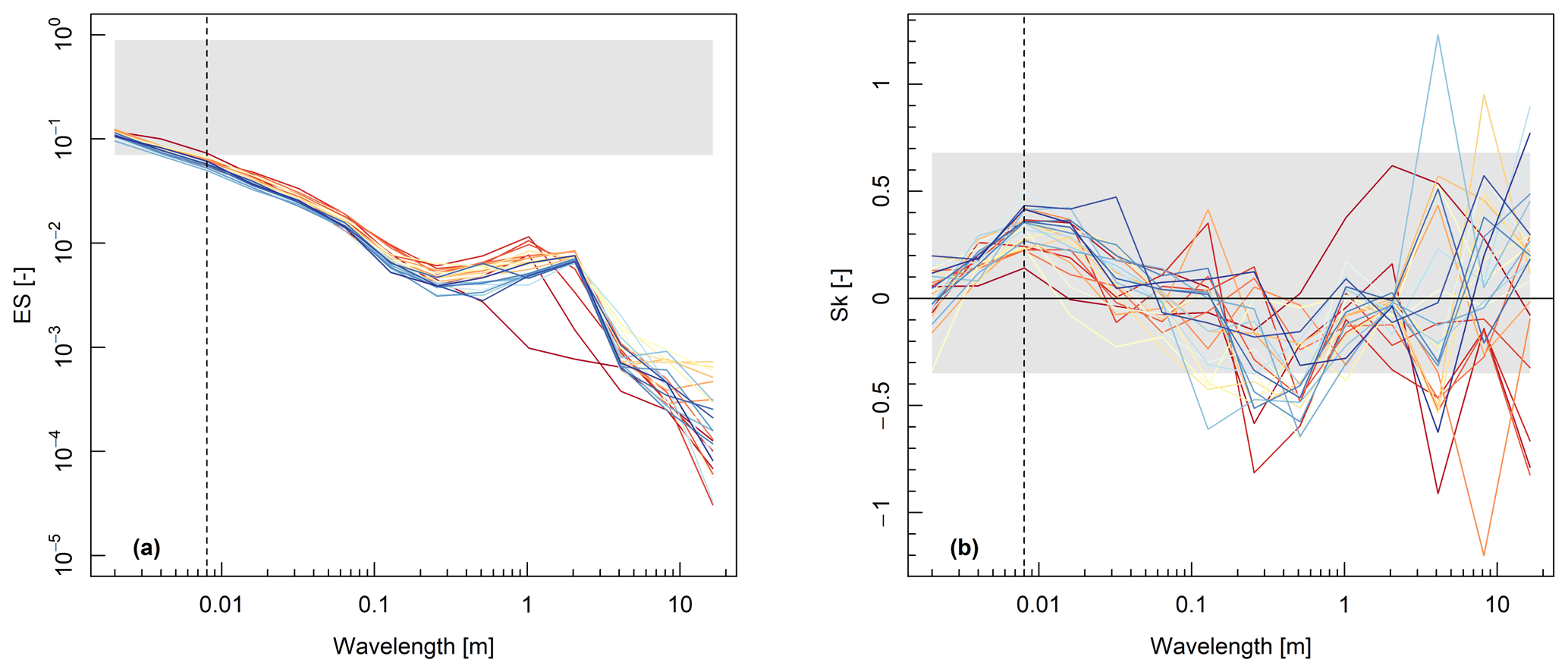
Figure 7(a) Effective slope and (b) skewness of each topographic wavelength during Experiment 1a. The shaded area represents the range of ES and Sk values of the surfaces generated by Forooghi et al. (2017). Refer to Fig. 6 for legend.
The distribution of ks,rc values predicted for each wavelength using Eq. (3) is presented in Fig. 8a. Following the format of “grain size distribution” and “form size distribution”, we term this style of plot the “drag size distribution” (DSD). There is a major peak in the DSD at λ≈2 m (the spacing of pools, bars, and riffles) and a minor peak at the scale of λ≈0.008 m (around the size of the largest grains). At small wavelengths, and large wavelengths especially, estimated ks tends downwards. Figure 8b presents the DSD as a cumulative percentage, which shows that the ks associated with the grain scale is estimated to account for approximately 30 % of the total ks. This proportion of grain and form drag is similar to estimates in gravel-bed rivers with similar morphologies (Hey, 1988; Parker and Peterson, 1980; Prestegaard, 1983), which further indicates that the TRC approach provides a physically realistic decomposition of the roughness length.
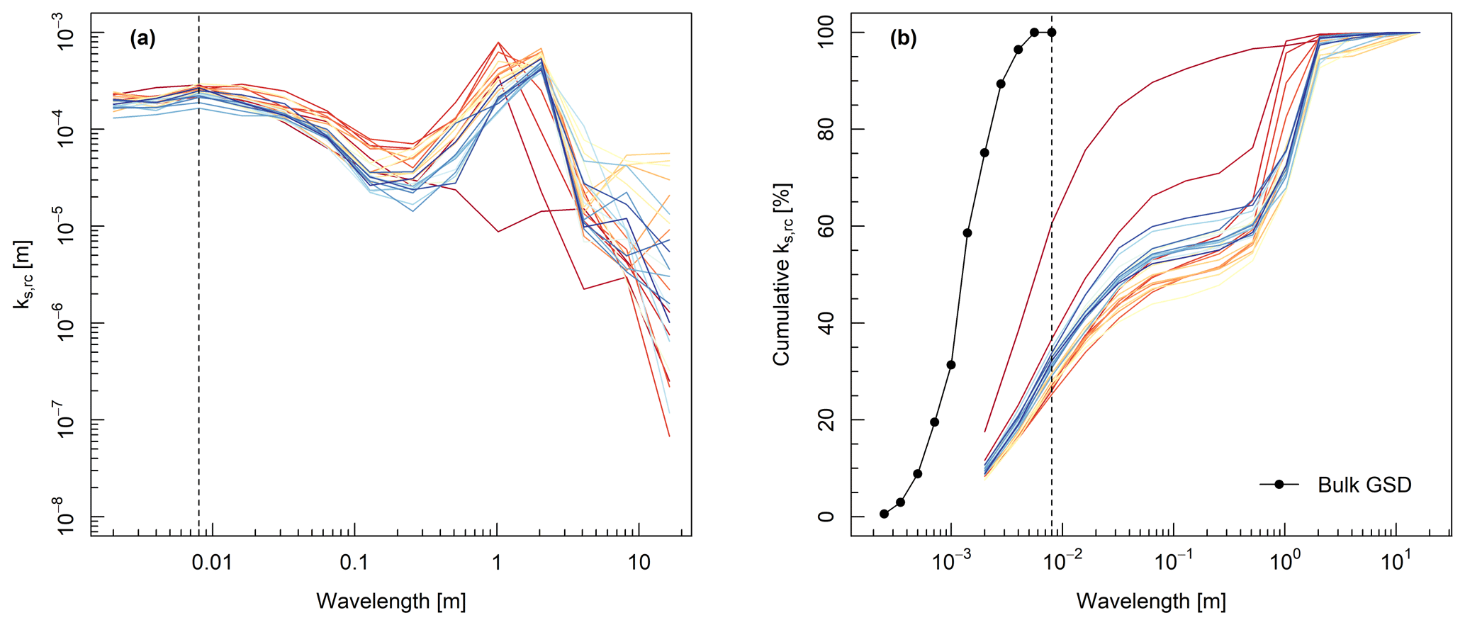
Figure 8Drag size distribution over the course of Experiment 1a. The estimated roughness length of each topographic wavelength presented as an (a) absolute and (b) cumulative percentage. Refer to Fig. 6 for legend.
In Fig. 9 we compare the performance of geometric (D84, σz) and hydraulic (, ) estimates of roughness length in estimating flow resistance, using the Ferguson (2007) variable-power equation (VPE, Appendix A). We provide two fitted relations for the VPE that provide baselines for comparison: (1) coefficients determined by a systematic review of σz as a roughness measure (Chen et al., 2020) and (2) values which are back-calculated from the hydraulic measurements. Given that these two relations represent geometric and hydraulic approaches to estimating roughness, they describe significantly different relationships between the friction factor and relative submergence.
There is a weak relationship between f and h∕k if k is estimated by the bulk D84 values (as an approximation of the surface GSD). Using σz as an estimate of k, the step–pool experiments align with the VPE relation provided by Chen et al. (2020), but σz overestimates k in the A-BES experiments. Using estimates of ks from the roughness correlation, the values of relative submergence for the A-BES experiments are consistent with the Colebrook–White relation, but there is an under-prediction of ks in the step–pool experiments. These results suggest that estimates of ks from roughness correlations may provide better estimates of flow resistance in some conditions. The results also affirm that roughness metrics derived from surface topography are superior to ones derived from the grain size distribution.
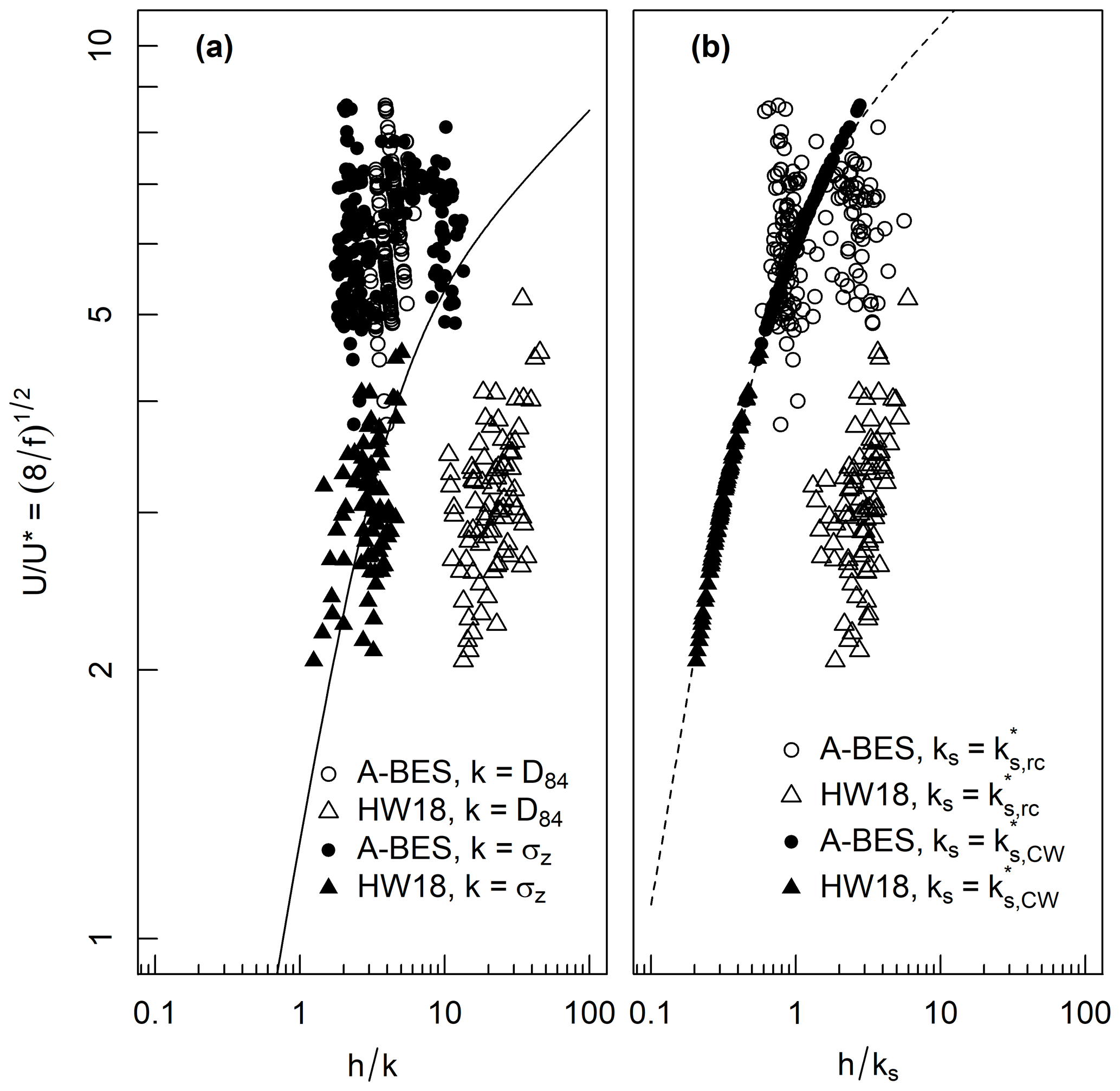
Figure 9Plot of against relative submergence for A-BES and Hohermuth and Weitbrecht (2018) data, using four different roughness lengths (D84, σz, , ). The solid line is the Ferguson (2007) VPE using coefficients a1=3.94 and a2=1.36 determined by a systematic review of σz as a roughness measure (Chen et al., 2020). The dashed line is the VPE fitted to the data, yielding coefficients of a1=7.22 and a2=11.19.
Recently proposed roughness correlations in fluid dynamics (e.g. Forooghi et al., 2017; De Marchis et al., 2020) incorporate information regarding both the height of the roughness elements (a vertical roughness scale, e.g. σz) and the arrangement or spacing of roughness elements (a horizontal roughness scale, e.g. ES). In isolation, either one of these roughness metrics may contribute to an incomplete – and potentially misleading – estimate of flow resistance. It is important to recognize that, depending on the surface of interest, the total roughness length is usually a compromise between vertical and horizontal roughness scales of the bed surface.
In gravel-bed rivers, which are typically ungauged, and where measurement of hydraulic variables is subject to practical limitations (Miller, 1958), flow resistance is usually estimated using only a vertical roughness scale such as grain diameter (Hey, 1979; Ferguson, 2007). However, the relationship between grain diameter and flow resistance breaks down in natural channels for two main reasons (see Adams, 2020a): (1) grain diameter does not account for larger and often more dissipative roughness elements, and (2) it does not consider the horizontal spacing of these larger roughness elements, which has a systematic effect on the flow (Morris, 1955; Leonardi et al., 2007). In recent years, the increased availability of high-resolution topographic data has led to the adoption of σz as a roughness metric in gravel-bed rivers, on the basis that it includes information regarding larger-scale bed structures (Chen et al., 2020). However, σz only improves upon the first deficiency of grain-based roughness metrics and, consequently, it has inherent limitations. The roughness correlation presented by Forooghi et al. (2017) may improve upon existing roughness metrics used in gravel-bed rivers, and it may be applied to most datasets where σz is calculated.
The TRC analysis has direct applications across geomorphology. Quantification of scale-dependent patterns of channel topography and roughness length may contribute to form- and process-based classifications of channel morphology and dynamics. There have been numerous attempts to classify channels based on in-channel features and their associated processes (e.g. Montgomery and Buffington, 1997); however, analysis of bed topography is typically qualitative. We expect that different channel types exhibit distinctive scale-based patterns of σz and ks, which would enable a quantitative and heuristic classification index.
The scale-based decomposition of ks may assist in identifying and forecasting the hydraulic influence of specific roughness elements in channels. For example, through the manipulation of spatial datasets by the addition or removal of features, the role of natural in-channel features (e.g. large wood) and engineering designs (e.g. rock chutes) could be isolated and determined for flood conditions. Also, multiscalar roughness length decomposition may contribute to an understanding of bedload transport processes, where accurate predictions rely on partitioning bed stresses between grain and form scales (Ancey, 2020).
However, in its current form, there are some conditions in which the TRC approach is limited. The discrepancy between topographic and hydraulic estimates of ks for step–pool channels highlights the potential limitations of the roughness correlation in steep gravel-bed rivers where slope and relative submergence have a greater hydraulic influence. In channels with significant planform resistance, the approach may require modification to account for the slope and curvature of the channel. In multi-thread channels, several profiles may need to be employed and the results weighted according to the size of the channel. Even under such conditions, multiscalar roughness length decomposition may still have considerable value with appropriate research questions and interpretation.
The transform-roughness correlation approach estimates the relative contribution of various scales of in-channel topography to the total roughness length. By modifying the roughness correlation to suit the hydraulic conditions, multiscalar roughness length decomposition may be achieved in virtually any type of river or numerical model and perhaps boundary layers in other environments. The only requirement is that the topographic data are of a sufficient resolution and spatial extent to capture the scales over which the roughness elements occur, and data of this quality are only becoming more available to geomorphologists. In particular, we expect that given the continual advances in methods for collecting bathymetric data in both shallow (Kasvi et al., 2019) and deep channels (Dietrich, 2017), applying the TRC approach will become increasingly practical in natural rivers.
Given that the TRC approach provides novel and detailed information regarding the interaction between surface topography and fluid dynamics, it may contribute to advances in hydraulics, channel morphodynamics, and bedload transport. Estimates of ks from roughness correlations may provide more immediate benefits by improving upon representative roughness values in estimating flow resistance. We are currently conducting experiments to further develop and apply these ideas.
Data and code are available online (https://doi.org/10.5281/zenodo.4116501, Adams, 2020b).
DLA was responsible for conceptualization, investigation, formal analysis, and writing. AZ provided expertise in open-channel flow, contributing to the interpretation and communication of the results and the proposed technique.
The authors declare that they have no conflict of interest.
We would like to thank two anonymous reviewers whose comments greatly improved this paper. We also thank William Booker, Lucy MacKenzie, Brett Eaton, and Ian Rutherfurd for reviewing the original manuscript and Benjamin Hohermuth for providing the laboratory step–pool data. This work was supported by postgraduate scholarships provided to DLA by the Australian and Canadian governments.
This paper was edited by Jens Turowski and reviewed by two anonymous referees.
Adams, D. L.: Toward bed state morphodynamics in gravel-bed rivers, Prog. Phys. Geogr. Earth Environ., 44, 700–726, 2020a. a, b, c
Adams, D. L.: adamsdl/trc (Version v1.3), Zenodo, https://doi.org/10.5281/zenodo.4116501, 2020b. a
Addison, P. S.: Introduction to redundancy rules: the continuous wavelet transform comes of age, Philosophical Transactions of the Royal Society A: Mathematical, Phys. Eng. Sci., 376, 1–15, 2018. a
Ancey, C.: Bedload transport: a walk between randomness and determinism. Part 2. Challenges and prospects, J. Hydraul. Res., 58, 18–33, 2020. a, b
Ashworth, P. J. and Ferguson, R. I.: Size-selective entrainment of bed-load in gravel bed streams, Water Resour. Res., 25, 627–634, 1989. a
Bray, D. I.: Flow resistance in gravel bed rivers, in: Gravel-bed rivers, edited by: Hey, R. D., Bathurst, J. C., and Thorne, C. R., pp. 109–133, John Wiley & Sons, Chichester, UK, 1982. a
Buffington, J. M. and Montgomery, D. R.: A systematic analysis of eight decades of incipient motion studies, with special reference to gravel-bedded rivers, Water Resour. Res., 33, 1993–2029, 1997. a
Cameron, S. M., Nikora, V. I., and Stewart, M. T.: Very-large-scale motions in rough-bed open-channel flow, J. Fluid Mech., 814, 416–429, 2017. a
Chen, X., Hassan, M. A., An, C., and Fu, X.: Rough correlations: Meta-analysis of roughness measures in gravel bed rivers, Water Resour. Res., 56, 1–19, 2020. a, b, c, d
Church, M. A.: Channel Stability: Morphodynamics and the Morphology of Rivers, in: Rivers–Physical, Fluvial and Environmental Processes, edited by: Rowiński, P. and Radecki-Pawlik, A., pp. 427–441, Springer, 2015. a
Clifford, N. J., Robert, A., and Richards, K. S.: Estimation of flow resistance in gravel-bedded rivers: A physical explanation of the multiplier of roughness length, Earth Surf. Proc. Land., 17, 111–126, 1992. a
Davies, T. R. H. and Sutherland, A. J.: Resistance to flow past deformable boundaries, Earth Surf. Process., 5, 175–179, 1980. a
De Marchis, M., Saccone, D., Milici, B., and Napoli, E.: Large Eddy Simulations of Rough Turbulent Channel Flows Bounded by Irregular Roughness: Advances Toward a Universal Roughness Correlation, Flow Turbul. Combust., 105, 627–648, 2020. a, b
Dietrich, J. T.: Bathymetric Structure-from-Motion: extracting shallow stream bathymetry from multi-view stereo photogrammetry, Earth Surf. Proc. Land., 42, 355–364, 2017. a
Eaton, B. C. and Church, M. A.: A graded stream response relation for bed load-dominated streams, J. Geophys. Res., 109, 1–18, 2004. a
Einstein, H. A. and Banks, R. B.: Fluid resistance of composite roughness, Transactions of the American Geophysical Union, 31, 603–610, 1950. a
Ferguson, R. I.: Flow resistance equations for gravel- and boulder-bed streams, Water Resour. Res., 43, 1–12, 2007. a, b, c, d, e, f
Field, J. P. and Pelletier, J. D.: Controls on the aerodynamic roughness length and the grain-size dependence of aeolian sediment transport, Earth Surf. Proc. Land., 43, 2616–2626, 2018. a
Forooghi, P., Stroh, A., Magagnato, F., Jakirlic, S., and Frohnapfel, B.: Towards a Universal Roughness Correlation, J. Fluids Eng., 139, 1–12, 2017. a, b, c, d, e, f, g, h, i, j
Furbish, D. J.: Conditions for geometric similarity of coarse stream-bed roughness, Math. Geol., 19, 291–307, 1987. a
Hey, R. D.: Flow Resistance in Gravel-Bed Rivers, J. Hydr. Div., 105, 365–379, 1979. a
Hey, R. D.: Bar Form Resistance in Gravel-Bed Rivers, J. Hydr. Eng., 114, 1498–1508, 1988. a
Hohermuth, B. and Weitbrecht, V.: Influence of Bed-Load Transport on Flow Resistance of Step-Pool Channels, Water Resour. Res., 54, 5567–5583, 2018. a, b, c, d
Jimenez, J.: Turbulent Flows over Rough Walls, Annu. Rev. Fluid Mech., 36, 173–196, 2004. a
Kasvi, E., Salmela, J., Lotsari, E., Kumpula, T., and Lane, S. N.: Comparison of remote sensing based approaches for mapping bathymetry of shallow, clear water rivers, Geomorphology, 333, 180–197, 2019. a
Keulegan, G. H.: Laws of turbulent flow in open channels, J. Res. Nat. Bur. Stand., 21, 707–741, 1938. a, b
Keylock, C. J., Singh, A., and Foufoula-Georgiou, E.: The complexity of gravel bed river topography examined with gradual wavelet reconstruction, J. Geophys. Res.-Earth, 119, 682–700, 2014. a
Kumar, P. and Foufoula-Georgiou, E.: Wavelet Analysis for geophysical applications, Rev. Geophys., 34, 385–412, 1997. a
Lee, A. J. and Ferguson, R. I.: Velocity and flow resistance in step-pool streams, Geomorphology, 46, 59–71, 2002. a
Leonardi, S., Orlandi, P., and Antonia, R.: Properties of d- and k-type roughness in a turbulent channel flow, Phys. Fluids, 19, 1–6, 2007. a
Li, G.: Preliminary study of the interference of surface objects and rainfall in overland flow resistance, Catena, 78, 154–158, 2009. a
Limerinos, J. T.: Determination of the Manning Coefficient From Measured Bed Roughness in Natural Channels, Tech. rep., United States Geological Survey Water-Supply Paper 1898-B, 47 pp., 1970. a
MacKenzie, L. G. and Eaton, B. C.: Large grains matter: contrasting bed stability and morphodynamics during two nearly identical experiments, Earth Surf. Proc. Land., 42, 1287–1295, 2017. a
Millar, R. G.: Grain and form resistance in gravel-bed rivers, J. Hydraul. Res., 37, 303–312, 1999. a
Miller, J. P.: High mountain streams: Effects of geology on chanel characteristics and bed material, New Mexico State Bureau of Mines and Mine Resources Memoir 4, 51 pp., 1958. a
Montgomery, D. R. and Buffington, J. M.: Channel-reach morphology in mountain basins, Geol. Soc. Am. Bull., 109, 596–611, 1997. a
Morris, H.: A new concept of flow in rough conduits, T. Am. Soc. Civ. Eng., 120, 373–398, 1955. a
Nanson, G. C. and Huang, H. Q.: A philosophy of rivers: Equilibrium states, channel evolution, teleomatic change and least action principle, Geomorphology, 302, 3–19, 2018. a
Napoli, E., Armenio, V., and De Marchis, M.: The effect of the slope of irregularly distributed roughness elements on turbulent wall-bounded flows, J. Fluid Mech., 613, 385–394, 2008. a, b
Nezu, I. and Nakagawa, H.: Turbulence in open-channel flows, IAHR Monograph Series, pp. 1–281, 1993. a
Nield, J. M., King, J., Wiggs, G. F., Leyland, J., Bryant, R. G., Chiverrell, R. C., Darby, S. E., Eckardt, F. D., Thomas, D. S., Vircavs, L. H., and Washington, R.: Estimating aerodynamic roughness over complex surface terrain, J. Geophys. Res.-Atmos., 118, 12948–12961, 2013. a
Nikuradse, J.: Laws of flow in rough pipes, Tech. rep., Washington DC, 62 pp., 1933. a, b
Nowell, A. R. M. and Church, M. A.: Turbulent flow in a depth-limited boundary layer, J. Geophys. Res., 84, 4816–4824, 1979. a
Nyander, A.: River-bed sediment surface characterisation using wavelet transform-based methods, Doctoral thesis, Napier University, 365 pp., 2004. a
Nyander, A., Addison, P. S., McEwan, I., and Pender, G.: Analysis of river bed surface roughnesses using 2D wavelet transform-based methods, Arab. J. Sci. Eng., 28, 107–121, 2003. a, b
Parker, G. and Peterson, A. W.: Bar Resistance of Gravel-Bed Streams, J. Hydr. Div., 106, 1159–1575, 1980. a
Pelletier, J. D. and Field, J. P.: Predicting the roughness length of turbulent flows over landscapes with multi-scale microtopography, Earth Surf. Dynam., 4, 391–405, https://doi.org/10.5194/esurf-4-391-2016, 2016. a
Prestegaard, K. L.: Bar resistance in gravel bed streams at bankfull stage, Water Resour. Res., 19, 472–476, 1983. a, b
Rickenmann, D. and Recking, A.: Evaluation of flow resistance in gravel-bed rivers through a large field data set, Water Resour. Res., 47, W07538, https://doi.org/10.1029/2010WR009793, 2011. a
Robert, A.: Statistical properties of sediment bed profiles in alluvial channels, Math. Geol., 20, 205–225, 1988. a, b
Schlichting, V. H.: Experimentelle untersuchungen zum Rauhigkeitsproblem, Arch. Appl. Mech., 7, 1–34, 1936. a, b, c
Schlichting, V. H.: Boundary-Layer Theory, McGraw-Hill, New York, 7th edn., 1979. a
Schultz, M. P. and Flack, K. A.: Turbulent boundary layers on a systematically varied rough wall, Phys. Fluids, 21, 1–9, 2009. a
Torrence, C. and Compo, G. P.: A practical guide to wavelet analysis, B. Am. Meteorol. Soc., 79, 61–78, 1998. a
Wilcox, A. C. and Wohl, E. E.: Flow resistance dynamics in step-pool stream channels: 1. Large woody debris and controls on total resistance, Water Resour. Res., 42, 1–16, 2006. a, b
Wolman, M. G. and Miller, J. P.: Magnitude and Frequency of Forces in Geomorphic Processes, J. Geol., 68, 54–74, 1960. a
Yen, B. C.: Open channel flow resistance, J. Hydr. Eng., 128, 20–39, 2002. a
- Abstract
- Introduction
- Methodological considerations
- Application of TRC approach in gravel-bed rivers
- Results and discussion
- Implications, applications, and limitations
- Conclusions
- Appendix A: Ferguson (2007) variable-power equation
- Code and data availability
- Author contributions
- Competing interests
- Acknowledgements
- Review statement
- References