the Creative Commons Attribution 4.0 License.
the Creative Commons Attribution 4.0 License.
 | 03 Jun 2020
Measuring river planform changes from remotely sensed data – a Monte Carlo approach to assessing the impact of spatially variable error
Timothée Jautzy
Pierre-Alexis Herrault
Valentin Chardon
Laurent Schmitt
Gilles Rixhon
Remotely sensed data from fluvial systems are extensively used to document historical planform changes. However, geometric and delineation errors inherently associated with these data can result in poor or even misleading interpretation of measured changes, especially rates of channel lateral migration. It is thus imperative to take into account a spatially variable (SV) error affecting the remotely sensed data. In the wake of recent key studies using this SV error as a level of detection, we introduce a new framework to evaluate the significance of measured channel migration. Going beyond linear metrics (i.e. migration vectors between diachronic river centrelines), we assess significance through a channel polygon method yielding a surficial metric (i.e. quantification of eroded, deposited, or eroded-then-deposited surfaces).
Our study area is a mid-sized active wandering river: the lower Bruche, a ∼20 m wide tributary of the Rhine in eastern France. Within our four test sub-reaches, the active channel is digitised using diachronic orthophotos (1950 and 1964), and the SV error affecting the data is interpolated with an inverse-distance weighting (IDW) technique. The novelty of our approach arises from then running Monte Carlo (MC) simulations to randomly translate active channels and propagate geometric and delineation errors according to the SV error. This eventually leads to the computation of percentage of uncertainties associated with each of the measured planform changes, which allows us to evaluate the significance of the planform changes. In the lower Bruche, the uncertainty associated with the documented changes ranges from 15.8 % to 52.9 %.
Our results show that (i) orthophotos are affected by a significant SV error; (ii) the latter strongly affects the uncertainty of measured changes; and (iii) the significance of changes is dependent on both the magnitude and the shape of the surficial changes. Taking the SV error into account is strongly recommended even in orthorectified aerial photos, especially in the case of mid-sized rivers (<30 m width) and/or low-amplitude river planform changes (<1 ). In addition to allowing detection of low-magnitude planform changes, our approach is also transferable as we use well-established tools (IDW and MC): this opens new perspectives in the fluvial context (e.g. multi-thread river channels) for robustly assessing surficial channel changes.
- Article
(13234 KB) - Full-text XML
- BibTeX
- EndNote


In a fluvial context, remotely sensed data provide spatial information on historical lateral dynamics of river channels (Bollati et al., 2014; Cadol et al., 2010; Comiti et al., 2011; Gurnell et al., 1994; Hajdukiewicz and Wyżga, 2019; Lauer et al., 2017). This is of crucial importance for creating a scientific framework applicable to sustainable management of hydrosystems, including river restoration (Biron et al., 2014; Piégay et al., 2005; Surian et al., 2009). Aerial photographs are thus commonly used to document and measure planform channel changes over a time period of at the most the last century in a wide variety of fluvial settings. Requiring data co-registration and river bank digitisation, these planimetric studies often result in the quantification of lateral migration rates (e.g. Hooke and Yorke, 2010; Janes et al., 2017; Mandarino et al., 2019; O'Connor et al., 2003).
However, two major sources of spatial uncertainty inherently compromise the robustness of these planimetric methods: the delineation error due to digitisation of river banks (Downward et al., 1994; Güneralp et al., 2014; Gurnell et al., 1994; Micheli and Kirchner, 2002; Werbylo et al., 2017) and the geometric error due to data co-registration (Gaeuman et al., 2005; Hughes et al., 2006; Liébault and Piégay, 2001; Payraudeau et al., 2010; Swanson et al., 2011). Whatever the scope of the study and the environmental context, these uncertainties must be assessed as accurately as possible (De Rose and Basher, 2011; Donovan et al., 2019; Mount and Louis, 2005; Mount et al., 2003). Root mean square error (RMSE) has been frequently used for this purpose over the past several decades to quantify the uniform geometric error affecting co-registered planimetric data (Table 1). Lea and Legleiter (2016), however, demonstrated that the RMSE approach was too simplistic because co-registered data are affected by spatially variable (SV) geometric error. To test the impact of such error on the quantification of lateral migration, the SV error was used as a SV level of detection (LoD): this approach allowed detecting 33 % of statistically significant changes (migrations) instead of only 24 % with the RMSE/uniform-error approach (Lea and Legleiter, 2016). The thorough review of Donovan et al. (2019) reached the same conclusion: they encouraged the generalisation of SV error assessment and also noted the potential need for testing SV-LoD on new metrics of lateral migration, including areal metrics of surface change.
Donovan et al. (2015)Hooke and Yorke (2010)Legleiter (2015)Lea and Legleiter (2016)Sanchis-Ibor et al. (2019)Gurnell et al. (1994)Rhoades et al. (2009)Janes et al. (2017)Donovan et al. (2019)Schook et al. (2017)Morais et al. (2016)Lauer et al. (2017)Lauer and Parker (2008)Lovric and Tosic (2016)O'Connor et al. (2003)Table 1Literature review of recent studies quantifying channel lateral migration using the channel polygon method (P) and/or the centreline trajectory method (T). x: error not assessed. U: use of a uniform error. SV: use of a spatially variable error. The table is sorted by the mean width of the channel(s) studied. Bold font highlights the characteristics of this study.

Both Lea and Legleiter (2016) and Donovan et al. (2019) developed a LoD for a linear metric (Fig. 1a) implemented in the Planform Statistics Toolbox (Lauer, 2006), which reports fluvial planform changes as a linear adjustment. However, by conflating river banks onto a unique centreline (Fig. 1a), a linear metric can oversimplify geomorphological changes. This approach can fail to detect observed lateral adjustments when, for instance, channel widening or narrowing occurs without any significant lateral migration of the centreline (Miller and Friedman, 2009; Rowland et al., 2016). This is all the more relevant for mid-sized rivers (width < 30 m; EPCEU, 2000; Table 1), which, along with their importance in terms of river geomorphological management (Marçal et al., 2017), are particularly prone to be impacted by delineation and geometric errors (Lauer et al., 2017).
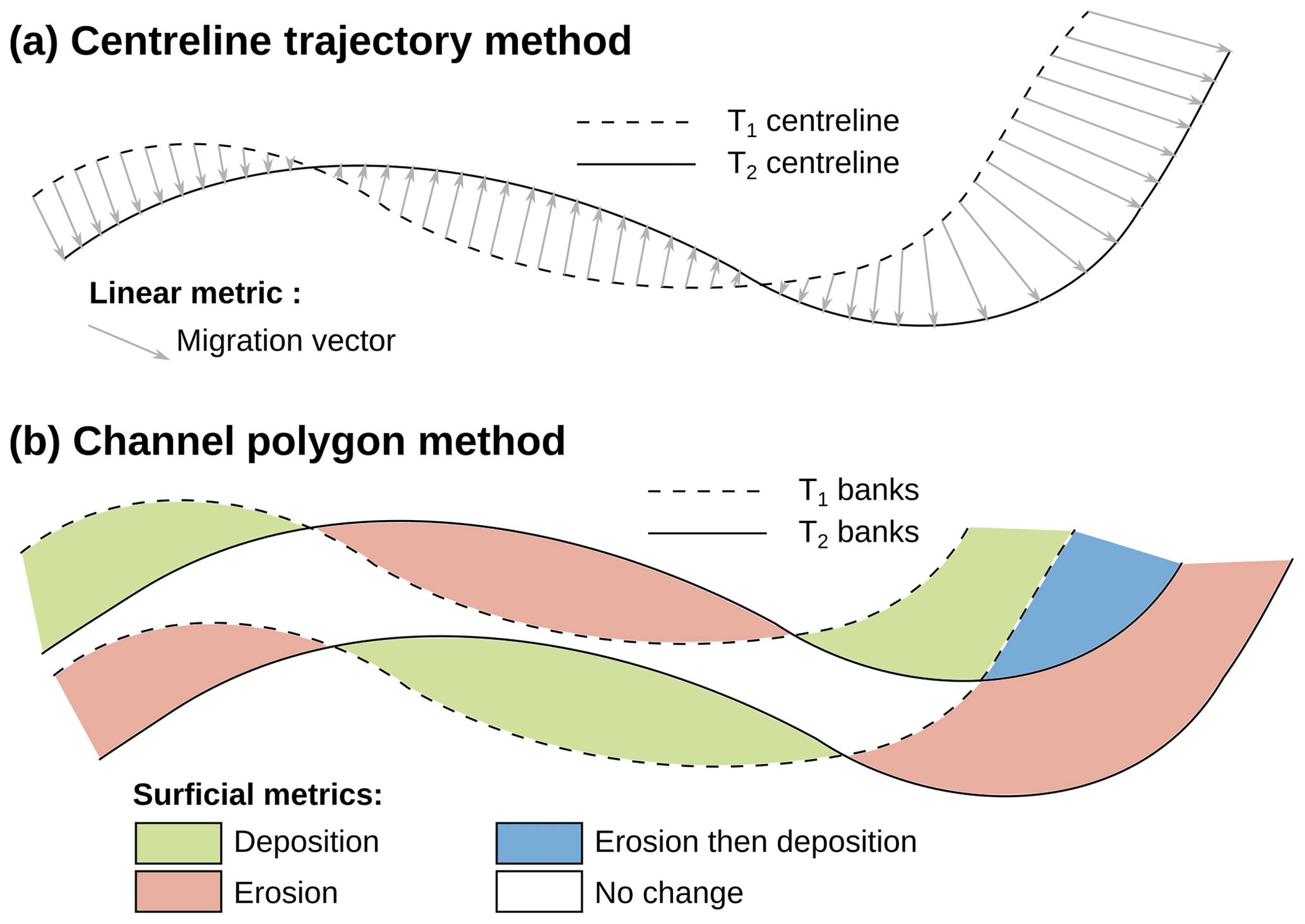
Figure 1Illustration of the lateral migration metric used (a) by Lea and Legleiter (2016) and Donovan et al. (2019) and (b) in this study.
This study aims to advance the generalisation of SV error assessment methods in fluvial settings by testing its impact on the quantification of lateral migration using a surficial metric: the channel polygon method (Fig. 1b). This consists in the extraction of eroded, deposited, and eroded-then-deposited surfaces from overlaid diachronic channels. SV error is assessed in two diachronic orthophotos of the lower Bruche (i.e. a mid-sized tributary of the Rhine), by spatial interpolation (Lea and Legleiter, 2016) based on an independent set of ground control points (Hughes et al., 2006). The main novelty of our approach is running Monte Carlo (MC) simulations (Metropolis and Ulam, 1949) to propagate the geometric error in measurements of eroded and/or deposited surfaces. This eventually allows computing the uncertainty associated with surficial changes, to which a threshold is applied to detect non-significant planform changes.
More specifically, this study tests three hypotheses in the fluvial context: (1) orthophotos are affected by a locally significant SV error; (2) SV error greatly affects the variability of MC-simulated measurements of eroded and/or deposited surfaces; and (3) the uncertainty of surficial changes depends on their magnitude. This work also evaluates the effectiveness of MC simulations in measuring fluvially eroded and/or deposited surfaces and assessing their significance.
Located in easternmost France (Alsace), the Bruche is a mid-sized tributary of the Rhine with a drainage area of about 730 km2. The 80 km long river firstly drains the eastern flank of the Vosges Massif before debouching into the Upper Rhine Graben (Fig. 2a). Although highly impacted by human activities (levee/canal construction, channelisation, and artificial cut-offs), this alluvial river is known to have been laterally active over historical times (Maire, 1966; Payraudeau et al., 2010; Schmitt et al., 2007). This is especially true in its lowermost reach where it flows through the Strasbourg urban area (Fig. 2a), raising important management issues (Payraudeau et al., 2008; Skupinski et al., 2009). Our test site is a 6 km long wandering reach located a few kilometres upstream of the Ill confluence: the river freely meanders within its Holocene floodplain and locally erodes Late Pleistocene terrace deposits of the lower Bruche about 2 km from its confluence as well (Fig. 2a; Maire, 1966). In this reach, the Bruche has a 20 m wide mean active channel and a mean slope of 1 ‰. The daily 2-year (Q2) and 10-year (Q10) peak flow discharges amount to 71 and 126 m3 s−1, respectively, for the period 1965–2018. The specific stream power at the Q2 discharge roughly amounts to 27 W m−2.
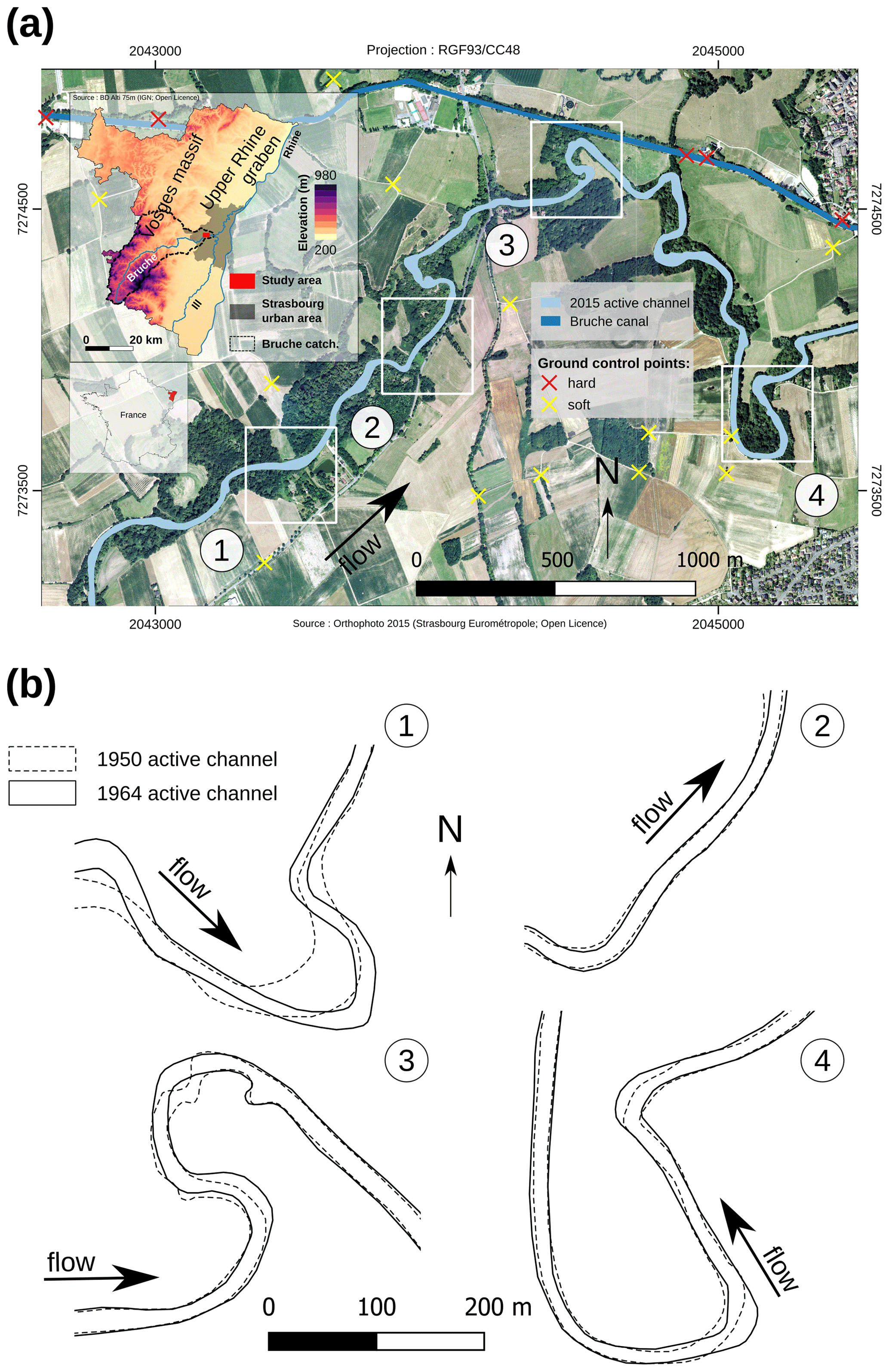
Figure 2(a) Study area. Localisation of the four sub-reaches in the lowermost Bruche course. Red and yellow crosses indicates the position of the independent set of GCPs used to assess the SV error over the study area. (b) Planimetric evolution of each sub-reach from 1950 to 1964 based on the two orthophotos.
3.1 Remotely sensed data
To measure eroded and/or deposited surfaces in our study area, two orthophotos from 1950 and 1964 were used. They were produced by the French National Geographic Institute (IGN) and the Laboratoire Image, Ville, Environnement (LIVE) of the University of Strasbourg; they have a spatial resolution of 50 and 20 cm, respectively. Both are projected in RGF93/CC48 CRS (EPSG: 3948), which is the most accurate projection in this area. Despite the lack of hydrological data in the lower Bruche before 1965, we assume surveys were conducted during moderate to low water, according to the period of the year during which the photos were taken (13 September 1950 and 17 April 1964) and our inspection of the orthophotos.
Active channel is a widely used concept to objectively identify channel boundaries in aerial photographs, regardless of the river discharge. It basically refers to the unvegetated area (Liébault and Piégay, 2001; Liro, 2015; Mandarino et al., 2019; Surian et al., 2009; Winterbottom, 2000). Here, active channel boundaries have been digitised by a single user in QGIS at a 1∕300 scale. To reliably assess the SV error, we used a 2015 orthophoto as the base image; it was produced by the IGN with a resolution of 20 cm.
3.2 SV error assessment
In both orthophotos (1950 and 1964) of our study area, spatial variations of geometric error are assessed by an approach similar to that used by Lea and Legleiter (2016). However, because we use orthophotos (which are already co-registered), we must rely on an independent set of ground control points (GCPs), as suggested by Hughes et al. (2006). We selected a total of 18 GCPs, including both hard (buildings and canal) and soft (pathway intersections and trees) features (Fig. 2a). After identification and manual plotting in the 2015 orthophoto, they are identified in both older orthophotos on a 1∕200 computer-screen scale. The spatial distribution of GCPs in the study area is rather uniform, though hard edges are restricted to the northern sector (Fig. 2a).
Local root square error (RSE) is then measured for each of the 18 GCPs, in both orthophotos. Error in x or y corresponds to the Euclidean distance between the two points for x and y coordinates, respectively. SV error is calculated by interpolating local RSE in our whole study area with an inverse-distance weighting (IDW) technique at the original spatial resolution (Fig. 4). IDW uses a linear combination of values at specific sampled points. It allocated weights proportional to the proximity of the sampled points to estimate values at unknown locations (Ikechukwu et al., 2017). We used the IDW interpolation method for two main reasons. First, based on a comparison of five interpolation methods, Lea and Legleiter (2016) showed that linear and nearest-neighbour methods reduce the areal extent of large co-registration errors. These methods are thus discarded as they can strongly limit the influence of large co-registrations errors in the estimation of surficial changes. Then, in a comparative study of spatial interpolation methods for producing a digital elevation model from a small set of points that were not spatially uniform, Tan and Xu (2014) showed that IDW provided better results than spline or kriging. Because of the difficulties of selecting a high number of independent control points spatially uniform over time in archival remotely sensed data, we argue that IDW is a reliable method for interpolating the registration error in our case.
3.3 Sub-reaches
To examine the implications of SV error in lateral migration measurements, we focus on four distinct sub-reaches (Fig. 2). Their mean thalweg lengths amount to 530, 380, 700, and 890 m long (upstream–downstream order). They are (1) an extending and narrowing meander, (2) an almost straight (apparently inactive) sector, (3) two alternate meanders (the first one slightly extending and the second one displaying a small cut-off), and (4) a long meander extending at the downstream end of the curve. We selected geomorphologically distinct sub-reaches to evaluate the effect of both different magnitude changes and types of geomorphic processes.
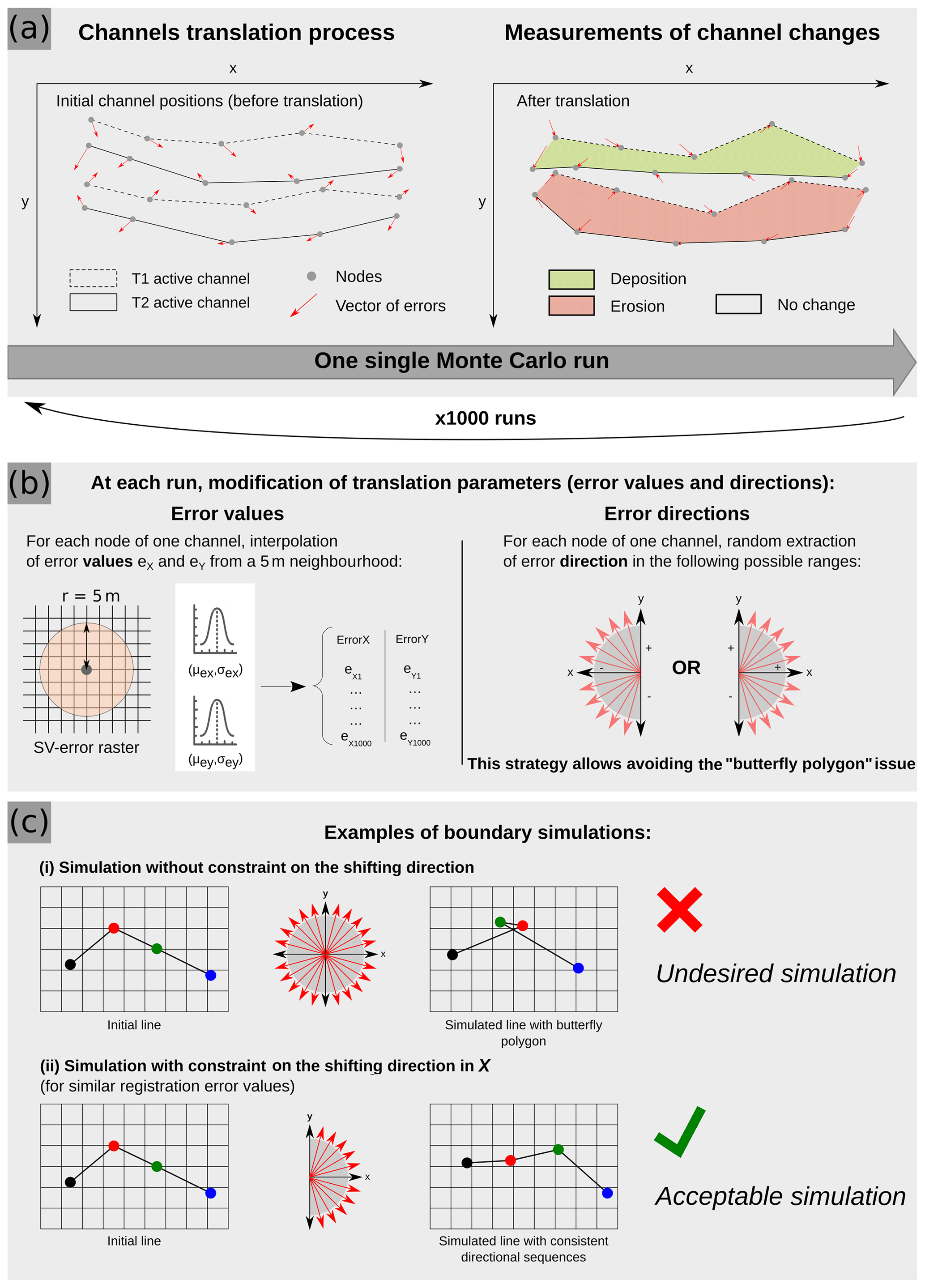
Figure 3Workflow of the Monte Carlo translation process used in this study. (a) Measurements of channel changes after translation. (b) Translation parameters (error values and directions). (c) Illustration of resulting boundary simulations with and without constraints on the shifting direction.
3.4 MC simulations
3.4.1 Channel boundary simulation method
MC simulations as statistical methods are generally used in cases where processes are random or when assumptions in the theoretical mathematics are not well known (Brown and Duh, 2004; Openshaw et al., 1991). Applying MC simulations in this research context is the main novelty of this study. This approach has two main advantages. Firstly, MC simulations are particularly well suited to our problem because of the difficulty of distinguishing between inherent and processing errors in the measured RSE over the whole area. Secondly, MC simulations assume a spatial continuity and a relative spatial homogeneity of the error, which is consistent with resulting spatial patterns of errors observed after the co-registration or digitising process. MC simulations are also relatively easy to perform and applicable in very different cases. This approach could thus improve the generalisation of methods for calculating planform changes and spatially variable uncertainty in a fluvial context, as suggested by Donovan et al. (2019).
The approach used in this study followed the rules of boundary simulations (Burrough et al., 2015). Figure 3 illustrates this part of our methodology. As described in the previous section, SV error has been interpolated over the whole study area. For each channel node, all pixels in a 5 m buffer were first selected. A check of the local distributions of error (Shapiro test) showed a normal distribution for a vast majority of them. The normal distribution of error was then calculated by averaging the mean local error and by calculating the standard deviation for each node, in each sub-reach. Hence, for each run (1000 runs in total), a specific value of error in x () and y () was randomly extracted from the respective normal distribution (Fig. 3b) in order to shift each node from its original position.
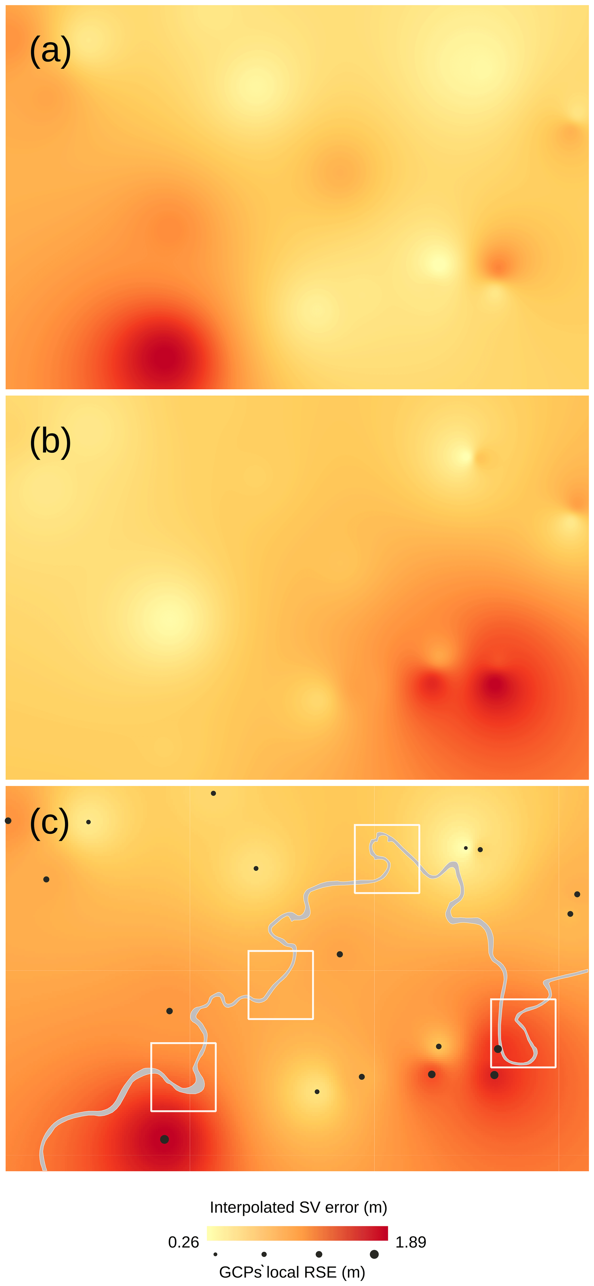
Figure 4SV error interpolation between GCPs from local RSEs, by the IDW method. Year 1950. (a) Error in x. (b) Error in y. (c) Total error.
Furthermore, in accordance with the results from Podobnikar (2008), the shape of a particular channel is assumed to remain coherent after simulation. In this study, as the distance between nodes is significantly higher than the local registration error, it is possible to move nodes of each sub-reach in any x and y direction without significantly impacting the shape. However, when the condition above is violated (in historical maps for instance; see Herrault et al., 2013), the operation can potentially lead to strong geometrical errors such as “butterfly polygons” or excessive geometric distortions (Fig. 3c). These errors might be partially corrected (e.g. via a moving average algorithm or Douglas–Peucker filtering) but can result in erroneous modifications of the original channel shape. Thus, we proposed a hybrid solution to simulate the node shifting in space: (1) nodes from one sub-reach can move in any y direction (i.e. positive or negative) at each run, and (2) nodes from one sub-reach can move in only one x direction at each run (Fig. 3b). Considering the strong correlation of registration errors between two successive points, constraining the shifting direction for one of the two coordinates allows maintaining the directional sequence of several successive nodes and avoiding the butterfly polygon issue. From a wider perspective, the last operation allows (i) avoiding topological errors (Fig. 3c) while simulating the most probable displacements of channel polygons and (ii) probably enhancing the transferability of our method to other fluvial settings. The direction of errors in x and y were randomly selected at each MC simulation with equal probability weights (i.e. 50 % each).
Last, as mentioned by Donovan et al. (2019), it is quite hard to distinguish between errors inherent to the co-registration and digitising processes. For this reason, a digitising error (ed) equal to 1 pixel was added as a reasonable constraint within the simulation process, considering the resolution of the orthophotos. This digitising error is assumed to be uniform over the entire area and does not fluctuate in different simulation runs (Eqs. 1 and 2). Only the direction in x and y was randomly defined for each node of one sub-reach at each MC simulation. These directions may vary from one node to another for one given sub-reach.
The overall mathematical expression of the simulation process can be expressed as follows:
where and are the absolute registration error in x and y, respectively. The constant ed is the digitising error equal to 1 pixel. β1 and β2 respectively are the coefficients of shifting direction (i.e. 1 or −1) of the registration error (i.e. and ) and the digitising error (ed), randomly selected at each run. In our study, β1 was constant for each xchanged of one sub-reach (i.e. constrained in only one direction).
3.4.2 Lateral migration measurements
Lateral migration of the river channel between 1950 and 1964 is calculated through three standard surficial morphological metrics (erosion, deposition, and erosion then deposition), illustrated in Fig. 1b. Note that the metric “erosion then deposition” measured in the area located between the former channel (T1) and the new one (T2) does not always imply continuous lateral channel migration followed by deposition. Sudden lateral shifts of meanders (e.g. through meander cut-off) or meander belts (e.g. through channel avulsion) may be involved as well and require specific geomorphological attention. Therefore, at each MC run, new values of metrics are derived for each sub-reach (Fig. 3a) in order to estimate fluctuations induced by co-registration and digitising errors.
3.4.3 Impact of SV error on uncertainty of lateral migration measurements
To evaluate the uncertainty associated with lateral migration measurements within each sub-reach and to allow comparison between the four sub-reaches, two types of relative uncertainty were calculated for each morphological metric (erosion, deposition, and erosion then deposition). The first one (Eq. 3) corresponds to the total percentage of uncertainty and involves the total range of measured values (max–min) through MC simulation. The second one (Eq. 4) corresponds to the 95 % uncertainty percentage and involves the 95 % confidence interval. Their mathematical expressions are, respectively,
Relative percentages of uncertainty provide information about the variability of measurements induced by the SV error through MC simulation, observed in each sub-reach and for each morphological metric. We thus use these relative percentages of uncertainty to set a threshold of 50 %, above which the uncertainty is considered too high to yield a reliable measurement, i.e. a significant change in channel migration. It is proposed to apply the 50 % threshold to both percentages of uncertainty: the less conservative one (i.e. 95 % uncertainty >50 %) and the more conservative one (i.e. total uncertainty >50 %). While the former does not include outliers, the latter, which corresponds to a measurement whose mean value is lower than the total range of measured values (max–min), does. In other words, applying the proposed 50 % threshold to the total uncertainty amounts to assuming that outliers can be “real” (i.e. that they can represent plausible situations). By contrast, applying the proposed 50 % threshold to the 95 % uncertainty amounts to rejecting the outliers, assuming that they cannot be real (implausible situations).
4.1 SV error
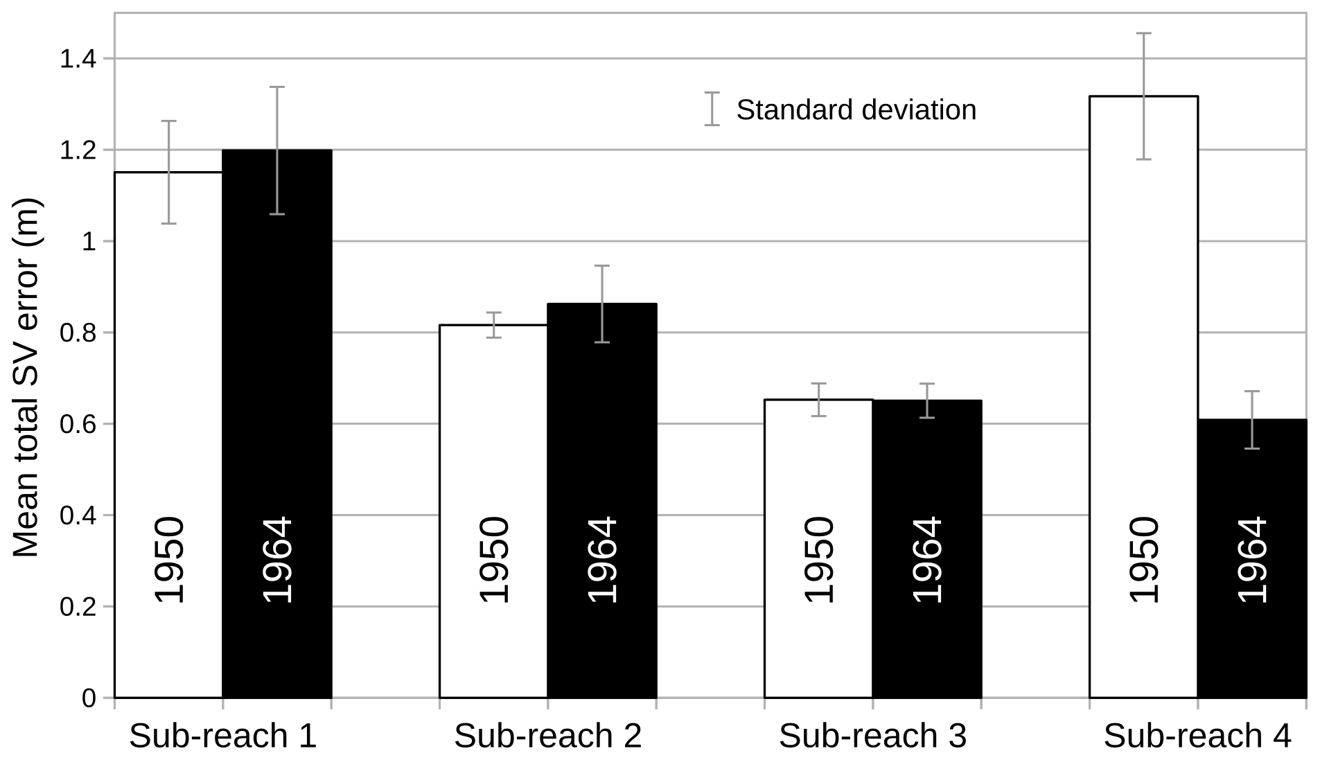
Figure 4 shows the interpolated SV error in x and y, and the total SV error () for the year 1950. The mean value of total SV error in each sub-reach for both years (Fig. 5) indicates that sub-reach 4 is affected by the highest (1.32 m) and the lowest (0.61 m) error in 1950 and in 1964, respectively. These values approximately correspond to the range of total SV error reached by the four sub-reaches. Whereas the total SV error was reduced by a factor of 2 between 1950 and 1964 in sub-reach 4, it remained fairly stable in the three other ones, ranging from 0.6 (sub-reach 3) to 1.2 m (sub-reach 1).
4.2 MC simulations
An example of variations in measurements of eroded surface through MC simulations is presented for sub-reach 1 in Fig. 6. The entirety of MC results are available in Appendix A. A large majority of the measurements appear to be randomly varying around and close to the mean value, inside the 95 % confidence interval. Note that having few outliers sometimes greatly extends the maximum range compared to the 95 % confidence interval, especially when very low values occur. For instance, MC simulations for deposited surfaces in sub-reach 1 include an outlier with a value (2.5×10³ m2) corresponding to 38 % of the mean measured value (6.8×10³ m2).
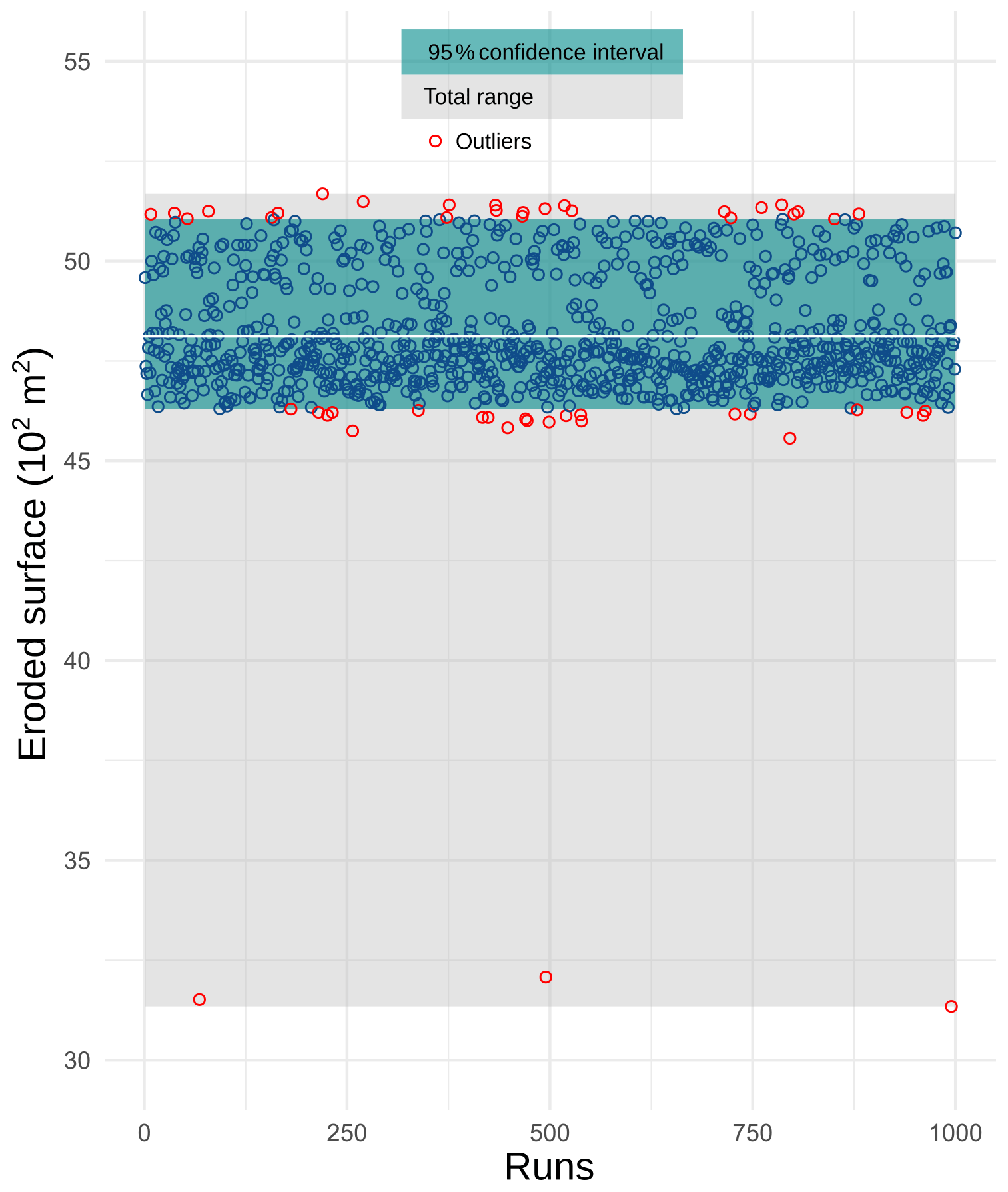
Figure 6Measurements of eroded surface in sub-reach 1, through 1000 MC simulations. Grey horizontal line corresponds to the mean value.
Mean changes inferred from MC simulations between 1950 and 1964 are presented in Fig. 7a. Comparison between sub-reaches is allowed by the normalisation of the surficial changes by the respective thalweg lengths of each sub-reach (expressed thus in m2 m−1). Whatever the sub-reach, changes in eroded or deposited surfaces are much larger than those associated with erosion/deposition. The latter are either negligible (sub-reaches 1 and 3) or not recorded (sub-reaches 2 and 4). Sub-reach 1 shows the largest migration: eroded and deposited surfaces amount to and , respectively. By contrast, sub-reach 2 shows the lowest migration: eroded and deposited surfaces amount to and , respectively. Intermediate measurements are reported in sub-reaches 3 and 4, where they range between (deposition; sub-reach 4) and (erosion; sub-reach 4). Note that, in these two last sub-reaches, changes in eroded surfaces are at least twice as high as those in deposited surfaces.
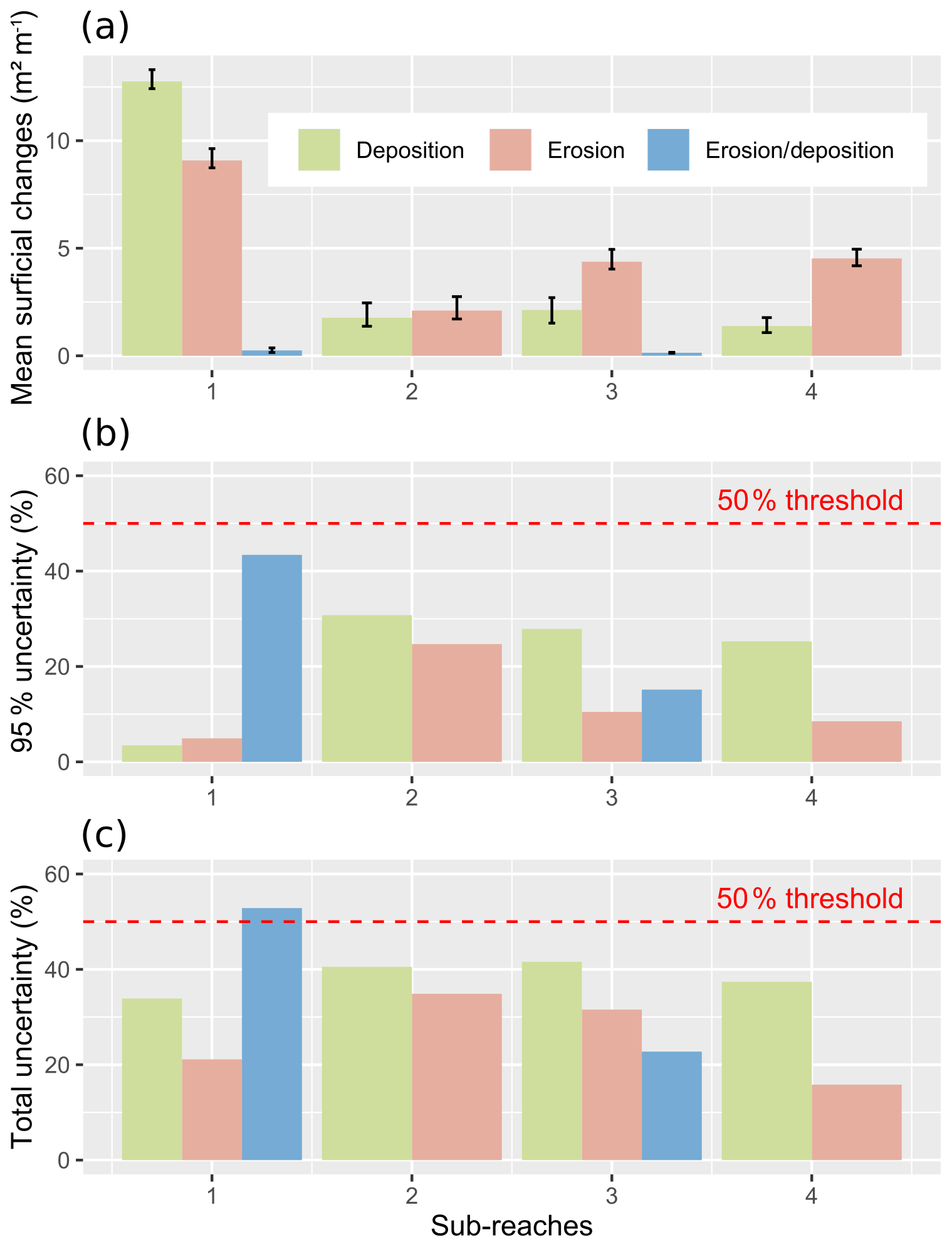
Figure 7(a) Mean surficial changes normalised by the length of each sub-reach. Error bars correspond to the 95 % confidence interval. (b) 95 % uncertainty percentage (without outliers). (c) Total uncertainty percentage (with outliers). The red dashed line corresponds to the 50 % proposed threshold.
4.3 Uncertainty in lateral migration measurements
The relative percentage of measurement uncertainty in surficial changes is presented both in the 95 % confidence interval (95 % uncertainty; Eq. (4); Fig. 7b) and in the whole range of measured values (total uncertainty; Eq. (3); Fig. 7c). As a reminder, the 95 % uncertainty does not take into account the presence of outliers, while the total uncertainty does. The 95 % uncertainty varies from 3.5 % to 43.4 %. These extreme values both occur in sub-reach 1, for the deposited and the eroded-then-deposited surfaces, respectively. The total uncertainty varies from 15.8 % to 52.9 %. These extreme values both occur in sub-reach 4 and 1, for the eroded and the eroded-then-deposited surfaces, respectively. Sub-reaches 2 and 4 both display the same pattern between the 95 % and the total uncertainty, with the uncertainty related to the deposited surface being higher than that related to the eroded one. In contrast, sub-reaches 1 and 3 do not display the same pattern between the 95 % and the total uncertainty. For sub-reach 1 and relative to the uncertainty of the eroded surface, the uncertainty of the deposited surface is higher than the latter only when taking into account the presence of outliers (total uncertainty). For sub-reach 3 and relative to the uncertainty of the eroded/deposited surface, the uncertainty of the eroded surface is higher than the latter only when taking into account the presence of outliers (total uncertainty).
In the light of these new results, we first discuss the three hypotheses underlying this study. In the second step, we propose some methodological guidelines together with promising further implications of this study.
5.1 SV error implications for uncertainty of surficial planform changes
Our results support the first hypothesis: they confirm that orthophotos are affected by a local significant SV error. Within our relatively small (∼6 km2) and flat study area, we interpolated a total SV error ranging from 0.26 to 1.89 m (Fig. 4), while mean values of total SV error range from 0.61 to 1.32 m for the four sub-reaches (Fig. 5). This emphasises the need to take the SV error into account and, importantly, to assess its impact on the uncertainty of the measured changes (Lea and Legleiter, 2016; Donovan et al., 2019), even if the characteristics of the studied reach may appear unproblematic at first glance. Moreover, as orthophotos are used in this study, we draw particular attention to the relevance of this statement in the case of studies using co-registered aerial photographs for similar purposes (e.g. Cadol et al., 2010; Hooke and Yorke, 2010; Sanchis-Ibor et al., 2019).
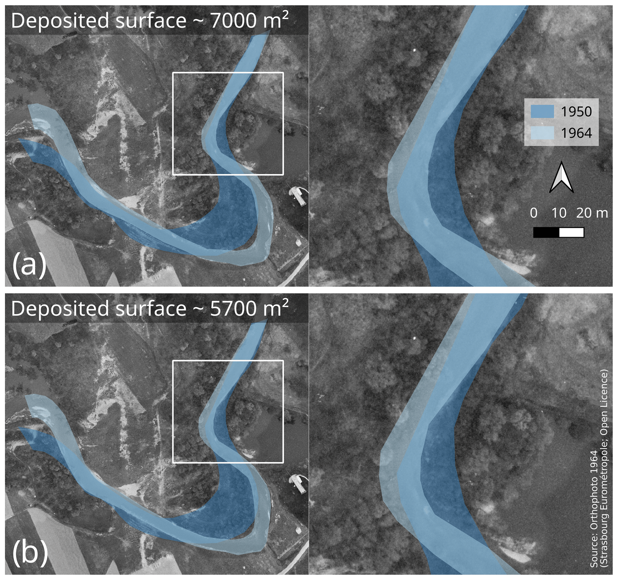
Figure 8Example of translated channels for sub-reach 1, resulting from two different MC runs. Distinction between an (a) inlier and an (b) outlier according to the simulated deposited surface. Background corresponds to the 1964 orthophoto.
Our results also support the second hypothesis: the SV error greatly affects the variability of MC-simulated measurements of eroded and/or deposited surfaces. Variability of the surficial measurements has been assessed by calculating the relative percentages of uncertainty induced by the SV error through the MC simulations. Whereas the more conservative percentage of uncertainty (total uncertainty) ranges from 15.8 % to 52.9 %, depending on the metric and the sub-reach, the less conservative percentage of uncertainty (95 % uncertainty) still ranges from 3.5 % to 43.4 %. These results highlight the potentially high impact that SV error can have on variability of surficial measurements and consequently on their uncertainty.
When applying the more conservative threshold of significance (50 % of total uncertainty; cf Sect. 3.4.3), it appears that only one surficial change has to be considered non-significant (eroded/deposited surface in sub-reach 1; Fig. 7c). However, it can be considered significant when applying the less conservative threshold of significance (Fig. 7b), because its uncertainty does not reach the 50 % threshold. While this contrast may call into question whether or not the presence of outliers should be taken into account, visual comparison of specific situations may help to unravel this issue. As illustrated in Fig. 8, only subtle areal and shape differences may be observed between an inlier and an outlier, the latter likely representing a geomorphologically plausible situation. When using MC simulations in this context, we thus strongly suggest inspecting outliers and not systematically rejecting them. When the geomorphological plausibility of outliers is doubtful, we recommend using the total percentage of uncertainty.
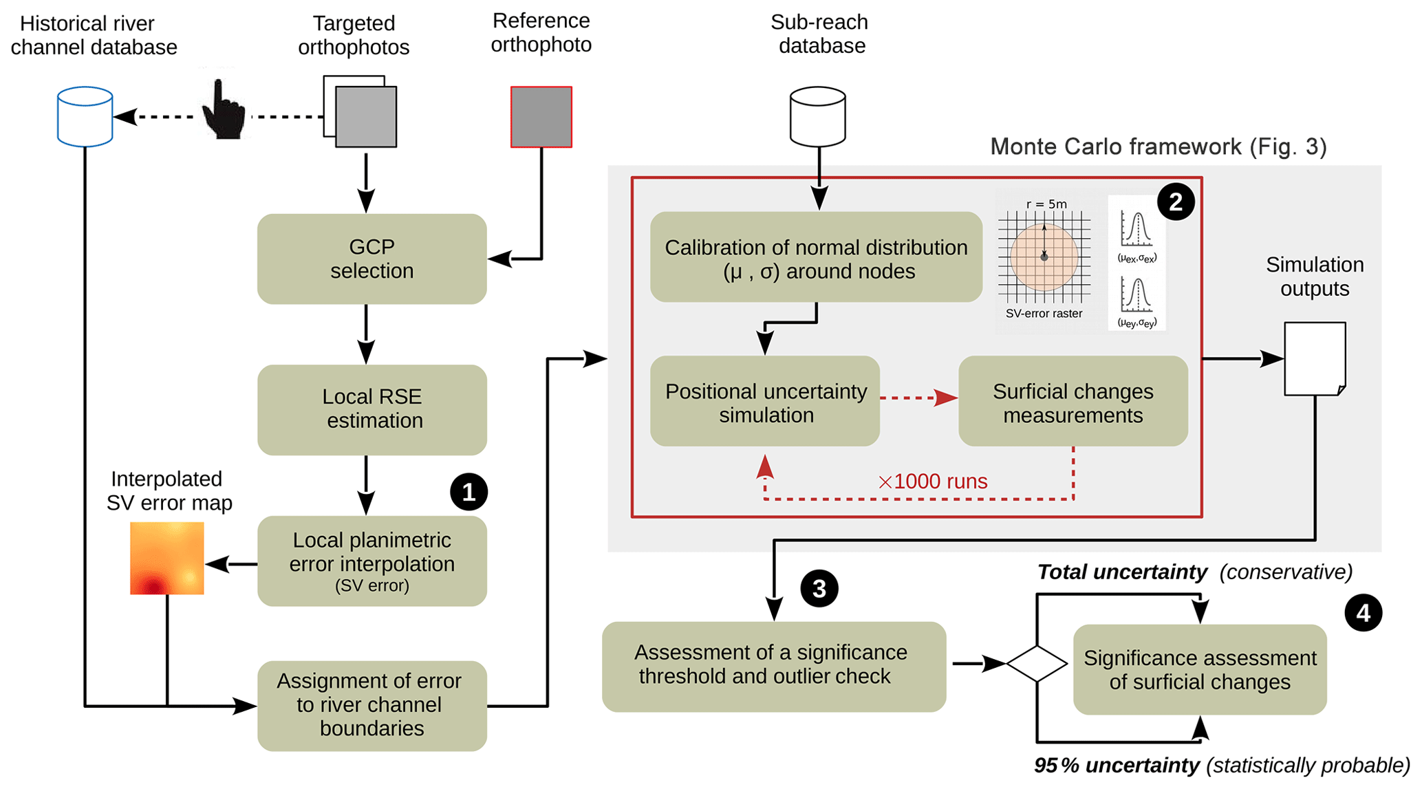
Figure 9Detailed flow chart of the methodology applied in this study, allowing uncertainty of eroded and/or deposited surfaces to be assessed using SV error.
Our results partly validate the third hypothesis: the uncertainty of surficial changes depends not only on their magnitude but also possibly on their respective shapes. A contrasted pattern of uncertainty is observed in sub-reaches 2 and 4 versus sub-reaches 1 and 3. Whereas the former seemingly display uncertainties solely related to the magnitude of changes (i.e. higher uncertainties for lower surficial changes), the latter do not (i.e. in some cases, higher uncertainties for higher surficial changes; see Sect. 4.3). It is the case for instance in sub-reach 3, which displays a higher total uncertainty for the eroded surface than for the eroded-then-deposited surface. Yet, as sub-reaches 1 and 3 display more complex geomorphological shapes and channel evolution than sub-reaches 2 and 4 (Fig. 2b), we suggest that uncertainty of surficial measurements might also be strongly influenced by channel morphology and its evolution through time.
5.2 Methodological guidelines and potential applications
In order to improve the generalisation of tools documenting fluvial planform changes and facilitate the implementation of our new methodological framework, we can summarise the complete workflow as follows (see Fig. 9 for more details): (1) interpolate the SV error in the study area (as recommended in Lea and Legleiter, 2016), (2) calibrate a normal distribution around nodes to randomly translate these (see Fig. 3 for more details), (3) choose a significance threshold, and visually check the outliers to eventually (4) assess the significance of the measured surficial planform changes. The key step (2) is achieved via MC simulation, which is well known for its simplicity, reliability, and transferability (Brown and Duh, 2004; Openshaw et al., 1991). Simulation outputs allow assessing both the total and the 95 % uncertainties (Fig. 9).
We suggest a few practical recommendations when applying the proposed methodological framework. If orthophotos are employed, we strongly advise using an independent set of GCPs for co-registration, bearing in mind that orthophotos are affected by a significant SV error (see Sect. 5.1). As for GCPs, their amount must be high enough and their distribution over the entire study area as homogeneous as possible. As pointed out by Hughes et al. (2006), a location of these GCPs close to the river system is highly beneficial. As for the 50 % significance threshold, we recommend applying it in the total uncertainty, as outliers might represent geomorphologically plausible situations (Fig. 8). Nevertheless, the few outliers (Fig. 6) should still be treated in an empirical manner by visually determining if they should be rejected or not. Further work is required in the near future to deal with this issue in a more automatic way. More generally, when studying historical lateral migration of mid-sized rivers (active channel width <30 m) and/or low-magnitude changes (<1 ) with the channel polygon method, we emphasise the systematic need for assessing both SV error and uncertainty, as some of the measured changes might be non-significant (see Sect. 5.1).
This study, though focusing on short sub-reaches of a mid-sized (∼20 m) meandering (single-thread) channel using specific remotely sensed data on a short timescale (archival orthophotos), has great potential for transferability. Firstly, we assume that our methodological framework could be applied to any fluvial system, regardless of its size. Secondly, we likewise argue that it could be relatively easily extended onto an entire river reach by increasing the sub-reach database and/or onto a longer temporal scale by increasing the historical river channel database (Fig. 9). As for the size/length of the sub-reaches, we recommend adapting it according to the complexity of the planform changes and/or the channel pattern (e.g. anastomosing and anabranching channel patterns). As for the river channel database, other remotely sensed data, such as co-registered aerial photographs and satellite imagery, or traditional planimetric data (maps) can be easily integrated as well. Thirdly, transferring this framework to other channel patterns represents a promising future research topic. In contrast to the centreline approach (e.g. Lea and Legleiter, 2016), the channel polygon method would actually suit the study of lateral mobility of multi-threaded channels (including anastomosing rivers, which usually are characterised by low lateral mobility), with a robust assessment of the SV error. Unlike this present study, where planimetric changes associated with erosion/deposition are negligible, we might expect a higher proportion of these changes in this kind of fluvial setting. Overall, long-term landscape reconstruction studies could also greatly benefit from the methodology we propose. In particular, works combining multiple diachronic spatial sources (e.g. old aerial photographs, historical and cadastre maps, and satellite images) should draw particular attention because of the possible propagation of uncertainty in the assessment of landscape changes.
We conclude by stating that this study offers promising research prospects. Firstly, a key outcome is the ability of MC simulations to actually detect low-magnitude planform changes in mid-sized river channels. This positive achievement thus overcomes the main difficulty related to the use of classic planimetric methods in such settings (Piégay et al., 2005), as recently highlighted by Lauer et al. (2017), who failed to detect noticeable changes in mid-sized active channels (width < 25 m). Secondly, as for river restoration, our methodological framework should help in constructing robust scenarios of future river management, especially those based on past planform changes (e.g. Marçal et al., 2017). Thirdly, significance assessment of planform changes can strengthen the studies using surfaces of an active channel as input for sediment budgeting (Wheaton et al., 2009). Finally, while this study, together with Lea and Legleiter (2016) and Donovan et al. (2019), focus specifically on the SV error and, more globally, uncertainties in planimetric studies in a wide range of fluvial settings, the proposed propagation of geometric error via MC simulations could be extended to other geomorphological contexts where surface extraction from remotely sensed data is involved.

Datasets and code are available upon request from Timothée Jautzy (timothee.jautzy2@etu.unistra.fr).
All authors contributed to the conception of this study and manuscript writing. TJ wrote most of the manuscript and produced the initial data and figures; TJ and PAH conceptualised the global processing chain and performed Monte Carlo simulations; VC contributed to result interpretation; LS and GR provided a complete review of the manuscript; and GR supervised the text harmonisation.
The authors declare that they have no conflict of interest.
We warmly thank Grégoire Skupinski (LIVE) for providing orthophotos. We are grateful to Josué Jautzy (Geological Survey of Canada) for his valuable review of the first draft. We also thank two anonymous reviewers, who helped to significantly improve this paper. This work has been entirely produced with free and open-source programs (QGIS, R, GDAL, Inkscape, LibreOffice, and LaTeX).
This research has been supported by the Scientific Council of the National School for Water and Environmental Engineering of Strasbourg (ENGEES, France; grant no. 6803MOBI).
This paper was edited by Francois Metivier and reviewed by two anonymous referees.
Biron, P. M., Buffin-Bélanger, T., Larocque, M., Choné, G., Cloutier, C.-A., Ouellet, M.-A., Demers, S., Olsen, T., Desjarlais, C., and Eyquem, J.: Freedom Space for Rivers: A Sustainable Management Approach to Enhance River Resilience, Environ. Manage., 54, 1056–1073, https://doi.org/10.1007/s00267-014-0366-z, 2014. a
Bollati, I., Pellegrini, L., Rinaldi, M., Duci, G., and Pelfini, M.: Reach-scale morphological adjustments and stages of channel evolution: The case of the Trebbia River (northern Italy), Geomorphology, 221, 176–186, https://doi.org/10.1016/j.geomorph.2014.06.007, 2014. a
Brown, D. G. and Duh, J.-D.: Spatial simulation for translating from land use to land cover, Int. J. Geogr. Inf. Sci., 18, 35–60, https://doi.org/10.1080/13658810310001620906, 2004. a, b
Burrough, P. A., McDonnell, R., McDonnell, R. A., and Lloyd, C. D.: Principles of geographical information systems, Oxford University Press, 2015. a
Cadol, D., Rathburn, S. L., and Cooper, D. J.: Aerial photographic analysis of channel narrowing and vegetation expansion in Canyon De Chelly National Monument, Arizona, USA, 1935–2004, River Res. Appl., 27, 841–856, https://doi.org/10.1002/rra.1399, 2010. a, b
Comiti, F., Da Canal, M., Surian, N., Mao, L., Picco, L., and Lenzi, M.: Channel adjustments and vegetation cover dynamics in a large gravel bed river over the last 200 years, Geomorphology, 125, 147–159, https://doi.org/10.1016/j.geomorph.2010.09.011, 2011. a
De Rose, R. C. and Basher, L. R.: Measurement of river bank and cliff erosion from sequential LIDAR and historical aerial photography, Geomorphology, 126, 132–147, https://doi.org/10.1016/j.geomorph.2010.10.037, 2011. a
Donovan, M., Miller, A., Baker, M., and Gellis, A.: Sediment contributions from floodplains and legacy sediments to Piedmont streams of Baltimore County, Maryland, Geomorphology, 235, 88–105, https://doi.org/10.1016/j.geomorph.2015.01.025, 2015. a
Donovan, M., Belmont, P., Notebaert, B., Coombs, T., Larson, P., and Souffront, M.: Accounting for uncertainty in remotely-sensed measurements of river planform change, Earth-Sci. Rev., 193, 220–236, https://doi.org/10.1016/j.earscirev.2019.04.009, 2019. a, b, c, d, e, f, g, h, i
Downward, S., Gurnell, A., and Brookes, A.: A methodology for quantifying river channel planform change using GIS, IAHS Publications-Series of Proceedings and Reports-Intern. Assoc. Hydrological Sciences, 224, 449–456, 1994. a
EPCEU: Directive 2000/60/EC of the European parliament and of the council of 23 October 2000 establishing a framework for Community action in the field of water policy, Official Journal of the European Communities, 72 pp., available at: https://ec.europa.eu/health/sites/health/files/endocrine_disruptors/docs/wfd_200060ec_directive_en.pdf (last access: 14 February 2020), 2000. a, b
Gaeuman, D., Symanzik, J., and Schmidt, J. C.: A Map Overlay Error Model Based on Boundary Geometry, Geogr. Anal., 37, 350–369, https://doi.org/10.1111/j.1538-4632.2005.00585.x, 2005. a
Güneralp, Ä., Filippi, A. M., and Hales, B.: Influence of river channel morphology and bank characteristics on water surface boundary delineation using high-resolution passive remote sensing and template matching: river water delineation using remote sensing and template matching, Earth Surf. Proc. Land., 39, 977–986, https://doi.org/10.1002/esp.3560, 2014. a
Gurnell, A. M., Downward, S. R., and Jones, R.: Channel planform change on the River Dee meanders, 1876–1992, Regul. River., 9, 187–204, https://doi.org/10.1002/rrr.3450090402, 1994. a, b, c
Hajdukiewicz, H. and Wyżga, B.: Aerial photo-based analysis of the hydromorphological changes of a mountain river over the last six decades: The Czarny Dunajec, Polish Carpathians, Sci. Total Environ., 648, 1598–1613, https://doi.org/10.1016/j.scitotenv.2018.08.234, 2019. a
Herrault, P.-A., Sheeren, D., Fauvel, M., Monteil, C., and Paegelow, M.: A comparative study of geometric transformation models for the historical “Map of France” registration, Geographia Technica, 8, 34–46, 2013. a
Hooke, J. M. and Yorke, L.: Rates, distributions and mechanisms of change in meander morphology over decadal timescales, River Dane, UK, Earth Surf. Proc. Land., 35, 1601–1614, https://doi.org/10.1002/esp.2079, 2010. a, b, c
Hughes, M. L., McDowell, P. F., and Marcus, W. A.: Accuracy assessment of georectified aerial photographs: implications for measuring lateral channel movement in a GIS, Geomorphology, 74, 1–16, 2006. a, b, c, d
Ikechukwu, M. N., Ebinne, E., Idorenyin, U., and Raphael, N. I.: Accuracy Assessment and Comparative Analysis of IDW, Spline and Kriging in Spatial Interpolation of Landform (Topography): An Experimental Study, Journal of Geographic Information System, 09, 354–371, https://doi.org/10.4236/jgis.2017.93022, 2017. a
Janes, V. J. J., Nicholas, A. P., Collins, A. L., and Quine, T. A.: Analysis of fundamental physical factors influencing channel bank erosion: results for contrasting catchments in England and Wales, Environ. Earth Sci., 76, 307, https://doi.org/10.1007/s12665-017-6593-x, 2017. a, b
Lauer, J. W. and Parker, G.: Net local removal of floodplain sediment by river meander migration, Geomorphology, 96, 123–149, https://doi.org/10.1016/j.geomorph.2007.08.003, 2008. a
Lauer, J. W., Echterling, C., Lenhart, C., Belmont, P., and Rausch, R.: Air-photo based change in channel width in the Minnesota River basin: Modes of adjustment and implications for sediment budget, Geomorphology, 297, 170–184, https://doi.org/10.1016/j.geomorph.2017.09.005, 2017. a, b, c, d
Lauer, W.: NCED Stream Restoration Toolbox-Channel Planform Statistics And ArcMap Project, National Center for Earth-Surface Dynamics (NCED), available at: https://repository.nced.umn.edu/browser.php?current=keyword&keyword=5&dataset_id=15&folder=237802 (last access: 11 November 2019), 2006. a
Lea, D. M. and Legleiter, C. J.: Refining measurements of lateral channel movement from image time series by quantifying spatial variations in registration error, Geomorphology, 258, 11–20, https://doi.org/10.1016/j.geomorph.2016.01.009, 2016. a, b, c, d, e, f, g, h, i, j, k, l
Legleiter, C. J.: Downstream Effects of Recent Reservoir Development on the Morphodynamics of a Meandering Channel: Savery Creek, Wyoming, USA, River Res. Appl., 31, 1328–1343, https://doi.org/10.1002/rra.2824, 2015. a
Liébault, F. and Piégay, H.: Assessment of channel changes due to long-term bedload supply decrease, Roubion River, France, Geomorphology, 36, 167–186, https://doi.org/10.1016/S0169-555X(00)00044-1, 2001. a, b
Liro, M.: Estimation of the impact of the aerialphoto scale and the measurement scale on the error in digitization of a river bank, Z. Geomorphol., 59, 443–453, https://doi.org/10.1127/zfg/2014/0164, 2015. a
Lovric, N. and Tosic, R.: Assessment of Bank Erosion, Accretion and Channel Shifting Using Remote Sensing and GIS: Case Study – Lower Course of the Bosna River, Quaestiones Geographicae, 35, 81–92, https://doi.org/10.1515/quageo-2016-0008, 2016. a
Maire, G.: La Basse-Bruche : cône de piedmont et dynamique actuelle, Ph.D. thesis, Université de Strasbourg, Faculté de géographie et d'aménagement, 1966. a, b
Mandarino, A., Maerker, M., and Firpo, M.: Channel planform changes along the Scrivia River floodplain reach in northwest Italy from 1878 to 2016, Quaternary Res., 91, 620–637, https://doi.org/10.1017/qua.2018.67, 2019. a, b
Marçal, M., Brierley, G., and Lima, R.: Using geomorphic understanding of catchment-scale process relationships to support the management of river futures: Macaé Basin, Brazil, Appl. Geogr., 84, 23–41, https://doi.org/10.1016/j.apgeog.2017.04.008, 2017. a, b
Metropolis, N. and Ulam, S.: The Monte Carlo Method, J. Am. Stat. Assoc., 44, 335–341, https://doi.org/10.1080/01621459.1949.10483310, 1949. a
Micheli, E. R. and Kirchner, J. W.: Effects of wet meadow riparian vegetation on streambank erosion. 2. Measurements of vegetated bank strength and consequences for failure mechanics, Earth Surf. Proc. Land., 27, 687–697, https://doi.org/10.1002/esp.340, 2002. a
Miller, J. R. and Friedman, J. M.: Influence of flow variability on floodplain formation and destruction, Little Missouri River, North Dakota, Geol. Soc. Am. Bull., 121, 752–759, https://doi.org/10.1130/B26355.1, 2009. a
Morais, E. S., Rocha, P. C., and Hooke, J.: Spatiotemporal variations in channel changes caused by cumulative factors in a meandering river: The lower Peixe River, Brazil, Geomorphology, 273, 348–360, https://doi.org/10.1016/j.geomorph.2016.07.026, 2016. a
Mount, N. and Louis, J.: Estimation and propagation of error in measurements of river channel movement from aerial imagery, Earth Surf. Proc. Land., 30, 635–643, https://doi.org/10.1002/esp.1172, 2005. a
Mount, N., Louis, J., Teeuw, R., Zukowskyj, P., and Stott, T.: Estimation of error in bankfull width comparisons from temporally sequenced raw and corrected aerial photographs, Geomorphology, 56, 65–77, https://doi.org/10.1016/S0169-555X(03)00046-1, 2003. a
O'Connor, J. E., Jones, M. A., and Haluska, T. L.: Flood plain and channel dynamics of the Quinault and Queets Rivers, Washington, USA, Geomorphology, 51, 31–59, https://doi.org/10.1016/S0169-555X(02)00324-0, 2003. a, b
Openshaw, S., Charlton, M., and Carver, S.: Error propagation: a Monte Carlo simulation, Handling geographical information, 78–101, 1991. a, b
Payraudeau, S., Glatron, S., Rozan, A., Eleuterio, J., Auzet, A.-V., Weber, C., and Liébault, F.: Inondation en espace péri-urbain: convoquer un éventail de disciplines pour analyser l'aléa et la vulnérabilité de la basse-Bruche (Alsace), in: actes du colloque ≪Vulnérabilités sociétales, risques et environnement. Comprendre et évaluer≫, Université Toulouse – le Mirail, 14, 15 pp., 2008. a
Payraudeau, S., Galliot, N., Liébault, F., and Auzet, A.-V.: Incertitudes associées aux données géographiques pour la quantification des vitesses de migration des méandres-Application à la vallée de la Bruche, Revue Internationale de Géomatique, 20, 221–243, 2010. a, b
Piégay, H., Darby, S. E., Mosselman, E., and Surian, N.: A review of techniques available for delimiting the erodible river corridor: a sustainable approach to managing bank erosion, River Res. Appl., 21, 773–789, https://doi.org/10.1002/rra.881, 2005. a, b
Podobnikar, T.: Simulation and Representation of the Positional Errors of Boundary and Interior Regions in Maps, in: Geospatial Vision, edited by: Moore, A. and Drecki, I., Springer Berlin Heidelberg, Berlin, Heidelberg, 141–169, https://doi.org/10.1007/978-3-540-70970-1_7, 2008. a
Rhoades, E. L., O'Neal, M. A., and Pizzuto, J. E.: Quantifying bank erosion on the South River from 1937 to 2005, and its importance in assessing Hg contamination, Appl. Geogr., 29, 125–134, https://doi.org/10.1016/j.apgeog.2008.08.005, 2009. a
Rowland, J. C., Shelef, E., Pope, P. A., Muss, J., Gangodagamage, C., Brumby, S. P., and Wilson, C. J.: A morphology independent methodology for quantifying planview river change and characteristics from remotely sensed imagery, Remote Sens. Environ., 184, 212–228, https://doi.org/10.1016/j.rse.2016.07.005, 2016. a
Sanchis-Ibor, C., Segura-Beltrán, F., and Navarro-Gómez, A.: Channel forms and vegetation adjustment to damming in a Mediterranean gravel-bed river (Serpis River, Spain): Channel and vegetation adjustment to damming in a gravel bed river, River Res. Appl., 35, 37–47, https://doi.org/10.1002/rra.3381, 2019. a, b
Schmitt, L., Maire, G., Nobelis, P., and Humbert, J.: Quantitative morphodynamic typology of rivers: a methodological study based on the French Upper Rhine basin, Earth Surf. Proc. Land., 32, 1726–1746, https://doi.org/10.1002/esp.1596, 2007. a
Schook, D. M., Rathburn, S. L., Friedman, J. M., and Wolf, J. M.: A 184-year record of river meander migration from tree rings, aerial imagery, and cross sections, Geomorphology, 293, 227–239, https://doi.org/10.1016/j.geomorph.2017.06.001, 2017. a
Skupinski, G., BinhTran, D., and Weber, C.: Les images satellites Spot multi-dates et la métrique spatiale dans l'étude du changement urbain et suburbain – Le cas de la basse vallée de la Bruche (Bas-Rhin, France), Cybergeo, Systèmes, Modélisation, Géostatistiques, 439, https://doi.org/10.4000/cybergeo.21995, 2009. a
Surian, N., Mao, L., Giacomin, M., and Ziliani, L.: Morphological effects of different channel-forming discharges in a gravel-bed river, Earth Surf. Proc. Land., 34, 1093–1107, https://doi.org/10.1002/esp.1798, 2009. a, b
Swanson, B. J., Meyer, G. A., and Coonrod, J. E.: Historical channel narrowing along the Rio Grande near Albuquerque, New Mexico in response to peak discharge reductions and engineering: magnitude and uncertainty of change from air photo measurements, Earth Surf. Proc. Land., 36, 885–900, https://doi.org/10.1002/esp.2119, 2011. a
Tan, Q. and Xu, X.: Comparative Analysis of Spatial Interpolation Methods: an Experimental Study, Sensors & Transducers, 165, 155–163, available at: https://www.sensorsportal.com/HTML/DIGEST/february_2014/Vol_165/P_1893.pdf (last access: 25 May 2020), 2014. a
Werbylo, K. L., Farnsworth, J. M., Baasch, D. M., and Farrell, P. D.: Investigating the accuracy of photointerpreted unvegetated channel widths in a braided river system: a Platte River case study, Geomorphology, 278, 163–170, https://doi.org/10.1016/j.geomorph.2016.11.003, 2017. a
Wheaton, J. M., Brasington, J., Darby, S. E., and Sear, D. A.: Accounting for uncertainty in DEMs from repeat topographic surveys: improved sediment budgets, Earth Surf. Proc. Land., 35, 136–156, https://doi.org/10.1002/esp.1886, 2009. a
Winterbottom, S. J.: Medium and short-term channel planform changes on the Rivers Tay and Tummel, Scotland, Geomorphology, 34, 195–208, https://doi.org/10.1016/S0169-555X(00)00007-6, 2000. a