Holocene sea-level change on the central coast of Bohai Bay, China

To constrain models on global sea-level change regional proxy data on coastal change are indispensable. Here, we reconstruct the Holocene sea-level history of the northernmost China Sea shelf. This region is of great interest owing to its apparent far-field position during the late Quaternary, its broad shelf and its enormous sediment load supplied by the Yellow River. This study generated 25 sea-level index points for the central Bohai coastal plain through the study of 15 sediment cores and their sedimentary facies, foraminiferal assemblages and radiocarbon dating the basal peat. The observational data were compared with sea-level predictions obtained from global glacio-isostatic adjustment (GIA) models and with published sea-level data from Sunda shelf, Tahiti and Barbados. Our observational data indicate a phase of rapid sea-level rise from c. −17 to −4 m between c. 10 and 5 ka with a peak rise of 6.4 mm a⁻¹ during 8.7 to 7.5 ka and slower rise of 1.9 mm a⁻¹ during 7.5 to 5.3 ka followed by a phase of slow rise from 5 to 2 ka (∼0.4 mm a⁻¹ from −3.58 m at 5.3 ka cal BP to −2.15 m at 2.3 ka cal BP). The comparison with the sea-level predictions for the study area and the published sea-level data is insightful: in the early Holocene, Bohai Bay's sea-level rise is dominated by a combination of the eustatic and the water load components causing the levering of the broad shelf. In the mid to late Holocene the rise is dominated by a combination of tectonic subsidence and fluvial sediment load, which masks the mid-Holocene highstand recorded elsewhere in the region.

1 Introduction

The sea-level rise since the mid-19th century is one of the major challenges to humanity of the 21st century (IPCC, 2014). The driving mechanisms of this rise are relatively well-known on a global scale, but on a regional scale the mechanisms are modified by regional Holocene sea-level history, This history is a background signal controlled by ice load and the corresponding response of the deformable Earth (Clark et al., 1978) and, in addition, by regional parameters such as fluvial sediment supply and shelf geometry. In fact, the regional response to sea-level changes may be very different from the global signal (Nicholls and Cazenave, 2010), and understanding regional coastal environment is a rising demand of policy makers.

Here, we study the Holocene sea-level history of the Bohai Sea, which is the northernmost part of the China Sea (Fig. 1) and situated in the far field of the former ice sheets. The area is of special interest because it receives a large amount of fine-grained Yellow River sediment and because its shoreline is situated on the broad shelf of the East China Sea (Fig. 1). During the Holocene sea-level rise the increasing water load in the west Pacific Ocean basin should have lifted the Bohai Sea shelf and pushed the shoreline landward, while the fluvial sediment input should have pushed the shoreline seaward. The two processes may have peaked at different times and their contrasting effect on shoreline migration may have varied accordingly. Beyond that, being situated in the far field, the shoreline should have migrated landward in response to the rising water level. The shelf effect and the rising water level is well-described by sea-level physics, and the associated glacio-isostatic adjustment (GIA) models predict a sea level elevated by up to 10 m height due to shelf levering (e.g. Milne and Mitrovica, 2008). Indeed, a several-metre sea-level highstand is predicted for the East China Sea coast during the mid-Holocene (Bradley et al., 2016), but this high highstand seems to be an overestimate when compared to observational data (Bradley et al., 2016) which indicate a minor Holocene highstand for the East China Sea coast (Zong, 2004) and no obvious Holocene highstand for delta area of Yangtze River (Xiong et al., 2020) and the Pearl River delta (Xiong et al., 2018). From this the question arises whether the observational data are inaccurate, whether the GIA model parameters are too poorly constrained and how fluvial sediment supply influences the sea-level history.

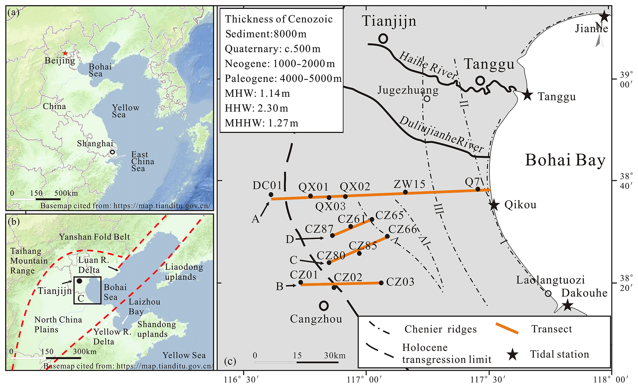
Figure 1 The study area: (a) location of Bohai Bay and Yellow Sea; (b) location of the study area and major river deltas; red dashed lines indicate the topographic boundaries of coastal lowland; (c) locations of boreholes, transects A, B, C, D, chenier ridges (Su et al., 2011; Wang et al., 2011) and Holocene transgression limit (Xue, 1993). The base maps of Fig. 1a and b are cited from “map world” (https://www.tianditu.gov.cn/, last access: June 2020, National Platform for Common GeoSpatial Information Services, China).

In our study area, observational data were firstly obtained from chenier ridges (Wang, 1964). Subsequently, a series of studies on marine transgression and lithostratigraphy provided the framework for understanding the late Quaternary evolution of Bohai Bay (e.g. Zhao et al., 1979; Fig. S1 in the Supplement), and over 130 Holocene sea-level data, generated in the study area over time since the early 1960s, have recently been compiled by Li et al. (2015; Fig. S2; for details see Supplement). However, because no correction for compaction was carried out, uncertainties were poorly constrained and no screening took place by which unsuitable material (e.g. transported shell) is rejected; the data set requires further scrutiny and is not used in our study. Instead, we established new sea-level data based on salt-marsh peat or peaty clay collected from drilling cores and compared with GIA model predictions. The difference between model and observational datum should allow inferring the non-GIA, and hence fluvial, impact on the sea-level history. We show here that shelf effect and local processes influenced the regional sea-level history at different times.

2 The study area

The study area lies in a mid-latitude, temperate climate zone (Fig. 1a) on the north-western coast of the East China Sea's wide shelf. Geologically, Bohai Bay is a depression filled by several kilometre-thick Cenozoic sediment sequences with the top 500 m ascribed to the Quaternary (Wang and Li, 1983). The long-term tectonic subsidence has been estimated to be about 1.3–2.0 mm a⁻¹ at Tianjin City (Wang et al., 2003). The Bay is a semi-enclosed marine environment, connected to the Pacific through a gap between Liaodong Peninsula and Shangdong Peninsula and the Yellow Sea (Fig. 1b). Our study area is the central coast of the Bay which lies between two deltaic plains, the Yellow River delta in the south and the Luan River delta in the north (Fig. 1b). Several small rivers (e.g. Haihe and Duliujianhe; Fig. 1c) cut through the coastal plain and enter the Bay. The coastal lowland is characterised not only by its low-lying nature (less than 10 m above sea level) but also by a series of chenier ridges situated south of the Haihe River and buried oyster reefs situated north of the Haihe River (Fig. 1c; Li et al., 2007; Su et al., 2011; Wang et al., 2011; Qin et al., 2017). Local reference tidal levels such as mean high waters (MHWs) and highest high waters (HHWs) are 1.25 and 2.30 m respectively based on the four tidal stations on the coast of Bohai Bay (Fig. 1c). During the Last Glacial Maximum the shoreline moved to the shelf break of the Yellow Sea, more than 1000 km to the east and southeast of our study area (e.g. He, 2006). During the Holocene the sea inundated the coastal area, with the shoreline moving about 80 km inland (e.g. Wang et al., 2015).

3 Methods

3.1 Sampling and elevation measurements

To obtain sedimentary sequences for this study, we consulted previous studies (e.g. Cang et al., 1979; Geng, 1981; Wang et al., 1981; Wang, 1982; Yang and Chen, 1985; Zhang et al., 1989; Zhao et al., 1978; Xue, 1993) to learn where in the bay marine deposits are dominant and where the landward limit of the last marine transgression should occur. We then collected 15 cores along W–E transects from the modern shoreline to 80 km inland (Fig. 1c), using a rotary drilling corer. Transect A, comprising six cores, stretches from the modern shoreline 80 km inland and crosses the inferred Holocene transgression limit (Xue, 1993). Transects B, C and D, comprising nine cores, cross the transgression limit a little further south (Fig. 1c). The surface elevations of the drilled cores were levelled to the National Yellow Sea 85 datum (or mean sea level, m.s.l.) using a GPS-RTK system with a precision of 3 cm. The GPS-RTK raw data were corrected and processed to the National Yellow Sea 85 datum system by the CORS system network available from the Hebei Institute of Surveying and Mapping with National measurement qualification.

3.2 Sediment and peat analyses

In the laboratory, the sediment cores were opened, photographed and recorded for sedimentary characteristics including grain size, colour, physical sedimentary structures and content of organic material. To study the degree of marine influence in the muddy sediment sequences, subsamples were collected at 20 cm intervals. These were analysed with respect to diatoms and foraminifera with a subsequent focus on the foraminifera due to the poor preservation of diatoms. The foraminifera of the >63 µm fraction of 20 g dry sample were counted (e.g. Wang et al., 1985) following studies on modern foraminifera (e.g. Li, 1985; Li et al., 2009). Sediment description followed Shennan et al. (2015): where in the sediment sequences foraminifera first appear and/or significantly increase (from zero or less than 10 to more than 50), this is noted as transgressive contact, while the sediment horizon where foraminifera disappear and/or decrease significantly is noted as regressive contact. These changes are often associated with lithological changes, such as from salt-marsh peaty sediment to estuarine sandy sediment or tidal muddy sediment across a transgressive contact or vice versa. In addition, peat material was analysed in terms of its foraminifera content so that salt-marsh peat can be differentiated from freshwater peat.

3.3 Analysis of compaction

Because the Holocene marine deposits are mainly unconsolidated clayey silt with around 0.74 % organic matter (Wang et al. 2015) post-depositional auto-compaction (Brain, 2015) may have led to a lowering of the sea-level index point (SLIP). According to Feng et al. (1999), the water content and compaction of marine sediments show a positive correlation with the down-core reduction in water content of the Holocene marine sediment being about 10 %. Based on these observations, we assumed the maximum lowering is about 10 % of the total thickness of the compressible sediment beneath each SLIP. Consequently, the total lowering for an affected SLIP is 10 % of the total thickness of the compressible sequence beneath the dated layer divided by the post-depositional lapse time proportional to the past 9000 years (e.g. Xiong et al., 2018), i.e. since the marine transgression in the study area.

3.4 Radiocarbon analyses

Sixty-nine bulk organic sediment samples from salt-marsh peat were collected from drilling cores, and the peat or plant subsamples obtained from these bulk sediments were chosen for AMS radiocarbon analysis at Beta Analytic Inc. because these can give more reliable ages than shells for the SLIPs. The resulting raw radiocarbon ages were converted to conventional ages after isotopic fractionation was corrected based on δ¹³C results. The conventional radiocarbon ages were calibrated to calendar years using the data set Intcal13 included in the software Calib Rev 7.0.2 for organic samples, peat and plant samples (Reimer et al., 2013). Because Shang et al. (2018) reported age overestimation of 467 years for the bulk organic fraction of salt-marsh peaty clay compared to the corresponding peat fraction, all the AMS ¹⁴C ages between 4000 and 9000 BP obtained from salt-marsh samples were corrected by $Y=\mathrm{0.99}X-\mathrm{466.5}$ (Y is the corrected age, X is the age obtained from the organic fractions; Shang et al., 2018) except for one <600 years in age from borehole Q7 (Table 1).

Table 1 Analytical data used to establish SLIPs.

^a Sediment compaction: 10 % of compressible thickness divided by lapse time of deposition in the past 9000 years. ^b Corrected for marine influence on salt-marsh organic sample fraction ages of peaty clay. NA: not available.

3.5 Sea-level index points

To develop SLIPs, salt-marsh peaty clay layers were used. To convert the dated peat layers into a SLIP, the modern analogue approach was used by measuring the elevation of the modern open tidal flat (Fig. 2) and sampling its surface for their foraminiferal content. Following the studies of the modern foraminifera assemblage (Li et al., 2009) Ammonia beccarii typically occurs in the upper part of an intertidal zone and Elphidium simplex in the lower intertidal zone. The zonation of the modern foraminifera assemblage was then used to identify the indicative meaning of the salt-marsh peat layers: the palaeo mean sea level is the midpoint between high water of spring tides (HHW: +2.3 m) and mean high waters (MHW: +1.25 m), which is 1.78 m with ±0.53 m uncertainty (Wang et al., 2012, 2013; Li et al., 2015). For each dated salt-marsh peat layer the indicative meaning and range, the total amount of possible lowering in elevation due to sediment compaction, and the reconstructed elevation of palaeo mean sea level are listed in Table 1.

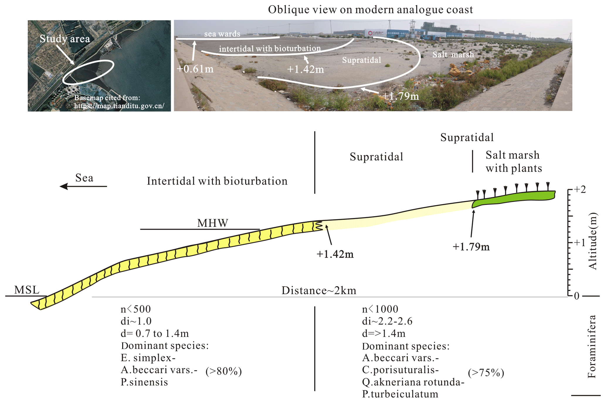
Figure 2 Schematic cross section of the modern tidal flat of the study area showing two characteristic foraminiferal zones. The base map of study area is derived from “map world” (https://www.tianditu.gov.cn/, last access: June 2020, National Platform for Common GeoSpatial Information Services, China).

3.6 GIA modelling

The time evolution of the sea level was obtained using the open-source program SELEN (Spada and Stocchi, 2007) to solve the “sea-level equation” (SLE) in the standard form proposed in the seminal work of Farrell and Clark (1976). In its most recent development, SELEN (version 4) solves a generalised SLE that accounts for the horizontal migration of the shoreline in response to sea-level rise, for the transition from grounded to floating ice and for Earth's rotational feedback on sea level (Spada and Melini, 2019). The programme combines the two basic elements of GIA modelling (Earth's rheological profile and ice melting history since the Last Glacial Maximum) assuming a Maxwell viscoelastic incompressible rheology. The GIA models adopted are ICE-5G(VM2) (Peltier, 2004), ICE-6G(VM5a) (Peltier et al., 2012) (both available on the home page of W. R. Peltier), and the one developed by Kurt Lambeck and colleagues (National Australian University, denoted as ANU hereafter; Nakada and Lambeck, 1987, Lambeck et al., 2003) provided to us by Anthony Purcell (personal communication, 2016). Table S1 summarises the values used for each model. The palaeo-topography has been solved iteratively, using the present-day global relief given by model ETOPO1 (Amante and Eakins, 2009). All the fields have been expanded to harmonic degree 512, on an equal-area icosahedron-based grid (Tegmark, 1996) with a uniform resolution of ∼ 20 km. The rotational effect on sea-level change has been taken into account by adopting the “revised rotational theory” (Mitrovica and Wahr, 2011).

4 Results

4.1 Lithostratigraphy and facies

Lithostratigraphically, the cores show a succession of terrigenous (including freshwater swamp, river channel, flood plain), salt-marsh and marine sediments (Table S2) with a clear W–E trend from terrestrial to marine dominance of deposits (Figs. 3–6). Transect A, around 80 km long, shows this trend: close to the modern shoreline pre-Holocene terrigenous sediments are overlain by basal peat including salt-marsh peat or peaty clay. Further inland these are replaced by freshwater peat overlain by salt-marsh and intertidal sediments and, above that, by terrigenous sediments. The cores DC01, CZ01 and CZ02 are composed of fluvial sediments only, roughly confirming the Holocene maximum transgression inferred by Xue (1993). Multiple shifts between salt-marsh, marine and fluvial deposits are noticeable in cores QX02, QX03 and CZ61, which originate from the central part of the study area.

Figure 3 The lithostratigraphy of transect A, with details of dated sedimentary horizons.

Figure 4 Foraminiferal counts from five cores of transect A. Counts >500 are shown as 500.

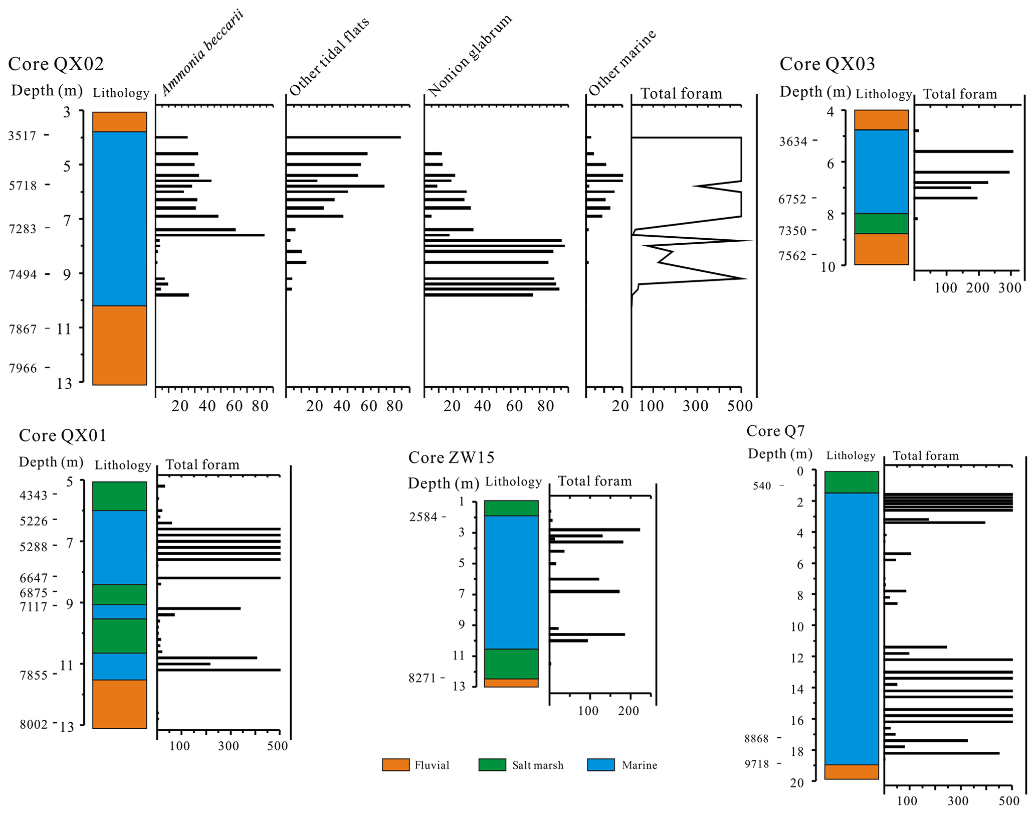
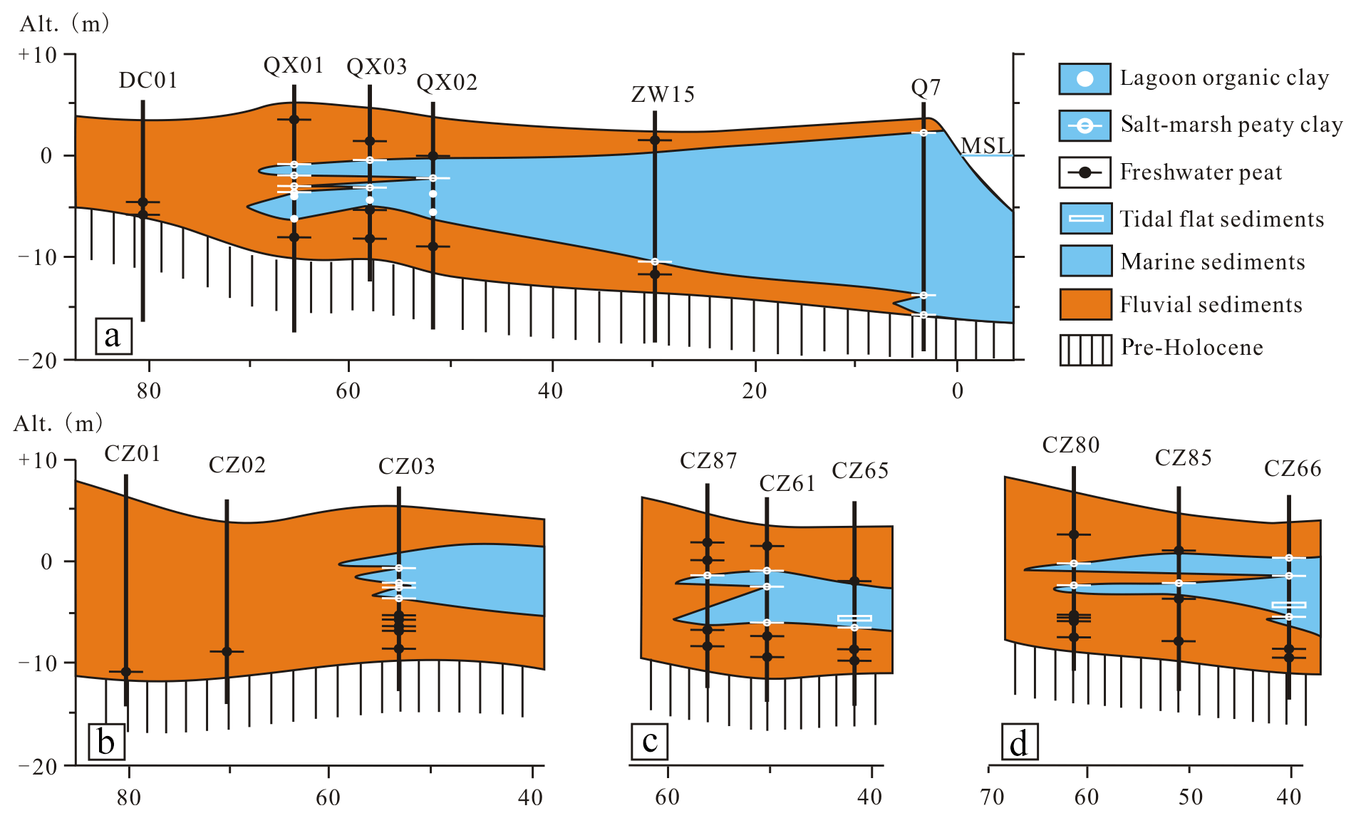
Figure 5 The lithostratigraphy of transects B, C and D, with details of dated sedimentary horizons.

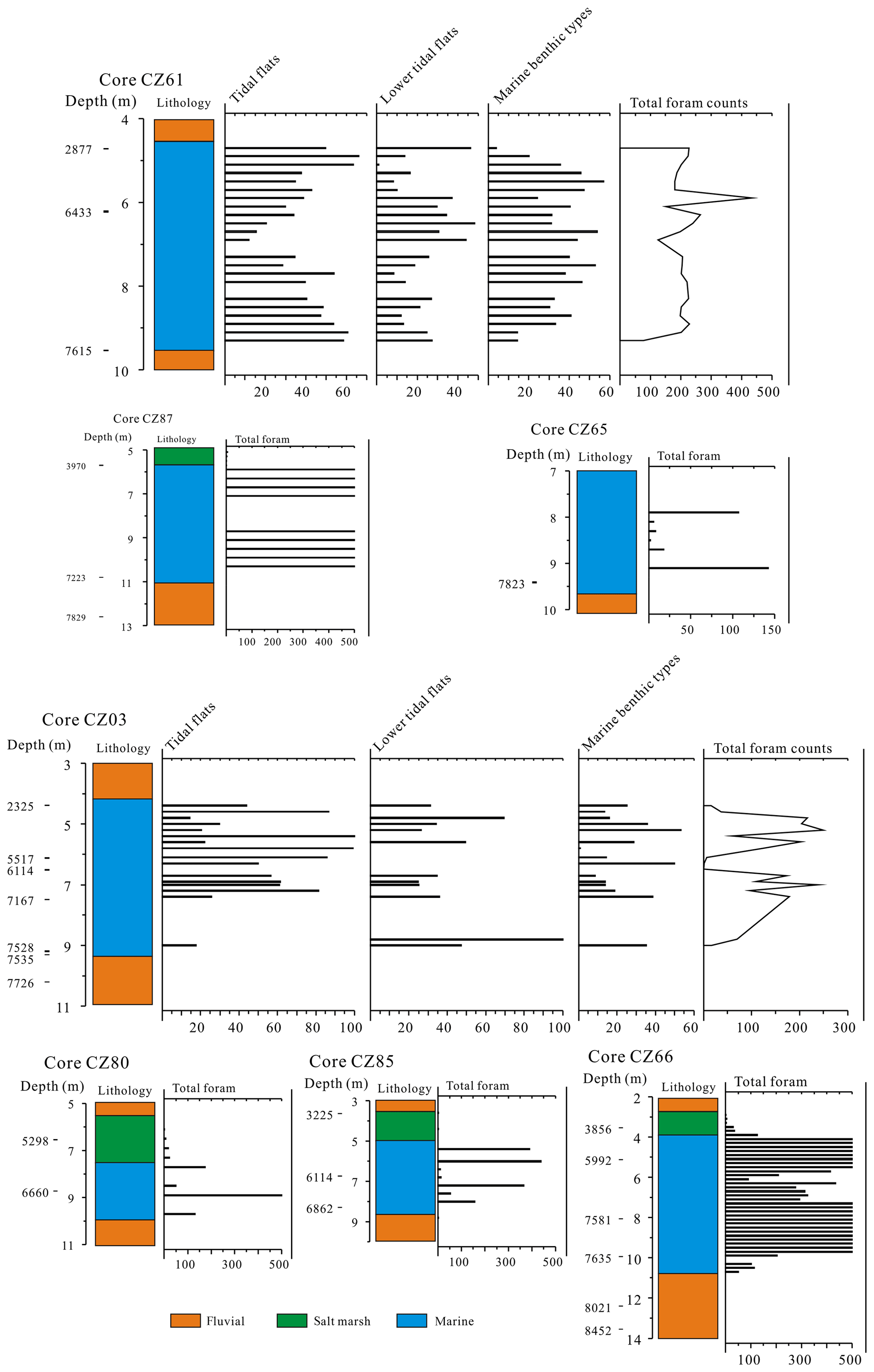
Figure 6 Foraminiferal counts from five cores of transects B, C and D. Counts >500 foraminifera are shown as 500.

Marsh deposits are either a blackish and thin freshwater peat mostly interbedded in yellowish fluvial sediments or a yellowish-brown salt-marsh peat bearing intertidal foraminifera (Table 1). Their lower boundaries are usually sharp, and their upper boundaries are mostly diffused or the salt-marsh peat changes gradually into dark grey intertidal sediments. Salt-marsh peat is intercalated in marine sediment sequences (i.e. QX01, QX02, CZ61, CZ85, CZ66 and CZ03; Figs. 3–6), particularly at sites that are close to the Holocene maximum transgression limit.

4.2 Foraminifera data

Foraminifera were identified in all cores except CZ01, CZ02 and DC01, which originate from the landward site of the maximum transgression limit. As Figs. 4 and 6 show, foraminifera start to appear at 11.2 m depth, which is dated to about 7.85 ka cal BP in QX01. The abundance of fossil foraminifera changes from about 404 to 772 individuals per samples at depths from 11.2 to 10.8 m, from 68 to 338 specimens from 9.4 to 8.8 m and from 103 to 3456 counts from 8.2 to 7.6 m. The assemblages reach maximum abundance at 6.6 m depth, which is dated to between 5.29 and 5.23 ka cal BP, with over 30 000 individuals per sample, before disappearing at 5.6 m. Dominant species change from Nonion glabrum in 11.2–7.4 m to Ammonia beccarii vars. in 7.4–6.4 m. This change represents a change from a salt marsh to a lagoon. In QX02, the pattern of foraminifera distributions is very similar. Low numbers of foraminifera, mostly Nonion glabrum, start to appear at about 10.1 m (−6.53 m of sea level), as dated to between 7.87 and 7.49 ka cal BP. The abundance reaches its highest at 6.7 m (−3.13 m of sea level), and the assemblages were dominated by Ammonia beccarii vars. Foraminifera disappear sometime between 5.72 and 3.52 ka cal BP. In all seaward drilling core – CZ03, CZ80, CZ85, CZ66, CZ87, CZ61, CZ65, ZW15 and Q7 – the pattern of foraminifer distributions are very similar to those at QX01 and QX02 (Fig. 4). The foraminifera start to appear in low numbers in the layer just above the basal peaty clay. This first appearance is at c. 17–8 m depth dated to 9–7 ka cal BP. Above this depth the count increases from ∼100 to ∼3000 foraminifera per sample at c. 8–7 m depth. The maximum count with >30 000 individuals per sample is reached at −6–5 m dated to around 5 ka cal BP. Foraminifera disappear in these cores sometime between 5.7 and 3.5 ka cal BP. The foraminifera assemblage is composed of few species only; hence it is not rich and is first dominated by Nonion glabrum at 17–7 m depth and then dominated by Ammonia beccarii vars. at 7–6 m depth. Other species found are Quinqueloculina akneriana rotunda and Protelphidium tuberculatum (Figs. 4 and 6).

4.3 Modern analogue and indicative meaning and range

The data obtained from the modern analogue show that the tidal flat can be divided into two sub-environments: intertidal with bioturbation (worm hole developed in tidal surface) and supratidal with salt-marsh vegetation (Fig. 2). Within the supratidal and salt-marsh zones, the foraminiferal assemblages are dominated by Ammonia beccarii, covering an elevation range from +1.42 to +2.00 m, including the +1.79 m boundary of salt marsh with plants. At sites below these elevations, i.e. intertidal with bioturbation (Fig. 2), the foraminiferal assemblages are dominated by Elphidium simplex, Ammonia beccarii and Pseudogyroidina sinensis. This foraminiferal zone covers an elevation ranging from 1.42 m to modern mean sea level.

Besides occasional A. beccarii there are few living foraminifera in the salt marsh above the MHW. The abundance is either biased towards Ammonia beccarii or it is relatively small. The latter is most probably due to the area being situated above the MHW and, hence, subject to evaporation during low tide, with the consequence of a relatively high and highly variable salt content of the pore water in the intertidal zone. The modern analogue samples confirm the bias towards salt-tolerant species (Fig. 2, Table 1). The spatial distribution of the ages confirms the E–W trend of the Holocene transgression where the oldest age is close to the modern shoreline and the youngest age is close to the maximum transgression limit.

4.4 Sea-level index points

In total 25 sea-level index points were established from the dated basal salt-marsh peat using the information obtained from the modern analogue. In Core Q7, at the most seaward location in the study area, the basal SLIP is dated to ∼9700 cal BP (Table 1), marking the onset of marine inundation of the study area. The overlying marine sequence is capped by a thick layer of shelly gravels at 1.30 m depth, and the associated SLIP is dated to 540 cal BP. This marks the upper end of the marine sequence as foraminifera start to disappear alongside a change from intertidal to supratidal environmental conditions. The cores ZW15, QX02, QX03 and QX01 show the same sequence as Q7 and provide six SLIPs. Nineteen SLIPs were collected from other cores (Table 1).

5 Discussion

5.1 Quality of SLIP data

Owing to the elevated and variable salinity of the coastal water, samples from both cores and modern tidal flat are characterised by low microfauna diversity and a low number of foraminifera species. This precludes the use of transfer function statistics and compels analysis based on direct comparison with the modern environment. We have solved this analytical problem by establishing SLIPs exclusively from basal salt-marsh peat in transgressive contact and by correcting the data for compaction. This analytical rigour allowed generating more accurate and more precise SLIP data than those reported by Li et al. (2015) because these earlier SLIP data are characterised by relatively poor chronological and elevation control (for details see Supplement). Notwithstanding SLIP improvement in terms of accuracy and precision, fluctuation of the data exists that can exceed 1 m (e.g. at 3.9 and at 5.2 ka; Fig. 7). Although hard to prove due to lack of data, we believe that these fluctuations are caused by groundwater extraction which lowers the surface in places.

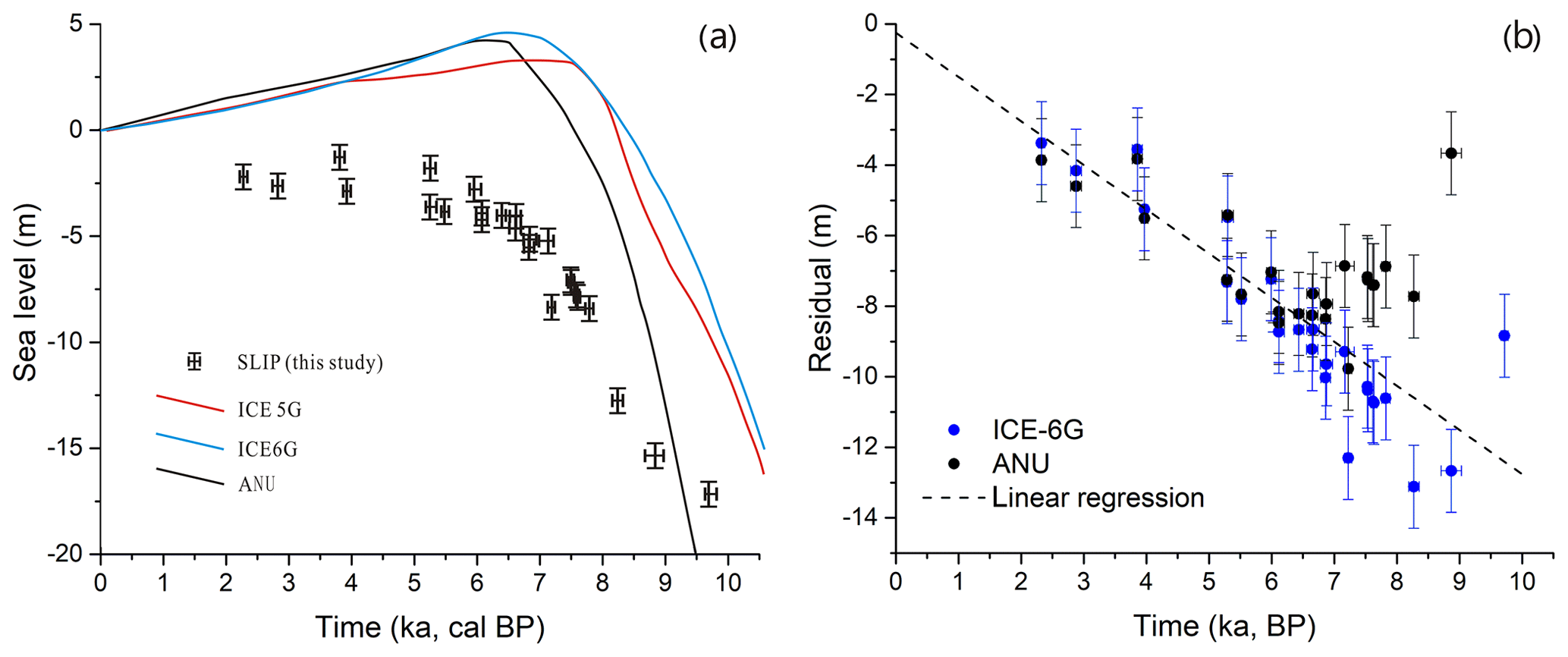
Figure 7 Observed and predicted sea level in Bohai Bay and resulting residuals: (a) SLIPs generated in this study and sea-level predictions. ICE-5G, ICE-6G and ANU are GIA models described in Sect. 3.6. Lithospheric thickness (km): 65 (ANU), 90 (5G and 6G); upper mantle viscosity (Pa s): 0.5×10²¹ (ANU, 5G, 6G); lower mantle viscosity (Pa s): 10×10²¹ (ANU), 2.7×10²¹ (5G), 3.2×10²¹ (6G); see also Table S1; age error bars are too small to be clearly visible. (b) Sea-level residuals plotted against time. Residuals are the difference between SLIPs and interpolated model data points. Error bars are derived from SLIP uncertainties. The trend line (dashed line) is computed as a least-squares regression on the mean residuals obtained with ANU and ICE-6G. The regression line approximates zero elevation remarkably closely, which gives confidence that the calculated 1.25 mm a⁻¹ for the non-GIA component is correct.

5.2 The observed Holocene sea-level rise

The SLIPs established indicate two phases of sea-level rise during the Holocene. The first phase occurred in the early Holocene until ∼6.5 ka when the sea level rose from −17 to −4 m. The second phase occurred from ∼6.5 to 2 ka when the sea level rose from −4 to −2 m. The oldest Holocene shoreline in Bohai Bay is, situated at −17.2 m at ∼9.7 ka cal BP, similar to Tian et al. (2017), who indicate $\sim -\mathrm{20}$ m at 9.4 ka cal BP based on seismic units and drilling cores. Between around 8.8 ka and 7.5 ka cal BP the sea level rose rapidly from −15.4 to −7.0 m at a rate of c. 6.4 mm a⁻¹. Then, from 7.5 ka to 5.2 ka cal BP the relative sea level rose to −3.6 m at an average rate of 1.9 mm a⁻¹ and to −1.2 m until 3.8 ka cal BP, before falling to −2.1 m at 2.3 ka cal BP with an average rising rate of c. 0.4 mm a⁻¹ from 5.2 to 2.3 ka cal BP. The final phase from 2 ka to today is constrained by only one SLIP from core Q7 dated to 540 cal BP at ∼0.5 m (Table 1). Lithostratigraphic data (Shang et al., 2016) suggest that the surface of the intertidal sediment body remained very close to 0 m from the landward limit of the marine transgression to about 2 km inland from the present shoreline. Further inland, in borehole ZW15 the surface elevation of the same intertidal sediment body is ∼3.0 m lower than in core Q7 (Figs. 3 and 4) suggesting a rise of sea level in Bohai Bay in the last 1000 years.

5.3 Observed and predicted Holocene sea level

We compare our observational data with GIA models employed in this study and with Bradley et al. (2016; henceforth denoted as BRAD; see also Table S1), who examined several ice-melting scenarios together with a range of Earth model parameters and validated model outputs using published SLIP data from the East China Sea coast including Bohai Bay.

Figure 7a displays observational data and sea-level predictions generated in this study. It shows that none of GIA models approximates the observations. The difference ranges between around 14 m at 9 ka and 3 m at 2.5 ka. Bohai Bay's oldest Holocene shoreline (∼9.7 ka cal BP) is at −17.2 m (observed), at c. −35 m (ANU) or at c. −10 m (ICE-X). The BRAD model predicts this shoreline to be at $\sim -\mathrm{20}$ m at 10 ka. Our observed shoreline elevation is similar to Sunda Shelf (c. −15 m; Hanebuth et al., 2011) but different to the islands of Tahiti (c. −28 m; Bard et al., 2010) and Barbados (c. −25 m; Peltier and Fairbanks, 2006). There are two ways to interpret this: (i) the age of the lowermost SLIP in core Q7 is overestimated due to old carbon contamination of the dating material, or (ii) the relatively shallow shoreline position in our study area is a deviation from eustasy due to the levering of the broad continental shelf in response to ocean load (e.g. Milne and Mitrovica, 2008). The similarity to the Sunda Shelf and the absence of contamination elsewhere in the sediment cores does indeed suggest that the broad-shelf effect (East China Sea shelf; Fig. 1) causes the shallow shoreline position. More SLIP data are needed to provide unequivocal evidence for it.

While SLIP data suggest a rising rate of ∼0.4 cm a⁻¹ during the early Holocene, the GIA models indicate ∼0.5 cm a⁻¹ (ICE-X) and ∼0.9 cm a⁻¹ (ANU). The ICE-X models approximate the observed early Holocene rising rate, but the timing of this rise is offset by about 2000 years. In the ANU model the early Holocene sea level rises almost twice as fast as the observed one with an offset of ∼500 years. Thus, the observed early Holocene sea level rises slower than the modelled sea level. For the mid to late Holocene SLIP data suggest ∼0.04 cm a⁻¹ rising rate, while the GIA models indicate a falling sea level. Predictions obtained from ICE-5G and ICE-6G are generally relatively similar but deviate from each other in the timing of the mid-Holocene sea-level highstand. The GIA models, including BRAD, show the highstand (4.6 m–3.4 m; 0.5 m) at 7–6 ka, while the SLIP data remain below modern sea level until 2 ka. The misfit between observed and predicted sea-level rise is much smaller in the coastal zone south of Bohai Bay than in our study area (Fig. S3). This should reflect the geological structure of the area: our study area belongs to the North China Plain Subsidence Basin (Wang and Li, 1983), while the south of Bohai Bay lies on the edge of Shandong Upland (Fig. 1b). Thus, the most likely explanation for the Bohai Bay misfit is subsidence of the coastal plain. Subsidence is a non-GIA component and should become evident through the residuals (i.e. the difference between observation and prediction per unit of time; Fig. 7b). Indeed, we identify the linearity of residuals for the period 7–0 ka, suggesting that subsidence dominates the local sea-level signal after the rise of the eustatic sea level has slowed down. A subsidence rate of 1.25 mm a⁻¹ is estimated from the residuals, similar to Wang et al. (2003), who deduced a rate of ∼1.5 mm a⁻¹ from the 400–500 m thick Quaternary sequence in the bay. It is possible that fluvial sediment supply enhanced the subsidence rate in the Holocene. The Yellow River's annual discharge into Bohai Bay is estimated to be 0.2 Gt until 740 CE rising to 1.2 Gt until around 1800 when widespread farming on the Loess Plateau started increasing the river's sediment load (Best, 2019). Thus, the sea-level rise in Bohai Bay is in the early Holocene dominated by the eustatic sea-level rise and GIA effects associated with the broad shelf from the Bohai Sea to the East China Sea, while in the mid to late Holocene it is dominated by a combination of tectonic subsidence and fluvial sediment load.

6 Conclusions

Using advanced methods for field survey and identification of accurate and precise sea-level markers, we have established a new Holocene sea-level history for central Bohai Bay. Our new data are not only different to previously published data in that they do not show the expected mid-Holocene sea-level highstand, but they are also different to global GIA models. We see a possible broad-shelf effect elevating the shoreline by several metres in comparison to the tropical islands of Tahiti and Barbados, and we see local processes controlling shoreline migration and coast evolution as soon as ice melting ceased. This indicates that more emphasis should be placed on regional coast and sea-level change modelling under a future of global sea-level rise as local government needs more specific and effective advice to deal with coastal flooding.