the Creative Commons Attribution 4.0 License.
the Creative Commons Attribution 4.0 License.
 | 20 Nov 2020
Erosional response of granular material in landscape models
Claudio Faccenna
Francesca Funiciello
Fabio Corbi
Sean D. Willett
Tectonics and erosion–sedimentation are the main processes responsible for shaping the Earth's surface. The link between these processes has a strong influence on the evolution of landscapes. One of the tools we have for investigating coupled process models is analog modeling. Here we contribute to the utility of this tool by presenting laboratory-scaled analog models of erosion. We explore the erosional response of different materials to imposed boundary conditions, trying to find the composite material that best mimics the behavior of the natural prototype. The models recreate conditions in which tectonic uplift is no longer active, but there is an imposed fixed slope. On this slope the erosion is triggered by precipitation and gravity, with the formation of channels in valleys and diffusion on hillslope that are functions of the analog material. Using digital elevation models (DEMs) and a laser scan correlation technique, we show model evolution and measure sediment discharge rates. We propose three main components of our analog material (silica powder, glass microbeads and PVC powder; PVC: polyvinyl chloride), and we investigate how different proportions of these components affect the model evolution and the development of landscapes. We find that silica powder is mainly responsible for creating a realistic landscape in the laboratory. Furthermore, we find that varying the concentration of silica powder between 40 wt % and 50 wt % (with glass microbeads and PVC powder in the range 35 wt %–40 wt % and 15 wt %–20 wt %, respectively) results in metrics and morphologies that are comparable with those from natural prototypes.
- Article
(9761 KB) - Full-text XML
- BibTeX
- EndNote


Whenever tectonics create topography, erosion and surface processes act in response to the imposed gradient, tending to reduce topography and, with time, remove all relief. During the last decades a strong theoretical background has been built based on field and analytical observations (e.g., Howard, 1994; Kirby and Whipple, 2001, 2012; Tucker and Whipple, 2002; Whipple et al., 1999; Whipple and Tucker, 1999, 2002), but since natural observations provide only a snapshot of processes acting at different timescales (e.g., Castillo et al., 2014; Cyr et al., 2014; Pederson and Tressler, 2012; Sembroni et al., 2016; Vanacker et al., 2015) a quantitative framing of the existing feedbacks between surface processes and tectonics in modifying topography remains a difficult task. Analytical, numerical and analog models are often used by tectonic geomorphologists to improve the understanding of the feedbacks between tectonics and surface processes. Numerical models have the advantage of a straightforward quantitative and parametric approach and the possibility to be conducted with precise boundary conditions. Previous numerical and analytical studies have focused on the following: the mathematical implementation in solving the stream-power law (Braun and Willett, 2013); the interaction between surface processes and the velocity discontinuities bounding a double-verging orogenic wedge (Braun and Yamato, 2010); the coupling between climate, erosion and tectonics (e.g., Batt and Braun, 1999; Beaumont et al., 1992, 2001, 2004; Jamieson et al., 2004; Ueda et al., 2015; Whipple and Meade, 2004); the interaction between surface processes and multilayer folding systems (Collignon et al., 2014); the role of orographically enhanced precipitation in a double-verging 2-D model (Willett, 1999; Willett et al., 1993); the control exerted by tectonic strain (Castelltort et al., 2012; Duvall and Tucker, 2015; Goren et al., 2015); and interaction with tectonics in three dimensions (Ueda et al., 2015). Nevertheless, the computational capacities necessary to realistically simulate geologic features coupled with erosion using complex rheologies and/or three-dimensional settings still place strong limitations on numerical runs. Furthermore, spatial features such as spacing of rivers are often mesh-dependent, making them a function of the modeler input of the mesh resolution.
Analog models can in principle overcome these limitations, allowing a useful direct control on the evolution of the studied physical process (e.g., Reber et al., 2020). These are free to evolve following the physics acting on them without needing external control apart from boundary conditions. The coupling between tectonics and surface processes has been investigated using sandbox-like analog apparatuses including removal of material by hand or with a vacuum cleaner (e.g., Hoth et al., 2006; Konstantinovskaya and Malavieille, 2011; Malavieille et al., 1993; Mulugeta and Koyi, 1987) and the application of a defined precipitation rate for a spontaneously developing landscape (e.g., Bonnet, 2009; Lague et al., 2003; Schumm and Parker, 1973; Tejedor et al., 2017). The former models can be considered “dry” models in which no water is added to the system. In this case, brittle wedges are typically built, and after a certain amount of shortening the material is removed from the wedge and sifted in the lower basins. The latter models can be considered “wet” because water is added to the system and is responsible for erosion, transport and sedimentation. Wet models mainly focus on surface uplifting and lowering (e.g., Bonnet and Crave, 2003; Hasbargen and Paola, 2000; Ouchi, 2011; Schumm and Rea, 1995; Singh et al., 2015) or creating topography by horizontal advection (e.g., Graveleau et al., 2015; Graveleau and Dominguez, 2008; Guerit et al., 2016; Viaplana-Muzas et al., 2019). Different granular materials have been used, like dry quartz sand (e.g., Persson et al., 2004), silica powder (e.g., Bonnet, 2009), mica flakes (e.g., Storti et al., 2000), glass microbeads (e.g., Konstantinovskaya and Malavieille, 2011), natural loess (e.g., Lague et al., 2003), walnut shells (e.g., Cruz et al., 2008) and ad hoc composite materials (e.g., Graveleau et al., 2011, 2015). These materials show different behavior in response to the external forcing, and their characterization is a key ingredient for scaling analog models. The link between the properties of the materials and their tuning on the morphological response is not well defined yet. Even if some recent efforts have been made with pure materials and mixes (e.g., Bonnet and Crave, 2006; Graveleau et al., 2011), an excursus on the role played by the concentration of every component in a composite material is still lacking.
Here we focus on analog materials, exploring how different concentrations of granular materials influence the erosional, physical and mechanical response of several composite materials with the overarching goal of finding a material that best mimics the erosional behavior of the natural prototype. We also focus on mechanical properties of the same materials, which will be involved in future projects.
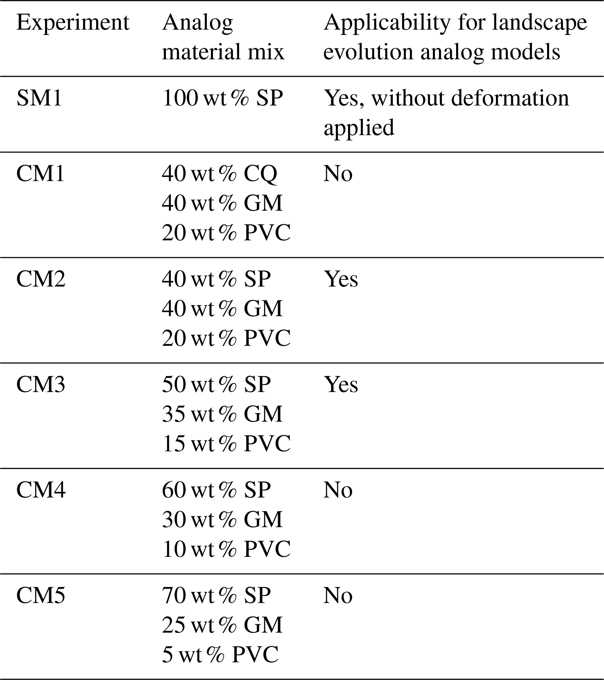
In this study we analyzed four different brittle granular materials to be used as rock analogs for the upper crust: silica powder (SP), glass microbeads (GM), crushed quartz (CQ) and polyvinyl chloride (PVC) powder. These pure materials are used in five different mixes in different proportions, while one single material (SP) is tested on its own (Table 1). The selection has fallen on granular materials for the following reasons.
- a.
They have the proper physical properties to simulate downscaled crustal rock behavior under laboratory conditions in a natural gravity field (e.g., Davis et al., 1983; Lallemand et al., 1994; Mulugeta and Koyi, 1987; Schreurs et al., 2001, 2006, 2016; Storti et al., 2000; Storti and McClay, 1995). As a matter of fact, they obey the Mohr–Coulomb failure criterion, showing strain hardening prior to failure at peak strength and strain softening until a stable value is reached (stable friction) (Lohrmann et al., 2003; Schreurs et al., 2006).
- b.
They reproduce reasonable geomorphic features due to the development of erosion and sedimentation processes like incision, mass wasting and diffusive erosion, transport, and sedimentation, although important differences in behavior and characteristics have emerged (Graveleau et al., 2011, 2015; Graveleau and Dominguez, 2008; Viaplana-Muzas et al., 2019).
In the following, we describe (a) geotechnical characterization of the materials (including geometrical, physical and chemical properties, frictional properties, and permeability), (b) erosional characterization and (c) scaling to the natural prototype. We also define which conditions a proper analog material should satisfy to be used in landscape evolution models.
Table 1Material used in experiments. The label CM indicates a composite material, while the label SM indicates a pure single material.
2.1 Mechanical properties
Here we describe the mechanical properties of four granular materials mixed in different proportions. The aims of this analysis are to study how mechanical properties affect erosion style and to define properties that will be used in future works for which the materials will be involved in experiments where active tectonics and erosion act simultaneously. In five experiments the analog material are mixtures of the previous materials at various percentages (CM1-5, Table 1). In Graveleau et al. (2011), the authors describe how these different pure materials (except CQ, which was not considered in their work) show advantages and disadvantages in responding to erosion and sedimentation in terms of morphological features developed and brittle behavior. For example, GM and PVC produce high scarps with almost no channelization when erosion is applied but realistically reproduce the brittle rheology of the upper crust (Graveleau et al., 2011). SP morphologies scale well with natural landscapes, but the higher strength of the powder induces unreliable structures under deformation. To overcome the above limitations of materials used as single “ingredient”, the authors suggested that a mixture of these three granular materials can be the most appropriate choice. Following Graveleau et al. (2011), here we focus on these mixes rather than pure materials. The latter are still analyzed, highlighting their role in the mix.
We measured geometrical, physical and frictional properties such as grain size and shape, density, porosity and permeability, internal friction angle, and cohesion. We measured frictional properties of experimental granular material (internal friction coefficient μ and cohesion C) with a Casagrande shear box. We performed tests for peak and stable friction at variable normal stresses. Density has been measured with a helium pycnometer. The grain size has been estimated via a series of sieves of decreasing opening dimensions (from 250 to 45 µm). The material passing the 45 µm sieve has been analyzed using sedimentation in a distilled-water tank, with a hydraulic pump for recirculation of water and a thermal control for estimation of water density. We also used a laser diffractometer for checking the reliability of the previous measurements. A qualitative analysis has been carried out using a scanning electron micrograph (SEM) for the shape of grains and composition.
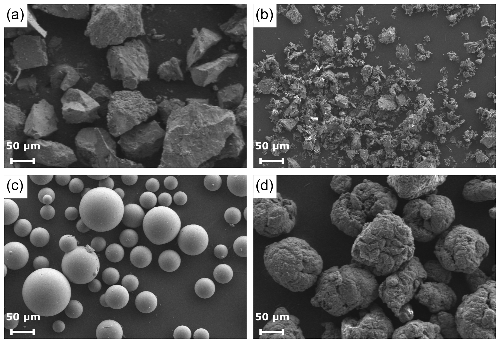
Figure 1SEM (scanning electron micrograph) pictures of the materials tested in this work. (a) Crushed quartz, (b) silica powder, (c) glass microbeads, (d) PVC powder.
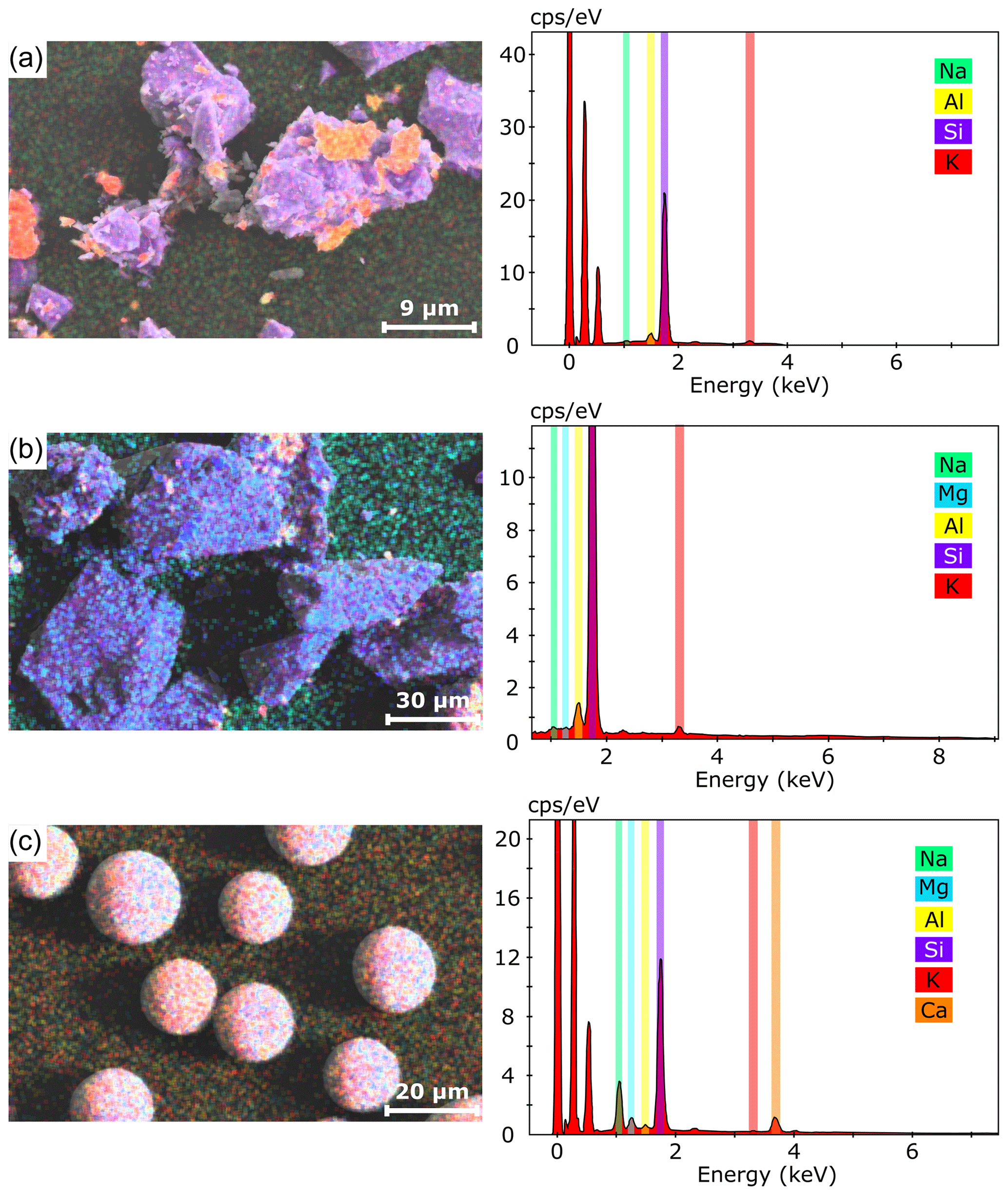
Figure 2SEM qualitative analysis of the material composition. On the left is the backscattered electron (BSE) imaging, while on the right is the energy-dispersive detector (EDS) spectrum. A qualitative composition is presented for (a) silica powder, (b) crushed quartz and (c) glass microbeads. PVC powder has not been analyzed due to its complex composition.
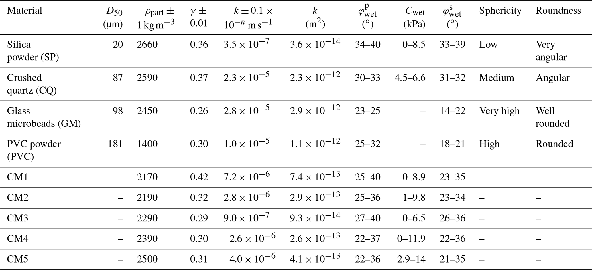
Table 2Geometrical and physical properties of pure granular materials and mixes. Here we show values for grain size (D50), particle density (ρpart), porosity (γ), permeability (k), cohesion (C), and internal friction angle for peak () and stable () friction. Sphericity and roughness have been estimated after the acquisition of SEM imaging. The subscripts dry and wet indicate whether the tests were made with dry materials or water-saturated materials.
2.1.1 Geometrical and physical–chemical properties
The material physical properties like grain size, density, porosity and permeability are listed in Table 2. The SP is a very fine powder (D50 = 20 µm), with clasts of different shape and size (Fig. 1): the smallest ones are elongated and may lay on bigger clast with a very high roughness. These characteristics require a careful use of this powder due to danger for the respiratory system. The density is the highest among the studied components (2660 ± 1 kg m−3). We obtain compositions of ∼ 95 % SiO2, ∼ 3 % Al2O3, ∼ 1 % K2O, and < 1 % Na2O, MgO and CaO (Fig. 2). The CQ has bigger dimensions with respect to SP (D50 = 87 µm), with medium sphericity of the clasts and high roughness. The composition is very similar to silica powder (with ∼ 0.5 % FeO) and so is the density, which is slightly lower (2590 ± 1 kg m−3). GM (D50 = 98 µm) has a very high sphericity and a very low roughness, with a density (2450 ± 1 kg m−3) lower than the CQ. The GM qualitative composition is ∼ 69 % SiO2, ∼ 15 % Na2O, ∼ 10 % CaO, ∼ 4 % MgO, ∼ 1 % Al2O3, and < 1 % K2O and fluorine. Finally, the PVC (D50 = 181 µm) has a similar shape with respect to glass microbeads but less uniform. The density is the lowest among the components (1400 ± 1 kg m−3), and this has a strong effect on the erosive properties of the material, as we will show afterwards. We did not perform SEM measurements with the PVC due to the complexity of its chemical composition ((C2H3Cl)n). The grain size, density and shape of grains in the mixes are a function of the percentage of every single material that forms it (Table 2).
2.1.2 Frictional properties
A good crustal analog material must fail following the Mohr–Coulomb failure criterion (e.g., Davis et al., 1983; Davy and Cobbold, 1991; Krantz, 1991):
where τ is the shear stress corresponding to the normal stress σ on the failure plane, and μ is coefficient of internal friction defined as μ=tan(φ), with φ the angle of internal friction. For geomorphic experiments in which water is added to the system, parameters like μ and C strongly control the evolution of the experiment because they change with the amount of water. The brittle granular materials typically used in laboratory models have low elasticity and undergo plastic deformation when their yield strength is reached, sliding along discrete fault-analog planes (e.g., Panien et al., 2006; Ritter et al., 2018; Rossi and Storti, 2003; Schreurs et al., 2016). Deforming granular materials satisfy the Mohr–Coulomb criterion (Eq. 1), which highlights the relationship between shear stress τ and normal stress σ on the failure plane. The criterion typically shows a linear trend for σ of the order of kilopascals (kPa) and megapascals (MPa) but a convex-outward envelope for normal stresses of the order of hundreds of pascals (Pa) or lower (Schellart, 2000). In this work the normal stress applied is in the 25–200 kPa range. Estimation of normal stress at the base of our models is about 1 kPa. The experimental tests are then only an underestimate of the real mechanical behavior within the models. Nevertheless, the tests provide useful insight into the frictional properties of the analog materials. For every test (four tests per material) we defined peak friction (the first peak in the shear curve in Fig. 3 reflects hardening–weakening during strain localization and then fault initiation) and stable friction (the plateau after peak friction represents friction during sliding; e.g., Montanari et al., 2017). A shear box has been used. It consists of a steel box (Rossi and Storti, 2003) split across its middle into two small blocks with an area of 6 cm × 6 cm each. The bottom block is fixed, while the top block moves at a constant velocity of 0.165 mm min−1. Two dynamometers record horizontal and vertical displacement. The tests were made in water-saturated conditions. From every measurement we defined the material internal friction coefficient (μ, slope) and cohesion (C, intercept) for peak and stable friction. Results for every material and mix are listed in Table 2. Among the pure materials SP shows the highest values for φ and C (34–40∘ and 0–8.5 kPa, respectively). For GM the internal friction angle is about 23–25∘ and the cohesion is close to 0 or negative, so is not considered in this analysis. PVC shows the same conditions for C, with an internal friction angle between 25 and 32∘. The frictional properties for the CQ are similar to SP, with φ between 30 and 33∘ and C between 4.5 and 6.6 kPa. The mixes show a strong variability for φ and C, with average values of about 31∘ and 6 kPa, respectively. The values of φ and C do not highlight the increasing of SP concentration from CM2 to CM5.

Figure 3Ideal output from a shear test. The peak friction corresponds to the high point of the curve, while stable friction is defined by the subsequent plateau.
2.1.3 Porosity and permeability
Porosity is defined as the ratio between the volume of voids or pore spaces (VV) and the total volume (VT):
The porosity has been computed by measuring the volumetric change in a weighted amount of material with respect to an ideal condition in which no pores are in the samples. We used a vibrating plate, looking for the best compaction of material, and measured the variation in volume. We used this technique to draw close to the experimental conditions. This procedure has been repeated several times for each composite material. Unfortunately, porosity is dependent on the handling technique; it is thus impossible to precisely control the porosity of the materials during preparation. The values of porosity for single materials and mixes are shown in Table 2. We also measured porosity by weighing the same volume of material in water-saturated conditions and after drying it in an air oven. The results are directly comparable between the two different measurement techniques. GM shows the lowest porosity (0.26) among the pure materials, while SP and CQ show the highest (0.36 and 0.37, respectively). As far as the mixes are concerned, only CM1 shows values higher than 0.40, while porosity is around 0.30 from CM2 to CM5.
Permeability represents the ability of a material to transmit fluids. This property has been tested using an odometer and measuring the velocity of water flowing through the sample. This parameter is essential in controlling the evolution of our models, as will be explained later in the text. SP has the lowest permeability (3.6 × 10⁻¹⁴ m2), while GM has the highest permeability (2.9 × 10⁻¹² m2). CM1 shows the highest permeability among the various mixes (7.4 × 10⁻¹³ m2). From CM2 to CM5 (from 40 wt % and 70 wt % SP) the permeability slightly decreases. However, CM3 and CM5 do not strictly follow this trend: the former has the lowest permeability observed in mixes (9.3 × 10⁻¹⁴ m2), while the latter shows a value comparable with CM2 and CM4 but slightly higher (4.1 × 10⁻¹³ m2). The permeability values for mixes are then in the order of 10−13 m2.
2.2 Erosional characterization
2.2.1 Erosion laws and erosive properties
In a stream channel, the relationship between channel slope S and contributing area A is often expressed through Flint's law (Flint, 1974) and takes the form
where ks and θ are the steepness and concavity index, respectively. The most common erosion law, consistent with slope-area scaling, for channelized processes is a power-law function of the contributing area A and surface gradient S, defined as the “stream-power” law (e.g., Howard, 1994; Tucker and Whipple, 2002; Whipple and Tucker, 1999):
where z is the elevation of the stream channel (i.e., dz∕dt elevation trough time), K is the erosional constant (bound up to the erosional efficiency) that contains information about lithology, climate and channel geometry (Howard et al., 1994; Whipple and Tucker, 1999), and m and n are two positive dimensionless exponents, with the ratio m∕n (i.e., the concavity index θ) that typically falls between 0.4 and 0.7 (Tucker and Whipple, 2002). This model is better known as a “detachment-limited” stream-power model because in tectonically active regions or in condition of steep topography, the channel erosive power is high and limited by its capacity to detach particles from the bedrock (Tucker and Whipple, 2002; Whipple and Tucker, 2002). It is possible to rewrite Eq. (4) in terms of distance x along the stream using Hack's law (Hack, 1957):
where ka is a scaling coefficient and H is the reciprocal of the Hack's exponent. Combining Eqs. (4) and (5) we obtain
where κ = . In our experiments, K, κ, m, n and H should be constant (for the same experiment) due to the homogeneous lithology and constant precipitation rate.
A proper analog material for landscape evolution models should erode via localized area-dependent processes (i.e., advection in valleys), diffusion (i.e., on hillslopes) and mass wasting. Primarily, it must develop channelization in response to accumulated flow. This requires precipitation to collect in surface drainage networks, with branching channels in order to be consistent with Hack's law and slope-area scaling. For the erosional behavior of the composite material, the ratio between precipitation rate and infiltration capacity appears to be the main factor controlling the geomorphological response. If the precipitation rate is higher than the infiltration capacity, the model can develop surface runoff (Graveleau, 2008). Otherwise, the water flows through and inside the model, inducing fast erosion through discrete and rapid events. Fine sand or powders have typically been used for geomorphic experiments (e.g., Babault et al., 2005; Hasbargen and Paola, 2000) so that runoff could develop (i.e., low infiltration capacity due to the grain size). Nevertheless, different materials exhibit different emergent morphological characteristics when precipitation is imposed. Among the pure materials presented above, only SP (or a mix with SP) successfully reproduces linear incision (e.g., Bonnet and Crave, 2006; Graveleau et al., 2011; Schumm and Parker, 1973; Tejedor et al., 2017), while GM, PVC (Graveleau et al., 2011) and CQ erode mostly by diffusion or mass wasting.
2.3 Experimental setup for erosional characterization
For studying the composite material response to applied boundary conditions (precipitation rate and slope), we developed a new experimental setup of depositing the material into a box on an inclined plane under rainfall (precipitation). Both the initial slope for the apparatus and the precipitation rate are kept constant. No kinematic conditions of sidewalls are applied: no active tectonics are thus reproduced in our model.
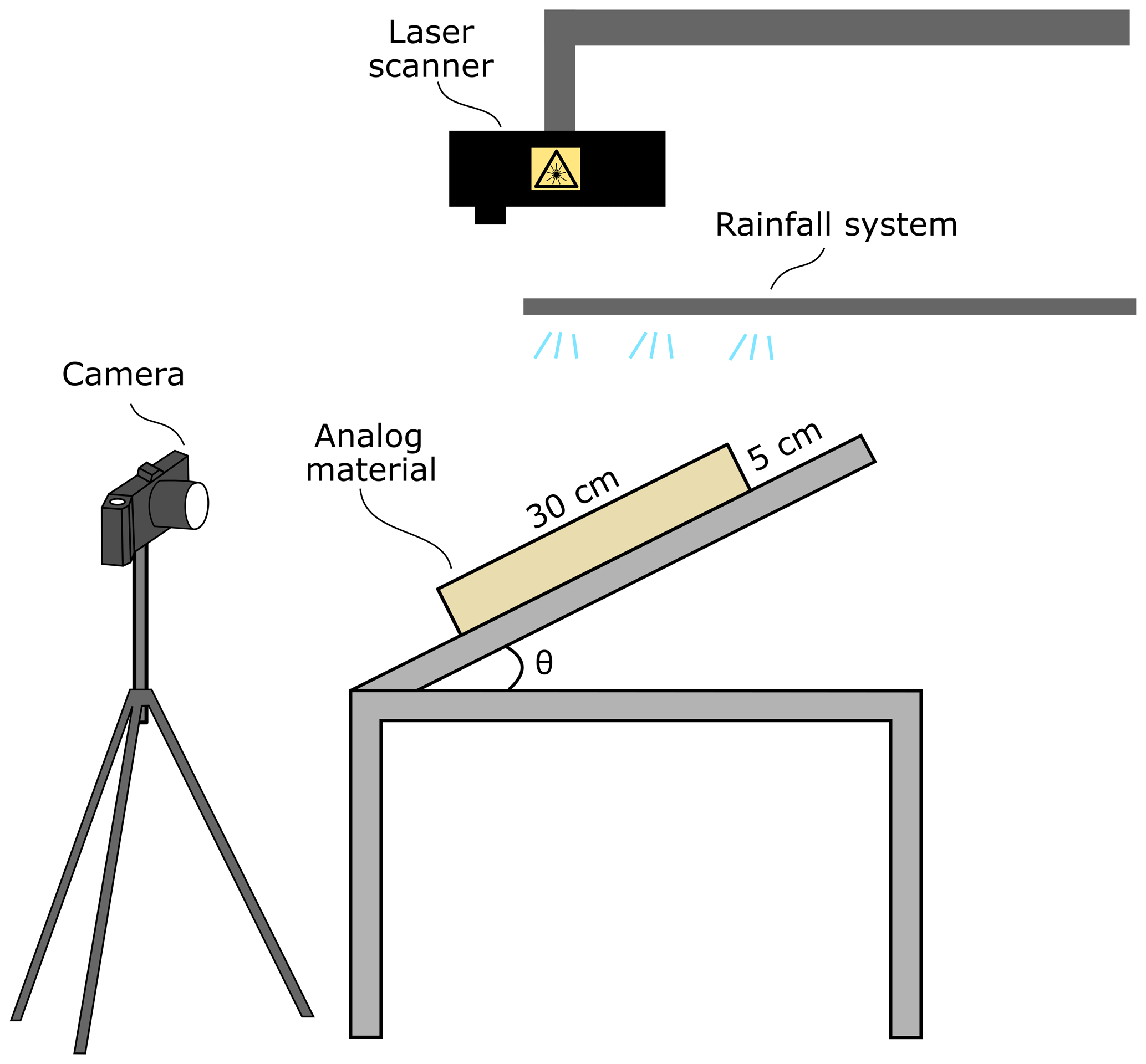
Figure 4Schematic representation of the experimental setup used for models with only erosion: block of experimental material (35 cm × 30 cm × 5 cm), rainfall system (commercial sprinklers) and reclining table. A single camera and a high-definition laser scan provide records for the experiments.
The experimental setup is made of three different devices (Fig. 4): the box, the rainfall system and the monitoring systems. The material box controls the imposed initial slope, while the rainfall system triggers surface erosion. The evolution of the model is recorded with digital images and a laser scanner. The only forcing applied to the models is due to gravity acceleration, which allows for the erosion triggered by slope and rainfall.
2.3.1 Box
The box is a Plexiglass tank 0.35 m × 0.3 m × 0.05 m filled with the water-saturated experimental material (about 25 wt %). After pouring the material into the box and leveling, it is left flat for at least 12 h to avoid prior deformations. The slope of the box is then fixed at 15∘, in analogy to what has been done in Graveleau et al. (2011).
2.3.2 Rainfall system
Three nozzles fixed to an aluminum frame produce a high-density fog in which the droplet size is small enough (≤ 100 µm) to avoid rain-splash erosion (e.g., Bonnet and Crave, 2006; Graveleau et al., 2012; Lague et al., 2003; Viaplana-Muzas et al., 2015). The precipitation rate is controlled by both water pressure and the number of sprinklers. In our models the precipitation rate is fixed to 25–30 mm h−1. The configuration allows for a homogeneous droplet distribution with a spatial variation of about 20 %. The precipitation rate induces surface runoff, channel incision and gravity-driven processes that are responsible for the erosion of the model.
2.3.3 Monitoring system
Each experiment is recorded using one camera and a laser scanner. The camera records the model evolution in oblique view. The laser horizontal and vertical resolutions are 0.05 and 0.07 mm, respectively. The scans are converted into digital elevation models (DEMs) using MATLAB. DEMs are analyzed with TopoToolbox (Schwanghart and Scherler, 2014) for geomorphological quantifications. Erosion and sediment discharge are computed with ad hoc MATLAB algorithms (see “Data availability” to access the codes). Stopping the rainfall and letting the surface dry are required to avoid distortions during the laser scan. For the first hour pictures and scans are taken every 15 min, then every 30 and 60 min, depending on the model evolution rate.
2.4 Scaling analysis
An analog model should be scaled by its geometry as well as its kinematic, dynamic and rheological properties (e.g., Hubbert, 1937; Ramberg, 1981). The length scaling factor (h∗ = hmodel∕hnature) commonly used in sandbox experiments for deformation in the upper crust with granular material ranges between 10−5 and 10−6 (e.g., Cruz et al., 2008; Davy and Cobbold, 1991; Konstantinovskaya and Malavieille, 2011; Persson et al., 2004; Storti et al., 2000). Hence, 1 cm in the model may be in the range of 1–10 km in nature. The gravitational acceleration model-to-nature ratio is set to 1 (g∗ = gmodel∕gnature) working in the natural gravitational field. The density of the dry quartz sand or corundum sand employed in the literature defines the model-to-nature ratio for density (ρ∗ = ρmodel∕ρnature) to be around 0.5–0.6. Since the dimensionless coefficient of internal friction is very similar between the analog material and the natural crustal rocks, the cohesion and body force scaling factor can be expressed as
Typical values of this scaling factor are of the order of 10−6 so that 1 Pa in the model would correspond to about 1 MPa in nature (e.g., Buiter, 2012; Graveleau et al., 2012).
The classical approach in analog modeling of convergent wedges is time-independent (i.e., the evolution of the model is independent from the convergence rate). Here, together with compressional tectonics we also model erosion with the perspective of implementing the tested materials in analog models in which tectonics and erosion are coupled. Therefore, following Willett (1999), we introduce a time scaling factor t∗, which is the ratio between the mass flux added to the system Fin and the mass flux removed Fout. Fin is defined as follows:
where vc and h are the convergence velocity and initial thickness of the layers considered, respectively. Fout is defined as
where K is a constant proportional to bedrock incision efficiency and precipitation rate (Eqs. 4 and 6), and L is the wedge width. Assuming m = 0.5 and n = 1 in Eq. (4) (e.g., Whipple and Tucker, 1999), the K parameter has the dimension of t−1. Therefore, the mass balance can be expressed as the ratio between these two fluxes:
Mb is a dimensionless number, so keeping it the same in the experiment as in nature (in the same gravity field) it is possible to derive the scaling factor for time by rewriting Eq. (10) as
and considering K∗ to have the dimension t−1 so that
where ∗ marks the model-to-nature dimensionless ratio for every quantity, as defined before. With this scaling factor, considering L∗ = h* = 10−5–10−6 and = 8 × 10⁻⁴, 1 min in the model corresponds to 3.8–38 kyr in nature.
Experimentalists are always in search of a perfect dynamic scaling for their models. Scaling all the aspects of geological processes is very difficult to achieve, if not impossible (Reber et al., 2020). For example, using granular materials leads to a length scaling inherently not perfect: grains of the order of 0.1–1 mm in the laboratory, assuming a length scaling factor of 10−5, would correspond to 10 to 100 m in nature, which is obviously overestimated. For landscape evolution models even more issues are linked to fluid flow or sediment transport (Paola et al., 2009). Nevertheless, these experiments provide an “unreasonable effectiveness” (Paola et al., 2009) that allows for their interpretation in terms of scaling by similarity (Reber et al., 2020). When the models and their natural prototype behave in a similar way, it is indeed possible to infer information about the prototype by studying the processes acting on the model (Reber et al., 2020) because of the scale independency of the processes.
We present six different models carried out with the same boundary conditions (i.e., imposed slope, precipitation rate and experimental time) and different mixed materials (Table 1). The same models have been conducted multiple times to ensure the reproducibility of the experimental results. The results presented in this paper are just a selection from amongst these repetitions. We tested mixes with different concentrations of CQ, SP, GM and PVC, accounting for the differences in erosional responses, starting from what is already known in the literature. These materials (except CQ) are also used in Graveleau et al. (2011) for the author-selected mix, named MatIV, composed of 40 % SP, 40 % GM, 18 % PVC and 2 % graphite powder. The same mix is represented here by CM2, wherein PVC is 20 wt % due to the absence of graphite. Therefore, this mix has been set as our reference model for further analysis. From this starting point, we increased the SP concentration (from 40 wt % to 70 wt %, from CM2 to CM5), lowering the GM and PVC concentration. Two experiments were carried out using only SP (SM1) and a mix with the same proportion of CM2 but with SP replaced by CQ (CM1).
The analysis illustrates erosional properties, showing the influence of different compositions on the morphology of the landscape, the river longitudinal profile, sediment discharge and erosion. All eroded material leaves the system; therefore, sedimentation is not modeled.
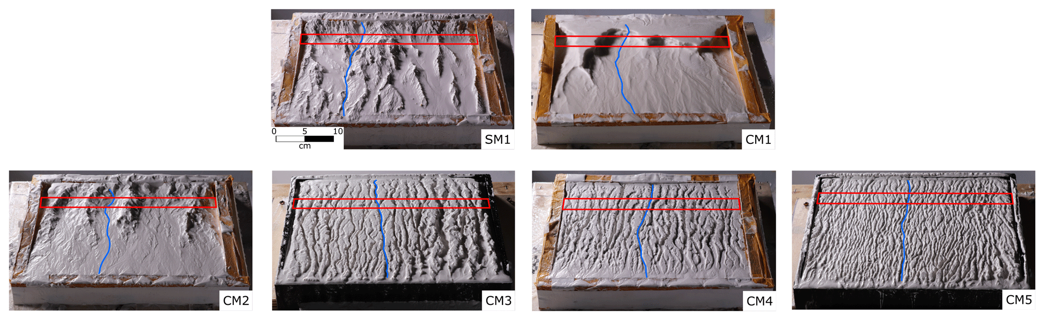
Figure 5Pictures of the models at 200 min from the beginning of the experiment. The red box is the trace of the swath profiles shown in Fig. 6. The blue line indicates the stream for every experiment analyzed in Fig. 7.
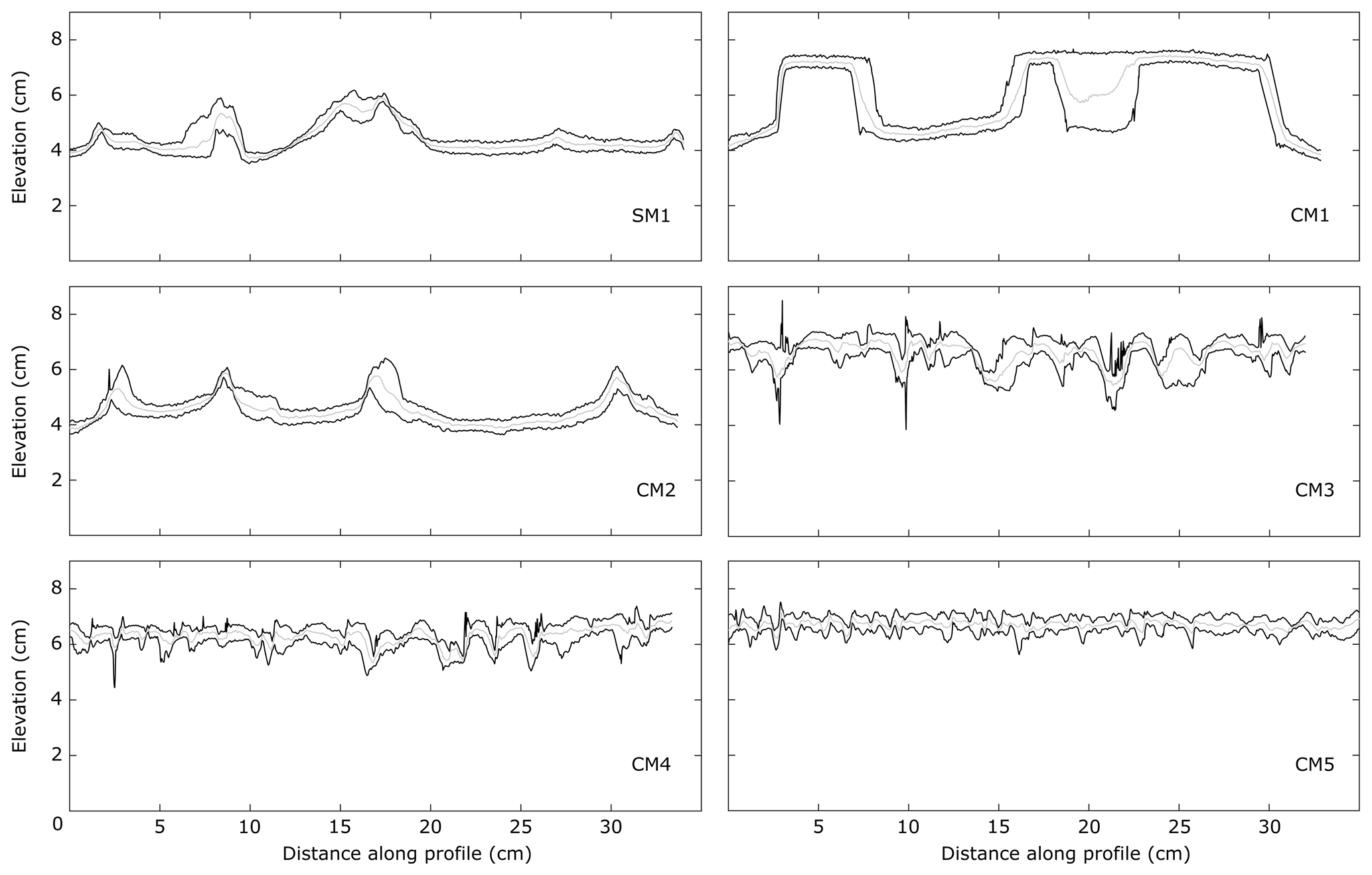
Figure 6Swath profiles transverse to the experiment slope. Profiles are plotted at the same experimental time at which the system keeps its morphologies almost constant through time (ca. 200 min). Location as shown in Fig. 5.
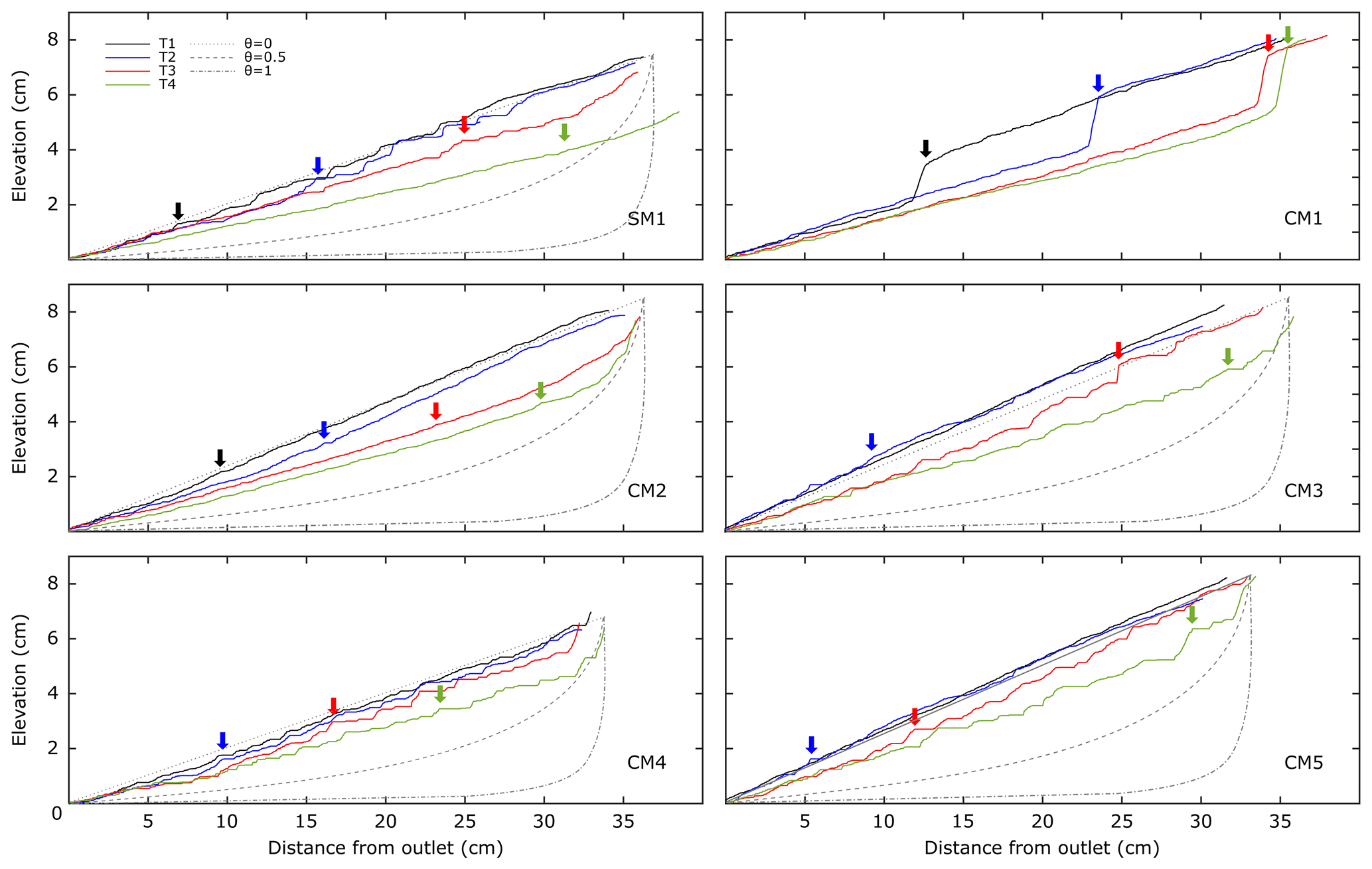
Figure 7Longitudinal profiles of the streams highlighted in Fig. 5. This analysis is performed by converting the laser scan into a DEM and applying the TopoToolbox tool for MATLAB (Schwanghart and Scherler, 2014). The laser horizontal and vertical resolutions are 0.05 and 0.07 mm, respectively. We show four profiles corresponding to four consecutive time steps (T1 = 20 min, T2 = 60 min, T3 = 150 min, T4 = 350 min). The vertical arrows point to the main knickpoints for the relative time step (color coding). In the figure theoretical river profiles for a concavity index of 0, 0.5 and 1 are also plotted. We did not plot the theoretical profile for CM1 because no proper channel develops (see text for details).
3.1 Morphology of erosion
In the reference experiment CM2 the rainfall system induces channel incision and triggers mass-wasting processes in a portion of the analog materials adjacent to stream channels. Both advection in channels and diffusion processes on hillslopes are present. A well-developed river network evolves 5 min after initiation. Single channels coalesce in basins with the increase in erosion, and they are separated by sharp ridges. Three main basins are located at the upper part of the model (Fig. 5). The planar surfaces developing close to the lowermost side of the experiment have a slope of about 9∘, which is 6∘ lower than the initial imposed slope. The bottom of the valleys and the peak are generally separated by 1–2 cm relief (Fig. 6). CM1 evolution differs substantially from the reference model CM2. No channel incision is observed (Fig. 5), while diffusion and mass wasting are the dominant processes. Two different planar surfaces are formed, separated by a vertical scarp convex-upward. An elongated elevated body stands close to the left boundary, related to the boundary effect itself. The planar surfaces have a slope of 12 and 10∘ for the lower and upper surface, respectively. The 12∘ slope is reached after 5 min from the beginning of the experiment when a proto-scarp is already formed. Subsequently, the scarp moves backward for about 60 min at a rate > 0.4 cm min−1, following which the scarp continues retreating but at a slower rate (< 0.1 cm min−1). The difference in elevation between the two planar surfaces is 2–3 cm. In the experiment SM1 channel incision is strong and affects the entire model. Almost no mass-wasting processes are observed. The landscape evolution for this model is similar to CM2. Four main basins are observed (Fig. 5), with a series of smaller basins linked to the major ones. Two of these basins stand on the leftmost part of the model and are separated by two main ridges (Fig. 6). The rightmost basins have a small ridge separating them. The ridges between different basins can attain a slope close to or even higher than 90∘. The planar surfaces that form at the end of the experiment have a slope between 9∘ and 10∘, which is 6∘ or 5∘ lower than the imposed initial slope. On the slopes bordering the basins several small channels form. Further increasing the SP concentration changes the erosional response of the model (Figs. 5 and 6). Channel incision becomes the main process acting on the model with the SP concentration from 40 wt % to 50 wt %. A further increase in the amount of SP produces more and narrower channels (Fig. 5). An anastomose system develops in CM5. In CM3, CM4 and CM5 the morphologies develop after around 10 min from the beginning of the experiment and are almost constant through the evolution of the models. No proper basin develops in these models, and there is no evidence of diffusive processes on hillslopes. As a matter of fact, swath profiles transverse to the rivers show strong variation in elevation with a small wavelength (Fig. 6). The valleys are sharp, very close to each other and not very incised.
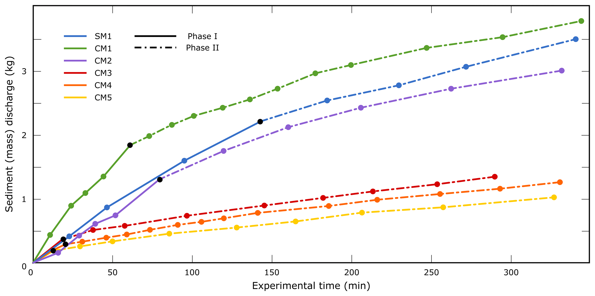
Figure 8Cumulative mass (sediment) discharge over time for the six experiments. The solid lines correspond to phase I, while dashed lines correspond to phase II. The black dot highlights the transition from phase I to phase II.
3.2 River longitudinal profiles
The river longitudinal profile represents the variation of stream elevation relative to the distance from the outlet. In Fig. 7 we show a river profile for each experiment at four different time steps. The river evolution in the reference model CM2 follows a well-known path, starting from the undisturbed initial slope and arriving at the final profile with a concave-upward shape. We can also observe how the propagation of the perturbation, from the initial condition, migrates from the outlet to the headwater as a knickpoint separating the transient from the equilibrium channel profile. In the upper parts of the model, the erosion removes up to 3–3.5 cm of material. In CM1 no proper river develops and the main knickpoint defines the entire topography, with two planar surfaces separated by a sharp scarp (Fig. 5). The experiments with CM3, CM4 and CM5 show a common behavior. Channels do not show a concave-upward shape, or maybe only in the uppermost part of the model, while generally straight rivers develop. Nevertheless, we can observe the propagation of the erosion wave from the bottom to the top. As in the other models, the incision is strong, but it does not produce very deep valleys (1.5–2 cm). Finally, in SM1 it is difficult to observe a proper concave-upward river profile. Some knickpoints in the earlier stage of river development are later obliterated (green profile in Fig. 7). The incision removes almost 3 cm in the northernmost portions of the model.
3.3 Sediment discharge and erosion
Sediment (mass) discharge can be characterized by the amount of material that leaves the model. Keeping the boundary conditions constant in all the experiments, evolution is only a function of the analog material composition. Sediment discharge plotted over time always shows two main phases (Fig. 8): phase I, fast removal of material from the model, and phase II, slower removal of material with a lower discharge rate that is kept constant until the end of the experiment. After an initial period in which the material quickly responds to the boundary condition with a high discharge rate that varies through time (the slope of the solid line in Fig. 8, phase I), the system reaches equilibrium with an almost constant discharge rate (the slope of the dashed line in Fig. 8, phase II). In the reference model CM2 and in SM1 this occurs when basins reach the dimension of 40–80 cm2. Different behaviors are shown by CM3, CM4 and CM5, for which phase I is extremely short (Fig. 8). In the reference model CM2, phase I lasts at least 80–90 min with a discharge rate around 15 g min−1, while for phase II it is 6 g min−1 (both values are comparable with SM1). In CM1 the discharge rate decreases from phase I to phase II, from ca. 31 g min−1 in the first 60 min to ca. 7 g min−1. The loss in discharge rate between phase I and phase II is around 76 % and corresponds, in time, to when the morphological evolution of the experiment significantly decreases, reaching an almost stationary condition. SM1 shows a similar trend, but a late and smoother transition from phase I to phase II happening after 140 min from the beginning of the experiment. The discharge rate is around 17 g min−1 during phase I and 6 g min−1 during phase II. A strong decrease in sediment discharge over time is observed between CM2 and CM3, while from CM3 to CM5 the difference is smaller. In CM3, CM4 and CM5 phase I is very short in time (< 20 min), with a discharge rate that decreases with an increasing SP concentration (from 19 to 13 g min−1). Phase II then lasts for the rest of the experiments, with a discharge rate of about 3 g min−1.
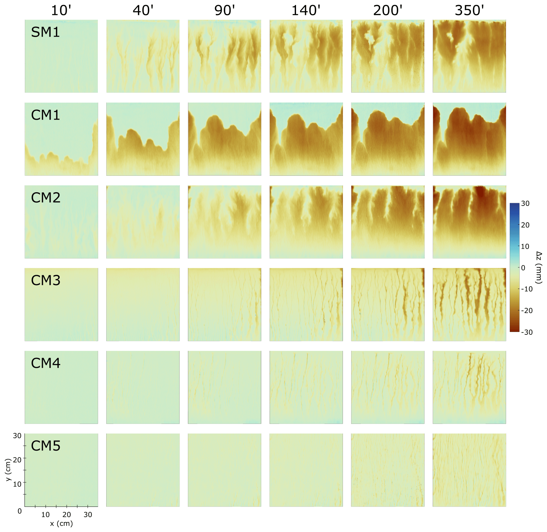
Figure 9Erosion evolution for the experiments, here represented by the cumulative difference in elevation (Δz) of the same point at consecutive times. Time is indicated in columns. Each row corresponds to a model; the mix adopted is indicated in the first panel of each row. The color coding is shown by the color bar on the right. Negative values correspond to erosion and positive ones to sedimentation (almost no sedimentation for these models).
In Fig. 9 we show the evolution of the erosion for the selected mix. In CM2 and SM1 river channels and basins are observed. In CM2 they are initially wider than in SM1. CM2 develops fewer basins, and they are less elongated. In CM2 the erosion appears to be more efficient, with a removal of material up to a depth of 3 cm in the uppermost portion of the model, close to the middle part of it. The erosion in CM1 follows the retreat of the scarps, and it is mainly focused from the scarp to 5–6 cm over the outlet (Fig. 9). It erodes at least 3 cm of the model, although no channels form. The erosion is likely homogeneous on the lower planar surface. The channel incision in CM3 is evident, and it reaches a depth of 2 to 2.5 cm. Here the erosion is focused in the channels, and they do not coalesce into basins. In CM4 and CM5 this affects the models even more. The erosion is extremely low, carving the models with incision lower than 2–2.5 cm (even lower in CM5).
The experimental setting presented in this paper allows for the investigation of the material and composite material response to the applied boundary conditions (15∘ slope and precipitation rate of 25–30 mm h−1). Despite simplifications (i.e., lack of tectonics, vegetation, storms, chemical weathering, seasoning, presence of infrastructures), these models highlight how the composition of the experimental material controls its erosional response. With respect to other works on the same topic (e.g., Bonnet and Crave, 2006; Graveleau et al., 2008, 2011), we focus on how varying the concentration of materials in a mix affect the models. Increasing the concentration of SP with respect to GM and PVC results in straighter channels and lower incision. Using CQ instead of SP results in an almost uniform morphology wherein no proper basins or channels form, and the erosion is mainly due to fast discrete events. Three main aspects arise from our results: (a) SP is a key ingredient to properly model erosion, (b) the physical properties of the experimental mix influence the sediment discharge rate and (c) the experimental results can be used to better understand how surface processes act in nature. These considerations lay the foundations for choosing the proper analog material for landscape evolution models. This indeed must satisfy conditions like morphology of the river channels, geomorphic indexes and erosional behavior that should fall in the range of natural observations. We find that the best analog material for landscape models settled in this work is represented by the composite materials used in models CM2 and CM3 (40 wt % SP, 40 wt % GM, 20 wt % PVC for CM2; 50 wt % SP, 35 wt % GM, 15 wt % PVC for CM3). Even if our compositions are comparable with the ones used in other laboratories (e.g., Graveleau et al., 2011), it is important to define how different combinations of the proposed materials may result in extremely different model evolution.
4.1 Comparison with previous works
The study by Graveleau et al. (2011) represents the recent foundation for modeling landscape evolution. Therefore, we start discussing differences and similarities of our results with respect to their study. In Graveleau et al. (2011) the authors tested four pure materials (silica powder, glass microbeads, PVC powder and graphite) and a single composite material (named MatIV). The composite material is composed of 40 % silica powder, 40 % glass microbeads, 18 % PVC powder and 2 % graphite. In our study we did not analyze graphite. We tested the effect of crushed quartz in composite materials instead. Concerning pure materials (silica powder, glass microbeads and PVC powder), our estimations and measurements for sphericity, grain size, density and permeability match the ones made by Graveleau et al. (2011) with unavoidable minor differences. We measured higher values of porosity for PVC, while permeability is of the same order of magnitude. Internal friction angles at peak and stable friction presented here are consistently lower for all our materials in comparison with Graveleau et al. (2011). The authors settled the tests at lower normal stresses than our measurements (< 5 and < 250 kPa). The Mohr–Coulomb failure criterion shows that when low normal stresses are applied to the sample, the failure envelope tends to steepen, inducing values of the internal friction angle higher than if measured at higher normal stresses (Schellart, 2000). This could explain the differences in results.
The composite granular material presented by Graveleau et al. (2011) (MatIV) has been proposed in this work as analog material used in CM2, except that graphite powder was replaced with a slightly higher amount of PVC powder (see the Results section for more details). Density, porosity and permeability are comparable with what has been measured by Graveleau et al. (2011) for MatIV. The values for peak friction and stable friction measured in this work are comparable to what has been measured by Graveleau et al. (2011).
The erosion of the models also shows similar evolution. The same rate for precipitation has been adopted in both works. We can observe strong similarity in the landscape reorganization between MatIV and CM2, looking at the frames in the evolution of the models at 15∘ slope (Figs. 9a–e and 10c in Graveleau et al., 2011, and Fig. 5 in this paper). The mass discharges over time (Fig. 9f in Graveleau et al., 2011, and Fig. 8 in this paper) for SilPwd (SM1 in this work) and MatIV coincide with our curves for SM1 and CM2 (at least for the first 90 min). During our phase II, the mass discharge observed in CM2 grows faster than MatIV (Fig. 9f in Graveleau et al., 2011). The mass discharge rate during phase II in CM2 is 6 g min−1, while in Graveleau et al. (2011) the discharge rate for MatIV is 2.8 g min−1.
The analytical approach regarding the temporal scaling proposed here (1 min = 3.8–38 kyr) can be compared with what has been proposed by Graveleau et al. (2011) and Strak et al. (2011). These authors proposed different approaches for time scaling with respect to this paper. However, they obtained the same order of magnitude of the model-to-nature scaling factors here proposed. In Graveleau et al. (2011), in a context tectonically quiescent, the authors compared erosion rate in models and in natural tectonically inactive areas starting from the geometric scaling. They estimated that 1 min in the models corresponds to 4.1–16.8 kyr in nature. In Strak et al. (2011) the authors compared the model denudation rate with the one computed for the Weber and Salt Lake City segments of the Wasatch fault, obtaining 1 min = 3.9–22.5 kyr. Both estimates fall in the range for temporal scaling proposed in this paper. The convergence of results gives reliability to the experimental method, which was carried out independently at two different laboratories and by different working groups.

Figure 10Box plot of the sediment discharge rate for phase I and phase II. The red lines indicate the median, and the bottom and top edges of the blue and brownish boxes indicate the 25th and 75th percentiles, respectively. The black markers outside the box cover the data point at < 25th and > 75th percentiles that are not considered outliers.
4.2 Silica powder for erosion models
SP is widely used in geomorphic experiments, showing a good qualitative response to erosion and sedimentation as well as developing geomorphic markers that morphologically approximate the natural prototype (e.g., Bonnet and Crave, 2006; Graveleau et al., 2011; Schumm and Parker, 1973; Tejedor et al., 2017). As already stated by Graveleau et al. (2011), pure granular materials such as SP, GM and PVC are not able to fully satisfy the requirements for our analog models. Pure GM and PVC show a deformational style characterized by a few localized thrusts and backthrusts, with a low surface slope around 10∘ that is coherent with the one of convergent margins (Graveleau et al., 2011). However, these materials fail to reproduce a realistic landscape morphology. SP shows the opposite behavior (Graveleau et al., 2011, and references therein). This material allows the models to develop streams, channels, basins and other geomorphic features, whereas deformation produces a high number of thrusts and backthrusts closely spaced and a taper slope higher than 14∘. A weighted mixture of these three components is then needed to fulfill the requirements for a scaled analog model in terms of deformation and erosional style. We managed to pin down silica as the main component in our composite materials, and we tested two different siliceous materials: CQ and SP. They are almost identical in their chemical composition (Fig. 2), but they strongly differ for grain size, sphericity and roughness (Fig. 1, Table 2). CM1 and CM2 have the same percentage of materials, but SP and CQ are switched. CM1 does not show channel incision, while CM2 is characterized by channel incision and mass-wasting processes (Fig. 5). Channel incision becomes the main process acting on the surface moving from CM2 to CM5 (from 40 wt % to 70 wt % of SP), but an increase in the number of channels (Fig. 5) produces less incised structures (Fig. 9). Despite 100 wt % SP, SM1 does not develop only straight channels, differing from CM3 and CM5. We can state that the morphological response to erosion depends on the geometrical and physical parameters rather than on the chemical ones (Figs. 5 and 8–10). Indeed, none of the materials chemically react with each other or with water. The ratio , where P is the precipitation rate and Ic the infiltration capacity, strongly controls the evolution of the experiments (Graveleau et al., 2011). When Sr < 1, Ic is greater than P and most of the water coming from the raining system is drained internally, inside the porous material. A flow at the interface between the model and the bottom of the box develops, triggering mass-wasting processes. This configuration makes it very hard to develop a well-defined surface runoff, and we could expect the same results as in CM1. On the other hand, when Sr > 1, the precipitation rate allows for the development of a river network at the model surface (as in CM2). Of course, it is possible to slightly change the precipitation rate according to the purpose of the experiment, but the main control on Sr is exerted by Ic. This parameter is a function of the permeability and, in turn, it is a function of the grain size, grain size distribution and (effective) porosity (Carman, 1938, 1956; Kozeny, 1927). These factors are responsible for the differences between CQ and SP and are then responsible for the results of CM1 and CM2 (same concentration of materials but with CQ and SP, respectively). In fact, the grain size of CQ is 1 order of magnitude higher than SP, and the latter has a higher grain size distribution (Fig. 1). Permeability spans over 2 orders of magnitude, from 2.3 × 10⁻¹² to 3.6 × 10⁻¹⁴ m2 for CQ and SP, respectively. The mix CM1 shows higher permeability than CM2. These considerations lead us to assess SP as the best siliceous material for landscape evolution models rather than CQ. But due to the very small grain size of SP, suction and capillary forces are very strong when water is involved. Consequently, other components become necessary to promote mass-wasting processes and for smoothing the mechanical behavior of SP to avoid unrealistic brittle structures (see Graveleau et al., 2011, and the beginning of this section). But going beyond what has already been done, we focused on testing how different combinations of SP, GM and PVC change the model results. Increasing the SP concentration should create configurations similar to SM1, but our results show that this is not the case. When SP is ≥ 50 wt % of the composite material, only straight channels form, and they are not so incised if compared with the ones from SM1 or CM2 (Figs. 5 and 9). CM3, CM4 and CM5 do not develop basins, and the erosion in the channels is limited (Fig. 9). Mass-wasting processes and gravitational processes are absent, and the rivers flow in narrow canyons. In CM5 the behavior is even more peculiar, and anastomose channels form with very low incision (Figs. 5 and 9). Thus, a mixture of SP, GM and PVC in which SP has the highest concentration develops forms that are very different from SM1, even if SP is 70 wt %. We propose here that this is mainly due to the grain size distribution. The voids between the grains of GM and PVC are most likely filled with the material with the lowest grain size, SP. If the concentration of SP is high enough (≥ 50 wt %) and water is added to the system, the strength of the material increases, and the erosional and mechanical response of the mix strongly changes. This is in agreement with measurements of frictional properties (Table 2).
4.3 Sediment discharge rate as a function of physical properties of analog materials
Phase I and phase II differ in terms of sediment discharge rate (SDR). Independently from the material, phase I displays higher SDR than phase II. In phase I the models equilibrate with the boundary conditions imposed. The amount of potential energy triggers a fast reorganization of the system. In the first time steps the materials quickly leave the models until the energy decreases and a new equilibrium is reached. Lowering the model slope toward an equilibrium shape slows down the erosional response of the model, entering phase II (Fig. 8). In this latter phase the system has reached a balance with the boundary condition, and SDR shows lower variability for a given model (Fig. 10). Despite these common points, features like the onset of the phases, their duration and the amount of discharged material differ among the models. During phase I all the models show high variability in SDR (Fig. 10). Nevertheless, CM1 still has the highest mean SDR (red line in Fig. 10) that later decreases from CM2 to CM5. CM1 erodes through fast and discrete processes (e.g., mass wasting), while all the other models also show (or only show) channel incision (Fig. 5). From CM2 to CM5 the SDR decreases. Due to the absence of chemical reaction between components and water, the differences in SDR are linked to the physical properties of the materials. In CM1 the subsurface water flow induces collapse of material in catastrophic events. In SM1 this does not happen. The very low permeability of the material inhibits significant subsurface flows. The erosion of the material is mainly linked to the ability of water to detach particles from the riverbed and carrying them outside the model. Initially, particles are detached when shear stresses exerted by water overcome the threshold for detachment of the grains in the analog materials (Howard, 1994). The strength of SP thus controls the rate of incision. There are similar considerations for CM2, but the higher permeability can trigger both channel incision and gravitational processes. Surprisingly, the CM3–CM5 response to precipitation rate is very different from SM1 or CM2. From CM3 to CM5 the SDR strongly decreases in both phases (Fig. 10), even if components like GM and PVC are added to the composite materials. The properties of these two pure materials would produce an erosional response similar to CM1 (Graveleau et al., 2011). However, when SP is in a proportion higher than 50 wt % the water capacity of detaching particles strongly decreases, so that even the incision is very shallow (Fig. 9), and so does the SDR. No mass-wasting processes act on these models, as suggested by the low permeability. We propose that the higher grain size distribution allows SP to fill the voids between the GM and PVC particles, lowering the permeability (Table 2) and increasing the material resistance with capillarity and electrostatic forces. In phase II the SDR variability is smaller, and the mean values are more representative of the whole SDR. The previous consideration of the role of grain size also applies in this phase, even if SDR is significantly lower. Up to now, we have talked about the balance between shear stress exerted by water and the strength of the riverbed as responsible for incision in the models. In the works from Lague et al. (2003) and Graveleau et al. (2011), the authors acknowledge the presence of an erosion threshold that must be overcome before significant erosion and transport occur. Graveleau et al. (2011) proposed that the tilted downstream zone observed in the models may be related to the presence of this erosion threshold. We also observe this tilted downstream zone, accounting likely for the same erosional threshold. In the experiments performed by Lague et al. (2003), all the experiments reach a final height of about 1 cm. This was independent of the initial condition. They related this limit elevation to an intrinsic threshold to erosion. They also approach the problem analytically, defining erosion laws in which a threshold term is present. Here, we recognized that the erosion threshold is mainly controlled by the mechanical strength of the materials used in the models, together with topographical parameters (e.g., gradient, river organization). From CM2 to CM5, the mechanical strength of the material appears to increase with the increasing concentration of SP in the mix, producing less incised landscapes, as highlighted by the morphologies (Fig. 5), the swath profiles (Fig. 6), the incision maps (Fig. 9) and the sediment discharge charts (Figs. 8 and 10).
4.4 Drainage network morphology
Our models are not meant to simulate any specific landscape but to explore how material properties influence landscape development. However, despite the unavoidable limitations and simplifications of the model, it is tempting to compare the experimental and natural data. To do so, one can make a comparison to Hack's law. Hack's law (Eq. 5) can be also written as
where L is the length of the channel in a basin, A is its drainage area, c is a scaling coefficient and h is the scaling exponent referred to as Hack's exponent. The scaling coefficient c and the scaling exponent h in Eq. (13) are related to ka and H in Eq. (5) by c = and h = 1∕H, respectively. Hack's law represents the relationship between channel length and drainage area and allows us to analyze the geometry of the drainage network. Dodds and Rothman (2000) show that in nature h is in the range 0.44–0.56, while c is between 1.3 and 6.6 (for individual basins compared at their outlets). In our models, SM1 and CM2 show the lowest values of h (< 0.8). The scaling coefficient c for SM1 and CM2 is in the range 1–4 and 0–4, respectively (between the 25th and 75th percentile) (Fig. 11). CM4 shows values for c and h close to 1 and in the range 0.8–1, respectively, while CM5 has a slightly larger distribution. CM1 and CM3 show the lowest values for the scaling coefficient c. Comparing the length-area scaling of our analog models with observations (Fig. 5) we notice that the models are characterized by a very low degree of branching of the drainage network. Moreover, our calculations of h are systematically higher than 0.5 (Fig. 11). Values of h greater than 0.5 are typically interpreted as indicating basin elongation with increasing size (Rigon et al., 1996). In fact, the drainage basins in our models are typically elongated, especially for CM3–CM5. SM1 and CM2 still have high values for h but lower with respect to the other models. For SM1 and CM2 the basins are morphologically better defined (Fig. 5).
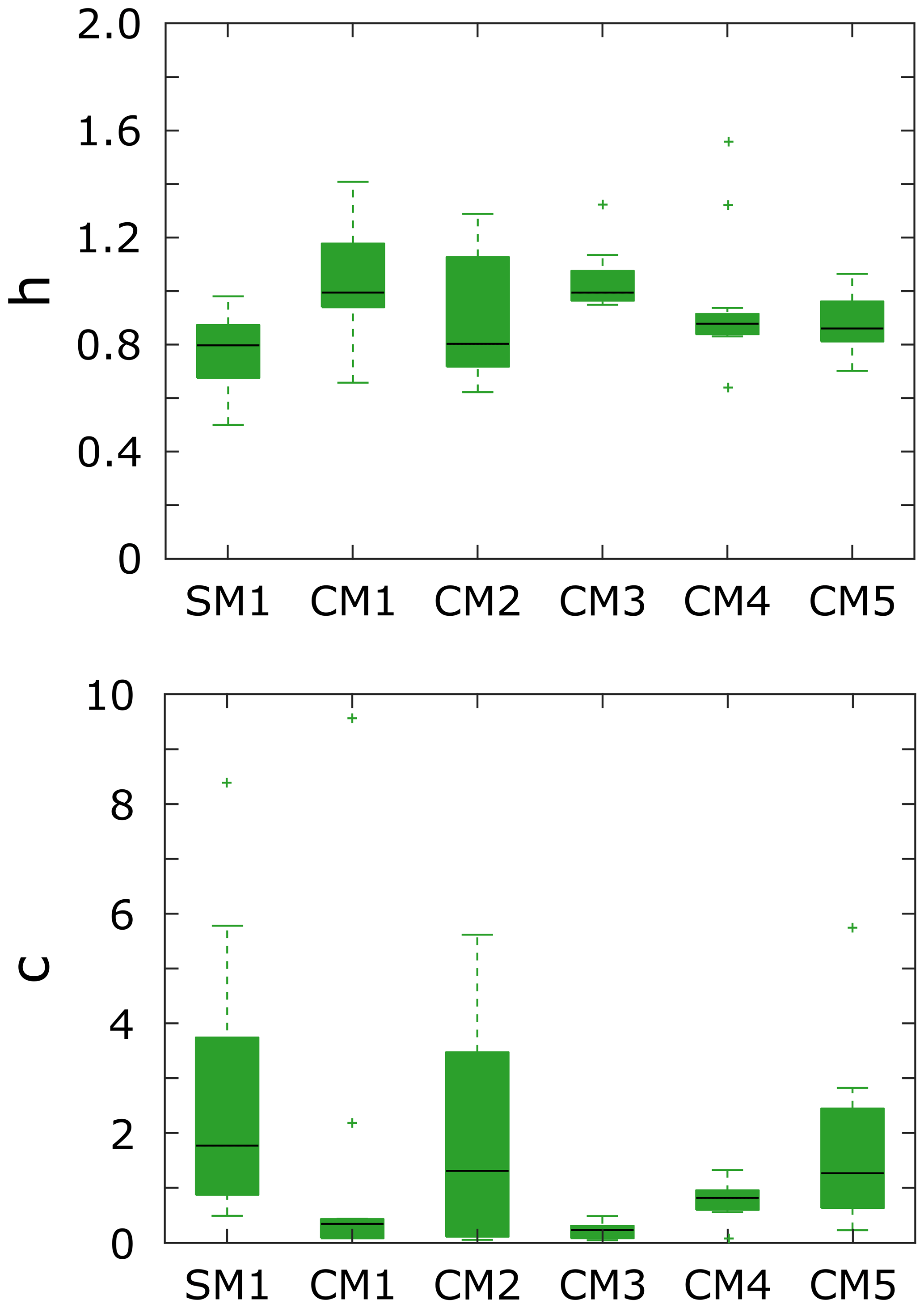
Figure 11Value distributions for h and c for Hack's law, as given in Eq. (13), in the models. The black lines indicate the median, while the bottom and top edges of the green box indicate the 25th and 75th percentiles, respectively. The green whiskers outside the box cover the data point at < 25th and > 75th percentiles that are not considered outliers, here indicated by green crosses.
4.5 Steepness and concavity index
We use the following metrics for quantifying erosion in both the laboratory and nature: ksn and θ. Both ksn and θ represent a 1:1 metric for a lab-to-nature comparison. θ is dimensionless, while ksn, whose dimensions are a function of a reference concavity θref, has been computed considering the length scaling factor h∗ = 10−5 (related to the strength of the granular materials) so that the values for A in analog models in Eq. (9) are in square meters. For calculating ksn in analog models (ksn_MOD) we assumed θref = 0.45, similar to studies on natural landscapes. We analyzed river profiles from phase II of the experiments because this phase is linked to the equilibrium of the system. In general, θ_MOD tends to be lower than 0.5, with the exception of CM2 and CM3, due to the straightening of river longitudinal profiles during the model run (Duvall, 2004; Whipple and Tucker, 1999). Despite the scattering of values for θ_MOD, SM1, CM2 and CM3 show average values higher than the other models, from 0.2 to 0.5 (for data between the 25th and 75th percentile). For ksn_MOD we found that values computed during phase II generally range between 10 and 140 m0.9 (Fig. 12). The values for ksn_MOD and θ_MOD do not allow for a unique discrimination between the types of erosion affecting the models in terms of detachment-limited erosion and transport-limited erosion (Tucker and Slingerland, 1997; Tucker and Whipple, 2002; Whipple and Tucker, 2002), but we consider it likely that experiments are often transport-limited rather than detachment-limited. The concavity index for detachment-limited streams is typically higher than for transport-limited streams (Brocard and Van der Beek, 2006; Whipple and Tucker, 2002), even if there is some evidence which suggests that this might not always be true (Gasparini, 1998; Massong and Montgomery, 2000; Tarboton et al., 1991). Of our models, CM2 and CM3 show the highest values for θ_MOD, while CM2 and SM1 show the highest values for ksn_MOD. Both ksn_MOD and θ_MOD (Fig. 12) are generally comparable with data coming from natural compilations (e.g., Kirby and Whipple, 2012) and studies on natural rivers in specific mountainous areas (Fig. 12). The matching of ksn and θ between models and nature supports future development and application of the analog materials tested in this study for modeling landscape evolution.
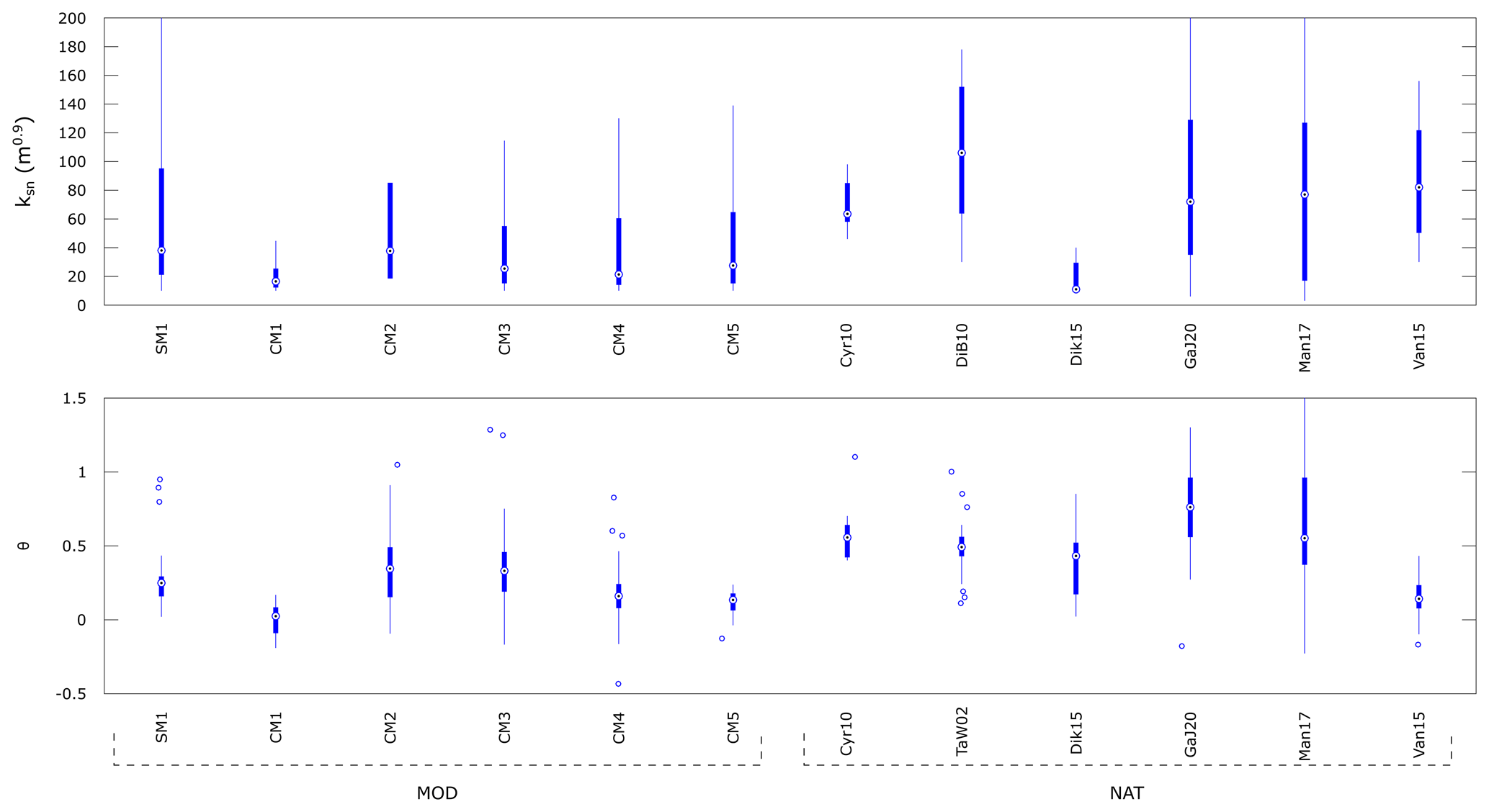
Figure 12Steepness (ksn) and concavity index (θ) in the experiments and in nature (field data). We use θref = 0.45 for computing ksn. The black dots indicate the median, while the bottom and top edges of the blue box indicate the 25th and 75th percentiles, respectively. The thin blue lines cover data < 25th and > 75th percentiles that are not considered outliers, and the outliers are indicated by the blue empty dots. Cyr10: Cyr et al., 2010; DiB10: DiBiase et al., 2010; TaW02: Tucker and Whipple, 2002; Dik15: Dikshit, 2015; GaJ20: Guha and Jain, 2020; Man17: Mandal et al., 2017; Van15: Vanacker et al., 2015.
We used mixes of water-saturated granular materials as analogs for the upper brittle crust, analyzing the role played by geometrical and physical properties in landscape evolution models. Our experimental results illustrate how small variations in the composition of an analog material can strongly affect the evolution of the geomorphological features and the mechanical response of the materials. In accordance with previous works, we find the main component of analog materials for landscape evolution models in SP, which is better if mixed with GM and PVC. We can now conclude the following.
- a.
Granular materials and mixes of them deform following the Mohr–Coulomb criterion.
- b.
Composite materials with smaller grain size distribution and higher grain size (order of 100–200 µm) do not allow for advection in valleys due to higher permeability. The sediment (mass) discharge rate is high, and the erosion happens quickly in time.
- c.
Composite materials with higher grain size distribution with particles of the order of tens of micrometers allow for both channel incision in valleys and diffusion on hillslopes.
- d.
Composite materials wherein the percentage of SP is higher than or equal to 50 wt % show a high number of channels but with very low incision. The discharge rate is extremely low, and erosion and incision affect the model less.
- e.
With respect to the other models, SM1 and CM2 show more branching and well-defined basins, while CM2 and CM3 show higher values for the concavity index.
The geomorphological observations carried out on the models presented here highlight how SM1, CM2 and CM3 show features most similar to natural prototypes. Increasing the SP concentration from 40 wt % to 50 wt % (CM2 and CM3, respectively) leads to straighter channels that are better defined. For models coupling tectonics and surface processes, the material used in SM1 is not likely to be adequate due to its deformational behavior (Sect. 4.2). The Hack's exponent in all models was higher than observed in nature, but SM1 and CM2 exhibited the lowest values. The concavity index for all models tended towards values lower than in nature, except for CM2 and CM3, which showed good agreement with nature. All these considerations suggest that the materials used in models CM2 and CM3 should be implemented for reproducing analog landscapes. Our findings are in agreement with previous works, and here we also quantified the differences between geomorphological indexes as a function of the composition of analog materials, giving a further constraint on the choice of materials. These mixes will be adopted in contexts of active tectonics in future works.
Digital images, topographic data from laser scans, scripts and raw data have been uploaded using GFZ Data Services and can be accessed through https://doi.org/10.5880/fidgeo.2020.021. They are published open-access in Reitano et al. (2020).
RR, CF, FF and FC proposed the original idea. RR, CF, FF and FC designed the experiments, and RR carried them out. RR and FC developed the codes for the model analysis that has been performed by all authors. Interpretation of results, writing, reviewing and editing were performed by all authors.
The authors declare that they have no conflict of interest.
We thank the editor Tom Coulthard, the associate editor Jean Braun, and the reviewers Fabien Graveleau and Michele Cooke, who helped improve this paper with their constructive comments. We would like to thank Diego Sebastiani, Anita Di Giulio, Maurizio Di Biase and Andrea Di Biase from the geotechnical laboratory at Università La Sapienza for the fundamental help and for the useful discussions. We thank Stéphane Dominguez for providing us with the materials that have been used for comparison to the materials presented in this paper. We thank Chiara Bazzucchi and Federica Sola for the help they provided. We also thank TPV Compound s.r.l. (Frosinone, Italy) for providing us with PVC powder and CNG Srl for their laboratories. In Fig. 9 we used the perceptually uniform color map Roma by Fabio Crameri. The grant to the Department of Science, Roma Tre University (MIUR-Italy Dipartimenti di Eccellenza, ARTICOLO 1, COMMI 314–337 LEGGE 232/2016), is gratefully acknowledged.
This paper was edited by Jean Braun and reviewed by Fabien Graveleau and Michele Cooke.
Babault, J., Bonnet, S., Crave, A., and Van Den Driessche, J.: Influence of piedmont sedimentation on erosion dynamics of an uplifting landscape: An experimental approach, Geology, 33, 301–304, https://doi.org/10.1130/G21095.1, 2005.
Batt, G. E. and Braun, J.: The tectonic evolution of the Southern Alps, New Zealand: Insights from fully thermally coupled dynamical modelling, Geophys. J. Int., 136, 403–420, https://doi.org/10.1046/j.1365-246X.1999.00730.x, 1999.
Beaumont, C., Fullsack, P., and Hamilton, J.: Erosional control of active compressional orogens, in: Thrust tectonics, Springer, Dordrecht, the Netherlands, 1–18, 1992.
Beaumont, C., Jamieson, R. A., Nguyen, M. H., and Lee, B.: Himalayan tectonics explained by extrusion of a low-viscosity crustal channel coupled to focused surface denudation, Nature, 414, 738–742, https://doi.org/10.1038/414738a, 2001.
Beaumont, C., Jamieson, R. A., Nguyen, M. H., and Medvedev, S.: Crustal channel flows: 1. Numerical models with applications to the tectonics of the Himalayan–Tibetan orogen, J. Geophys. Res.-Solid, 109, 1–29, https://doi.org/10.1029/2003JB002809, 2004.
Bonnet, S.: Shrinking and splitting of drainage basins in orogenic landscapes from the migration of themain drainage divide, Nat. Geosci., 2, 766–771, https://doi.org/10.1038/ngeo666, 2009.
Bonnet, S. and Crave, A.: Landscape response to climate change: Insights from experimental modeling and implications for tectonic versus climatic uplift of topography, Geol. Soc. Am. Bull., 31, 123–126, 2003.
Bonnet, S. and Crave, A.: Macroscale dynamics of experimental landscapes, Geol. Soc. Lond. Spec. Publ., 253, 327–339, https://doi.org/10.1144/gsl.sp.2006.253.01.17, 2006.
Braun, J. and Willett, S. D.: A very efficient O(n), implicit and parallel method to solve the stream power equation governing fluvial incision and landscape evolution, Geomorphology, 180–181, 170–179, https://doi.org/10.1016/j.geomorph.2012.10.008, 2013.
Braun, J. and Yamato, P.: Structural evolution of a three-dimensional, finite-width crustal wedge, Tectonophysics, 484, 181–192, https://doi.org/10.1016/j.tecto.2009.08.032, 2010.
Brocard, G. Y. and Van der Beek, P. A.: Influence of incision rate, rock strength, and bedload supply on bedrock river gradients and valley-flat widths: Field-based evidence and calibrations from western Alpine rivers (southeast France), Spec. Pap. Geol. Soc. Am., 398, 101–126, 2006.
Buiter, S. J. H.: A review of brittle compressional wedge models, Tectonophysics, 530–531, 1–17, https://doi.org/10.1016/j.tecto.2011.12.018, 2012.
Carman, P. C.: Determination of the specific surface of powders I. Transactions, J. Soc. Chem. Ind.-L., 57, 225–234, 1938.
Carman, P. C.: Flow of gases through porous media, Academic Press, New York, 1956.
Castelltort, S., Goren, L., Willett, S. D., Champagnac, J. D., Herman, F., and Braun, J.: River drainage patterns in the New Zealand Alps primarily controlled by plate tectonic strain, Nat. Geosci., 5, 744–748, https://doi.org/10.1038/ngeo1582, 2012.
Castillo, M., Muñoz-Salinas, E., and Ferrari, L.: Response of a landscape to tectonics using channel steepness indices (ksn) and OSL: A case of study from the Jalisco Block, Western Mexico, Geomorphology, 221, 204–214, https://doi.org/10.1016/j.geomorph.2014.06.017, 2014.
Collignon, M., Kaus, B. J. P., May, D. A., and Fernandez, N.: Influences of surface processes on fold growth during 3-D detachment folding, Geochem. Geophy. Geosy., 15, 3281–3303, https://doi.org/10.1002/2014GC005450, 2014.
Cruz, L., Teyssier, C., Perg, L., Take, A., and Fayon, A.: Deformation, exhumation, and topography of experimental doubly-vergent orogenic wedges subjected to asymmetric erosion, J. Struct. Geol., 30, 98–115, https://doi.org/10.1016/j.jsg.2007.10.003, 2008.
Cyr, A. J., Granger, D. E., Olivetti, V., and Molin, P.: Quantifying rock uplift rates using channel steepness and cosmogenic nuclide-determined erosion rates: Examples from northern and southern Italy, Lithosphere, 2, 188–198, https://doi.org/10.1130/L96.1, 2010.
Cyr, A. J., Granger, D. E., Olivetti, V., and Molin, P.: Distinguishing between tectonic and lithologic controls on bedrock channel longitudinal profiles using cosmogenic 10Be erosion rates and channel steepness index, Geomorphology, 209, 27–38, https://doi.org/10.1016/j.geomorph.2013.12.010, 2014.
Davis, D., Suppe, J., and Dahlen, F. A.: Mechanics of Fold-and-Thrust Belts and Accretionary Wedges, J. Geophys. Res., 88, 1153–1172, https://doi.org/10.1029/JB089iB12p10087, 1983.
Davy, P. and Cobbold, P. R.: Experiments on shortening of a 4-layer model of the continental lithosphere, Tectonophysics, 188, 1–25, https://doi.org/10.1016/0040-1951(91)90311-F, 1991.
DiBiase, R. A., Whipple, K. X., Heimsath, A. M., and Ouimet, W. B.: Landscape form and millennial erosion rates in the San Gabriel Mountains, CA, Earth Planet. Sc. Lett., 289, 134–144, https://doi.org/10.1016/j.epsl.2009.10.036, 2010.
Dikshit, V. M.: Steepness Index Derived Areas of Differential Rock Uplift Rates in the Lanja Region From Southern Konkan Coastal Belt, Maharashtra, J. Emerg. Technol. Innov. Res., 2, 221–230, 2015.
Dodds, P. S. and Rothman, D. H.: Scaling, universality, and geomorphology, Annu. Rev. Earth Planet. Sci., 28, 571–610, https://doi.org/10.1146/annurev.earth.28.1.571, 2000.
Duvall, A.: Tectonic and lithologic controls on bedrock channel profiles and processes in coastal California, J. Geophys. Res., 109, 1–18, https://doi.org/10.1029/2003jf000086, 2004.
Duvall, A. R. and Tucker, G. E.: Dynamic Ridges and Valleys in a Strike-Slip Environment, J. Geophys. Res.-Earth, 120, 2016–2026, https://doi.org/10.1002/2015JF003618, 2015.
Flint, J. J.: Stream Gradient as a Function of Order, Magnitude, and Discharge, Water Resour. Res., 10, 969–973, 1974.
Gasparini, N. M.: Erosion and deposition of multiple grain sizes in a landscape evolution model, MS thesis, Massachusetts Institute of Technology, Cambridge, 105 pp., 1998.
Goren, L., Castelltort, S., and Klinger, Y.: Modes and rates of horizontal deformation from rotated river basins: Application to the Dead Sea fault system in Lebanon, Geology, 43, 843–846, https://doi.org/10.1130/G36841.1, 2015.
Graveleau, F.: Interactions Tectonique, Erosion , Sédimentation dans les avant-pays de chaînes?: Modélisation analogique et étude des piémonts de l'est du Tian Shan (Asie centrale), Université Montpellier II, Montpellier, 2008.
Graveleau, F. and Dominguez, S.: Analogue modelling of the interaction between tectonics, erosion and sedimentation in foreland thrust belts, C. R. Geosci., 340, 324–333, https://doi.org/10.1016/j.crte.2008.01.005, 2008.
Graveleau, F., Hurtrez, J., Dominguez, S., and Malavieille, J.: A new experimental material for modeling relief dynamics and interactions between tectonics and surface processes, Tectonophysics, 513, 68–87, https://doi.org/10.1016/j.tecto.2011.09.029, 2011.
Graveleau, F., Malavieille, J., and Dominguez, S.: Experimental modelling of orogenic wedges: A review, Tectonophysics, 538–540, 1–66, https://doi.org/10.1016/j.tecto.2012.01.027, 2012.
Graveleau, F., Strak, V., Dominguez, S., Malavieille, J., Chatton, M., Manighetti, I., and Petit, C.: Experimental modelling of tectonics-erosion-sedimentation interactions in compressional, extensional, and strike-slip settings, Geomorphology, 244, 146–168, https://doi.org/10.1016/j.geomorph.2015.02.011, 2015.
Guerit, L., Dominguez, S., Malavieille, J., and Castelltort, S.: Deformation of an experimental drainage network in oblique collision, Tectonophysics, 693, 210–222, https://doi.org/10.1016/j.tecto.2016.04.016, 2016.
Guha, S. and Jain, V.: Role of inherent geological and climatic characteristics on landscape variability in the tectonically passive Western Ghat, India, Geomorphology, 350, 106840, https://doi.org/10.1016/j.geomorph.2019.106840, 2020.
Hack, J. T.: Studies of longitudinal profiles in Virginia and Maryland, no. 294-B in US Geol. Survey Prof. Papers, US Government Printing Office, Washington, D.C., https://doi.org/10.3133/pp294B, 1957.
Hasbargen, L. E. and Paola, C.: Landscape instability in an experimental drainage basin, Geology, 28, 1067–1070, https://doi.org/10.1130/0091-7613(2000)028<1067:LIIAED>2.3.CO;2, 2000.
Hoth, S., Adam, J., Kukowski, N., and Oncken, O.: Influence of erosion on the kinematics of bivergent orogens: Results from scaled sandbox simulations, Geol. S. Am. S., 398(303), 201–225, https://doi.org/10.1130/2006.2398(12), 2006.
Howard, A. D.: A detachment limited model of drainage basin evolution, Water Resour. Res., 30, 2261–2285, https://doi.org/10.1029/94WR00757, 1994.
Howard, A. D., Dietrich, W. E., and Seidl, M. A.: Modeling fluvial erosion on regional to continental scale, J. Geophys. Res., 99, 13971–13986, 1994.
Hubbert, M. K.: Theory of Scale Models as Applied to the Study of Geologic Structures, Geol. Soc. Am. Bull., 48, 1459–1520, 1937.
Jamieson, R. A., Beaumont, C., Medvedev, S., and Nguyen, M. H.: Crustal channel flows: 2. Numerical models with implications for metamorphism in the Himalayan–Tibetan orogen, J. Geophys. Res.-Solid, 109, 1–24, https://doi.org/10.1029/2003JB002811, 2004.
Kirby, E. and Whipple, K. X.: Quantifying differential rock-uplift rates via stream profile analysis, Geology, 29, 415–418, https://doi.org/10.1130/0091-7613(2001)029<0415:QDRURV>2.0.CO;2, 2001.
Kirby, E. and Whipple, K. X.: Expression of active tectonics in erosional landscapes, J. Struct. Geol., 44, 54–75, https://doi.org/10.1016/j.jsg.2012.07.009, 2012.
Konstantinovskaya, E. and Malavieille, J.: Thrust wedges with décollement levels and syntectonic erosion: A view from analog models, Tectonophysics, 502, 336–350, https://doi.org/10.1016/j.tecto.2011.01.020, 2011.
Kozeny, J.: Ueber kapillare Leitung des Wassers im Boden [Capillary flow of water in the soil], Sitzungsberichte der Akademie der Wissenschaften in Wien, 136, 271–306, 1927.
Krantz, R. W.: Measurements of friction coefficients and cohesion for faulting and fault reactivation in laboratory models using sand and sand mixtures, Tectonophysics, 188, 203–207, https://doi.org/10.1016/0040-1951(91)90323-K, 1991.
Lague, D., Crave, A., and Davy, P.: Laboratory experiments simulating the geomorphic response to tectonic uplift, J. Geophys. Res.-Solid, 108, ETG 3-1–ETG 3-20, https://doi.org/10.1029/2002JB001785, 2003.
Lallemand, S. E., Schnurle, P., and Malavieille, J.: Coulomb theory applied to accretionary and nonaccretionary wedges: Possible causes for tectonic erosion and/or frontal accretion, J. Geophys. Res., 99, 12033–12055, 1994.
Lohrmann, J., Kukowski, N., Adam, J., and Oncken, O.: The impact of analogue material properties on the geometry, kinematics, and dynamics of convergent sand wedges, J. Struct. Geol., 25, 1691–1711, https://doi.org/10.1016/S0191-8141(03)00005-1, 2003.
Malavieille, J., Larroque, C., and Calassou, S.: Modélisation expérimentale des relations tectonique/sédimentation entre bassin avant-arc et prisme d'accrétion, Comptes Rendus de l'Académie des Sciences, Paris, 1131–1137, 1993.
Mandal, S. K., Burg, J. P., and Haghipour, N.: Geomorphic fluvial markers reveal transient landscape evolution in tectonically quiescent southern Peninsular India, Geol. J., 52, 681–702, https://doi.org/10.1002/gj.2833, 2017.
Massong, T. M. and Montgomery, D. R.: Influence of sediment supply, lithology, and wood debris on the distribution of bedrock and alluvial channels, Geol. Soc. Am. Bull., 112, 591–599, https://doi.org/10.1130/0016-7606(2000)112<591:IOSSLA>2.0.CO;2, 2000.
Montanari, D., Agostini, A., Bonini, M., Corti, G., and Del Ventisette, C.: The use of empirical methods for testing granular materials in analogue modelling, Materials, 10, 1–18, https://doi.org/10.3390/ma10060635, 2017.
Mulugeta, G. and Koyi, H.: Three-dimensional geometry and kinematics of experimental piggyback thrusting, Geology, 15, 1052–1056, https://doi.org/10.1130/0091-7613(1987)15<1052:TGAKOE>2.0.CO;2, 1987.
Ouchi, S.: Effects of uplift on the development of experimental erosion landform generated by artificial rainfall, Geomorphology, 127, 88–98, https://doi.org/10.1016/j.geomorph.2010.12.009, 2011.
Panien, M., Schreurs, G., and Pfiffner, A.: Mechanical behaviour of granular materials used in analogue modelling: insights from grain characterisation, ring-shear tests and analogue experiments, J. Struct. Geol., 28, 1710–1724, https://doi.org/10.1016/j.jsg.2006.05.004, 2006.
Paola, C., Straub, K., Mohrig, D., and Reinhardt, L.: The “unreasonable effectiveness” of stratigraphic and geomorphic experiments, Earth-Sci. Rev., 97, 1–43, https://doi.org/10.1016/j.earscirev.2009.05.003, 2009.
Pederson, J. L. and Tressler, C.: Colorado River long-profile metrics, knickzones and their meaning, Earth Planet. Sc. Lett., 345–348, 171–179, https://doi.org/10.1016/j.epsl.2012.06.047, 2012.
Persson, K. S., Garcia-Castellanos, D., and Sokoutis, D.: River transport effects on compressional belts: First results from an integrated analogue-numerical model, J. Geophys. Res.-Solid, 109, 1–11, https://doi.org/10.1029/2002JB002274, 2004.
Ramberg, H.: Gravity, deformation and the earth's crust: in theory, experiments and geological application, Academic Press, New York, 1981.
Reber, J. E., Cooke, M. L., and Dooley, T. P.: What model material to use? A Review on rock analogs for structural geology and tectonics, Earth-Sci. Rev., 202, 103107, https://doi.org/10.1016/j.earscirev.2020.103107, 2020.
Reitano, R., Faccenna, C., Funiciello, F., Corbi, F., and Willett, S. D.: Experimental data of analogue landscape evolution models, GFZ Data Services, https://doi.org/10.5880/fidgeo.2020.021, 2020.
Rigon, R., Rodriguez-Iturbe, I., Maritan, A., Giacometti, A., Tarboton, D. G., and Rinaldo, A.: On Hack's law, Water Resour. Res., 32, 3367–3374, 1996.
Ritter, M. C., Santimano, T., Rosenau, M., Leever, K., and Oncken, O.: Sandbox rheometry: Co-evolution of stress and strain in Riedel- and Critical Wedge-experiments, Tectonophysics, 722, 400–409, https://doi.org/10.1016/j.tecto.2017.11.018, 2018.
Rossi, D. and Storti, F.: New artificial granular materials for analogue laboratory experiments: Aluminium and siliceous microspheres, J. Struct. Geol., 25, 1893–1899, https://doi.org/10.1016/S0191-8141(03)00041-5, 2003.
Schellart, W. P.: Shear test results for cohesion and friction coefficients for different granular materials: Scaling implications for their usage in analogue modelling, Tectonophysics, 324, 1–16, https://doi.org/10.1016/S0040-1951(00)00111-6, 2000.
Schreurs, G., Hänni, R., and Vock, P.: Four-dimensional analysis of analog models: Experiments on transfer zones in fold and thrust belts, Memoir Geol. Soc. Am., 193, 179–190, https://doi.org/10.1130/0-8137-1193-2.179, 2001.
Schreurs, G., Buiter, S. J. H., Boutelier, D., Corti, G., Costa, E., Cruden, A. R., Daniel, J.-M., Hoth, S., Koyi, H. A., Kukowski, N., Lohrmann, J., Ravaglia, A., Schlische, R. W., Withjack, M. O., Yamada, Y., Cavozzi, C., Del Ventisette, C., Brady, J. A. E., Hoffmann-Rothe, A., Mengus, J.-M., Montanari, D., and Nilforoushan, F.: Analogue benchmarks of shortening and extension experiments, Geol. Soc. Lond. Spec. Publ., 253, 1–27, https://doi.org/10.1144/GSL.SP.2006.253.01.01, 2006.
Schreurs, G., Buiter, S. J. H., Boutelier, J., Burberry, C., Callot, J. P., Cavozzi, C., Cerca, M., Chen, J. H., Cristallini, E., Cruden, A. R., Cruz, L., Daniel, J. M., Da Poian, G., Garcia, V. H., Gomes, C. J. S., Grall, C., Guillot, Y., Guzmán, C., Hidayah, T. N., Hilley, G., Klinkmüller, M., Koyi, H. A., Lu, C. Y., Maillot, B., Meriaux, C., Nilfouroushan, F., Pan, C. C., Pillot, D., Portillo, R., Rosenau, M., Schellart, W. P., Schlische, R. W., Take, A., Vendeville, B., Vergnaud, M., Vettori, M., Wang, S. H., Withjack, M. O., Yagupsky, D., and Yamada, Y.: Benchmarking analogue models of brittle thrust wedges, J. Struct. Geol., 92, 116–139, https://doi.org/10.1016/j.jsg.2016.03.005, 2016.
Schumm, S. A. and Parker, R. S.: Implications of Complex Response of Drainage Systems for Quaternary Alluvial Stratigraphy, Nat. Phys. Sci., 243, 99–100, https://doi.org/10.1038/physci243099a0, 1973.
Schumm, S. A. and Rea, D. K.: Sediment yields from disturbed earth systems, Geology, 23, 391–394, https://doi.org/10.1130/0091-7613(1995)023<0391:syfdes>2.3.co;2, 1995.
Schwanghart, W. and Scherler, D.: Short Communication: TopoToolbox 2 – MATLAB-based software for topographic analysis and modeling in Earth surface sciences, Earth Surf. Dynam., 2, 1–7, https://doi.org/10.5194/esurf-2-1-2014, 2014.
Sembroni, A., Molin, P., Pazzaglia, F. J., Faccenna, C., and Abebe, B.: Evolution of continental-scale drainage in response to mantle dynamics and surface processes: An example from the Ethiopian Highlands, Geomorphology, 261, 12–29, https://doi.org/10.1016/j.geomorph.2016.02.022, 2016.
Singh, A., Reinhardt, L., and Foufoula-Georgiou, E.: Landscape reorganization under changing climatic forcing: Results from an experimental landscape, Water Resour. Res., 51, 4320–4337, https://doi.org/10.1002/2015WR017161, 2015.
Storti, F. and McClay, K.: Influence of syntectonic sedimentation on thrust wedges in analogue models, Geology, 23, 999–1002, https://doi.org/10.1130/0091-7613(1995)023<0999:IOSSOT>2.3.CO;2, 1995.
Storti, F., Salvini, F., and McClay, K.: Synchronous and velocity-partitioned thrusting and thrust polarity reversal in experimentally produced, doubly-vergent thrust wedges: Implications for natural orogens, Tectonics, 19, 378–396, https://doi.org/10.1029/1998TC001079, 2000.
Strak, V., Dominguez, S., Petit, C., Meyer, B., and Loget, N.: Interaction between normal fault slip and erosion on relief evolution: Insights from experimental modelling, Tectonophysics, 513, 1–19, https://doi.org/10.1016/j.tecto.2011.10.005, 2011.
Tarboton, D. G., Bras, R. L., and Rodriguez-Iturbe, I.: On the extraction of channel networks from digital elevation data, Hydrol. Process., 5, 81–100, https://doi.org/10.1002/hyp.3360050107, 1991.
Tejedor, A., Singh, A., Zaliapin, I., Densmore, A. L., and Foufoula-Georgiou, E.: Scale-dependent erosional patterns in steady-state and transient-state landscapes, Sci. Adv., 3, 1–8, https://doi.org/10.1126/sciadv.1701683, 2017.
Tucker, G. E. and Slingerland, R.: Drainage basin responses to climate change, Water Resour. Res., 33, 2031–2047, https://doi.org/10.1029/97WR00409, 1997.
Tucker, G. E. and Whipple, K. X.: Topographic outcomes predicted by stream erosion models: Sensitivity analysis and intermodel comparison, J. Geophys. Res.-Solid, 107, ETG 1-1–ETG 1-16, https://doi.org/10.1029/2001JB000162, 2002.
Ueda, K., Willett, S. D., Gerya, T., and Ruh, J.: Geomorphological-thermo-mechanical modeling: Application to orogenic wedge dynamics, Tectonophysics, 659, 12–30, https://doi.org/10.1016/j.tecto.2015.08.001, 2015.
Vanacker, V., von Blanckenburg, F., Govers, G., Molina, A., Campforts, B., and Kubik, P. W.: Transient river response, captured by channel steepness and its concavity, Geomorphology, 228, 234–243, https://doi.org/10.1016/j.geomorph.2014.09.013, 2015.
Viaplana-Muzas, M., Babault, J., Dominguez, S., Van Den Driessche, J., and Legrand, X.: Drainage network evolution and patterns of sedimentation in an experimental wedge, Tectonophysics, 664, 109–124, https://doi.org/10.1016/j.tecto.2015.09.007, 2015.
Viaplana-Muzas, M., Babault, J., Dominguez, S., Van Den Driessche, J., and Legrand, X.: Modelling of drainage dynamics influence on sediment routing system in a fold-and-thrust belt, Basin Res., 31, 290–310, https://doi.org/10.1111/bre.12321, 2019.
Whipple, K. X. and Meade, B. J.: Controls on the strength of coupling among climate, erosion, and deformation in two-sided, frictional orogenic wedges at steady state, J. Geophys. Res.-Earth, 109, 1–24, https://doi.org/10.1029/2003JF000019, 2004.
Whipple, K. X. and Tucker, G. E.: Dynamics of the stream-power river incision model: Implications for height limits of mountain ranges, landscape response timescales, and research needs, J. Geophys. Res., 104, 17661–17674, 1999.
Whipple, K. X. and Tucker, G. E.: Implications of sediment-flux-dependent river incision models for landscape evolution, J. Geophys. Res., 107, 2039, https://doi.org/10.1029/2000JB000044, 2002.
Whipple, K. X., Kirby, E., and Brocklehurst, S. H.: Geomorphic limits to climate-induced increases in topographic relief, Nature, 401, 39–43, https://doi.org/10.1038/43375, 1999.
Willett, S. D.: Orogeny and orography: The effects of erosion on the structure of mountain belts, J. Geophys. Res.-Solid, 104, 28957–28981, https://doi.org/10.1029/1999JB900248, 1999.
Willett, S. D., Beaumont, C., and Fullsack, P.: Mechanical Model for doubly vergent compressional orogens, Geology, 21, 371–374, https://doi.org/10.1130/0091-7613(1993)021<0371:MMFTTO>2.3.CO;2, 1993.