the Creative Commons Attribution 4.0 License.
the Creative Commons Attribution 4.0 License.
 | 26 Aug 2021
Effect of rock uplift and Milankovitch timescale variations in precipitation and vegetation cover on catchment erosion rates
Hemanti Sharma
Todd A. Ehlers
Christoph Glotzbach
Manuel Schmid
Katja Tielbörger
Catchment erosion and sedimentation are influenced by variations in the rates of rock uplift (tectonics) and periodic fluctuations in climate and vegetation cover. This study focuses on quantifying the effects of changing climate and vegetation on erosion and sedimentation over distinct climate–vegetation settings by applying the Landlab–SPACE landscape evolution model. As catchment evolution is subjected to tectonic and climate forcings at millennial to million-year timescales, the simulations are performed for different tectonic scenarios and periodicities in climate–vegetation change. We present a series of generalized experiments that explore the sensitivity of catchment hillslope and fluvial erosion as well as sedimentation for different rock uplift rates (0.05, 0.1, 0.2 mm a−1) and Milankovitch climate periodicities (23, 41, and 100 kyr). Model inputs were parameterized for two different climate and vegetation conditions at two sites in the Chilean Coastal Cordillera at ∼26∘ S (arid and sparsely vegetated) and ∼33∘ S (Mediterranean). For each setting, steady-state topographies were produced for each uplift rate before introducing periodic variations in precipitation and vegetation cover. Following this, the sensitivity of these landscapes was analyzed for 3 Myr in a transient state. Results suggest that regardless of the uplift rate, transients in precipitation and vegetation cover resulted in transients in erosion rates in the direction of change in precipitation and vegetation. The transients in sedimentation were observed to be in the opposite direction of change in the precipitation and vegetation cover, with phase lags of ∼1.5–2.5 kyr. These phase lags can be attributed to the changes in plant functional type (PFT) distribution induced by the changes in climate and the regolith production rate. These effects are most pronounced over longer-period changes (100 kyr) and higher rock uplift rates (0.2 mm yr−1). This holds true for both the vegetation and climate settings considered. Furthermore, transient changes in catchment erosion due to varying vegetation and precipitation were between ∼35 % and 110 % of the background (rock uplift) rate and would be measurable with commonly used techniques (e.g., sediment flux histories, cosmogenic nuclides). Taken together, we find that vegetation-dependent erosion and sedimentation are influenced by Milankovitch timescale changes in climate but that these transient changes are superimposed upon tectonically driven rates of rock uplift.
- Article
(4286 KB) - Full-text XML
- BibTeX
- EndNote


The pioneering work of Grove Karl Gilbert (Gilbert, 1877) highlighted the fact that surface uplift, climate, and biota (amongst other things) jointly influence catchment-scale rates of weathering and erosion. In recent decades a wide range of studies have built upon these concepts and quantified different ways in which climate, tectonics, or vegetation cover influence rates of erosion and sedimentation. For example, recent work highlights the fact that denser vegetation and lower precipitation both decrease erosion (Alonso et al., 2006; Bonnet and Crave, 2003; Huntley et al., 2013; McPhillips et al., 2013; Miller et al., 2013; Perron, 2017; Schaller et al., 2018; Starke et al., 2020; Tucker, 2004). In addition, periodic changes in climate (such as changes driven by Milankovitch timescale orbital variations) have also been recognized as influencing rates of catchment erosion and sedimentation (Braun et al., 2015; Hancock and Anderson, 2002; Hyun et al., 2005; Schaller et al., 2004), although our ability to measure orbital-timescale-induced erosional changes can be challenging (e.g., Schaller and Ehlers, 2006; Whipple, 2009). Several studies have also documented how the combined effects of either climate and vegetation change or variable rates of rock uplift and climate change (including glaciation) impact catchment-scale processes (Herman et al., 2010; Mishra et al., 2019; Schmid et al., 2018; Tucker, 2004; Yanites and Ehlers, 2012). Taken together, previous studies have found that the long-term development of topography (such as over million-year timescales) is in many situations sensitive to the tectonic, climate, and vegetation history of the region and that competing effects of different coeval processes (e.g., climate change and tectonics) exist but are not well understood.
Quantification of climate, vegetation, and tectonic effects on catchment erosion is challenging because these processes are confounded and can, if coupled, have opposing effects on erosion and/or sedimentation. For example, precipitation has both direct (positive) and indirect effects on erosion that operate via vegetation cover. Namely, plants require water to grow and survive, and vegetation cover is usually positively affected by precipitation both on a global scale (i.e., when comparing biomes across latitudinal gradients) and on a regional or local scale (e.g., Huxman et al., 2004; Sala et al., 1988; Zhang et al., 2016). Though vegetation cover is also influenced by temperature, seasonality, and many other abiotic factors such as soil type and thickness, the positive relationship of biomass and cover with water availability is rather general. For example, in dry ecosystems such as hot deserts and Mediterranean systems, vegetation cover is primarily limited by water availability and is therefore very low. As precipitation increases, vegetation cover increases rapidly, although water availability can still be the limiting factor in addition to other factors (Breckle, 2002). In temperate systems, wherein water is abundant and soils are well developed, plant growth is primarily limited by low winter temperatures. Overall, the relationship between precipitation and vegetation cover follows a saturation curve with large sensitivity (e.g., measured as rain use efficiency – RUE) to precipitation in arid to Mediterranean systems and low sensitivity in temperate or tropical systems (Gerten et al., 2008; Huxman et al., 2004; Yang et al., 2008; Knapp et al., 2017).
Previous modeling and observational studies have made significant progress in understanding the interactions between surface processes and either climate (Dixon et al., 2009; Routschek et al., 2014; Seybold et al., 2017; Slater and Singer, 2013), vegetation (Acosta et al., 2015; Amundson et al., 2015; Istanbulluoglu and Bras, 2005), or coupled climate–vegetation dynamics (Dosseto et al., 2010; Jeffery et al., 2014; Mishra et al., 2019; Schmid et al., 2018). Over geologic (millennial to million-year) timescales, observational studies of these interactions are impossible (or require proxy data) and numerical modeling approaches provide a means to explore interactions between climate, vegetation, tectonics, and topography. The first observational study of this kind suggested that high MAP (mean annual precipitation) is associated with denser vegetation, hence resulting in lower erosion rates (Davy and Lague, 2009). One of the first numerical modeling studies implementing a vegetation–erosion coupling was conducted by Collins et al. (2004). This study was followed by work from Istanbulluoglu and Bras (2006), which quantified the effect of vegetation on landscape relief and drainage formation. More recently, work by Schmid et al. (2018) included the effects of transient climate and vegetation coupled with a landscape evolution model to predict topographic and erosional variations over millennial to million-year timescales. However, Schmid et al. (2018) presented a simplified approach to consider hillslope and detachment-limited fluvial erosion and only considered a homogeneous substrate. Other studies have documented the fact that sediment or bedrock erosion by rivers is not dominated purely by detachment-limited (Howard, 1994) or transport-limited fluvial erosion (Willgoose et al., 1991). Rather, it often involves a combination of or transition between the two conditions (e.g., Pelletier, 2012). Given this, treatment of bedrock erosion and sediment transport for mixed bedrock–alluvial streambeds provides a more realistic framework for understanding the influence of climate, vegetation, and tectonic processes on topographic development. Recent work (Shobe et al., 2017) presented an additional component (SPACE) to the Landlab surface process model. SPACE allows for the simulation of mixed detachment–transport-limited fluvial processes, including separate layers for bedrock and loose sediment. Finally, the sensitivity of topography to different rock uplift rates in variable climate–vegetation settings has not yet been investigated. The combined interactions of tectonics (rock uplift) and variable climate and vegetation warrant investigation given the significant influence of rock uplift on mean elevation, erosion rates and river channel profiles (Kirby and Whipple, 2012; Turowski et al., 2006), and hillslopes.
In this study, we complement previous work and investigate the transient landscape response for mixed bedrock–alluvial systems. We do this for different rates of rock uplift and periodic changes (Milankovitch cycles) in precipitation and vegetation. Our focus is on erosion and sedimentation changes occurring over millennial to million-year timescales. Sub-annual to decadal-scale changes are beyond the scope of this study. More specifically, this study evaluates the following two hypotheses: first, if vegetation cover and climate vary on Milankovitch timescales, then any increases or decreases in catchment erosion will be more pronounced over longer (e.g., 100 kyr) rather than shorter (e.g., 21 kyr) periodicities due to the longer duration of change imposed. Second, if increasing rates of tectonic uplift cause increases in catchment erosion rates, then any periodic variations in climate and vegetation cover will be muted (lower amplitude) at higher uplift rates because the effect of rock uplift on erosion will outweigh climate and vegetation change effects. Given the complexity of this problem, we investigate these hypotheses through numerical landscape evolution modeling using a stepwise increase in model complexity whereby the contributions of individual processes (i.e., climate, vegetation, or tectonics) are identified separately before looking into the fully coupled system and resulting interactions. We apply a two-dimensional coupled detachment–transport-limited landscape evolution model for fluvial processes. In addition, hillslope diffusion (Johnstone and Hilley, 2014) and weathering and soil production (Ahnert, 1977) processes are considered. Although this study is primarily focused on documenting the predicted sensitivity of catchments to variations in tectonics, climate, and vegetation change, we have tuned our model setup to the conditions along the Chilean Coastal Cordillera (Fig. 1), which features a similar tectonic setting but an extreme climate and ecological gradient. This was done to provide realistic parameterizations for vegetation cover and precipitation in different ecological settings. This area is also part of the German–Chilean priority research program, EarthShape: Earth Surface Shaping by Biota (https://esdynamics.geo.uni-tuebingen.de/earthshape/index.php?id=129, last access: 15 January 2021), for which extensive research is ongoing.
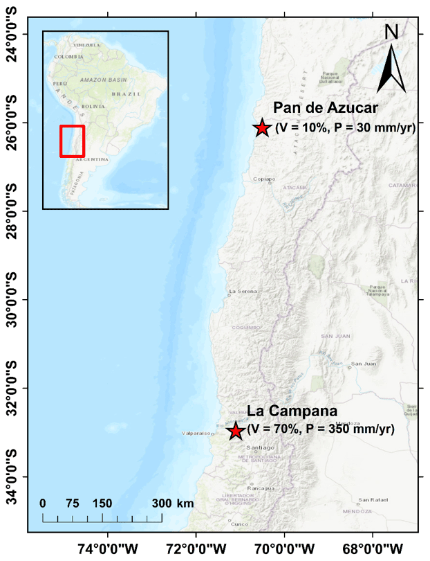
Figure 1The representative study areas in the Chilean Coastal Cordillera used for the model setup. The model parameters were loosely tuned to the climate and vegetation conditions in these areas (Schmid et al., 2018). The Pan de Azucar area in the north neighbors the Atacama Desert and has sparse vegetation cover (10 %) and an arid climate (30 mm yr−1). The La Campana area in south has a Mediterranean climate and ecosystem with more abundant vegetation (70 %) and precipitation (350 mm yr−1). These two study areas are part of the German EarthShape priority research program (https://esdynamics.geo.uni-tuebingen.de/earthshape/index.php?id=129, last access: 15 January 2021).
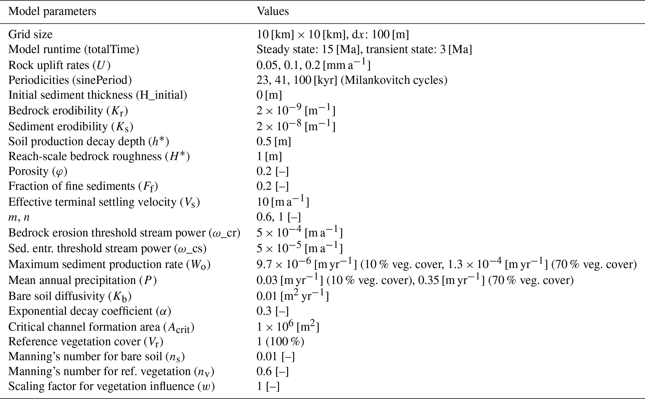
We apply the landscape evolution model, Landlab (Hobley et al., 2017), using the SPACE 1.0 module of Shobe et al. (2017) for detachment- vs. transport-limited fluvial processes. The Landlab–SPACE programs were modified for vegetation-dependent hillslope and fluvial erosion using the approach of Schmid et al. (2018). In general, the geomorphic processes considered involve weathering and regolith production calibrated to the Chilean Coastal Cordillera observations of Schaller et al. (2018), vegetation-dependent coupled detachment–transport-limited fluvial erosion, and depth-dependent hillslope diffusion. The model parameters (i.e., bedrock and sediment erodibility and diffusion coefficient) in the simulations are based on those of Schmid et al. (2018). A detailed explanation of the weathering, erosion, sediment transport, and deposition processes is provided in Appendix A, and a summary of model parameters used is given in Table A1.
2.1 Model setup and scenarios considered
The model consists of a 10 km by 10 km rectangular grid with 100 m node spacing (Fig. 2a), with a total domain area of 100 km2. We conducted generalized simulations that are loosely tuned to the climate and vegetation conditions in two areas in the Chilean Coastal Cordillera (Fig. 1), which have predominantly granitoid lithology (van Dongen et al., 2019; Kojima et al., 2017; Oeser et al., 2018; Rossel et al., 2018). These areas exhibit a large climate and vegetation gradient ranging from an arid climate (MAP: 30 mm) and sparse vegetation (10 %) in Pan de Azucar National Park to a wetter Mediterranean climate (MAP: 35 cm) with more abundant vegetation (70 %) in La Campana National Park.
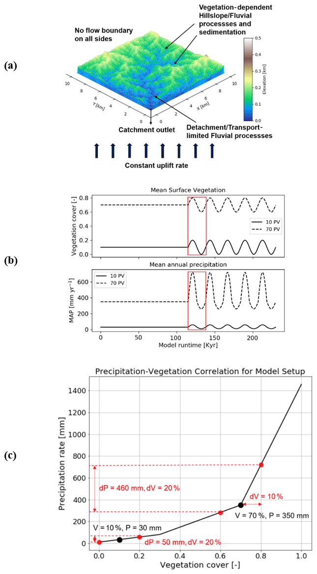
Figure 2Model geometry as well as climate and vegetation forcings used in this study. (a) A simple representation of the model setup with a square grid, and catchment outlet in the lower left corner. (b) Graphical representation of the magnitude and pattern of fluctuations imposed on vegetation (top) and precipitation (bottom) during the transient state of the model. Red rectangles represent one cycle, whose effects are discussed in detail. (c) Graphical representation of precipitation and vegetation cover correlation from the Chilean study areas used as the empirical basis for how precipitation rates vary for ±10 % changes in vegetation cover (Schmid et al., 2018).
Bedrock elevation and sediment cover thickness are considered to be separate layers to quantify simultaneous bedrock erosion and sediment entrainment across the model domain. Simulations were conducted for 15 Myr to generate a steady-state topography with the mean values of precipitation and vegetation cover for the two study areas. The rates of rock uplift are kept constant during the steady-state simulations and subsequently in the transient stage with oscillating vegetation cover and precipitation. After the development of a steady-state topography, transient forcings in vegetation cover and mean annual precipitation (MAP) (Fig. 2b) were introduced for 3 Myr. Vegetation cover varied by ±10 % around the mean value used to develop the steady-state topography. The 10 % vegetation cover variation is based on the dynamic vegetation modeling results of Werner et al. (2018) for the Chilean Coastal Cordillera. They found that from the Last Glacial Maximum to the present, vegetation cover in the region varied by ∼10 %. The periodicity of vegetation change varied between simulations (Table A1).
Changes in vegetation cover are driven by climatic variations; MAP has been shown to be much more influential than temperature changes, especially in relatively dry regions (e.g., Mowll et al., 2015) and in grasslands (e.g., Sala et al., 1988). Many previous studies have shown that annual primary production (ANPP) and associated vegetation cover increase linearly (Mowll et al., 2015; Xia et al., 2014) or in an asymptotic manner with MAP (Huxman et al., 2004; Smith et al., 2017; Yang et al., 2008; Zhang et al., 2016; Knapp et al., 2017). These findings are also highly consistent among different approaches such as global (Gerten et al., 2008) and regional (Zhang et al., 2016) models, field and remotely sensed observations across biomes and among years (Huxman et al., 2004; Xia et al., 2014; Yang et al., 2008), and rapid vegetation responses to rainfall manipulation experiments (Smith et al., 2017). An asymptotic relationship appears to be the more common case, especially when looking at warm and dry ecosystems, i.e., regions up to approximately 600 mm MAP (Huxman et al., 2004; Mowll et al., 2015). Here, it has been demonstrated that the sensitivity of ANPP to MAP decreases from more water-limited systems such as deserts to Mediterranean and temperate regions (Huxman et al., 2004; Yang et al., 2008). Namely, the same increase in MAP will yield a much larger increase in vegetation cover in dry regions than in wetter ones. To implement these effects, we use an empirical approach based on vegetation–precipitation relationships observed in the Chilean Coastal Cordillera (see Schmid et al., 2018, for details) to estimate what mean annual precipitation rates are associated with different vegetation cover amounts (Fig. 2b and c).
The effects of vegetation cover on hillslope and fluvial processes are modified from the approach of Schmid et al. (2018); see also the Appendix and Table A1. Briefly, we applied a slope- and depth-dependent linear diffusion rule following the approach of Johnstone and Hilley (2014). The diffusion coefficient (Kd) is defined as a function of the bare soil diffusivity (Kb) and exponentially varies with vegetation cover following the approach of Istanbulluoglu and Bras (2005) and Dunne et al. (2010). Fluvial erosion is estimated for a two-layer topography (i.e., bedrock and sediment are treated explicitly) in the coupled detachment–transport-limited model. Bedrock erosion and sediment entrainment are calculated simultaneously in the model following the approach of Shobe et al. (2017). The effects of vegetation cover on fluvial erosion were implemented using the approach of Istanbulluoglu and Bras (2005) and Schmid et al. (2018) and by introducing the effect of a vegetation-dependent Manning roughness. The sediment and bedrock erodibility (Kvs and Kvr, respectively) are influenced by the fraction of vegetation cover V (see the Appendix for governing equations). Figure 3 shows the range of resulting diffusion coefficients (Kd) and sediment and bedrock erodibility (Kvs and Kvb, respectively) values considered in this study. The exponential and power-law relationships producing these values, respectively, are a source of nonlinearity manifested in the results discussed in subsequent sections.

Figure 3Graphical representation of the range of vegetation-dependent diffusion coefficient (Kd, left y axis), sediment erodibility (Kvs), and bedrock erodibility (Kvb) values considered in this study (see the Appendix for governing equations). The combined erodibility is referred to as Kv (right y axis).
As the study areas exhibit similar granitoid lithology, the erosional parameters (Table A1) are kept uniform for both the study areas. However, parameters based on climate conditions, namely soil production rate (Schaller et al., 2018), MAP, and vegetation cover (Schmid et al., 2018), are different for these areas. The vegetation cover and precipitation rate are kept uniform across the model domain due to low to moderate relief in target catchments (∼750 m for Pan de Azucar and ∼1500 m in La Campana).
The model scenarios considered were designed to provide a stepwise increase in model complexity to identify how variations in precipitation, vegetation cover, or rock uplift rate influence erosion and sedimentation. The model scenarios include the following.
-
Influence of oscillating precipitation and constant vegetation cover on erosion and sedimentation (Figs. 4a and 5, Sect. 3.1)
-
Influence of constant precipitation and oscillating vegetation cover on erosion and sedimentation (Figs. 4b and 6, Sect. 3.2)
-
Influence of coupled oscillations in precipitation and vegetation cover on erosion and sedimentation (Figs. 4c and 7, Sect. 3.3)
-
Influence of different periodicities of precipitation–vegetation change on erosion and sedimentation (Fig. 8, Sect. 3.4)
-
Influence of rock uplift rate and oscillating precipitation–vegetation on erosion sedimentation (Fig. 9, Sect. 3.5)
The porosity (0.2) used in this study is lower than the usual range for soil (0.3–0.4), as sediment produced as a result of weathering in the study areas is a mixture of fine- and coarse-grained regolith (Schaller et al., 2020). Manning's numbers for bare soil and reference vegetation cover are the same as used by Schmid et al. (2018). The rate of rock uplift is kept temporally and spatially constant (0.05 mm a−1) for both study areas for the simulations in scenarios 1–4. This is done in order to minimize the effect of tectonics on topography to isolate the sensitivity of geomorphic processes to changing precipitation and vegetation cover. In scenario 5, the effect of different rock uplift rates (i.e., 0.05, 0.1, and 0.2 mm a−1) is studied in combination with the coupled oscillations in precipitation and vegetation cover. The rock uplift rate used in scenarios 1–4 is estimated from the findings of Melnick (2016) and Avdievitch et al. (2018), which suggests modern and paleo-uplift and exhumation rates of <0.1 mm a−1 for the study areas and northern Coastal Cordillera in general. Similarly, the periodicity of oscillations for precipitation and vegetation cover is kept constant (23 kyr) for model scenarios 1, 2, 3, and 5. In scenario 4, the effect of different periodicities (i.e., 23, 41, and 100 kyr) is studied in combination with coupled oscillations in precipitation and vegetation cover. The periodicities of oscillations are based on Milankovitch cycles (Ashkenazy et al., 2010; Hyun et al., 2005). In the simulations with variations in either vegetation cover or climate, a perfect sinusoidal function is used to demonstrate the oscillations in precipitation rates for both catchments (Fig. 4a and b). However, in the case of coupled oscillations in vegetation cover and climate, an asymmetric sinusoidal function is used for precipitation rates (Fig. 4c). This is done due to the observed nonlinear relationships between changing vegetation cover and precipitation in Fig. 2. The nonlinearity stems from the fact that in high-vegetation-cover settings (e.g., 70 %; Fig. 2) a large increase in precipitation is needed to increase vegetation cover by 10 % compared to a smaller decrease in precipitation required to reduce vegetation cover by 10 %.
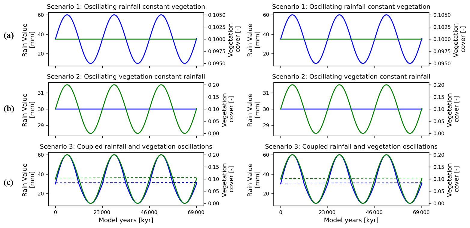
Figure 4Graphical representation of the different precipitation and vegetation forcings applied to the model scenarios described in the text. Forcings for sparse vegetation (10 %) cover are shown on the left and dense vegetation (70 %) cover on the right. Scenarios explored include (a) oscillating precipitation and constant vegetation cover, (b) oscillating vegetation and constant precipitation, and (c) coupled oscillations in precipitation and vegetation cover.
2.2 Boundary and initial conditions
An initial low-relief (<1 m) random-noise topography was applied to the model grid at the start of the simulations. The initial topographies had a slight initial topographic slope of (Fig. 2a). The boundaries on all sides of the domain were closed (no flow) except the southwest corner node, which was an outlet node. From these conditions, the steady-state topography was calculated over 15 Myr model time, and the resulting bedrock elevation and sediment thickness were used as input for the transient scenarios described in Sect. 2.1.
In the following sections, we focus our analysis on the mean catchment sediment thickness (i.e., the combined thickness of soil and regolith) over the entire domain, mean bedrock erosion rates (excluding sediment erosion), mean sediment entrainment rates, and mean catchment erosion rates. The mean catchment erosion rates are the sum of bedrock erosion and sediment entrainment rates. To simplify the presentation, results are shown only for the first cycle of transient climate and vegetation change. Results from the first cycle were representative of subsequent cycles (not shown), and no longer-term variations or trends in erosion–sedimentation were identified or warrant discussion.
3.1 Influence of oscillating precipitation and constant vegetation cover on erosion and sedimentation (scenario 1)
In this scenario, with a rock uplift rate of 0.05 mm a−1 and 23 kyr periodicity in precipitation, the mean catchment sediment entrainment rates follow the pattern of change in precipitation (Fig. 5a and b), but with an offset (phase lag) between the maxima and minima of entrainment and precipitation. A higher variation in the range of sediment entrainment rates (i.e., −0.036 to 0.043 mm yr−1; Fig. 5b) is observed for simulations with 10 % vegetation cover. Negative values in sediment entrainment rates correspond to sediment deposition rates during drier periods. The peak in sediment entrainment rates (e.g., 0.043 mm yr−1 for 10 % veg., and ∼0.038 mm yr−1 for 70 % veg.; Fig. 5b) is observed with a time lag of kyr before the peak in maximum precipitation in both the 10 % and 70 % vegetation cover simulations. This result suggests that as precipitation increases sediment is readily entrained where available in the catchment until bedrock is locally exposed. The changes in mean catchment sediment thickness (Fig. 5c) are influenced by changes in the sediment entrainment and precipitation rates, but with a lag time between the maximum in precipitation and the minimum in sediment thickness. The lowest mean catchment sediment thickness (e.g., ∼0.97 m for 10 % veg., and ∼1.9 m for 70 % veg.; Fig. 5c) also occurs with a time lag of (∼3 kyr) after the peak in precipitation rates for both the 10 % and 70 % vegetation cover simulations. The same time lag ∼3 kyr is observed in the peak in mean catchment bedrock erosion (e.g., ∼0.087 mm yr−1 for 10 % veg. and ∼0.1 mm yr−1 for 70 % veg.; Fig. 5d) and coincides with when the minimum sediment cover is present and more bedrock is exposed for erosion. As we use the total change in bedrock elevation to estimate bedrock erosion rates, the loss in bedrock due to weathering (exponential) is also accounted for. The phase lag in bedrock erosion and sediment thickness can be attributed to exponential weathering, which is discussed in detail in Sect. 4.2. Finally, the mean catchment erosion rates follow the pattern of change in precipitation rates (Fig. 5a and e) without a phase lag. The maximum erosion rates are similar in range for both the 10 % and 70 % vegetation cover simulations (e.g., ∼0.12 mm yr−1; Fig. 5e). However, in the 10 % vegetation cover simulation, the minimum in the mean catchment erosion rate decreases more (e.g., to ∼0.01 mm yr−1; Fig. 5e) relative to the higher-vegetation-cover scenario. The different decreases in the minimum erosion rate between the two vegetation cover amounts correspond to the differences in precipitation rates (Figs. 4a and 5a).
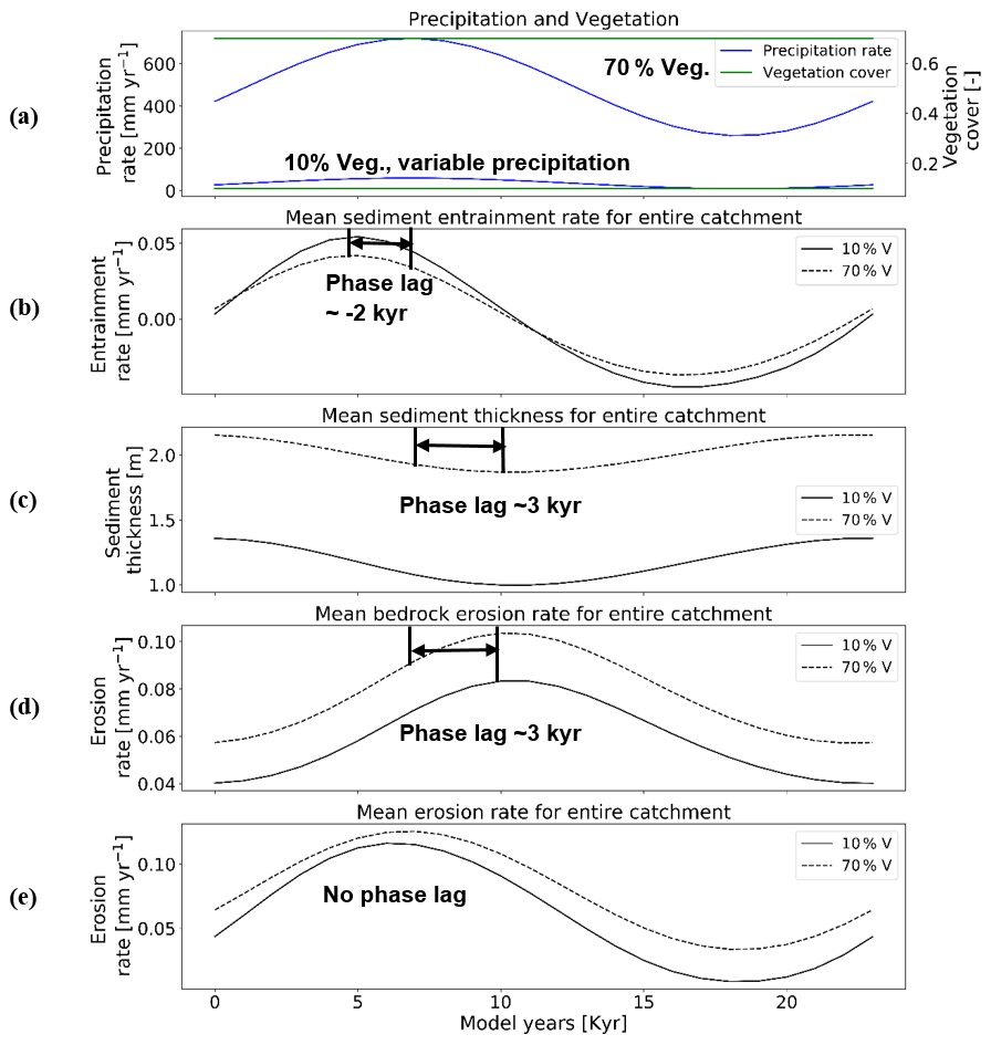
Figure 5Temporal evolution of catchment-averaged predictions for scenario 1 described in the text (Sect. 3.1). Graphical representation of mean catchment sedimentation and erosion to (a) oscillating precipitation [mm yr−1] and constant vegetation cover [–] in terms of (b) sediment entrainment [mm yr−1], (c) sediment thickness [m], (d) bedrock erosion [mm yr−1], and (e) mean erosion rates [mm yr−1] for the entire catchment. The periodicity of climate and vegetation oscillations is 23 kyr with a rock uplift rate of 0.5 mm yr−1.
The absence of a phase lag between the mean catchment erosion and precipitation rates reflects the fact that the combined sediment entrainment and bedrock erosion rates when added together track the overall trend in precipitation rate changes, but the individual components (sediment vs. bedrock) respond differently.
3.2 Influence of constant precipitation and oscillating vegetation cover on erosion and sedimentation (scenario 2)
Results from this scenario with constant mean annual precipitation (at the mean value of the previous scenario) and oscillating vegetation cover (Figs. 4b and 6a) show a starkly different catchment response from scenario 1 (Sect. 3.1). The sediment entrainment rates for both simulations (Fig. 6b) show a small decrease in entrainment as vegetation cover increases (e.g., mm yr−1 for 10 % veg., and mm yr−1 for 70 % veg.; Fig. 6b. As vegetation cover decreases later in the cycle, entrainment rates increase (e.g., to ∼0.13 mm yr−1 for 10 % veg., and to 0.01 mm yr−1 for 70 % veg.; Fig. 6b). The larger magnitude of increase in entrainment for the 10 % vegetation cover case corresponds to the minimum (0 %) vegetation cover for which the potential for erosion is the highest. In the 10 % vegetation cover simulation, the lowest mean catchment sediment thickness was observed ∼1.5 kyr after the minimum in vegetation cover (Fig. 6c).

Figure 6Temporal evolution of catchment-averaged predictions for scenario 2 described in the text (Sect. 3.2). Graphical representation of mean catchment sedimentation and erosion to (a) constant precipitation [mm yr−1] and oscillating vegetation cover [–] in terms of (b) sediment entrainment [mm yr−1], (c) sediment thickness [m], (d) bedrock erosion [mm yr−1], and (e) mean erosion rates [mm yr−1] for the entire catchment. The periodicity of climate and vegetation oscillations is 23 kyr with a rock uplift rate of 0.5 mm yr−1.
The range of mean catchment sediment thickness varies significantly in the simulations (e.g., ∼0.72–1.38 m for 10 % veg., and ∼2.2–∼2.3 m for 70 % veg.; Fig. 6c). The same time lag (∼1.5 kyr) is observed between the peak in mean catchment bedrock erosion rates (Fig. 6d) and the minimum in vegetation cover. This is most likely due to the maximum exposure of bedrock for erosion when catchment average sediment thicknesses are at their minimum. Also, the first phase of the cycle is mainly depositional while bedrock erosion (including weathering) is observed, which happens partly in places where there is no deposition. Finally, mean catchment erosion rates (Fig. 6e) are significantly affected ( mm yr−1) by oscillating vegetation cover in simulations with a mean 10 % vegetation. For the 70 % vegetation cover simulation, a similar maximum in erosion also occurs during the minimum in vegetation but is far less dramatic, presumably due to the still somewhat large (60 %) amount of vegetation cover present. Although the relief and slopes are lower in sparsely vegetated catchment (10 % V), significantly higher erosion rates are observed as precipitation is kept constant at 30 mm yr−1, while the vegetation cover was reduced to 0 %. This can be attributed to low (bedrock–sediment) stream power thresholds.
3.3 Influence of coupled oscillations of precipitation and vegetation cover on erosion and sedimentation (scenario 3)
The catchment response to coupled oscillations in precipitation rate and vegetation cover (Fig. 4c) for erosion and sedimentation represents a composite of the effects discussed in the previous two sections (Fig. 7). For example, the mean catchment sediment entrainment rates have a peak in entrainment rates (∼1.5 kyr) prior to the peak in climate–vegetation values. A similar effect was noted for scenario 1 (Fig. 5, Sect. 3.1). As the precipitation rates and vegetation cover decrease later in the cycle (Fig. 7a), the sediment entrainment rates increase. In more detail, the 70 % vegetation cover simulations show a modest increase similar to that observed in scenario 1 (Fig. 5b), whereas the 10 % vegetation cover shows a sharp peak in the sediment entrainment rates when 0 % vegetation cover is present. This latter observation is similar to what is observed for scenario 2 (Fig. 6b, Sect. 3.2). Thus, in the case of covarying precipitation rates and vegetation cover, the response observed in terms of sediment entrainment is not predicted to be the same for all degrees of vegetation cover and depends heavily on the initial vegetation cover of the system around which variations occur.
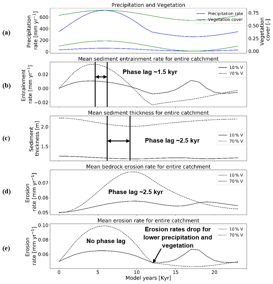
Figure 7Temporal evolution of catchment-averaged predictions for scenario 3 described in the text (Sect. 3.3). Graphical representation of mean catchment sedimentation and erosion to (a) coupled oscillations in precipitation [mm yr−1] and vegetation cover [–] in terms of (b) sediment entrainment [mm yr−1], (c) sediment thickness [m], (d) bedrock erosion [mm yr−1], and (e) mean erosion rates [mm yr−1] for the entire catchment. The periodicity of climate and vegetation oscillations is 23 kyr with a rock uplift rate of 0.5 mm yr−1.
Mean catchment sediment thicknesses in the 10 % vegetation cover simulation show a modest response and vary between 1.16 and 1.24 m (Fig. 7c), with a time lag of ∼2.5 kyr between the peak in precipitation–vegetation and minimum sediment thickness. This lag is also observed in the case of the 70 % vegetation cover simulation, but with a higher amplitude of change in sediment thickness (e.g., 2–2.22 m; Fig. 7c). A similar trend in time lags between the peaks in climate–vegetation and bedrock erosion (Fig. 6d) is also present. These observations for variations in sediment thickness again represent the combined effects of the results discussed in Sect. 3.1 and 3.2 (Figs. 5c and 6c).
The amplitude of change in bedrock erosion is 0.05–0.06 mm yr−1 for 10 % veg. and 0.05–0.08 mm yr−1 for 70 % veg. (Fig. 7d). The bedrock erosion response for both simulations represents a composite of the effects shown in the previous two scenarios (Sect. 3.1 and 3.2). Here the increase in time lag in the maximum in erosion rates (most notable for the 70 % vegetation cover simulation) resembles the effect of a large increase in precipitation rates (compared to Fig. 5d) for the first part of the cycle. Whereas the second peak in bedrock erosion visible in the 10 % vegetation cover scenario more closely resembles the effects shown in Fig. 6d when the vegetation cover goes to 0 %, the landscape is increasingly sensitive to erosion with whatever runoff (albeit little) is available.
Finally, the mean catchment erosion rates (Fig. 7e) again show the combined effects of the sediment entrainment rate and bedrock erosion histories previously discussed (Fig. 7b and d). In the simulation with 70 % initial vegetation cover, the mean catchment erosion rates follow the pattern of changes in precipitation rates (e.g., ranging from 0.04 to 0.1 mm yr−1; Fig. 7e, see also Fig. 5e). A similar trend is present in the first half of the cycle in the simulation with 10 % vegetation cover, but with much lower magnitudes (i.e., 0.05 to 0.06 mm yr−1; Fig. 7e). However, during the second half of the cycle, the erosion rates increase up to ∼0.06 mm yr−1 and have a second peak at ∼17–18 kyr for the 10 % vegetation simulation when the vegetation cover is at 0 %. The previous result is, however, in contradiction to the detachment-limited results shown in Fig. 17 of Schmid et al. (2018), who found that erosion rates decreased to 0 mm yr−1 for the period of no vegetation cover and a minimum precipitation rate of ∼10 mm yr−1. This contradiction is related to the increase in sediment entrainment at this time (Fig. 7b), which heavily influences the mean erosion. The detachment-limited approach of Schmid et al. (2018) could not account for this and will be discussed in detail in Sect. 4.2. To summarize, as discussed previously the locations of the maximums and minimums in the mean erosion rate and the shape of the curves (Fig. 7e) can be linked to different times in the climate and vegetation history when either the effects of variable precipitation rate or vegetation cover dominate the mean catchment erosional response.
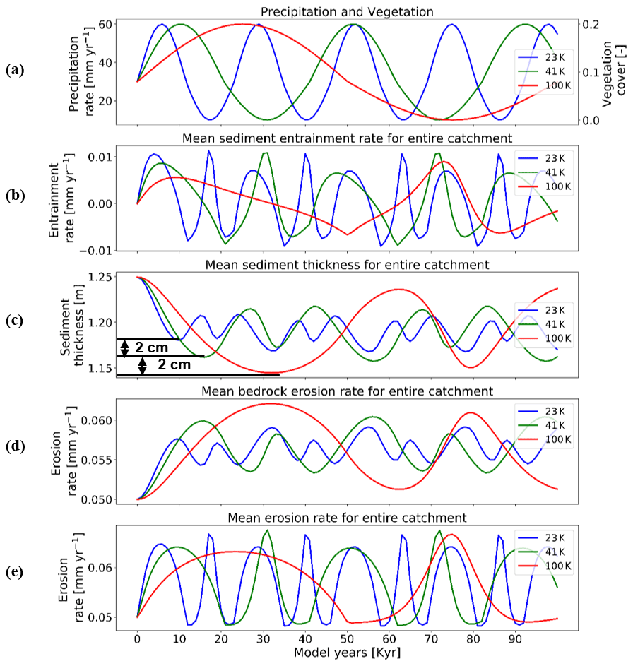
Figure 8Temporal evolution of catchment-averaged predictions for scenario 4 described in the text (Sect. 3.4). Graphical representation of mean catchment sedimentation and erosion to (a) different periodicities of coupled oscillations in precipitation [mm yr−1] and vegetation cover [–] in terms of (b) sediment entrainment [mm yr−1], (c) sediment thickness [m], (d) bedrock erosion [mm yr−1], and (e) mean erosion rates [mm yr−1] for the entire catchment. The rate of rock uplift is kept constant at 0.5 mm yr−1. The simulations represent 10 % initial vegetation cover.
3.4 Influence of the periodicity of precipitation–vegetation variations on erosion and sedimentation (scenario 4)
Here we show the influence of different periodicities (23, 41, and 100 kyr) in precipitation and vegetation change on catchment erosion and sedimentation for the cases of a 10 % mean vegetation cover (Fig. 8) and 70 % vegetation cover (Fig. 9). We find higher variations in mean sediment entrainment rates (Figs. 8b and 9b) for both the 10 % and 70 % vegetation cover simulations for the shorter periodicities (23 and 41 kyr). However, the phase lag in the peaks of sediment entrainment and precipitation rates was higher for longer periodicities (e.g., ∼9 %, ∼16.2 %, ∼19 % in 23, 43, and 100 kyr, respectively) for the 10 % vegetation cover case (Fig. 8b). These phase lags are, however, dampened in the highly vegetated landscapes (70 %) at longer periods (i.e., ∼9 %, ∼9.5 %, ∼14 % in 23, 43, and 100 kyr, respectively; Fig. 9b). In a landscape with 10 % vegetation cover, the simulation with longer periodicity (100 kyr) shows higher variations in mean catchment sediment thickness (e.g., 1.14–1.25 cm; Fig. 8c). This is mimicked in the landscape with 70 % vegetation cover, with the range of sediment thickness between 1.95 and 2.27 cm (Fig. 9c). A similar trend with a higher amplitude of change is also observed for bedrock erosion rates in the sparsely vegetated landscape (10 %) with values ranging from 0.05 to 0.062 mm yr−1 (Fig. 8d) for longer periodicity (100 kyr). The same pattern is observed in highly vegetated landscapes (70 %), with the values of bedrock erosion rates ranging from 0.045 to 0.094 mm yr−1 (Fig. 9d) for the longer periodicity (100 kyr).

Figure 9Temporal evolution of catchment-averaged predictions for scenario 4 described in the text (Sect. 3.4). Graphical representation of mean catchment sedimentation and erosion to (a) different periodicities of coupled oscillations in precipitation [mm yr−1] and vegetation cover [–] in terms of (b) sediment entrainment [mm yr−1], (c) sediment thickness [m], (d) bedrock erosion [mm yr−1], and (e) mean erosion rates [mm yr−1] for the entire catchment. The rate of rock uplift is kept constant at 0.5 mm yr−1. The simulations represent 70 % initial vegetation cover.
Overall variations in mean catchment erosion rates (Figs. 8e and 9e) were not observed to be significant (<0.0001 mm yr−1) as the period of precipitation and vegetation change increases.
3.5 Influence of rock uplift rate and oscillating precipitation–vegetation on erosion sedimentation (scenario 5)
Here we investigate the response of mean catchment erosion and sedimentation for different rates of rock uplift (i.e., 0.05, 0.1, 0.2 mm yr−1) for the 10 % vegetation cover (Fig. 10) and 70 % vegetation cover (Fig. 11) scenarios. To simplify the presentation and comparison of results, the periodicity of precipitation and vegetation change is kept the same as in Sect. 3.3 (i.e., 23 kyr). In general, the results discussed below demonstrate the fact that the transient catchment response to coupled oscillations in precipitation rate and vegetation cover are similar in shape regardless of the rock uplift rate. The magnitude of change in mean catchment erosion associated with precipitation and vegetation changes increases with increasing uplift rate, despite an identical amount of vegetation and precipitation change imposed (Figs. 10a and 11a) on each rock uplift rate simulation.
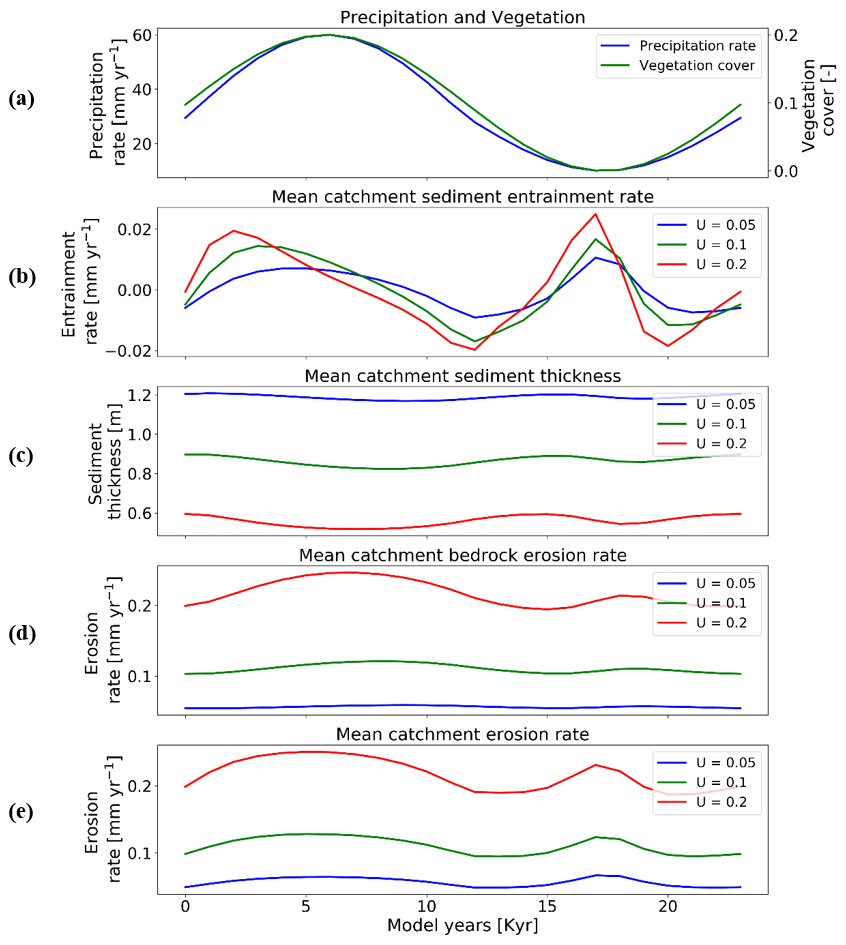
Figure 10Temporal evolution of catchment-averaged predictions for scenario 5 described in the text (Sect. 3.5). Graphical representation of mean catchment sedimentation and erosion with different rates of rock uplift [mm a−1] to (a) coupled oscillations in precipitation [mm yr−1] and vegetation cover [–] in terms of (b) sediment entrainment [mm yr−1], (c) sediment thickness [m], (d) bedrock erosion [mm yr−1], and (e) mean erosion rates [mm yr−1] for the entire catchment. The periodicity of climate and vegetation oscillations is 23 kyr. The simulations represent 10 % initial vegetation cover.

Figure 11Temporal evolution of catchment-averaged predictions for scenario 5 described in the text (Sect. 3.5). Graphical representation of mean catchment sedimentation and erosion with different rates of rock uplift [mm a−1] to (a) coupled oscillations in precipitation [mm yr−1] and vegetation cover [–] in terms of (b) sediment entrainment [mm yr−1], (c) sediment thickness [m], (d) bedrock erosion [mm yr−1], (e) mean erosion rates [mm yr−1] for entire catchment. The periodicity of climate and vegetation oscillations is 23 kyr. The simulations represent 70 % initial vegetation cover.
In more detail, the temporal pattern of changes in sediment entrainment rates (Figs. 10b and 11b) is similar for all uplift rates considered, but the amplitude of change increases as the uplift rate increases. In addition, the phase lag between the peaks in sediment entrainment rates and maximum precipitation rates in the 10 % vegetation simulation (Fig. 10b) varies with the rock uplift rate. For example, the peaks in sediment entrainment rates have a phase lag of kyr, −2.5, and −2 kyr for rock uplift rates of 0.2, 0.1, and 0.05 mm a−1, respectively (Fig. 10b), in first half of the vegetation–precipitation oscillation. However, the phase lags are overall shorter in highly vegetated landscapes (70 %) (e.g., , −2, −1 kyr) before the maximum in precipitation for rock uplift rates of 0.2, 0.1, and 0.05 mm a−1, respectively (Fig. 11b).
For the landscape with 10 % vegetation cover, the simulation with the highest rates of rock uplift (0.02 mm a−1) showed lower mean catchment sediment thickness (e.g., ∼0.5–∼0.6 m; Fig. 10c). In contrast, the slowest rock uplift simulation (0.05 mm a−1) had thicker sediment of ∼1.16–∼1.24 m (Fig. 10c). The same pattern was observed in the catchment with 70 % vegetation cover: the higher sediment thicknesses occur for the lower rates of rock uplift (e.g., ∼2–∼2.2 m; Fig. 11c). These results for sediment thickness variations reflect the fact that higher rock uplift rates result in steeper slopes (not shown) and higher mean catchment erosion rates (Figs. 10e and 11e) such that regolith production rates are outpaced by erosion and therefore result in thinner sediment. Also, the thicker sediment for lower uplift rates could be an integrated result of slightly lower erosion rates compared to sediment production rates over the whole 15 Myr model runtime (steady state). This result is akin to the observational results from Heimsath et al. (1997).
Temporal variations in bedrock and mean catchment erosion rates are similar to those described in Sect. 3.3 (Fig. 7) for the sparsely and more heavily vegetated conditions. The primary difference is that at high rock uplift rates the amplitude of bedrock or mean catchment erosion increases (Figs. 10d, e and 11d, e). To summarize, these results highlight the fact that regardless of the rock uplift rate, similar temporal changes are observed in sediment entrainment or thickness and in bedrock and catchment erosion for oscillating precipitation rates and vegetation cover. However, the amplitude of change (or absolute change) in entrainment and erosion rates increases with increases in rock uplift rate. This will be discussed in detail in Sect. 4.4.
In this section, we synthesize the results from previous sections (scenarios 1–5) in detail. We further investigate the effects of coupled climate and vegetation oscillations (scenario 3) on the occurrence of erosion and sedimentation on a spatial scale.
4.1 Differences in effects between oscillating vegetation or precipitation
Here the sensitivity of erosion and sedimentation to variable precipitation and/or vegetation cover is analyzed. In the scenario with oscillating precipitation and constant vegetation cover, sparsely vegetated landscapes (10 %) erode slowly during periods of lower precipitation. This might be attributed to the dependency of the bedrock erosion and sediment entrainment on the amount of water available through precipitation, which in turn affects the erosion rates. The mean erosion in this scenario is dominated by bedrock erosion with a significant contribution from sediment entrainment. Also, the mean erosion rates over one climate oscillation cycle are observed to be slightly higher (∼20 %) than mean erosion rates at steady state for sparsely vegetated landscape (10 % V). For densely vegetated landscape (70 % V), this difference is significant (i.e., 50 % higher mean erosion rates during a transient cycle in comparison to steady state). This implies the nonlinearity of the erosion response to changes in MAP, which is significantly higher in a densely vegetated landscape where the amplitude of change in MAP (e.g., 260–720 mm) is much higher than drier landscapes (e.g., 10–60 mm).
Similarly, in a scenario with constant precipitation and variable vegetation cover, sparsely vegetated landscapes (10 %) are observed to be much more sensitive in terms of erosion rates during periods of no vegetation cover. The amplitude of erosional change was 10 times higher than that of densely vegetated landscapes. The mean erosion in sparsely vegetated landscapes is dominated equally by bedrock erosion (Fig. 6d) and sediment entrainment due to the higher availability of bare soil. This justifies the argument of a higher sensitivity of sparsely vegetated landscapes to erosion and sedimentation. This result confirms the findings of Yetemen et al. (2015) (see Fig. 2g), which suggests that shear stress (erosion) decreases significantly (1 to 0.1) as the total grass cover (vegetation) is increased from 0 % (bare soil) to 20 %. Also, a small change in vegetation cover in densely vegetated landscapes would not result in significant differences in erosional processes. Unlike the previous scenario (oscillating precipitation and constant vegetation cover), we do not observe nonlinearity in erosion response to the changes in vegetation cover (i.e., mean erosion rates over one transient cycle are equal to steady-state mean erosion rates).
In general, mean catchment sediment thickness is observed to be inversely proportional to precipitation owing to higher stream power. This in turn translates to a higher sediment flux during wetter periods. The influence of oscillating precipitation and constant vegetation cover on sediment thickness is slightly higher in simulations with sparse vegetation cover. In simulations with constant precipitation and oscillating vegetation cover, the sensitivity of sediment thickness is much higher in landscapes with sparse vegetation. This can be attributed to an absence of vegetation cover. A decreased impact of oscillating vegetation cover on sediment thickness occurs in landscapes with denser vegetation cover and demonstrates that surface processes in these settings are not highly dependent on changes in vegetation density. This has been explained by Huxman et al. (2004), who found that vegetation cover responds to MAP variations in wet and dry systems during dry years.
4.2 Synthesis of coupled oscillations of precipitation and vegetation cover simulations
The sensitivity of erosion and sedimentation to coupled oscillations in precipitation and vegetation cover (scenario 3, Sect. 3.3) indicates that mean catchment erosion rates (Fig. 7e) are correlated with precipitation for densely vegetated landscapes (70 %). This is due to the dominating effect of mean annual precipitation changes (from 26 to 72 cm yr−1) on erosion over vegetation cover change (from 60 % to 80 %; Fig. 7a) in these landscapes. This can be attributed to the higher amplitude of precipitation oscillations in these simulations required to change vegetation cover by ±10 % (Fig. 2b). In the case of a sparsely vegetated landscape (10 %), mean erosion rates (Fig. 7e) are also correlated with precipitation, but only for the first half of the cycle when vegetation cover is present. However, mean erosion rates increase rapidly in the second half of the cycle when MAP decreases (from 60 to 10 mm yr−1; Fig. 7a) and vegetation cover magnitudes decrease (from 20 % to 0 %; Fig. 7a). This inverse correlation between precipitation and erosion can be attributed to increasing susceptibility of the surface to sediment entrainment as vegetation cover decreases to bare soil, even with very low precipitation rates. The nonlinearity of erosion response to changes in MAP is reduced by half (in comparison to changing climate and constant vegetation) in coupled simulations.
Thus, the temporal evolution of mean erosion rates between heavily (70 %) and sparsely (10 %) vegetated landscapes varies depending on the initial vegetation state of the catchment. As a result, correlated and anticorrelated relationships between precipitation, vegetation cover, and erosion are predicted and are the result of precipitation or vegetation exerting a dominant or subsidiary influence on catchment erosion at different times in the catchment history and for different catchment precipitation and vegetation cover conditions. This prediction is consistent with observed correlations of vegetation cover and catchment average erosion rates recently documented along the western Andean margin by Starke et al. (2020).
The lag behavior observed in sediment entrainment, thickness, and bedrock erosion is explained in additional simulations we conducted (results not shown for brevity) wherein the weathering (regolith production) function was turned off in the model simulations (see Fig. A1). In these simulations, we did not observe any significant phase lags in maximum and minimum erosion rates, sediment thickness, or vegetation cover–precipitation. Also, the erosion rates for sparsely vegetated catchment (10 % V) drop to a minimum during the phase of bare soil and minimum precipitation (10 mm yr−1). Hence, sediment supply through weathering can be attributed to double peaks observed in mean catchment sediment entrainment rates (Fig. 7b) and erosion rates (Fig. 7e). When there is no explicit weathering–regolith production involved in the model simulations, sediment supply for entrainment is significantly reduced. As a result, entrainment rates are observed to be 2 orders of magnitude lower than bedrock erosion; hence, entrainment rates are not shown in Fig. A1. This implies that weathering plays a major role in leading to the phase lags observed in the above results.
4.3 Differences between the periodicities of climate and vegetation cover oscillations
The periodicity of change in climate will mainly affect vegetation via the lag time it takes for the vegetation to respond; i.e., if the vegetation structure does not change (e.g., grasslands or forests), then grasslands are very flexible (Bellard et al., 2012; Kelly and Goulden, 2008; Smith et al., 2017). Grasslands can plastically respond from year to year, while forests may die off and be replaced by grasslands when it becomes drier and vice versa. This change in vegetation type might lead to the fluctuations in sedimentation and erosion rates due to periodicity of change in climate and vegetation cover.
4.4 The effect of rock uplift rate on signals of varying precipitation and vegetation cover
No difference in erosion rates was identified between the two different vegetation–precipitation simulations for a given uplift rate when the erosion rate is averaged over the full period of vegetation–precipitation change. In a steady-state landscape, erosion rates are equal to the rock uplift rates according to the law of continuity of mass (e.g., Tucker et al., 2001). This means that steady-state landscapes experience higher erosion rates with higher uplift rates. However, the mean catchment erosion rates shown in Figs. 10e and 11e show temporal variations in the erosion rate driven by oscillations in the precipitation rate and vegetation. When average erosion rates are calculated over a complete cycle of the oscillation, the mean erosion rates are slightly higher than rock uplift rates owing to the nonlinearity of erosion response to changes in MAP. This result indicates that any climate- or vegetation-driven changes in erosion will not be evident when observed over too long a period of time, but they might introduce shorter-term transients (high or low) depending on the climate–vegetation cycle of change. This finding is significant for observational studies seeking to measure the predictions shown in this study. More specifically, thermochronometer dating approaches used to quantify denudation rates over million-year timescales will be hard-pressed to measure any signal of how climate or vegetation change on Milankovitch timescales influences denudation. Rather, the rate of tectonic rock uplift or exhumation (in the case of erosion rates equalling the rock uplift rate) will be measured. In contrast, observational techniques sensitive to decadal (e.g., sediment fluxes) or millennial (e.g., cosmogenic radionuclides measured from river terraces) processes can be sensitive to timescales less than the period of oscillation and are more likely to record transient catchment erosion rates influenced by variations in precipitation or vegetation cover.
The vegetation- and precipitation-driven transients in mean catchment erosion rates predicted by this study were large enough to be measured by some observational techniques. For example, in sparsely vegetated landscapes the half-amplitude of change in erosion rates (from steady-state values) slightly decreases as the uplift rate increases. A higher magnitude of change in transient erosion rates (from steady-state values) is found in densely vegetated landscapes and is again slightly decreased as the uplift rate increases. Previous work by Schaller and Ehlers (2006) investigated the ability of denudation rates calculated from cosmogenic radionuclides measured in a sequence of fluvial terraces to record periodic (Milankovitch timescale) variations in denudation rates. The magnitude of change in predicted transient erosion rates described above is above the detection limit reported by Schaller and Ehlers (2006), particularly when the mean catchment denudation rate is ∼0.1 mm yr−1 or higher. Thus, the predictions suggested in this study are testable in field-based studies, and other methods such as basin sedimentation rate histories (e.g., determined from magneto-stratigraphy, optically stimulated luminescence, or other methods) also hold potential.
4.5 Spatial changes in where erosion and sedimentation changes occur
In the previous sections, our analysis focused on the spatially averaged response of the catchment in terms of changes in sedimentation and erosion. Here, we discuss the same model results as previously presented for but show two examples (for two different vegetation covers) of the spatial variations of erosion and sediment thickness within the catchments. This provides a basis for understanding where in the catchment changes are occurring.
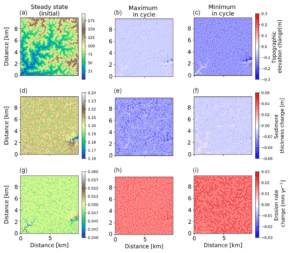
Figure 12Two-dimensional map-view representation of changes in topographic elevations [m] (a–c), sediment thickness [m] (d–f), and erosion rates [mm yr−1] (g–i). These changes are represented with respect to steady-state conditions (a, d, g) for maximum (b, e, h) and minimum (c, f, i) values of precipitation and vegetation in an oscillation cycle. The simulations represent 10 % initial vegetation cover.
Spatial variations in the pattern of erosion and sedimentation in the simulations with 23 kyr coupled precipitation and vegetation oscillations, as well as a rock uplift rate of 0.05 mm a−1, are shown in the topographic elevation, sediment thickness, and erosion rate changes for both the maximum and minimum in precipitation and vegetation cover. In the simulations with sparse vegetation cover (10 %) (Fig. 12) at the maximum in precipitation and vegetation cover, erosion rate changes from steady state are ∼0.03 mm yr−1 in valleys and ∼0.01 mm yr−1 on hillslopes. At the minimum in precipitation and vegetation cover, erosion rate changes from steady state are higher in valleys than hillslopes. This may be attributed to an absence of vegetation during this period, when the surface (bedrock or sediment) is readily available for erosion even with lower precipitation rates. The sediment thickness is observed to be slightly higher in the streambeds and valleys for streams with larger accumulation area. However, the smaller streams have lower sediment thickness compared to connected hillslopes. For example, higher sediment thickness (∼1.24 m) is observed near the catchment outlet in the lower left corner of the domain. At the maximum in the precipitation and vegetation cover cycle, the landscape experiences a slightly higher contrast in sediment thickness compared to the steady-state condition, whereby a net lowering of the sediment layer is observed of approximately 2 to 5 cm on the hillslopes and ∼6 cm near the catchment outlet. This can be attributed to higher sediment fluxes during this period. At the minimum in the precipitation and vegetation cover cycle, the landscape experiences a slight difference from the steady-state sediment thickness (∼2 cm lowering) except for deposition in higher-order streams (up to ∼2 cm) near the catchment outlet.
In the simulations with dense vegetation cover (70 %) (Fig. 13), erosion rate changes from steady-state conditions are higher during the maximum in the precipitation and vegetation cover cycle with higher magnitudes (∼0.08 mm yr−1 in valleys and up to ∼0.02 mm yr−1 on hillslopes and ridges) due to the higher precipitation rates. At minimum precipitation and vegetation cover magnitudes (P=26 cm; V=60 %), erosion rate changes are reduced (up to −0.03 mm yr−1) in valleys and (up to −0.01 mm yr−1) on hillslopes in comparison to the erosion rates at steady state. Sediment thickness is observed to be relatively higher in the streambeds and valleys (∼2.25 m) than the hillslopes. It is contrastingly higher in the lowlands than the areas at higher elevations. At maximum precipitation and vegetation cover (maximum in the cycle) sediment thickness is ∼10 cm lower on hillslopes and up to ∼30 cm lower in valleys. The same trend with lower amplitude is evident for the minimum in the precipitation and vegetation cover cycle. This implies that at higher vegetation cover, sediment thickness is significantly reduced as a result of higher sediment flux during the peak in precipitation rates. This in turn signifies the dominance of precipitation changes over vegetation cover change in highly vegetated landscapes.
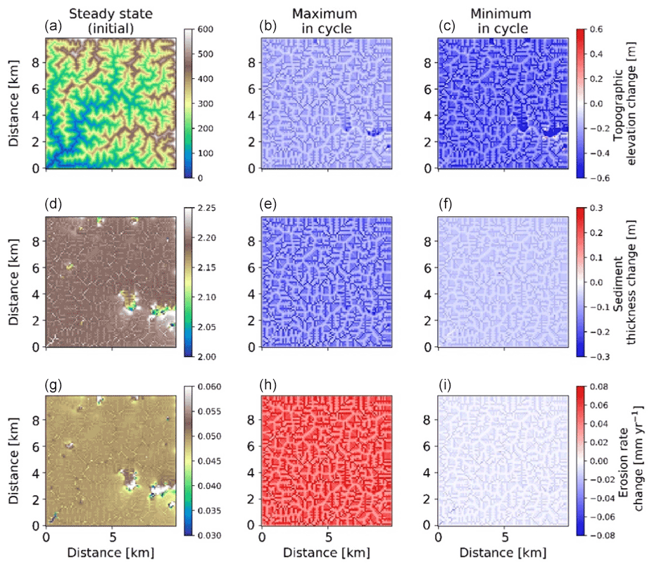
Figure 13Two-dimensional map-view representation of changes in topographic elevations [m] (a–c), sediment thickness [m] (d–f), and erosion rates [mm yr−1] (g–i). These changes are represented with respect to steady-state conditions (a, d, g) for maximum (b, e, h) and minimum (c, f, i) values of precipitation and vegetation in an oscillation cycle. The simulations represent 70 % initial vegetation cover.
4.6 Comparison to previous studies
Results presented in this study document a higher sensitivity of catchment erosion and sedimentation of sparsely vegetation landscapes (10 %) to changes in vegetation cover, whereas densely vegetated (70%) landscapes are more responsive to changes in precipitation than vegetation changes. This confirms the broad findings of Schmid et al. (2018) and Yetemen et al. (2019), which suggest vulnerability of erosion rates in sparsely vegetated landscapes to changes in vegetation cover and, for densely vegetated landscapes, sensitivity to the changes in MAP. However, there are differences between the results of Schmid et al. (2018) and this study, particularly for the temporal changes in erosion rates we observe for the sparse-vegetation-cover (10 %) scenario with coupled precipitation–vegetation cover oscillations. More specifically, previous results from the detachment-limited model shown in Fig. 17 of Schmid et al. (2018) show that catchment erosion rates in sparsely vegetated landscapes decrease as the precipitation and vegetation cover increases in the first part of a cycle. In the second part of the cycle when precipitation and vegetation decrease to their minimum Schmid et al. (2018) predict erosion rates of ∼0 mm yr−1. However, in the coupled detachment–transport fluvial erosion model presented here (SPACE), we observe a different behavior and erosion rates slightly increase as precipitation and vegetation cover increase (from 0.05 to 0.065 mm yr−1; Fig. 7e), rather than decrease. This difference is due to the higher sediment entrainment rates we predict during the period of no vegetation and low precipitation (10 mm yr−1), which is a result of higher vulnerability of bare soil to erosion, even with very low precipitation rates. Therefore, the application of a detachment-limited vs. coupled detachment–transport-limited modeling approach has bearing on the predicted response, and when comparing results to natural systems care should be taken in which approach is used.
Previous geochemistry-related observational studies from the Chilean Coastal Cordillera (EarthShape study areas, https://esdynamics.geo.uni-tuebingen.de/earthshape/index.php?id=129, last access: 15 January 2021) are also available for comparison to this study. For example, the steady-state sediment thicknesses in our simulations for 10 % and 70 % initial vegetation cover are predicted to be higher than the field observations reported by Schaller et al. (2018) and Oeser et al. (2018), who reported a ∼20 and ∼60 cm depth of mobile sediment layers on hillslopes in the Pan de Azucar and La Campana study areas, respectively. Also, the natural topography is steeper with higher relief, and rock uplift rates might be different. Spatial variations in vegetation also occur (e.g., in La Campana), with higher vegetation density along valleys, which might lead to the discrepancies between the observed and predicted sediment thickness. However, the trend in our results (higher sediment thickness for densely vegetated – 70 % – landscapes) follows the findings of Oeser et al. (2018), who document sediment increase with increasing mean annual precipitation and vegetation in the Chilean Coastal Cordillera.
In addition, previous field studies (Oeser et al., 2018; Owen et al., 2011; Schaller et al., 2018) applied cosmogenic nuclides to estimate the denudation and soil production rates in the Chilean Coastal Cordillera. They suggest an increase in soil production rates from arid zones in the north to wet tropical zones in the south of the Chilean Coastal Cordillera. These findings are consistent with the predicted increase in sediment depths (e.g., 1.24 m for V=10 % and 2.22 m for V=70 %; Fig. 7b) in our study. Finally, the effects of rock uplift and precipitation rates on topography and erosion rates, as documented by Bonnet and Crave (2003) and Lague et al. (2003), show a linear relationship between mean topographic elevation and rock uplift rate for steady-state conditions.
4.7 Model limitations
The model setup used in this study was intended to quantify the sensitivity of hillslope and fluvial erosion as well as sediment transport and depositional processes for different climates with variations in precipitation rates and vegetation cover over Milankovitch timescales. This study was designed as an incremental step forward from previous modeling studies (Collins et al., 2004; Istanbulluoglu and Bras, 2005, 2006; Schmid et al., 2018).
There are several simplifying assumptions made in our modeling approach that warrant discussion and potential investigation in future studies. For example, this study assumed uniform vegetation cover and lithology for the entire catchment. The assumption of uniform vegetation cover in the catchment is likely reasonable given the relatively small (10×10 km2) size of catchments investigated and the modest topographic relief produced (between ∼75–600 m; Fig. 10a). Although temperature and precipitation (and therefore vegetation cover) can vary with elevation, the generally low relief of the catchments in this study does not make this a major concern. Due to the long (geologic) timescales considered in this study and computational considerations, mean annual precipitation rates were applied and stochastic distributions of precipitation could not be considered. While our approach is common for landscape evolution modeling studies conducted on geologic timescales, we recognize that in some settings (such as the arid region of this study; Fig. 1) precipitation events are rare, stochastic in nature, and might have an influence on the results presented here. This is a caveat that warrants future investigation.
The vegetation–erosion parameterization considered in this study follows from that of Istanbulluoglu and Bras (2006) and Schmid et al. (2018). In this parameterization the total vegetation cover of the catchment is considered only, rather than the distribution of vegetation cover by individual plant functional types (e.g., grass, shrubs, trees) that would have different Manning's coefficients associated with them. The “total vegetation cover” approach used in our (and previous) work is a reasonable starting point for understanding landscape evolution over large spatial and temporal scales because (a) more detailed observations about the changes in the distribution of plant functional types over Milankovitch timescales is not available and would be poorly constrained, and (b) empirical relationships between total vegetation cover and precipitation are available and easily implemented (e.g., Fig. 2b). However, future work should focus on exploring how the temporal and spatial distribution of different plant functional types during changing climate impacts catchment erosion given that recent work (Mishra et al., 2019; Starke et al., 2020) has identified this as important. This limitation can be handled in future studies with the full coupling of dynamic vegetation models, such as LPJ-GUESS (Smith et al., 2014; Werner et al., 2018), to a landscape evolution model for the explicit treatment of how different vegetation types change temporally and spatially within a catchment and influence catchment erosion. Also, the total vegetation cover in the model is not disturbed by flow and entrainment, which were observed to have a large impact on the results of Collins et al. (2004) and Istanbulluoglu and Bras (2005). If the vegetation cover was spatiotemporally influenced by the above processes in our simulations, the resulting erosion and sedimentation would have been hybrid between sparse (10 % V) and densely vegetated (70 % V) catchments, with vegetation losses in channels. The timescale for the current study was based on Milankovitch cycles to address the effects of periodicity on erosion and sedimentation. However, the effects of seasonal (sub-annual) variations in precipitation (Istanbulluoglu and Bras, 2006; Yetemen et al., 2015) and satellite-derived vegetation cover (with catchment-variable plant function type distributions) also warrant future investigation to determine if coupled seasonal variations in vegetation cover and precipitation influence catchment erosion.
Finally, the results of this study rely upon the vegetation–erosion parameterizations described in Sect. 2 and the Appendix (see also Fig. 3). While there is an observational basis for these relationships (see Sect. A1 and A2), there are, frankly, a sparse number of field studies available robustly constraining how different vegetation types and amounts influence hillslope and surface water erosional processes. Thus, we consider the erosional parameterizations used here to be hypotheses (rather than robust geomorphic transport laws) that warrant investigation in future field or flume studies.
In this study, we investigate the effects of variable vegetation cover and climate over Milankovitch timescales on catchment-scale erosion and sedimentation. Simulations were presented to document if these transients are muted (lower amplitude) at higher rock uplift rates. The approach used here complements previous studies by using a coupled fluvial detachment–transport-limited and hillslope diffusion landscape evolution model, and it also investigates the degree to which transient effects of vegetation cover and precipitation are measurable in observational studies. The main conclusions deduced from this study are the following.
- i.
The stepwise increase in complexity of the model simulations was essential for identifying temporal changes in catchment erosion and sediment thickness. A nonlinear response in erosion and sediment thickness to varying precipitation and vegetation cover was observed, and results were dependent on the initial vegetation and precipitation state of the catchment. The sources of nonlinearity stem from (a) a nonlinear relationship between precipitation changes required to cause a ±10 % change in vegetation cover (Fig. 2) and (b) exponential and power-law relationships in the prescribed vegetation-dependent hillslope and fluvial, respectively, geomorphic transport laws (Fig. 3, see also the Appendix).
- ii.
Analysis of results for covarying precipitation and vegetation cover indicates that erosion and sedimentation in densely vegetated landscapes (V=70 %) are more heavily influenced by changes in precipitation than changes in vegetation cover. This is due to the higher amplitude of precipitation change needed to cause variations in vegetation cover in densely vegetated settings (Figs. 5a and 7e).
- iii.
Analysis of results for covarying precipitation and vegetation cover indicates that erosion and sedimentation in sparsely vegetated landscapes (V=10 %) are more sensitive to variable vegetation cover with constant precipitation rates (Figs. 6 and 7e), particularly when precipitation rates decrease and vegetation cover approaches 0 %.
- iv.
Concerning the first hypotheses stated in the Introduction, we found that the effect of Milankovitch periodicity variations on the amplitude of change in sediment thickness and bedrock erosion is more pronounced for longer climate and vegetation oscillations (100 kyr) in both climate and vegetation settings. This finding confirms the hypothesis. Furthermore, periodicity effects on erosion and sediment thickness are larger in densely (70 %) vegetated landscapes than sparsely (10 %) vegetated landscapes, thereby indicating a sensitivity of the response to the biogeographic zone the changes are imposed on.
- v.
With respect to our second hypothesis, all transient forcings in precipitation and vegetation cover explored in this study resulted in variations in erosion and sediment thickness around the mean erosion rate, which is determined by the rock uplift rate. As rock uplift rates increased from 0.05 to 0.2 mm a−1, the effects of periodic changes in precipitation and vegetation cover on erosion rates became more pronounced and were between about 35 % and 110 %, respectively, of the background rock uplift rate. This finding negates the hypothesis and suggests that regardless of the tectonic setting considered (within the range of rock uplift rates explored here) erosional transients from varying precipitation and vegetation cover occur, but the detection of these changes requires measurement of erosion rates integrating over short timescales such that the average (tectonically driven) mean erosion rate is not recovered.
- vi.
Finally, in comparison to previous studies, the 35 % to 110 % transient changes in erosion rate documented here are at, or above, the detection limit for measurement cosmogenic radionuclides in river sediments preserved in fluvial terraces, but they would be undetectable with bedrock thermochronometer dating techniques that average erosion rates over longer timescales. The potential to measure vegetation-related transient changes in erosion rates with cosmogenic nuclides is highest in settings with higher rock uplift rates (e.g., 0.1 and 0.2 mm a−1) and at longer (41 to 100 kyr) periodicities.
The approach in our study follows the law of continuity of mass (e.g., Tucker et al., 2001). It states that the rate of change in topographic elevation (z) is defined as follows:
where U is uplift rate [m yr−1] and t is time [yr]. The second and third terms on the right-hand side refer to the rate change in topographic elevation due to fluvial and hillslope processes, respectively.
A1 Vegetation-dependent hillslope processes
The rate of change in topography due to hillslope diffusion (Fernandes and Dietrich, 1997; Martin, 2000) is defined as follows:
where qs is sediment flux along the slope S. We applied the slope- and depth-dependent linear diffusion rule following the approach of Johnstone and Hilley (2014) such that
where Kd is the diffusion coefficient [m2 yr−1], d* is sediment transport decay depth [m], and H denotes sediment thickness.
The diffusion coefficient is defined as a function of vegetation cover present on hillslopes, which is estimated following the approach of Istanbulluoglu and Bras (2005), Dunne et al. (2010), and Schmid et al. (2018) as follows:
where Kd is defined as a function of vegetation cover V, an exponential decay coefficient α, and linear diffusivity Kb for bare soil.
A2 Vegetation-dependent fluvial processes
The fluvial erosion is estimated for a two-layer topography (i.e., bedrock and sediment are treated explicitly) in the coupled detachment–transport-limited model, SPACE 1.0 (Shobe et al., 2017). Bedrock erosion and sediment entrainment are calculated simultaneously in the model. Total fluvial erosion is defined as
where the left-hand side denotes the total fluvial erosion rate. The first and second terms on the right-hand side denote the bedrock erosion rate and sediment entrainment rate, respectively.
The rate of change in the height of bedrock R per unit time [m yr−1] is defined as
where Er [m yr−1] is the volumetric erosion flux of bedrock per unit bed area.
The change in sediment thickness H [m] per unit time [yr] was calculated following Davy and Lague (2009) and Shobe et al. (2017). It is defined as a fraction net deposition rate and solid fraction sediments, as follows:
where Ds [m yr−1] is the deposition flux of sediment, Es [m yr−1] is volumetric sediment entrainment flux per unit bed area, and φ is the sediment porosity.
Following the approach of Shobe et al. (2017), Es and Er are given by
where Ks [m−1] and Kr [m−1] are the sediment erodibility and bedrock erodibility parameters, respectively. The threshold stream power for sediment entrainment and bedrock erosion are denoted as ωcs [m yr−1] and ωcr [m yr−1] in the above equations. Bedrock roughness is denoted as H* [m], and the term corresponds to the soil production from bedrock. With higher bedrock roughness magnitudes, more sediment would be produced.
Ks and Kr were modified in the model using the approach of Istanbulluoglu (2005) and Schmid et al. (2018) by introducing the effect of Manning's roughness to quantify the effect of vegetation cover on bed shear stress:
where ρw [kg m−3] and g [m s−2] are the density of water and acceleration due to gravity, respectively. Manning's numbers for bare soil and vegetated surface are denoted as ns and nv. Ft represents the shear stress partitioning ratio. Manning's number for vegetation cover and Ft are calculated as follows:
where nvr is Manning's number for the reference vegetation. Here, Vr is reference vegetation cover (V=100 %), V is local vegetation cover in a model cell, and w is an empirical scaling factor.
By combining the stream power equation (Tucker et al., 1999; Howard, 1994; Whipple and Tucker, 1999) and the above concept of the effect of vegetation on shear stress, we follow the approach of Schmid et al. (2018) to define new sediment and bedrock erodibility parameters influenced by the surface vegetation cover on fluvial erosion, as follows:
where Kvs [m−1] and Kvr [m−1] are modified sediment erodibility and bedrock erodibility, respectively. These are influenced by fractional vegetation cover V. Hence, Ks and Kr in Eqs. (A8) and (A9) are replaced by Kvs and Kvr to include an effect of vegetation cover on fluvial processes in the model. The trends of Kd, Kvs, and Kvr are illustrated in Fig. 3.
A3 Influence of coupled oscillations of precipitation and vegetation cover on erosion and sedimentation (scenario 3) without weathering function
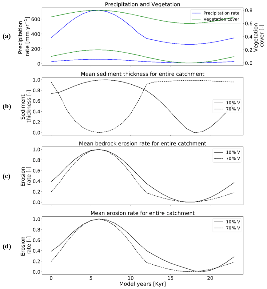
Figure A1Temporal evolution of catchment-averaged predictions for scenario 3 (with no weathering) described in the text (Sect. 3.3). Graphical representation of normalized mean catchment sedimentation and erosion to (a) coupled oscillations in precipitation [mm yr−1] and vegetation cover [–] in terms of (b) sediment thickness [–], (c) bedrock erosion [–], and (d) mean erosion rate [–] for the entire catchment. The periodicity of climate and vegetation oscillations is 23 kyr with a rock uplift rate of 0.5 mm yr−1.
Table A1Landscape evolution model input parameters used and corresponding units.
The code and data used in this study are freely available upon request.
HS and TAE designed the initial model setup and simulation programs. HS and TAE conducted model modifications, simulation runs, and analysis. MS provided assistance in program modification. KT provided insight into plant ecology in Chilean study areas and vegetation–climate change relationships. HS and TAE prepared the paper with contributions from CG, KT, and MS.
The authors declare that they have no conflict of interest.
Publisher's note: Copernicus Publications remains neutral with regard to jurisdictional claims in published maps and institutional affiliations.
Hemanti Sharma and Todd A. Ehlers acknowledge support from the Open Access Publishing Fund of the University of Tübingen. We also acknowledge support from the Research Training Group 1829 Integrated Hydrosystem Modelling, funded by the German Research Foundation (DFG). In addition, Todd A. Ehlers, Katja Tielbörger, and Manuel Schmid acknowledge support from the German priority research program (SPP-1803; grants EH329/14-1 and EH329/14-2 to Todd A. Ehlers; TI 338/14-1 and TI338/14-2 to Katja Tielbörger). We thank Erkan Istanbulluoglu and Omer Yetemen for their constructive reviews.
This research has been supported by the Deutsche Forschungsgemeinschaft (Research Training Group 1829 Integrated Hydrosystem Modelling, grant nos. SPP-1803, EH329/14-1, EH329/14-2, TI 338/14-1, and TI338/14-2).
This open-access publication was funded by the University of Tübingen.
This paper was edited by Greg Hancock and reviewed by Erkan Istanbulluoglu and Omer Yetemen.
Acosta, V. T., Schildgen, T. F., Clarke, B. A., Scherler, D., Bookhagen, B., Wittmann, H., von Blanckenburg, F., and Strecker, M. R.: Effect of vegetation cover on millennial-scale landscape denudation rates in East Africa, Lithosphere, 7, 408–420, https://doi.org/10.1130/l402.1, 2015.
Ahnert, F.: Some comments on the quantitative formulation of geomorphological processes in a theoretical model, Earth Surf. Process., 2, 191–201, https://doi.org/10.1002/esp.3290020211, 1977.
Alonso, R. N., Bookhagen, B., Carrapa, B., Coutand, I., Haschke, M., Hilley, G. E., Schoenbohm, L., Sobel, E. R., Strecker, M. R., Trauth, M. H., and Villanueva, A.: Tectonics, Climate, and Landscape Evolution of the Southern Central Andes: the Argentine Puna Plateau and Adjacent Regions between 22 and 30∘ S, in: The Andes: Active Subduction Orogeny, edited by: Oncken, O., Chong, G., Franz, G., Giese, P., Götze, H.-J., Ramos, V. A., Strecker, M. R., and Wigger, P., Springer, Berlin, Heidelberg, 265–283, 2006.
Amundson, R., Heimsath, A., Owen, J., Yoo, K., and Dietrich, W. E.: Hillslope soils and vegetation, Geomorphology, 234, 122–132, https://doi.org/10.1016/j.geomorph.2014.12.031, 2015.
Ashkenazy, Y., Eisenman, I., Gildor, H., and Tziperman, E.: The Effect of Milankovitch Variations in Insolation on Equatorial Seasonality, J. Climate, 23, 6133–6142, https://doi.org/10.1175/2010JCLI3700.1, 2010.
Avdievitch, N. N., Ehlers, T. A., and Glotzbach, C.: Slow Long-Term Exhumation of the West Central Andean Plate Boundary, Chile, Tectonics, 37, 2243–2267, https://doi.org/10.1029/2017TC004944, 2018.
Bellard, C., Bertelsmeier, C., Leadley, P., Thuiller, W., and Courchamp, F.: Impacts of climate change on the future of biodiversity, Ecol. Lett., 15, 365–377, https://doi.org/10.1111/j.1461-0248.2011.01736.x, 2012.
Bonnet, S. and Crave, A.: Landscape response to climate change: Insights from experimental modeling and implications for tectonic versus climatic uplift of topography, Geology, 31, 123–126, https://doi.org/10.1130/0091-7613(2003)031<0123:Lrtcci>2.0.Co;2, 2003.
Braun, J., Voisin, C., Gourlan, A. T., and Chauvel, C.: Erosional response of an actively uplifting mountain belt to cyclic rainfall variations, Earth Surf. Dynam., 3, 1–14, https://doi.org/10.5194/esurf-3-1-2015, 2015.
Breckle, S.-W.: Walter's Vegetation of the Earth, XX, 4th Edn., Springer-Verlag, Berlin, Heidelberg, 527 pp., 2002.
Collins, D. B. G., Bras, R. L., and Tucker, G. E.: Modeling the effects of vegetation-erosion coupling on landscape evolution, J. Geophys. Res., 109, F03004, https://doi.org/10.1029/2003jf000028, 2004.
Davy, P. and Lague, D.: Fluvial erosion/transport equation of landscape evolution models revisited, J. Geophys. Res., 114, F03007, https://doi.org/10.1029/2008jf001146, 2009.
Dixon, J. L., Heimsath, A. M., and Amundson, R.: The critical role of climate and saprolite weathering in landscape evolution, Earth Surf. Proc. Land., 34, 1507–1521, https://doi.org/10.1002/esp.1836, 2009.
Dosseto, A., Hesse, P. P., Maher, K., Fryirs, K., and Turner, S.: Climatic and vegetation control on sediment dynamics during the last glacial cycle, Geology, 38, 395–398, https://doi.org/10.1130/g30708.1, 2010.
Dunne, T., Malmon, D. V., and Mudd, S. M.: A rain splash transport equation assimilating field and laboratory measurements, J. Geophys. Res., 115, F01001, https://doi.org/10.1029/2009jf001302, 2010.
Fernandes, N. F. and Dietrich, W. E.: Hillslope evolution by diffusive processes: The timescale for equilibrium adjustments, Water Resour. Res., 33, 1307–1318, https://doi.org/10.1029/97wr00534, 1997.
Gerten, D., Luo, Y., Le Maire, G., Parton, W. J., Keough, C., Weng, E., Beier, C., Ciais, P., Cramer, W., Dukes, J. S., Hanson, P. J., Knapp, A. A. K., Linder, S., Nepstad, D., Rustad, L., and Sowerby, A.: Modelled effects of precipitation on ecosystem carbon and water dynamics in different climatic zones, Global Change Biol., 14, 2365–2379, https://doi.org/10.1111/j.1365-2486.2008.01651.x, 2008.
Gilbert, G. K.: Report on the geology of the Henry Mountains, US Government Printing Office, Washington, DC, https://doi.org/10.3133/70039916, 1877.
Hancock, G. S. and Anderson, R. S.: Numerical modeling of fluvial strath-terrace formation in response to oscillating climate, GSA Bull., 114, 1131–1142, https://doi.org/10.1130/0016-7606(2002)114<1131:NMOFST>2.0.CO;2, 2002.
Heimsath, A. M., Dietrich, W. E., Nishiizumi, K., and Finkel, R. C.: The soil production function and landscape equilibrium, Nature, 388, 358–361, https://doi.org/10.1038/41056, 1997.
Herman, F., Rhodes, E. J., Braun, J., and Heiniger, L.: Uniform erosion rates and relief amplitude during glacial cycles in the Southern Alps of New Zealand, as revealed from OSL-thermochronology, Earth Planet. Sc. Lett., 297, 183–189, https://doi.org/10.1016/j.epsl.2010.06.019, 2010.
Hobley, D. E. J., Adams, J. M., Nudurupati, S. S., Hutton, E. W. H., Gasparini, N. M., Istanbulluoglu, E., and Tucker, G. E.: Creative computing with Landlab: an open-source toolkit for building, coupling, and exploring two-dimensional numerical models of Earth-surface dynamics, Earth Surf. Dynam., 5, 21–46, https://doi.org/10.5194/esurf-5-21-2017, 2017.
Howard, A. D.: A detachment-limited model of drainage basin evolution, Water Resour. Res., 30, 2261–2285, https://doi.org/10.1029/94WR00757, 1994.
Huntley, B., Allen, J. R., Collingham, Y. C., Hickler, T., Lister, A. M., Singarayer, J., Stuart, A. J., Sykes, M. T., and Valdes, P. J.: Millennial climatic fluctuations are key to the structure of last glacial ecosystems, PLoS One, 8, e61963, https://doi.org/10.1371/journal.pone.0061963, 2013.
Huxman, T. E., Smith, M. D., Fay, P. A., Knapp, A. K., Shaw, M. R., Loik, M. E., Smith, S. D., Tissue, D. T., Zak, J. C., Weltzin, J. F., Pockman, W. T., Sala, O. E., Haddad, B. M., Harte, J., Koch, G. W., Schwinning, S., Small, E. E., and Williams, D. G.: Convergence across biomes to a common rain-use efficiency, Nature, 429, 651–654, https://doi.org/10.1038/nature02561, 2004.
Hyun, S., Ahagon, N., and Yoon, H.-I.: Milankovitch cycles and paleoceanographic evolution within sediments from ODP Sites 980 and 983 of the North Atlantic Ocean, Geosci. J., 9, 235–242, https://doi.org/10.1007/BF02910583, 2005.
Istanbulluoglu, E. and Bras, R. L.: Vegetation-modulated landscape evolution: Effects of vegetation on landscape processes, drainage density, and topography, J. Geophys. Res., 110, F02012, https://doi.org/10.1029/2004jf000249, 2005.
Istanbulluoglu, E. and Bras, R. L.: On the dynamics of soil moisture, vegetation, and erosion: Implications of climate variability and change, Water Resour. Res., 42, W06418, https://doi.org/10.1029/2005wr004113, 2006.
Jeffery, M. L., Yanites, B. J., Poulsen, C. J., and Ehlers, T. A.: Vegetation-precipitation controls on Central Andean topography, J. Geophys. Res.-Earth, 119, 1354–1375, https://doi.org/10.1002/2013jf002919, 2014.
Johnstone, S. A. and Hilley, G. E.: Lithologic control on the form of soil-mantled hillslopes, Geology, 43, 83–86, https://doi.org/10.1130/g36052.1, 2014.
Kelly, A. E. and Goulden, M. L.: Rapid shifts in plant distribution with recent climate change, P. Natl. Acad. Sci. USA, 105, 11823, https://doi.org/10.1073/pnas.0802891105, 2008.
Kirby, E. and Whipple, K. X.: Expression of active tectonics in erosional landscapes, J. Struct. Geol., 44, 54–75, https://doi.org/10.1016/j.jsg.2012.07.009, 2012.
Knapp, A. K., Ciais, P., and Smith, M. D.: Reconciling inconsistencies in precipitation–productivity relationships: implications for climate change, New Phytol., 214, 41–47, https://doi.org/10.1111/nph.14381, 2017.
Kojima, S., Soto, I., Quiroz, M., Valencia, P., and Fernandez, I.: Geological and Geochemical Characteristics of the Intrusion-Related Vein-Type Gold Deposits in the El Morado District, Coastal Cordillera, Northern Chile, Resour. Geol., 67, 197–206, https://doi.org/10.1111/rge.12129, 2017.
Lague, D., Crave, A., and Davy, P.: Laboratory experiments simulating the geomorphic response to tectonic uplift, J. Geophys. Res.-Solid, 108, ETG 3-1–ETG 3-20, https://doi.org/10.1029/2002jb001785, 2003.
Martin, Y.: Modelling hillslope evolution: linear and nonlinear transport relations, Geomorphology, 34, 1–21, https://doi.org/10.1016/S0169-555X(99)00127-0, 2000.
McPhillips, D., Bierman, P. R., Crocker, T., and Rood, D. H.: Landscape response to Pleistocene-Holocene precipitation change in the Western Cordillera, Peru: 10Be concentrations in modern sediments and terrace fills, J. Geophys. Res.-Earth, 118, 2488–2499, https://doi.org/10.1002/2013jf002837, 2013.
Melnick, D.: Rise of the central Andean coast by earthquakes straddling the Moho, Nat. Geosci., 9, 401–407, https://doi.org/10.1038/ngeo2683, 2016.
Miller, S. R., Sak, P. B., Kirby, E., and Bierman, P. R.: Neogene rejuvenation of central Appalachian topography: Evidence for differential rock uplift from stream profiles and erosion rates, Earth Planet. Sc. Lett., 369–370, 1–12, https://doi.org/10.1016/j.epsl.2013.04.007, 2013.
Mishra, A. K., Placzek, C., and Jones, R.: Coupled influence of precipitation and vegetation on millennial-scale erosion rates derived from 10Be, PLoS One, 14, e0211325, https://doi.org/10.1371/journal.pone.0211325, 2019.
Mowll, W., Blumenthal, D. M., Cherwin, K., Smith, A., Symstad, A. J., Vermeire, L. T., Collins, S. L., Smith, M. D., and Knapp, A. K.: Climatic controls of aboveground net primary production in semi-arid grasslands along a latitudinal gradient portend low sensitivity to warming, Oecologia, 177, 959–969, https://doi.org/10.1007/s00442-015-3232-7, 2015.
Oeser, R. A., Stroncik, N., Moskwa, L.-M., Bernhard, N., Schaller, M., Canessa, R., van den Brink, L., Köster, M., Brucker, E., Stock, S., Fuentes, J. P., Godoy, R., Matus, F. J., Oses Pedraza, R., Osses McIntyre, P., Paulino, L., Seguel, O., Bader, M. Y., Boy, J., Dippold, M. A., Ehlers, T. A., Kühn, P., Kuzyakov, Y., Leinweber, P., Scholten, T., Spielvogel, S., Spohn, M., Übernickel, K., Tielbörger, K., Wagner, D., and von Blanckenburg, F.: Chemistry and microbiology of the Critical Zone along a steep climate and vegetation gradient in the Chilean Coastal Cordillera, Catena, 170, 183–203, https://doi.org/10.1016/j.catena.2018.06.002, 2018.
Owen, J. J., Amundson, R., Dietrich, W. E., Nishiizumi, K., Sutter, B., and Chong, G.: The sensitivity of hillslope bedrock erosion to precipitation, Earth Surf. Proc. Land., 36, 117–135, https://doi.org/10.1002/esp.2083, 2011.
Pelletier, J. D.: Fluvial and slope-wash erosion of soil-mantled landscapes: detachment- or transport-limited?, Earth Surf. Proc. Land., 37, 37–51, https://doi.org/10.1002/esp.2187, 2012.
Perron, J. T.: Climate and the Pace of Erosional Landscape Evolution, Annu. Rev. Earth Planet. Sci., 45, 561–591, https://doi.org/10.1146/annurev-earth-060614-105405, 2017.
Rossel, K., Aguilar, G., Salazar, E., Martinod, J., Carretier, S., Pinto, L., and Cabré, A.: Chronology of Chilean Frontal Cordillera building from geochronological, stratigraphic and geomorphological data insights from Miocene intramontane-basin deposits, Basin Res., 30, 289–310, https://doi.org/10.1111/bre.12221, 2018.
Routschek, A., Schmidt, J., and Kreienkamp, F.: Impact of climate change on soil erosion – A high-resolution projection on catchment scale until 2100 in Saxony/Germany, Catena, 121, 99–109, https://doi.org/10.1016/j.catena.2014.04.019, 2014.
Sala, O. E., Parton, W. J., Joyce, L. A., and Lauenroth, W. K.: Primary Production of the Central Grassland Region of the United States, Ecology, 69, 40–45, https://doi.org/10.2307/1943158, 1988.
Schaller, M. and Ehlers, T. A.: Limits to quantifying climate driven changes in denudation rates with cosmogenic radionuclides, Earth Planet. Sc. Lett., 248, 153–167, https://doi.org/10.1016/j.epsl.2006.05.027, 2006.
Schaller, M., Blanckenburg, F. von, Hovius, N., Veldkamp, A., van den Berg, M. W., and Kubik, P. W.: Paleoerosion Rates from Cosmogenic 10Be in a 1.3 Ma Terrace Sequence: Response of the River Meuse to Changes in Climate and Rock Uplift, J. Geol., 112, 127–144, https://doi.org/10.1086/381654, 2004.
Schaller, M., Ehlers, T. A., Lang, K. A. H., Schmid, M., and Fuentes-Espoz, J. P.: Addressing the contribution of climate and vegetation cover on hillslope denudation, Chilean Coastal Cordillera (26∘–38∘ S), Earth Planet. Sc. Lett., 489, 111–122, https://doi.org/10.1016/j.epsl.2018.02.026, 2018.
Schaller, M., Dal Bo, I., Ehlers, T. A., Klotzsche, A., Drews, R., Fuentes Espoz, J. P., and van der Kruk, J.: Comparison of regolith physical and chemical characteristics with geophysical data along a climate and ecological gradient, Chilean Coastal Cordillera (26 to 38∘ S), Soil, 6, 629–647, https://doi.org/10.5194/soil-6-629-2020, 2020.
Schmid, M., Ehlers, T. A., Werner, C., Hickler, T., and Fuentes-Espoz, J.-P.: Effect of changing vegetation and precipitation on denudation – Part 2: Predicted landscape response to transient climate and vegetation cover over millennial to million-year timescales, Earth Syst. Dynam., 6, 859–881, https://doi.org/10.5194/esurf-6-859-2018, 2018.
Seybold, H., Rothman, D. H., and Kirchner, J. W.: Climate's watermark in the geometry of stream networks, Geophys. Res. Lett., 44, 2272–2280, https://doi.org/10.1002/2016gl072089, 2017.
Shobe, C. M., Tucker, G. E., and Barnhart, K. R.: The SPACE 1.0 model: a Landlab component for 2-D calculation of sediment transport, bedrock erosion, and landscape evolution, Geosci. Model Dev., 10, 4577–4604, https://doi.org/10.5194/gmd-10-4577-2017, 2017.
Slater, L. J. and Singer, M. B.: Imprint of climate and climate change in alluvial riverbeds: Continental United States, 1950–2011, Geology, 41, 595–598, https://doi.org/10.1130/g34070.1, 2013.
Smith, B., Wårlind, D., Arneth, A., Hickler, T., Leadley, P., Siltberg, J., and Zaehle, S.: Implications of incorporating N cycling and N limitations on primary production in an individual-based dynamic vegetation model, Biogeosciences, 11, 2027–2054, https://doi.org/10.5194/bg-11-2027-2014, 2014.
Smith, M. D., Wilcox, K. R., Power, S. A., Tissue, D. T., and Knapp, A. K.: Assessing community and ecosystem sensitivity to climate change – toward a more comparative approach, J. Veg. Sci., 28, 235–237, https://doi.org/10.1111/jvs.12524, 2017.
Starke, J., Ehlers, T. A., and Schaller, M.: Latitudinal effect of vegetation on erosion rates identified along western South America, Science, 367, 1358, https://doi.org/10.1126/science.aaz0840, 2020.
Tucker, G. E.: Drainage basin sensitivity to tectonic and climatic forcing: implications of a stochastic model for the role of entrainment and erosion thresholds, Earth Surf. Proc. Land., 29, 185–205, https://doi.org/10.1002/esp.1020, 2004.
Tucker, G. E., Lancaster, S. T., Gasparini, N. M., and Bras, R. L.: Modeling floodplain dynamics and stratigraphy: implications for geoarchaeology, Final Technical Report (Part II-C), Contract Number DACA88-95-C-0017, USACERL – US Army Corps of Engineers Construction Engineering Research Laboratory, 16 pp., 1999.
Tucker, G. E., Lancaster, S. T., Gasparini, N. M., Bras, R. L., and Rybarczyk, S. M.: An object-oriented framework for distributed hydrologic and geomorphic modeling using triangulated irregular networks, Comput. Geosci., 27, 959–973, https://doi.org/10.1016/S0098-3004(00)00134-5, 2001.
Turowski, J. M., Lague, D., Crave, A., and Hovius, N.: Experimental channel response to tectonic uplift, J. Geophys. Res.-Earth, 111, F03008, https://doi.org/10.1029/2005jf000306, 2006.
van Dongen, R., Scherler, D., Wittmann, H., and von Blanckenburg, F.: Cosmogenic 10Be in river sediment: where grain size matters and why, Earth Surf. Dynam., 7, 393–410, https://doi.org/10.5194/esurf-7-393-2019, 2019.
Werner, C., Schmid, M., Ehlers, T. A., Fuentes-Espoz, J. P., Steinkamp, J., Forrest, M., Liakka, J., Maldonado, A., and Hickler, T.: Effect of changing vegetation and precipitation on denudation – Part 1: Predicted vegetation composition and cover over the last 21 thousand years along the Coastal Cordillera of Chile, Earth Surf. Dynam., 6, 829–858, https://doi.org/10.5194/esurf-6-829-2018, 2018.
Whipple, K. X.: The influence of climate on the tectonic evolution of mountain belts, Nat. Geosci., 2, 730–730, https://doi.org/10.1038/ngeo638, 2009.
Whipple, K. X. and Tucker, G. E.: Dynamics of the stream-power river incision model: Implications for height limits of mountain ranges, landscape response timescales, and research needs, J. Geophys. Res.-Solid, 104, 17661–17674, https://doi.org/10.1029/1999jb900120, 1999.
Willgoose, G., Bras, R. L., and Rodriguez-Iturbe, I.: A coupled channel network growth and hillslope evolution model: 1. Theory, Water Resour. Res., 27, 1671–1684, https://doi.org/10.1029/91WR00935, 1991.
Xia, J., Chen, J., Piao, S., Ciais, P., Luo, Y., and Wan, S.: Terrestrial carbon cycle affected by non-uniform climate warming, Nat. Geosci., 7, 173–180, https://doi.org/10.1038/ngeo2093, 2014.
Yang, Y., Fang, J., ma, W., and Wang, W.: Relationship between variability in aboveground net primary production and precipitation in global grasslands. Geophys. Res. Lett., 35, L23710, https://doi.org/10.1029/2008GL035408, 2008.
Yanites, B. J. and Ehlers, T. A.: Global climate and tectonic controls on the denudation of glaciated mountains, Earth Planet. Sc. Lett., 325–326, 63–75, https://doi.org/10.1016/j.epsl.2012.01.030, 2012.
Yetemen, O., Istanbulluoglu, E., and Duvall, A. R.: Solar radiation as a global driver of hillslope asymmetry: Insights from an ecogeomorphic landscape evolution model, Water Resour. Res., 51, 9843–9861, https://doi.org/10.1002/2015WR017103, 2015.
Yetemen, O., Saco, P. M., and Istanbulluoglu, E.: Ecohydrology Controls the Geomorphic Response to Climate Change, Geophys. Res. Lett., 46, 8852–8861, https://doi.org/10.1029/2019GL083874, 2019.
Zhang, Y., Xiao, X., Guanter, L., Zhou, S., Ciais, P., Joiner, J., Sitch, S., Wu, X., Nabel, J., Dong, J., Kato, E., Jain, A. K., Wiltshire, A., and Stocker, B. D.: Precipitation and carbon-water coupling jointly control the interannual variability of global land gross primary production, Scient. Rep., 6, 39748, https://doi.org/10.1038/srep39748, 2016.