Reconstructing the dynamics of the highly similar May 2016 and June 2019 Iliamna Volcano (Alaska) ice–rock avalanches from seismoacoustic data

Surficial mass wasting events are a hazard worldwide. Seismic and acoustic signals from these often remote processes, combined with other geophysical observations, can provide key information for monitoring and rapid response efforts and enhance our understanding of event dynamics. Here, we present seismoacoustic data and analyses for two very large ice–rock avalanches occurring on Iliamna Volcano, Alaska (USA), on 22 May 2016 and 21 June 2019. Iliamna is a glacier-mantled stratovolcano located in the Cook Inlet, ∼200 km from Anchorage, Alaska. The volcano experiences massive, quasi-annual slope failures due to glacial instabilities and hydrothermal alteration of volcanic rocks near its summit. The May 2016 and June 2019 avalanches were particularly large and generated energetic seismic and infrasound signals which were recorded at numerous stations at ranges from ∼9 to over 600 km. Both avalanches initiated in the same location near the head of Iliamna's east-facing Red Glacier, and their ∼8 km long runout shapes are nearly identical. This repeatability – which is rare for large and rapid mass movements – provides an excellent opportunity for comparison and validation of seismoacoustic source characteristics. For both events, we invert long-period (15–80 s) seismic signals to obtain a force-time representation of the source. We model the avalanche as a sliding block which exerts a spatially static point force on the Earth. We use this force-time function to derive constraints on avalanche acceleration, velocity, and directionality, which are compatible with satellite imagery and observed terrain features. Our inversion results suggest that the avalanches reached speeds exceeding 70 m s⁻¹, consistent with numerical modeling from previous Iliamna studies. We lack sufficient local infrasound data to test an acoustic source model for these processes. However, the acoustic data suggest that infrasound from these avalanches is produced after the mass movement regime transitions from cohesive block-type failure to granular and turbulent flow – little to no infrasound is generated by the initial failure. At Iliamna, synthesis of advanced numerical flow models and more detailed ground observations combined with increased geophysical station coverage could yield significant gains in our understanding of these events.

1 Introduction

Surficial gravitational mass movements, such as debris flows, rockfalls, lahars, and avalanches, constitute a broad collection of Earth processes which are a significant hazard around the world (Voight, 1978). These events can cause devastating damage to life and property when they occur in at-risk, populated areas in mountainous regions or on the flanks of volcanoes. Avalanches involving mixtures of ice and rock are a subset of these processes usually occurring in topographically extreme, glaciated terrain. Some of the most deadly surficial gravitational mass movements (hereafter, just “mass movements”) in history were ice–rock avalanches. For example, the Huascarán avalanches occurring in 1962 and 1970 in the Peruvian Andes together claimed an estimated 22 000 lives (Plafker and Ericksen, 1978). However, due to their high mobility and frequently remote location, eyewitness observations of these dramatic processes are rare (Caplan-Auerbach and Huggel, 2007; Coe et al., 2016), and other assessment methods such as geologic mapping or satellite imagery analysis may not be timely or even possible due to the rugged terrain and volatile mountain weather typically found in such settings.

Seismoacoustics is an emerging tool which can help us understand these powerful yet elusive processes (Allstadt et al., 2018, and references therein). Mass movements transfer energy into the solid Earth as seismic waves and into the atmosphere as acoustic waves. The atmospheric waves are primarily in the infrasonic range at frequencies below the range of human hearing (<20 Hz). These signals contain valuable and complementary information about the character and size of the event and also provide a high-resolution record of event timing. Most mass movements large enough to be destructive can be recorded seismoacoustically from sufficiently safe distances. By analyzing the seismic and acoustic waves generated by these processes, we can better understand their dynamics and work towards improved hazard mitigation and response. Seismology and infrasound are, therefore, some of the most promising tools for near-real-time detection and characterization of remote mass movements (Allstadt et al., 2018). However, development of detailed seismoacoustic source models is still an area of active research, as relatively few well-recorded events – particularly those with both seismic and infrasound data – exist.

Here, we focus on two ice–rock avalanches that occurred in May 2016 and June 2019 on Iliamna Volcano, Alaska, USA. These avalanches were very large, each measuring ∼8 km from crown to toe. Both events produced energetic seismic and acoustic signals broadly recorded at local (<100 km) and regional (>100 km) distances. Relatively dense regional seismic and acoustic networks were in place during these events (Fig. 1), providing a unique opportunity for source quantification and comparison. Additionally, the location and nature of failure and the material, shape, and size of the resulting deposits are very similar between the two events (Fig. 2), providing excellent datasets for comparison. Iliamna Volcano is known for frequent, large mass movements of this nature (e.g., Caplan-Auerbach et al., 2004; Caplan-Auerbach and Huggel, 2007; Huggel et al., 2007; Schneider et al., 2010).

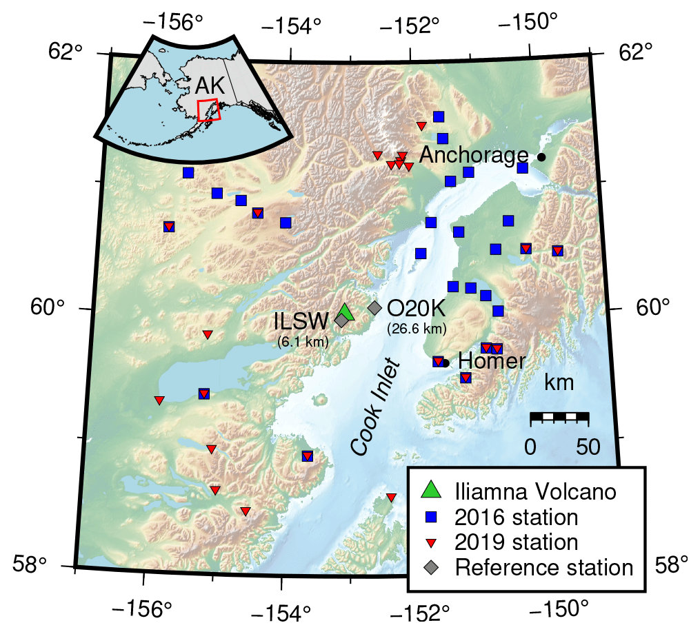
Figure 1 Map of the Cook Inlet region, Alaska. Iliamna Volcano is indicated by the green triangle. Broadband seismic stations used in the 2016 (28 stations) and 2019 (23 stations) force inversions are shown as blue squares and red inverted triangles, respectively. Overlapping markers denote stations used in both inversions. The station distribution varies greatly between the two events due to the presence of a temporary seismic array in 2016 and increased Transportable Array station coverage in 2019. Reference stations ILSW and O20K (the closest seismometer and infrasound sensor to the events, respectively) are shown as gray diamonds with their distances to Iliamna Volcano given in parentheses. The city of Anchorage and the town of Homer are marked as black dots. The red box in the inset shows the main map extent.

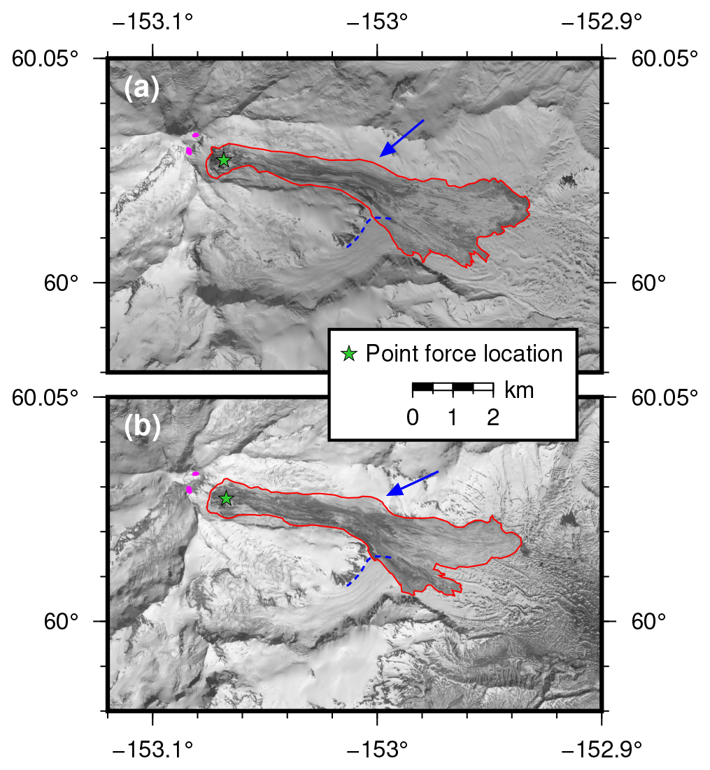
Figure 2 Satellite images of the 2016 and 2019 Red Glacier avalanche deposits acquired on (a) 23 May 2016 and (b) 22 June 2019, both less than 48 h post-event. Red outlines delineate approximate avalanche extents (source, track, and deposit areas). Green stars mark the location of the inversion point force. Blue arrows indicate the location of superelevation-like flow lobes. Blue dashed lines delineate the northern margin of an unnamed tributary glacier which joins Red Glacier from the southwest. Magenta patches show the approximate locations of two fumarole zones located to the east of the summit. Imagery © 2016 and 2019 Planet Labs, Inc.

In this study, we describe the acoustic and seismic signals generated by the 2016 and 2019 Iliamna Volcano avalanches, along with auxiliary information including aerial, ground-based, and satellite imagery. We explore the timing and strength of the avalanche acoustic signal and assess the possibility of acoustic source directionality. We invert the strong long-period seismic signals produced by the events to obtain the time series of forces that the center of mass (COM) of each avalanche exerted on the Earth – the “force-time function”. From there, we calculate the acceleration, velocity, and displacement of the COMs and compare these to auxiliary data such as digital elevation models and satellite imagery. Our modeled forces and trajectories generally agree well with the satellite imagery and observed terrain features and offer insight into the seismoacoustic source properties of these massive avalanches.

2 Background

2.1 Analysis of long-period seismic waves from mass movements

The amplitude and frequency content of the seismic wave field radiated by a surficial mass movement are strongly controlled by the spatial and temporal scales involved as well as the structural coherence of the moving material. Processes such as powdery snow avalanches and lahars, which primarily involve incoherent collections of fine-grained particles, produce relatively high-frequency seismicity (Allstadt et al., 2018). However, larger events which move coherently – such as rockfalls and ice–rock avalanches – can additionally produce significant long-period (>10 s) seismic energy that can be recorded globally (Hibert et al., 2017; Allstadt et al., 2018). These long-period seismic waves originate from the bulk acceleration and deceleration of the mass as it moves downslope (Ekström and Stark, 2013).

Long-period seismic waves can be used to invert for quantitative mass movement source properties. The wave propagation (i.e., Green's function) at these periods is often straightforward to model due to the relatively small influence of topography and Earth structure on such long-wavelength signals. Once the propagation is accounted for, one can invert for the time-varying force vector that the moving mass exerted on the Earth (e.g., Kawakatsu, 1989; Allstadt, 2013; Ekström and Stark, 2013; Coe et al., 2016; Gualtieri and Ekström, 2018). The trajectory can then be obtained if the mass, generally assumed to be constant, is known or can be estimated (e.g., Ekström and Stark, 2013; Moore et al., 2017; Gualtieri and Ekström, 2018; Schöpa et al., 2018). However, complexities such as entrainment and deposition along the flow path clearly violate the constant mass approximation, so this method has generally only been successful for simple runout paths. The infrequent nature of mass movements capable of generating sufficiently long-period seismic radiation means that opportunities to apply this model are limited (Hibert et al., 2017).

2.2 Acoustic studies of mass movements

More recently, studies have incorporated observations and analysis of infrasound generated by mass movements. Because infrasound stations are often deployed in volcano-monitoring settings (Fee and Matoza, 2013; Matoza et al., 2019), many acoustic observations of mass movements have documented volcanic phenomena such as pyroclastic flows (e.g., Yamasato, 1997; Ripepe et al., 2009, 2010; Delle Donne et al., 2014), lahars (e.g., Johnson and Palma, 2015), rockfalls (e.g., Moran et al., 2008; Johnson and Ronan, 2015), and flank collapse events (e.g., Perttu et al., 2020). Outside of the volcanic context, debris flows (e.g., Kogelnig et al., 2014; Schimmel and Hübl, 2016; Marchetti et al., 2019), powder snow avalanches, (e.g., Ulivieri et al., 2011; Havens et al., 2014; Marchetti et al., 2015, 2020), nonvolcanic rockfalls (e.g., Zimmer et al., 2012; Zimmer and Sitar, 2015), and rock avalanches (e.g., Moore et al., 2017) have been observed acoustically. Infrasound recordings of surficial mass flows at regional distances are rare.

Infrasonic source directionality has previously been assessed for dense recordings of volcanic explosions. For example, Iezzi et al. (2019) performed a multipole acoustic source inversion on explosions from Yasur Volcano, Vanuatu, describing the source as a combination of monopole (uniform radiation) and dipole (directional radiation) components. Mass movement acoustic radiation has been suggested to be highly directional and potentially described by an acoustic dipole (Allstadt et al., 2018; Haney et al., 2018). However, assessment of acoustic source directionality for mass movements requires dense station coverage, which is not usually available (Iezzi et al., 2019); therefore, the actual source directionality has not been validated with data. Additionally, beyond local distances, path effects from the usually highly spatiotemporally variable atmosphere become important. These effects can mask source directionality or produce spurious source directionality and must be considered in analyses (e.g., Perttu et al., 2020).

Arrays of infrasound sensors can be used to determine the back azimuth of incident acoustic waves and can track flow fronts under certain circumstances (e.g., Johnson and Palma, 2015; Marchetti et al., 2020). Although infrasonic records of mass movements are becoming more common, the relevant acoustic source theory is currently underdeveloped (Allstadt et al., 2018). Very simple mass movements such as rockfalls have been treated as monopoles (e.g., Moran et al., 2008), but often the source of infrasound is moving and distributed, complicating modeling. Marchetti et al. (2019) modeled a debris flow as a linear series of monopole sources in motion, but found that infrasound array processing results always pointed back to fixed locations corresponding to check dams in the debris flow drainage, the most acoustically energetic sources. Using infrasound arrays, Johnson and Palma (2015) tracked a lahar which registered as a moving source until it encountered a topographic notch, at which point the source location became fixed on this acoustically “loud” flow feature. The dynamic, spatiotemporal variability of the atmosphere also complicates infrasound source modeling (Poppeliers et al., 2020). These studies highlight the challenge in determining the source of mass-movement-generated infrasound.

2.3 Ice–rock avalanches

Ice–rock avalanches are a subset of mass movements which consist of rapid flows of pulverized ice and rock. Though the initial failure of an ice–rock avalanche can free larger blocks of material, such blocks quickly disintegrate into small fragments of rock and ice as they impact asperities in the flow path at speed. This debris travels on a saturated, low-strength layer of material, increasing avalanche mobility (Hungr et al., 2014). Additionally, because these processes often take place in steep, heavily glaciated terrain (Schneider et al., 2011), the avalanches commonly flow over glaciers. This further enhances mobility due to the low friction of glacier ice (Schneider et al., 2010). Debris avalanches involving volcanic rocks can be especially mobile due to the weakened edifice rock of which they are composed, which more readily transforms to low-internal-friction granular flow (Davies et al., 2010). Owing to their high mobility and often large volumes (Schneider et al., 2011; Hungr et al., 2014), debris avalanches such as ice–rock avalanches are among the most seismogenic types of mass movements (Allstadt et al., 2018).

2.4 Iliamna Volcano, Alaska

Iliamna Volcano (hereafter, “Iliamna”) is a 3053 m tall stratovolcano located in the Cook Inlet region of south-central Alaska, USA (Fig. 1). The volcano lies about 215 km from the city of Anchorage, and roughly 100 km across the Cook Inlet from the town of Homer. The geology of Iliamna consists primarily of stratified andesitic lava flows with smaller contributions from mass wasting deposits of various types. The volcano's summit is perennially mantled with snow and ice, and its edifice hosts several large valley glaciers (Waythomas and Miller, 1999). Two zones of sulfurous fumaroles located on the eastern side of Iliamna's summit (see magenta patches in Fig. 2) emit steam and volcanic gas quasi-continuously (Werner et al., 2011).

Although Iliamna has not erupted in historical time, it experienced two periods of seismic unrest occurring in 1996 and 2012, which were interpreted as magmatic intrusions and failed eruptions (Roman et al., 2004; Herrick et al., 2014). Additionally, the deeply dissected and hydrothermally altered edifice of Iliamna hosts frequent mass wasting events. Geologic evidence of late Holocene lahars and debris avalanches is abundant (Waythomas et al., 2000), and Iliamna has experienced at least 12 very large (horizontal runout length L>5 km) ice–rock avalanches since 1960 (Huggel et al., 2007; Allstadt et al., 2017). A total of 10 of these 12 events occurred on Iliamna's east-facing Red Glacier. These avalanches typically fail in ice or at the ice–bedrock interface near the base of the hydrothermally altered fumarole zones near the summit. The avalanches are relatively frequent, with a recurrence interval of 2–4 years. This interval may be linked to the “recharging” time required for ice thickness to grow until shear stress exceeds shear strength (Huggel et al., 2007).

Iliamna's ice–rock avalanches have been extensively studied via geologic mapping, multispectral satellite image analysis, numerical modeling, and seismic analysis. Geologic investigations by Waythomas et al. (2000) revealed that late Holocene debris avalanche deposits composed of hydrothermally altered rock are present in most of Iliamna's glacier-filled valleys. From the thin, blanket-like appearance of these deposits, Waythomas et al. (2000) inferred that the original avalanches likely contained a significant amount of snow or ice in addition to rock. Caplan-Auerbach et al. (2004) documented the seismic signals associated with four very large Iliamna ice–rock avalanches. They found the signals to be remarkably similar, each exhibiting a precursory pattern of 20–60 min of repeating discrete events which become closer together in time, culminating with a high-amplitude emergent-onset waveform corresponding with the actual failure. This precursory phenomenon was explored further by Caplan-Auerbach and Huggel (2007), who defined four phases of precursory activity:

1. crevasse opening, with minimal seismic energy release;

2. acceleration of glacier movement;

3. discrete slipping, manifested as repeating seismogenic stick-slip events;

4. continuous slipping, which begins about 0.5–1 h prior to failure.

Caplan-Auerbach and Huggel (2007) also suggested that Iliamna's glaciers are affected by volcanogenic heating, enabling them to fail on slopes shallower than the 45^∘ threshold broadly assumed to be the minimum slope for cold-ice failure (Huggel et al., 2004). Huggel et al. (2007) found that satellite-derived thermal anomalies in Iliamna's summit region were spatially correlated with zones of fumarolic activity and hydrothermally altered rocks. Huggel et al. (2007) and Schneider et al. (2010) used successively more sophisticated numerical flow models to reconstruct a very large 2003 Red Glacier avalanche. Both studies were able to recreate flow features persistently observed for Red Glacier events since 1960, such as multiple distal flow lobes (toes) and prominent superelevation-like flow lobes on the orographically downslope left side of the flow.

3 Data

On 22 May 2016 at 07:58 UTC (about midnight local time; hereafter, all times in UTC unless otherwise noted), the Alaska Volcano Observatory (AVO) recorded emergent-onset seismic signals across Iliamna's local monitoring network, and a subsequent pilot report confirmed that a large mass movement had occurred. A Landsat 8 image acquired the following day revealed a large dark-colored deposit on Red Glacier; this deposit was also visible from Homer (Fig. 3a). A horizontal crown-to-toe runout length L of 8.5 km and a vertical drop height H of 1.7 km were estimated from follow-up imagery analysis, resulting in an $H/L$ ratio of 0.2.

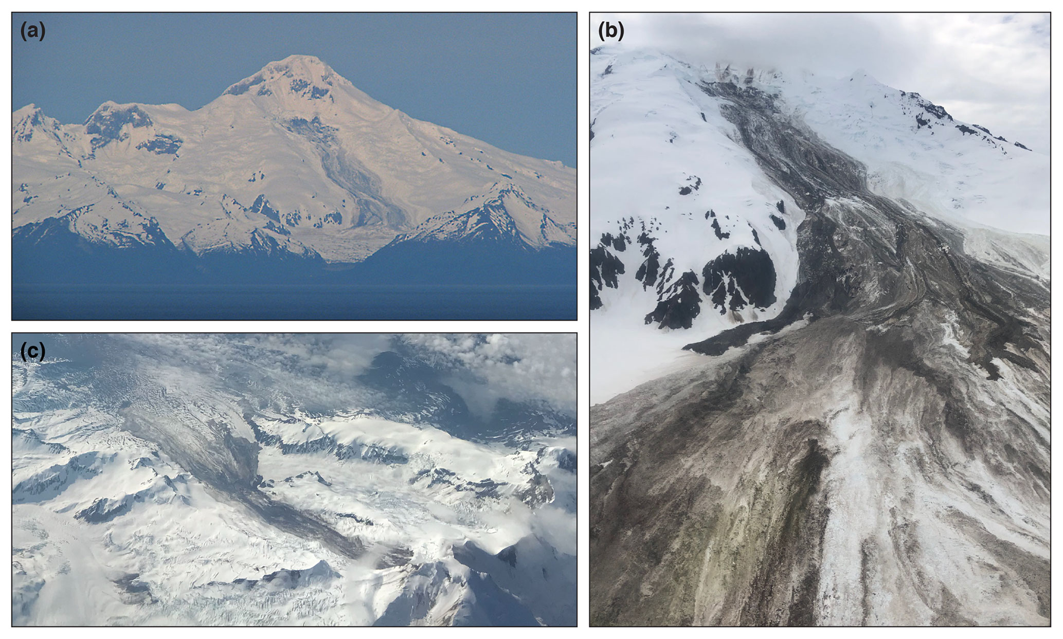
Figure 3 Photographs of the 2016 and 2019 Red Glacier avalanche deposits. (a) West-northwest-looking photograph of the 2016 deposit taken from near Homer on 23 May 2016. Photo courtesy of Dennis Anderson, Night Trax Photography; Alaska Volcano Observatory (AVO) image database ID https://avo.alaska.edu/images/image.php?id=95521 (last access: March 2021). (b) West-northwest-looking aerial photograph of the 2019 deposit, taken 22 June 2019. Photo courtesy of Loren Prosser; AVO image database ID https://avo.alaska.edu/images/image.php?id=140871 (last access: March 2021). (c) Southeast-looking aerial photograph of the 2019 deposit, taken 25 June 2019. Photo courtesy of Greg Johnson; AVO image database ID https://avo.alaska.edu/images/image.php?id=141431 (last access: March 2021).

On 21 June 2019 at 00:03, AVO recorded signals on Iliamna's seismic network indicative of another large avalanche. Photos from citizen overflights taken in the following several days (Fig. 3b, c) showed a large deposit on Red Glacier. Satellite imagery analysis produced values of L=8.1 km and H=1.7 km ($H/L$ ratio of 0.2). The combined source, track, and deposit areas for these two avalanches are delineated in Fig. 2.

The 2016 and 2019 Iliamna ice–rock avalanches are well-documented due to the relatively accessible nature of the volcano – by Alaskan standards – as well as the exceptional instrument coverage afforded by several permanent and temporary seismoacoustic networks. Our seismoacoustic observations and interpretations were assisted by high-resolution (meter-scale, daily revisit) satellite imagery, aerial and ground-based imagery acquired fortuitously or opportunistically in the days following the events, and high-resolution (sub-meter-scale) elevation data.

3.1 Seismic signals

Seismic signals from the events were broadly recorded on local and regional networks. Stations in the EarthScope USArray Transportable Array (network code TA), AVO (network code AV; Power et al., 2020), and Alaska Earthquake Center (AEC; network code AK) networks recorded signals from both events. The temporary Southern Alaska Lithosphere and Mantle Observation Network (SALMON; network code ZE; Tape et al., 2017), which was deployed from 2015 to 2017, captured the 2016 event. Additionally, stations in the National Tsunami Warning Center (network code AT), temporary Alaska Amphibious Community Seismic Experiment (network code XO), and Global Seismograph Network (GSN; network code II) networks recorded one or both of the events. Most stations which recorded the signal were broadband (120 s corner period) three-component sensors.

AVO station ILSW, at ∼ 6 km from the avalanche crowns (Fig. 1), was the closest seismometer with usable data in both 2016 and 2019. We note here that due to the size and mobility of these avalanches, source-to-station distances change drastically over the course of the event; ILSW is ∼ 12 km from the toes of the deposits. Vertical-component spectrograms and waveforms of avalanche seismic signals recorded at this station are shown in Fig. 4. Multiple high-frequency transients are visible in the spectrograms prior to the main event, indicative of precursory stick-slip activity which has been observed for previous Red Glacier avalanches and is thoroughly explored in Caplan-Auerbach and Huggel (2007). The main event waveforms have an emergent onset characteristic of mass movement seismic signals (Allstadt et al., 2018). This same shape, albeit with a lower signal-to-noise ratio (SNR), is found at all stations which recorded the event. The events also produced prodigious long-period energy with a dominant period of 35 s (Fig. 5). In this paper we do not analyze the precursory stick-slip activity observed for the 2016 and 2019 avalanches.

Figure 4 Vertical-component spectrograms (a, b) and seismic waveforms (c, d) from Alaska Volcano Observatory station ILSW for the 2016 (a, c) and 2019 (b, d) avalanches. Waveforms are high-pass filtered at 100 s.

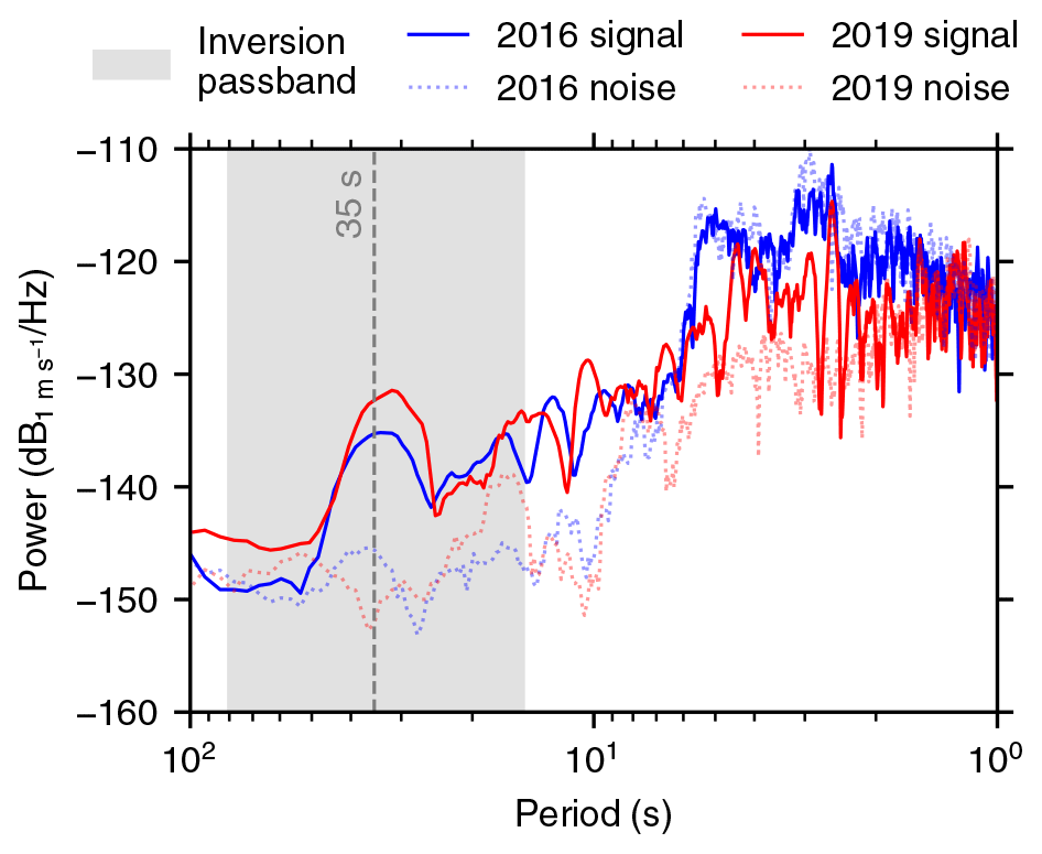
Figure 5 Power spectral densities (PSDs) of vertical-component seismic signals from the 2016 (blue lines) and 2019 (red lines) avalanches. The signals were recorded at Alaska Earthquake Center station HOM, the closest station to Iliamna Volcano used in both force inversions. Dotted lines are the PSDs for a 1000 s post-avalanche time window and indicate the approximate contemporaneous noise level. The gray box indicates the force inversion passband (15–80 s).

3.2 Acoustic signals

The 2016 and 2019 events produced strong infrasound signals which were recorded out to distances exceeding 600 km (Fig. 6). Signals were observed on select infrasound “single station” sensors of the TA, GSN, and AEC networks, as well as regional arrays operated by AVO and one International Monitoring System (network code IM) array. The nearest infrasound sensor at the time was TA station O20K (Fig. 1) at ∼ 19 and ∼ 26 km from the avalanche toes and crowns, respectively.

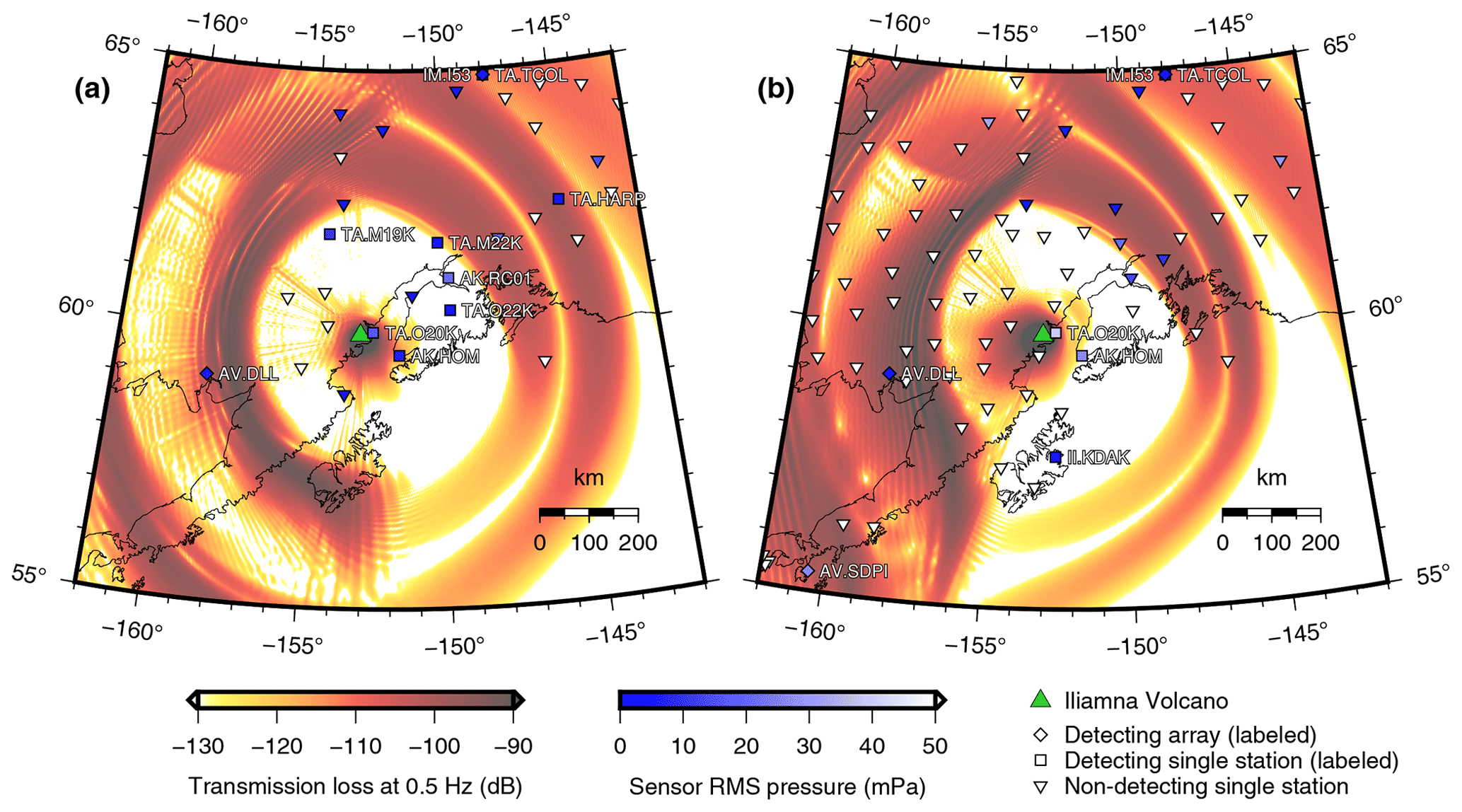
Figure 6 Acoustic transmission loss at the Earth's surface, modeled at 0.5 Hz for the (a) 2016 and (b) 2019 avalanches. The atmospheric model is a single sonde (1D atmospheric profile) over the avalanche path midpoint. Iliamna Volcano is indicated by the green triangle. Diamonds and squares denote the respective arrays and stations where the avalanche signal was detected. Inverted triangles indicate other infrasound stations where no signal was observed. The blue shades on the station markers indicate root-mean-square (RMS) pressure in the 0.5–2 Hz band for hour-long windows prior to the predicted true arrival. This is a proxy for local site noise. (See Sect. 3 for description of network codes.)

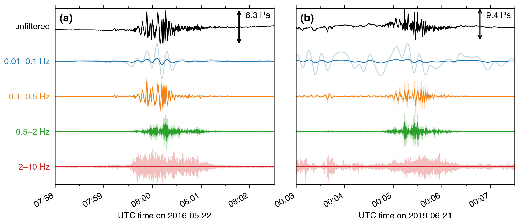
Figure 7 Infrasound signals in different frequency bands for the (a) 2016 and (b) 2019 avalanches. Signals were recorded on Transportable Array station O20K, the closest infrasound sensor to Iliamna Volcano at the time. Signals plotted as solid lines are normalized relative to the black unfiltered trace. Translucent lines are individually normalized signals.

“Waterfall” plots of the infrasound signal at station O20K in different frequency bands for the 2016 and 2019 events are shown in Fig. 7 and illustrate the signal's broadband nature. The dominant frequency of the signal is about 0.5 Hz, but energy exists from 100 s up to 10 Hz (the Nyquist frequency for this station). In 2016, the ∼ 120 s duration of the high-frequency signal (2–10 Hz, red line) is nearly twice that of the longer-period signal (0.01–0.1 Hz, blue line). The 2016 and 2019 signals are of similar amplitudes, but in 2019 the noise level is higher in the 0.01–0.1 and 2–10 Hz bands (Fig. 7b).

3.3 Aerial photos, satellite imagery, and elevation data

We interpret image data from three sources to augment our waveform-based analyses. Our satellite image sources are the Planet Labs PlanetScope (3 m resolution) and RapidEye (5 m resolution) satellite constellations and the DigitalGlobe WorldView-3 (WV-3, sub-meter resolution) satellite. We use the near-infrared band (NIR) from Planet Labs images acquired less than 48 h following each event (23 May 2016 and 22 June 2019) to constrain the dimensions of the source and deposit areas for each avalanche (Fig. 2). Fortunately, cloud cover was minimal during this time window. A panchromatic WV-3 image from 22 June 2016 captured the finer details of the source and deposit, although we note that melting of the icy portion of the deposit as well as additional smaller mass movements during the month between the 2016 avalanche and acquisition of the WV-3 image complicate our analysis of the image.

The 2016 and 2019 deposits were readily visible from Homer (Fig. 3a). Members of the community captured oblique aerial photos of the 2019 event during flyovers on 22 and 25 June 2019 (Fig. 3b, c). Additionally, in late July 2019, National Park Service and AVO staff flew a structure-from-motion (SfM) mission in the area around Iliamna, capturing about 4400 photos of the edifice and Red Glacier areas that were used to produce a 70 cm resolution digital elevation model (DEM). The DEM extent completely covers the total areas of both events. We use this DEM in our analysis with the caveat that the surface of Red Glacier is highly dynamic due to erosion from mass movements as well as glacial activity; therefore, the DEM is more applicable to the 2019 event than the 2016 event.

4 Methods

4.1 Mass estimation

We use the satellite imagery shown in Fig. 2 to estimate the mass for each event. We are unable to perform DEM subtraction to obtain a volume for either event due to insufficient data. Instead, we delineate the depositional area and assume a uniform (1.5 ± 1) m deposit thickness everywhere on the slope to obtain a volume. Red Glacier avalanche deposits are typically on the order of a few meters thick (Waythomas et al., 2000; Huggel et al., 2007), so this represents a reasonable estimate. We then multiply this volume by the density of a mixture of 50 % ice (density 920 kg m⁻³) and 50 % rock (density 2500 kg m⁻³) to obtain mass estimates. This assumed mixture is based upon the color of the deposits seen in Fig. 2 as well as the composition inferred for previous Red Glacier avalanches (Waythomas et al., 2000).

4.2 Infrasound analyses

Infrasound signals travel in atmospheric waveguides created primarily by vertical gradients in temperature and horizontal winds (Drob et al., 2003). The presence or absence of such waveguides in a given propagation direction from the source strongly controls our ability to detect and characterize infrasonic signals (Fee et al., 2013). Furthermore, cultural and natural noise, especially locally sourced wind noise, can obscure a true signal. Just as in seismology, our goal for source studies is to isolate source properties from path and station effects. To achieve this for the Iliamna avalanches, we model infrasound propagation conditions and assess station noise levels for time periods surrounding each event.

4.2.1 Propagation modeling

We use the AVO-G2S (ground-to-space) open-source atmospheric specification (https://github.com/usgs/volcano-avog2s (last access: March 2021); Schwaiger et al., 2019) to examine infrasound propagation from the avalanches. We extract a 1D atmospheric profile above the avalanche path midpoint for the forecast hours of 22 May 2016 08:00 and 21 June 2019 00:00. AVO-G2S smoothly merges lower-atmosphere numerical weather prediction (NWP) products with upper-atmosphere empirical climatologies. We use the ERA5 NWP model from the European Centre for Medium-Range Weather Forecasts. The upper-atmosphere winds and temperature in AVO-G2S are defined by the 2014 update to the Horizontal Wind Model (Drob et al., 2015) and the NRLMSISE-00 atmospheric model, respectively. The output 1D profile defines temperature, zonal (east–west) and meridional (north–south) winds, density, and pressure as a function of altitude.

We then use the aforementioned profiles and the Modess code from ncpaprop (https://github.com/chetzer-ncpa/ncpaprop (last access: March 2021); Waxler et al., 2017) to model infrasonic transmission loss on the Earth's surface in the region around Iliamna. The transmission loss (TL) is the accumulated sound pressure loss as a function of range and height, expressed in decibels (dB). The Modess code solves a generalized Helmholtz equation for the propagation of a monochromatic pulse in a stratified (i.e., 1D) atmosphere. The method of normal modes is used to solve the equation, which uses the “effective sound speed approximation” – that is, the sum of the static sound speed and the along-path contribution of the horizontal wind field define the effective sound speed. We choose a 0.5 Hz frequency for modeling, because that is the dominant frequency of the observed acoustic signal, and we set the source height at 900 m, the approximate elevation of the midpoint of the avalanche paths. We compute the surface acoustic TL in decibels from 0–1000 km range for azimuths of 0–360^∘ in 1^∘ increments. We then map the data from range–azimuth space (with the origin being Iliamna) to longitude–latitude on the WGS84 ellipsoid and grid the result to produce continuous TL maps for the two events (Fig. 6).

4.2.2 Noise characterization

To assess the effect of local station noise on signal detection for single infrasound stations, we compute root-mean-square (RMS) pressure in the 0.5–2 Hz band on hour-long windows for each infrasound-equipped station within 900 km of Iliamna (see blue color scale in Fig. 6). We remove the instrument response, detrend, and taper the data prior to filtering. Windows are defined to sample the data in the hour immediately preceding signal arrival at a given station to avoid possible upwards biasing of extremely quiet stations by the avalanche signal itself. This is guaranteed by specifying a maximal acoustic celerity (distance/travel time) of 350 m s⁻¹ to define the moveout of the window end time. We remove stations with excessive glitches or dead channels (five stations in 2016; three stations in 2019).

4.3 Force inversions

We invert the long-period seismic signals generated by these events to obtain the time-varying forces that the avalanche COMs exerted on the Earth. We use a version of the approach detailed in Allstadt (2013) and applied in Coe et al. (2016). We model the avalanche as a block sliding down a slope experiencing a net force given by the balance between the slope-parallel gravitational and dynamic friction forces. By Newton's second law, this net force is equal and opposite to the time-varying force that the avalanche COM exerts on the Earth (Allstadt, 2013). In our model, this avalanche “force-time function” is applied to the Earth as a spatially static point force, which is valid for long-wavelength signals where the shift in source location due to mass motion is small relative to the signal wavelength. We define the point force location to be the COM of the avalanche source region (see Sect. 4.3.3 and the green stars in Fig. 2).

4.3.1 Data selection

We use data from seismic stations within 80–200 km of Iliamna. We omit all stations less than 80 km from the source because we know from satellite imagery that the COM locations for both avalanches moved up to 8 km. This constraint ensures that we only use stations for which the source-to-station distance changed by a maximum amount of 10 % over the course of the event, allowing us to consider the landslide source as a point force. Limiting our station search to 200 km results in a data volume sufficient to constrain the source yet small enough to make manual signal inspection feasible. Prior to inspection, waveforms were detrended using a second-order polynomial and rotated into the vertical–radial–transverse (Z–R–T) reference frame. We additionally deconvolve the instrument response to obtain units of displacement and apply a 15–80 s bandpass filter. The passband was selected to avoid noise associated with the secondary microseism (3–10 s; Gualtieri et al., 2015) and to ensure that the maximum period of the filtered signals is below the corner period of the seismometers used. After this processing, we select waveforms with sufficient SNR by visual inspection. This left us with 28 stations in 2016 and 23 stations in 2019.

4.3.2 Inversion

We predict the ground displacements at each station by convolving the force-time function with the Green's functions (GFs) between the point force location and each station. We use the wavenumber integration method, as implemented in Computer Programs in Seismology (Herrmann, 2013), to calculate the GFs from the ak135-f radial Earth velocity model (Kennett et al., 1995; Montagner and Kennett, 1996). For each station, the GFs describe the 3D displacement as a function of time induced by a unit impulse force at the source location. We filter the GFs in the same manner as the data. Mathematically, the three-component ground displacement time series predicted for a station, $\mathit{u}\left(t\right)=\left[u_{\mathrm{Z}}\left(t\right),u_{\mathrm{R}}\left(t\right),u_{\mathrm{T}}\left(t\right)\right]$, is given by the convolutions

$$\begin{array}{}\text{(1)}& {\displaystyle }\begin{array}{rl}{u}_{\mathrm{Z}}\left(t\right)=& \left[f_{\mathrm{N}}\left(t\right)\cos \mathit{\varphi }+f_{\mathrm{E}}\left(t\right)\sin \mathit{\varphi }\right]*g_{\mathrm{ZH}}\left(t\right)\\ & +f_{\mathrm{Z}}\left(t\right)*g_{\mathrm{ZV}}\left(t\right),\end{array}\text{(2)}& {\displaystyle }\begin{array}{rl}{u}_{\mathrm{R}}\left(t\right)=& \left[f_{\mathrm{N}}\left(t\right)\cos \mathit{\varphi }+f_{\mathrm{E}}\left(t\right)\sin \mathit{\varphi }\right]*g_{\mathrm{RH}}\left(t\right)\\ & +f_{\mathrm{Z}}\left(t\right)*g_{\mathrm{RV}}\left(t\right),\mathrm{and}\end{array}\text{(3)}& {\displaystyle }{u}_{\mathrm{T}}\left(t\right)=\left[f_{\mathrm{N}}\left(t\right)\sin \mathit{\varphi }-f_{\mathrm{E}}\left(t\right)\cos \mathit{\varphi }\right]*g_{\mathrm{TH}}\left(t\right),\end{array}$$

where the symbol * denotes convolution (Herrmann, 2013). $\mathit{f}\left(t\right)=\left[f_{\mathrm{Z}}\left(t\right),f_{\mathrm{N}}\left(t\right),f_{\mathrm{E}}\left(t\right)\right]$ is the 3D force-time function exerted on the Earth by the avalanche in terms of vertical (Z), north (N), and east (E) components, and ϕ is the source-to-station azimuth measured clockwise from north. The Green's functions g_ZV(t), g_ZH(t), g_RV(t), g_RH(t), and g_TH(t) describe how vertical (Z), radial (R), and transverse (T) components of displacement are excited by vertical (V) and horizontal (H) force impulses. We set the sampling interval of f(t) to 1 s.

We invert for f(t) using a higher-order Tikhonov-regularized approach which we describe in detail in Appendix A.

4.3.3 Trajectory calculations

For simple mass movements, the trajectory can be calculated from the force-time function if the mass is known or can be estimated. The acceleration felt by the avalanche COM is given by Newton's second law

$$\begin{array}{}\text{(4)}& \mathit{a}\left(t\right)=-{\displaystyle \frac{\mathit{f}\left(t\right)}{m}},\end{array}$$

where m and a(t) are the mass and acceleration of the avalanche, respectively. The sign change arises from the fact that f(t) is equal but opposite to the force felt by the avalanche. Integrating twice with respect to time yields the displacement. Because the avalanche paths are straightforward and we have two stable inversions, we apply the double integration method to obtain trajectories for the 2016 and 2019 events. Note that this method assumes that the mass m is constant, which is clearly not the case due to entrainment and deposition along the path. In this study, we assume that variations in mass are small enough to ignore. We start integration at the zero time and end at 200 s because the forces are essentially zero at this point. Unlike previous inversions, we add an additional, intuitive constraint that the velocity must go to zero at the end of the avalanche. This was implemented for each component of the velocity by subtracting a linear trend starting at zero at the zero time and ending at the value of the velocity at 200 s. Note that due to the cumulative effect of double integration, even a small amount of noise occurring early in a(t) can manifest as a large error in the calculated trajectory.

To compare the obtained trajectories with georeferenced data such as satellite imagery and DEMs, we pick a starting location for the COM. Note that the COM start point is not the top of the avalanche crown. We employ a semiautomatic approach in which we use the Planet Labs NIR imagery to estimate the extent of the source region in Google Earth. We define the source region as the zone spreading from the avalanche crown down to where the scoured surface is no longer evident. We then manually outline this region and calculate the centroid of the resulting polygon. Our COM locations are both less than 500 m from the highest point of the avalanche crown; we estimate our error in specifying the COM location to be of a similar magnitude.

Two major sources of uncertainty in the trajectory calculations are related to inversion regularization and the estimated mass used to convert from force to acceleration. The Tikhonov regularization scheme (see Appendix A) biases the amplitudes of f(t) down from their true values. This means that even if an accurate mass is known, dividing the force-time function by this mass will not recover the true acceleration of the avalanche. To achieve a more realistic trajectory length that is independent of inversion-related biases, we set a target length for the event based on retrospective satellite imagery analysis and iteratively determine the mass that results in this length. The trial mass starts at zero (giving an infinite length) and is increased in increments of 10×10⁶ kg until the length calculated with the trial mass drops below the target length. Thus, the mass obtained via this iterative process is essentially a scaling factor; it is not physically meaningful.

Gualtieri and Ekström (2018) and Schöpa et al. (2018) also performed force inversions using seismic data and inferred masses from deposit imagery. However, in both of these studies the landslides flowed into water, and the authors chose the shoreline as the COM end point. Our COM end points are less clearly defined, because the avalanche mass spread out and formed flow lobes of unknown thickness (Fig. 2). Instead of defining a length by explicitly selecting an end point for the COM, which is difficult and subjective due to poor constraints on the thickness of the deposit, we tie salient features in f(t) to consistent features found in satellite imagery and DEM data, as in Allstadt (2013) and Coe et al. (2016). In particular, we align a prominent northward force in f(t) – which is indicative of the avalanche COM applying such a force to the Earth – with the superelevation-like flow lobe consistently found in both 2016 and 2019 as well as earlier events (see Fig. 2 and Huggel et al., 2007). We then adjust our target length until the location of this northward force aligns with the lobe apex. Note that this method avoids the explicit identification of a COM end point.

5 Results

5.1 Infrasound

5.1.1 Detection patterns

The 2016 avalanche was detected acoustically on two arrays and eight single stations (Fig. 6a). The 2019 avalanche was detected on three arrays and four single stations (Fig. 6b). We define an array detection as a signal with high correlation (median cross-correlation maxima >0.6) across the array and a back azimuth pointing towards Iliamna (see, e.g., Bishop et al., 2020, for a discussion of modern array processing techniques). We define a single station detection more qualitatively as a signal with a high SNR (i.e., an unambiguous arrival) in the 0.5–2 Hz band and an acoustic celerity relative to the well-constrained avalanche location and origin time. For both events, at local distances (<100 km) only stations to the east of Iliamna detected the event. At greater distances (>200 km), there are detections at many azimuths from the volcano. The larger number of infrasound stations present in 2019 reflects the westward expansion of the TA deployment as well as an additional operational AVO array at Sand Point (station code SDPI, southwest corner of Fig. 6b).

5.1.2 Noise characterization

Infrasound station noise levels varied widely (Fig. 6), but all detecting stations in 2016 and 2019 had RMS pressure levels not exceeding 40 mPa in the 0.5–2 Hz band. For both events, several stations did not detect the avalanche in spite of having RMS pressure levels less than 40 mPa. Figure 6b reveals that many of the stations installed after the 2016 event were noisy during the 2019 event, limiting the effective network size increase from 2016 to 2019. For reference, the maximum signal amplitude in the 0.5–2 Hz band at TA station TCOL (the farthest detecting single station from Iliamna) is 18 mPa in 2016 and 23 mPa in 2019.

5.1.3 Propagation modeling

Figure 6 shows the acoustic TL predicted at the Earth's surface for the 2016 and 2019 events. Dark red bands of lower TL correspond to ground surface returns from waveguides in the atmosphere, also known as ducts. In general, propagation conditions differed between the two events within 150 km from Iliamna, becoming more similar at longer ranges. In both years, a strong duct to the west is present, with a low-TL band radially near array DLL. The radial extent of the shadow zone associated with this duct is similar for both years. However, the local preferred propagation direction differs between 2016 and 2019, with sound being guided to the southeast in 2016 and to the west-southwest in 2019.

In both years, many stations residing in areas of low predicted TL and, therefore, higher predicted amplitude (e.g., north of M19K in 2016 and north and southeast of DLL in 2019) did not detect the event. Conversely, for both events, stations detected the signal despite being located in a predicted shadow zone, such as O22K in 2016 and KDAK in 2019.

5.2 Seismic inversion and derivative results

5.2.1 Inversion results

The force-time functions for the two events are remarkably similar, showing nearly identical timing and relative amplitude (Fig.  8a–f). The fits of the modeled data to the true data are displayed in Fig. 9. The variance reduction is 83 % for the 2016 inversion and 74 % for the 2019 inversion. Gray patches in Fig. 8a–f denote the minimum and maximum forces derived from the jackknife iterations and indicate that our models are not very sensitive to the choice of input waveforms within our dataset. The overall amplitude of the 2019 event is larger than the 2016 event, consistent with larger seismic waveform amplitudes in 2019 (see Figs. 4c and d and 9). Both results suggest similar durations of about 150 s.

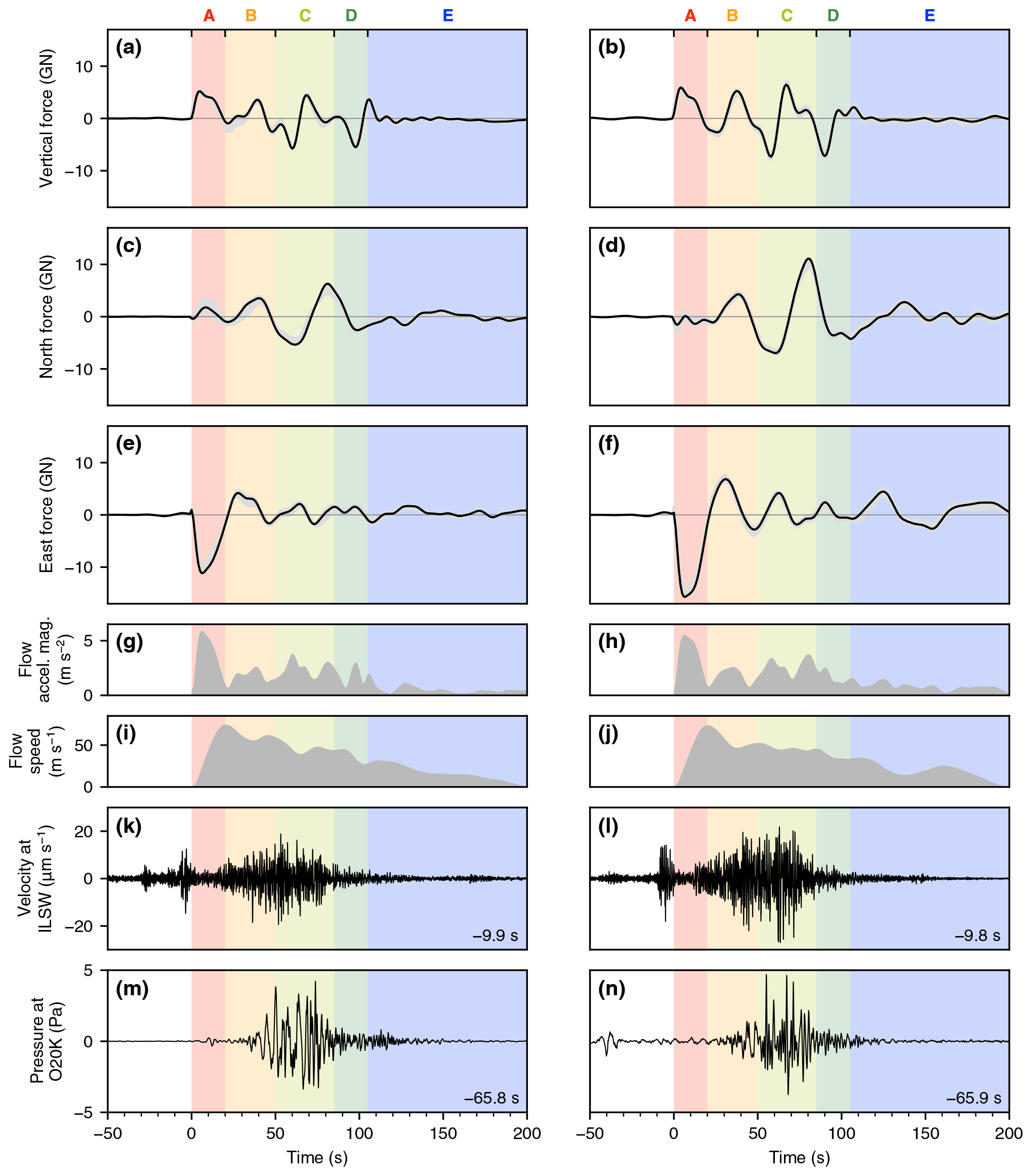
Figure 8 Force inversion results for the 2016 (left column) and 2019 (right column) events with seismoacoustic waveforms for reference. (a–f) Three-component (vertical, north, and east) force-time function f(t). Gray patches show the jackknife-derived minimum and maximum forces for f(t). (g, h) Force-derived center of mass (COM) acceleration magnitude $\Vert \mathit{a}\left(t\right)\Vert$. (i, j) Force-derived COM speed $\Vert \mathit{v}\left(t\right)\Vert$. (k, l) Vertical-component seismic waveforms from station ILSW shifted for travel time from the avalanche path midpoint using a Rayleigh group wave speed at 1 Hz of 900 m s⁻¹. (m, n) Infrasound waveforms from station O20K shifted for travel time from the avalanche path midpoint using an acoustic wave speed at 10 ^∘C of 337 m s⁻¹. The time shifts are indicated on the corresponding plots. Seismoacoustic waveforms are high-pass filtered at 0.1 Hz. The time axes are relative to the inversion zero time. Vertical axis scales are equal for each row. Colored patches correspond to those in Fig. 10 and the letters A–E in Sect. 6.2.

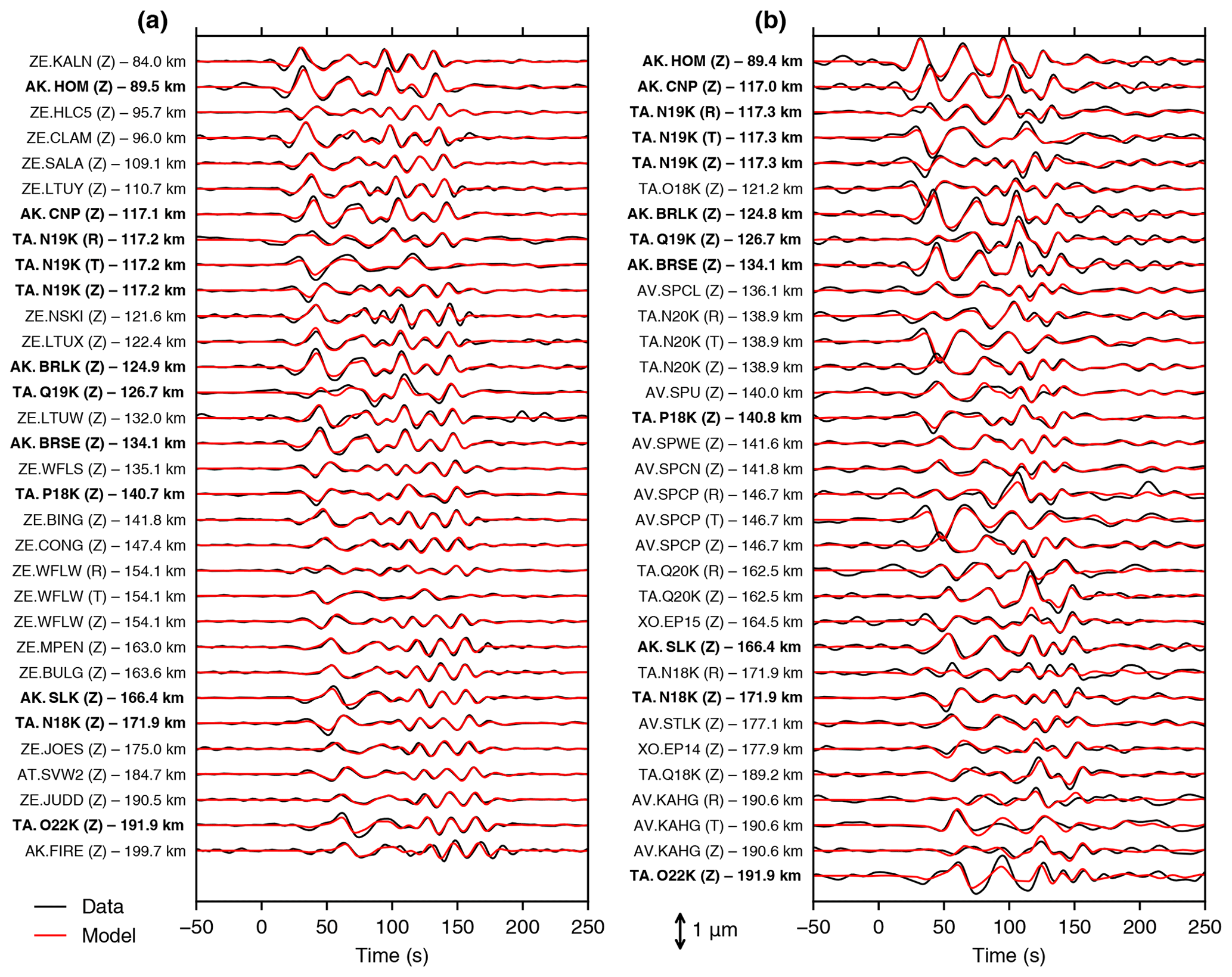
Figure 9 Waveform fits for the (a) 2016 and (b) 2019 force inversions. Observed data are plotted as black lines; modeled data are shown as red lines. Letters in parentheses indicate vertical (Z), radial (R), and transverse (T) components, and distance to the point force location is noted for each waveform. Boldface labels indicate components of stations used in both inversions (see Fig. 1). Waveforms are not individually normalized, and the amplitude scale is identical between (a) and (b). The time axes are relative to the inversion zero time. (See Sect. 3 for description of network codes.)

The avalanches initiate with an upward- and westward-directed force, indicating acceleration of the avalanche down and to the east. This is followed by a complicated yet strikingly similar “coda” for the two events. There are prominent northward force peaks at ∼ 40 and ∼ 80 s. The second is sharper and larger in amplitude than the first. There is also a broad southward force occurring after the first (broad) northward force peak with about the same amplitude, at approximately 65 s. For both avalanches, the vertical component of f(t) contains two distinct “stair steps” where the force shifts from upwards, to near-zero, to downwards; these initiate at about 40 and 70 s. Both events conclude with an impulsive vertical downward force occurring at about 95 s in 2016 and 90 s in 2019. After this point, the vertical component is nearly zero, while the horizontal components show low-amplitude, long-period undulations which are more pronounced in 2019.

5.2.2 Trajectories and flow speeds

Seismically derived avalanche trajectories generally agree with true trajectories for both events. Map and vertical profile views of the force inversion trajectories for the two events are shown in Fig. 10. As expected given the highly similar force-time functions, the shapes of the trajectories are very similar. The horizontal displacements indicate that the avalanche COMs moved almost due east before curving to the south, north, and south again. The vertical profiles in Fig. 10c and d show minor undulations on an otherwise fairly constant slope and are strictly decreasing as expected. The black lines are slices through the SfM DEM along the corresponding horizontal trajectory. The vertical 2016 trajectory (Fig. 10c) and horizontal 2019 trajectory (Fig. 10b) show notable deviations from the DEM and imagery observations – we explore causes for this in Sect. 6.5. Jackknifed trajectories, shown as translucent colored lines in Fig. 10, show about 1 km of spread on either side of the true location for the horizontal COM end point. For both events, the dominant eastward directionality is evident regardless of jackknife iteration. Note that the jackknifed trajectories primarily show uncertainties related to station coverage and data selection effects; other sources of trajectory uncertainties which also grow with time are not captured by the jackknife procedure and are discussed in Sect. 6.5.

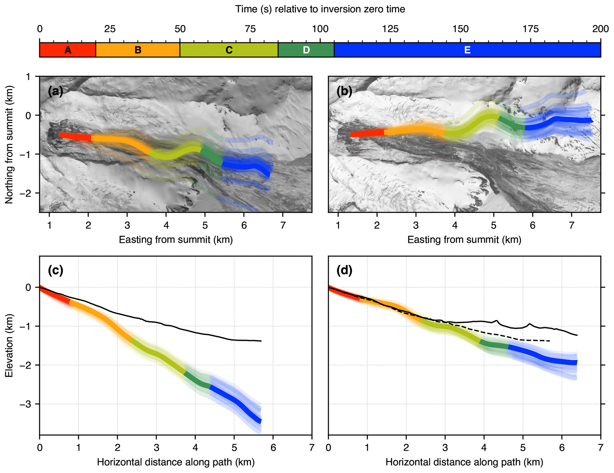
Figure 10 Map and profile views of trajectories integrated from the inversion force-time functions for the 2016 (a, c) and 2019 (b, d) events. Multiple translucent lines correspond to trajectories computed from the jackknife runs. Background images in (a) and (b) are the same as in Fig. 2. Black lines in (c) and (d) are profiles through the structure-from-motion digital elevation model (SfM DEM) along the corresponding horizontal trajectory. Dashed line in (d) is the SfM DEM profile from (c). Colored segments correspond to those in Fig. 8 and the letters A–E in Sect. 6.2. Imagery © 2016 and 2019 Planet Labs, Inc.

Force-inversion-derived COM runout distances and flow speeds have realistic magnitudes and are similar between the two events. Pinning the large northward force in f(t) to the flow lobe on the orographically downslope left side of the flow path as described in Sect. 4.3.3 gives a horizontal along-path COM distance L_COM of 5.7 km with a corresponding mass of 2.1×10⁹ kg for the 2016 event. For the 2019 event, L_COM=6.4 km and the mass is 3.0×10⁹ kg. Both trajectories indicate that most of the avalanche COM displacement occurred within the first ∼150 s of flow (Fig. 10). Average and maximum speeds obtained by integration of f(t) are 33 and 75 m s⁻¹ in 2016 and 34 and 74 m s⁻¹ in 2019, respectively. Note that these results are all derived from the force inversion magnitudes. Our satellite-imagery-derived calculations yield volumes of ($\mathrm{13}\pm \mathrm{8})\times {\mathrm{10}}^{\mathrm{6}}$ m³ in 2016 and ($\mathrm{11}\pm \mathrm{7})\times {\mathrm{10}}^{\mathrm{6}}$ m³ in 2019. The corresponding masses are ($\mathrm{22}\pm \mathrm{14})\times {\mathrm{10}}^{\mathrm{9}}$ kg in 2016 and ($\mathrm{19}\pm \mathrm{13})\times {\mathrm{10}}^{\mathrm{9}}$ kg in 2019.

6 Discussion

6.1 Acoustic source directionality

We lack sufficient infrasound station coverage to fully test an applicable acoustic source model, such as a single or distributed dipole, so we do not attempt an acoustic source inversion (e.g., Kim et al., 2012; Iezzi et al., 2019) here. Our infrasound analysis is, therefore, largely qualitative. By modeling infrasound propagation and site noise conditions, we sought to isolate source properties, such as size and directionality, from path effects. For example, Perttu et al. (2020) found that atmospheric propagation effects could not explain the infrasound radiation pattern observed for the 2018 Anak Krakatau flank collapse, and they used this to infer that the collapse acted like a piston, pushing sound in a directed manner.

For the Iliamna avalanches, examination of acoustic propagation alone might lead one to believe that source directionality is present, given the consistent detections of stations to the east of Iliamna despite variable local propagation conditions between the two events. However, there are two complicating factors in our case. First, station noise analysis (Fig. 6) shows that local stations to the west of Iliamna (and to the north and south as well in 2019) had high noise levels, indicating that preferential detection on stations to the east could simply be due to lower noise levels at those stations. Second, while rugged topography surrounds Iliamna, there is less topography blocking propagation to the east than to the west (Fig. 1). Furthermore, the avalanches occurred on the east flank of Iliamna. Because infrasound propagation at local distances is strongly controlled by topography (Kim et al., 2015), propagation to the east from Iliamna may be topographically preferred. These complicating factors preclude us from assessing source directionality or obtaining quantitative source estimates.

6.2 Multistage failure and flow

Synthesis of the force-time function with high-frequency waveforms and force-derived COM acceleration magnitudes and speeds (Fig. 8) as well as force-derived trajectories (Fig. 10) suggests a consistent multistage failure and flow pattern for both avalanches. Our interpretation is as follows, with approximate times relative to the inversion zero time as well as color codes given in brackets:

• A.

  The initial failure of the source region in ice or at the ice–bedrock interface occurs. Subsequent sliding at an average angle of ∼ 20–25^∘ begins, manifested as a high-frequency (> 5 Hz) seismic transient and a substantial eastward acceleration. No detectable infrasound is generated by the initial failure (the small pulse visible at ∼ 10 s in 2016 is not seen on any other stations or arrays and is, therefore, likely noise) [0–20 s; red].

• B.

  The avalanche mass reaches its maximum speed and material becomes fragmented, changing the flow regime from coherent to granular and turbulent. This is manifested as a gradual increase in the high-frequency (> 5 Hz) seismic energy; infrasound energy begins to rise simultaneously as the flow bends to the south [20–50 s; orange].

• C.

  The now fragmented flow bends to the north and then to the south as both high-frequency seismic and infrasound signals reach their peak amplitudes. Flow speeds decrease but stay between ∼ 30 and 60 m s⁻¹ [50–85 s; light green].

• D.

  The flow encounters a change to a shallower slope angle (< 10^∘) where a tributary glacier joins Red Glacier from the southwest (see Fig. 2). This is manifested as an impulsive, relatively short-period (∼ 30 s) downward force. The high-frequency seismic and infrasound signals taper off and flow speeds continue a slow decline [85–105 s; dark green].

• E.

  After passing the kink in topography where the slope angle decreases, the flow broadens and decelerates, forming the wide, flat debris lobe seen in Fig. 2. The east component of f(t) is largely positive, indicating deceleration of the flow. The vertical component of f(t) is near-zero, and this portion of the flow is not seismically or acoustically energetic for frequencies > 0.1 Hz [105+ s; blue].

Our trajectories are compatible with numerical flow models for Red Glacier avalanches performed by Huggel et al. (2007) and Schneider et al. (2010), which both indicate that the avalanche COM tends to the orographic downslope right and then downslope left, in the latter case forming a superelevation-like flow lobe visible in Fig. 2. We do not consider the possibility that the observed deposit was formed by two separate flows, as suggested by Huggel et al. (2007) for the 1980 and 2003 Red Glacier avalanches, because we do not see evidence for two separate flows in the seismoacoustic signals or in satellite imagery of the deposits (Fig. 2), and our modeling assuming a single flow is compatible with previous modeling and observations. This suggests that only one flow took place, at least in 2016 and 2019.

6.3 Mass estimation

One complication of extracting quantitative information from the force inversion results concerns the method of regularization. Because we impose penalties on the size, slope, and roughness of f(t) via the a_i coefficients (see Appendix A), the resultant force amplitudes are likely artificially depressed compared with the true values, as mentioned in Sect. 4.3.3. This is evidenced by the much smaller magnitude of the masses from the force inversion trajectories versus our satellite-imagery-based estimates (2.1 and 3.0 ×10⁹ kg versus 22 and 19 ×10⁹ kg for the 2016 and 2019 events, respectively). Even the lower bounds on our imagery-based mass estimates are still far larger than their inversion-derived equivalents, suggesting that the force amplitudes are indeed being suppressed by the regularization scheme (see Appendix A). Additionally, we are inverting a band-limited signal – energy present at very long periods (> 80 s) is not reflected in f(t), which also artificially depresses f(t). Due to these biases, we do not apply the scaling relationship of Ekström and Stark (2013) to these results. We note that in general the masses of these events are not well constrained due to poor constraints on deposit thickness and the relative contributions of entrainment and deposition to the total failure mass. Better ground observations of avalanche deposit properties would help constrain the effect of regularization, and we encourage such studies in the future. We do note that the phase and relative amplitude of the force-time functions between the two events (Fig. 8a–f) are not affected by the regularization.

6.4 Flow dynamics

Average flow speeds for mass movements can be estimated from the duration of the high-frequency seismic envelope if the horizontal runout length L is known (Caplan-Auerbach et al., 2004). However, it is often difficult to estimate the duration of the flow from the seismic envelope, because the noise floor can bury the earliest and latest parts of the emergent signal (Huggel et al., 2007). Caplan-Auerbach and Huggel (2007) estimated average flow speeds of about 20–50 m s⁻¹ for Red Glacier avalanches using this method. A more complete assessment of flow speeds can be obtained from numerical modeling or by examination of the speed time series $\Vert \mathit{v}\left(t\right)\Vert$ obtained from the force inversion, as these provide both average and maximum values. Schneider et al. (2010) found an average flow speed of about 50 m s⁻¹ and peak flow speeds between 70 and 100 m s⁻¹ for a numerically modeled 2003 Red Glacier avalanche. Our values derived from $\Vert \mathit{v}\left(t\right)\Vert$ (average speeds of 33 and 34 m s⁻¹ and maximum speeds of 75 and 74 m s⁻¹ in 2016 and 2019, respectively) are compatible with these results as well as those of Caplan-Auerbach and Huggel (2007), although we note that our values describe COM dynamics, whereas those of Caplan-Auerbach and Huggel (2007) are calculated using L and, therefore, apply to the flow front. Our results are also broadly compatible with other studies of similar large avalanches, such as the July 2007 Mount Steele rock–ice avalanche (35–65 m s⁻¹ average speed; Lipovsky et al., 2008) and the June 2016 Lamplugh Glacier rock avalanche (∼55 m s⁻¹ maximum speed; Dufresne et al., 2019).

Inversion-derived COM acceleration magnitudes $\Vert \mathit{a}\left(t\right)\Vert$ and flow speeds $\Vert \mathit{v}\left(t\right)\Vert$ are plotted in Fig. 8g–j. The peak infrasound amplitude does not correlate with the peak acceleration magnitude nor the peak speed, instead occurring about 50 s after the latter. This notable latency between peak speed and peak acoustic energy might be explained by a model similar to Marchetti et al. (2019), where infrasound is produced by waves at the free surface of the flow. Such waves would take time to develop because the initially blocky mass needs to be sufficiently fragmented and turbulent, which requires high flow speeds. The infrasound and seismic waveforms (Fig. 8k–n) do exhibit similar shapes and reach their peak values at approximately the same time (after travel time removal). This alignment of high-frequency seismic and infrasound signals has previously been observed for debris flows (Schimmel et al., 2018; Marchetti et al., 2019) and suggests that after some initial breakup period, Iliamna ice–rock avalanches may exhibit similar flow dynamics to debris flows, at least seismoacoustically.

Another possibility is that flow interaction with a particular topographic feature along the flow path is generating infrasound and that the observed peak amplitude timing corresponds to the time for the flow to reach this feature. Figure 8m and n indicate that peak infrasound occurs anywhere from 50 to 85 s into the flow. Because the prominent northward force linked to the flow lobe on the orographically downslope left side of the flow occurs at about 80 s, flow turbulence at this point could be responsible for the peak in infrasound energy. Moore et al. (2017) observed a ground-coupled airwave associated with the second of two very large rock avalanches at Bingham Canyon Mine (Utah, USA). They inferred from the timing of the phase that the airwave was likely coupled into the ground when the rock avalanche was beginning to impact the pit bottom, ∼50 s after the start of the event. However, this explanation makes less sense in the context of the Red Glacier avalanches because the topography of Red Glacier is far smoother (e.g., compare the black line in Fig. 10c to Fig. 5 in Moore et al., 2017).

6.5 Inversion stability and trajectory uncertainties

The low variance of the jackknife iterations (Fig. 8a–f) indicates that the inversion result is largely unaffected by changes to the input data. However, we note two prominent issues with the calculated trajectories:

1. The 2019 horizontal trajectory is rotated approximately 15^∘ counterclockwise relative to the 2016 trajectory, although both have the same shape.

2. The 2016 vertical trajectory is too steep relative to the bed topography (black line in Fig. 10a).

There are several potential causes for these discrepancies. One possibility is that our model loses validity over the course of the event. Because the premise of the force inversion assumes a single point force, as the avalanche moves downslope and transitions from a sliding block to a more distributed, fragmented flow, our source model becomes less applicable (see Coe et al., 2016). However, the horizontal trajectories provide a reasonable quantitative estimate for the entire flow path, not just the initial period of supposed higher model validity. Ultimately, without video footage of the events, improved mass estimates, or sophisticated flow modeling, understanding where the model may begin to break down is challenging.

Another factor is noise within the passband of our inversion. We note that while the SNR for the longer-period portion of the inversion passband was generally greater in 2019 than in 2016, the SNR for shorter periods (15–25 s) was lower in 2019 than in 2016 (Fig. 5). This greater short-period noise in 2019 is visible when comparing the waveforms in 2016 (Fig. 9a) to those in 2019 (Fig. 9b). We were unable to avoid this noise without increasing the minimum period of the inversion and, therefore, sacrificing short-period details in f(t), which are consistent between the two events and, thus, not spurious. As this short-period noise is more prominent in 2019 than 2016, it could contribute to the misaligned horizontal trajectory for the 2019 event. We note that the variance reduction (VR) for the 2019 inversion is about 10 % lower than the VR for the 2016 inversion; this is readily seen in Fig. 9.

Finally, our inversion may be biased by uneven azimuthal station coverage or an uneven distribution of seismometer components. For most stations, horizontal components tended to be noisier than vertical components. Consequently, most of our input waveform data for the inversion is vertical component (see component labels in Fig. 9). Mathematically, Eq. (1) shows that given sufficient azimuthal coverage, f(t) should be recoverable from the vertical displacement time series u_Z(t) alone. However, our largely vertical-component input data could be causing our f_Z(t) amplitudes to be biased too high. This, in turn, would produce overly steep vertical trajectories. We tested the inversion's sensitivity to azimuthal station coverage and found that the 2019 trajectory showed negligible change unless significant deviations (e.g., only retaining stations to the south of Iliamna) were undertaken.

All of the preceding issues are exacerbated when we doubly integrate f(t) to obtain displacement. Therefore, a relatively small southward bias in f(t) could nudge the entire trajectory northward in the manner seen for the 2019 event. This also applies to the overly steep vertical trajectory in 2016 – if at any point in f(t) the vertical component is overestimated, the vertical trajectory will be affected from that point onwards. In spite of these issues, the consistent shape of the trajectories and the strikingly similar phase and relative amplitude of the force-time functions give us confidence in our modeling.

6.6 Comparing events

A key benefit of modeling two highly similar avalanches is the opportunity to compare the inversion results, determine which features are consistent between the two events, and evaluate the inversion technique. Examination of f(t) for the 2016 event alone might lead one to conclude that the shorter-period details are just spurious byproducts of noise or path effects. However, the 2019 avalanche has flow and deposit characteristics that are remarkably similar to those of the 2016 event, and we observe similar details in f(t) in spite of varying path effects due to different station configurations in 2016 and 2019. This provides more confidence in the inversion method used here.

One notable difference between the force-time functions obtained for the two avalanches is the increased amplitude for the 2019 event. This increase is consistent across all three force components, yet it is unlikely to be an inversion artifact because both inversions have the same regularization parameters. The high-frequency seismic signals (Fig. 8k, l) also indicate larger amplitudes for the 2019 event. Because the observed deposits have similar sizes (see Fig. 2), this suggests that a larger amount of mass was moved in 2019 than in 2016 but with little change in runout length. The mass discrepancy could be caused by varying initial failure thicknesses (i.e., a thicker crown in 2019) or an increased portion of rock involved in the 2019 event versus the 2016 event. Unfortunately, we do not possess the field-based observations and measurements necessary to test these hypotheses.

6.7 Feasibility for rapid hazard response

The detailed information on avalanche dynamics retrievable from the rapidly recorded seismic signals for these events raises the question of the suitability of this method for near-real-time applications. Besides the seismic signals themselves, only two independent pieces of information are required to obtain 3D trajectories: the event location (for locating the point force) and the failure mass (for converting force to acceleration). In this study, we used high-resolution satellite imagery to estimate the former.

In the absence of any independent data, the following could be performed: the event location could be estimated using traditional earthquake or mass-movement-specific location methods (see Allstadt et al., 2018, and references therein), and the failure mass could be roughly estimated from the scaling laws of Ekström and Stark (2013). A location could also be determined from infrasound signals using back projection (see, e.g., Sanderson et al., 2020). Note that due to the long wavelengths of the signals used, a precise location is not critical for the inversion process. The resulting seismically derived trajectory would be a rough approximation due to uncertainties in mass estimation and/or location. However, the directionality and relative size of the mass movement would be preserved, and this information could be harnessed to remotely determine the likely path and scale of a mass movement.

Unfortunately, automatic locations are not available for the two Iliamna events or other events of comparable size. However, we note that the very large June 2016 Lamplugh Glacier, Alaska, rock avalanche (see Bessette-Kirton et al., 2018; Dufresne et al., 2019) has a cataloged location and origin time. In general, at this time an automatic inversion method would likely be successful only for very large mass movements with high SNR seismic and acoustic waveforms. We note that our methods are primarily aimed at providing information complementary to other techniques; they do not currently constitute a stand-alone or automated technique. Still, in remote settings where event information from other sources may be delayed or unavailable – such as Alaska – this approach could provide key estimates of basic flow properties in near-real time.

7 Conclusions

Surficial mass movements transfer energy into the solid Earth and the atmosphere, producing seismoacoustic signals that yield complementary information about event dynamics. In this study, we analyze an exceptional seismoacoustic dataset from two large, highly similar ice–rock avalanches to reconstruct the dynamics of the events. The similarity of these avalanches provides an excellent opportunity to test the robustness of our modeling methods. Our force-time functions are derived from the inversion of long-period (15–80 s) seismic signals recorded on stations > 80 km from the avalanches. They indicate that over the course of about 150 s, the avalanche COM slid to the east, was subsequently deflected slightly to the south and then to the north, and then broadly decelerated. Our results provide constraints on time-varying avalanche acceleration, velocity, and directionality. This is important for hazard mitigation as well as general understanding of seismic signals from mass movements, although better estimates of mass and flow properties from field studies (e.g., Dufresne et al., 2019) and numerical modeling (e.g., Moretti et al., 2012) are needed to fully exploit this method's potential.

While it was possible to model the avalanche seismic source, we lacked sufficient infrasound data to quantitatively characterize the acoustic source. After accounting for propagation effects and station noise, we cannot assess whether the Iliamna avalanches exhibit acoustic source directionality. Still, the acoustic data are qualitatively consistent with our force-derived reconstructions. It appears that infrasound from these avalanches is produced after the mass movement regime transitions from cohesive block-type failure to granular and turbulent flow, but controlled experiments and denser acoustic instrumentation are needed to fully test this hypothesis.

Iliamna Volcano is an excellent site for the seismoacoustic and geomorphological study of these impressive avalanches due to their relatively frequent occurrence at the volcano. Future work at Iliamna – as well as at other sites of repetitive surficial mass movements – should synthesize advanced numerical modeling techniques with detailed observations including video footage and repeat high-resolution DEM acquisitions. These efforts, combined with more complete acoustic station coverage – perhaps with arrays as well as single sensors – could result in a substantial increase in our understanding of the behavior of large debris avalanches and other mass movements. This insight may then be applicable for mitigation of, and response to, the significant hazards posed by these dramatic surface processes.

Appendix A: Inversion formulation and constraints

Consider the convolutions given by Eqs. (1)–(3). In numerical contexts, it is more convenient to formulate these convolutions as matrix multiplications. Therefore, we transform the Green's functions (GFs) into convolution matrices Λ by reversing the GFs in time and staggering them as in Allstadt (2013), where the time dependence of the GF is now implicitly stored in the matrix. (For example, the multiplication Λ_ZVf_Z corresponds to the convolution f_Z(t)*g_ZV(t); see Eq. A5 in Allstadt, 2013) Making this modification, we can combine Eqs. 1–3 (dropping the explicit time dependence for brevity) into

$$\begin{array}{}\text{(A1)}& {\mathit{u}}^k={\mathbf{\Gamma }}^k\mathit{f},\end{array}$$

where now the superscript k denotes the station and Γ^k is a matrix of GF convolution matrices:

$$\begin{array}{}\text{(A2)}& {\mathbf{\Gamma }}^k=\left[\begin{array}{ccc}{\mathbf{\Lambda }}_{\mathrm{ZV}}^k& {\mathbf{\Lambda }}_{\mathrm{ZH}}^k\cos {\mathit{\varphi }}^k& {\mathbf{\Lambda }}_{\mathrm{ZH}}^k\sin {\mathit{\varphi }}^k\\ {\mathbf{\Lambda }}_{\mathrm{RV}}^k& {\mathbf{\Lambda }}_{\mathrm{RH}}^k\cos {\mathit{\varphi }}^k& {\mathbf{\Lambda }}_{\mathrm{RH}}^k\sin {\mathit{\varphi }}^k\\ \mathbf{0}& {\mathbf{\Lambda }}_{\mathrm{TH}}^k\sin {\mathit{\varphi }}^k& -{\mathbf{\Lambda }}_{\mathrm{TH}}^k\cos {\mathit{\varphi }}^k\end{array}\right].\end{array}$$

We can now write the linear forward model for N stations as

$$\begin{array}{}\text{(A3)}& \mathit{d}=\mathbf{G}\mathit{f},\end{array}$$

with $\mathit{d}={\left[{\mathit{u}}^{\mathrm{1}},{\mathit{u}}^{\mathrm{2}},\mathrm{\dots },{\mathit{u}}^k,\mathrm{\dots },{\mathit{u}}^N\right]}^{\top }$ and $\mathbf{G}={\left[{\mathbf{\Gamma }}^{\mathrm{1}},{\mathbf{\Gamma }}^{\mathrm{2}},\mathrm{\dots },{\mathbf{\Gamma }}^k,\mathrm{\dots },{\mathbf{\Gamma }}^N\right]}^{\top }$. The superscript ⊤ denotes the transpose; d is a 1D column vector consisting of the data predicted for each component of each station u^k concatenated end-to-end. This is an ill-conditioned problem, so regularization is required to reduce the condition number of G. We invert for f using a higher-order Tikhonov-regularized least squares formulation (e.g., Aster et al., 2013). The solution is

$$\begin{array}{}\text{(A4)}& \mathit{f}={\left[{\mathbf{G}}^{\top }\mathbf{G}+{\mathit{\alpha }}^{\mathrm{2}}\left(a_{\mathrm{0}}\mathbf{I}+a_{\mathrm{1}}{{\mathbf{L}}_{\mathrm{1}}}^{\top }{\mathbf{L}}_{\mathrm{1}}+a_{\mathrm{2}}{{\mathbf{L}}_{\mathrm{2}}}^{\top }{\mathbf{L}}_{\mathrm{2}}\right)\right]}^{-\mathrm{1}}{\mathbf{G}}^{\top }\mathit{d},\end{array}$$

where I is the identity matrix, and L₁ and L₂ are first- and second-order roughening matrices which approximate the first and second derivatives, respectively. The coefficients a₀, a₁, and a₂ control the degree of importance given to “small,” “flat,” and “smooth” models, respectively. They must sum to one:

$$\begin{array}{}\text{(A5)}& \sum _{i=\mathrm{0}}^{\mathrm{2}}{a}_i=\mathrm{1}.\end{array}$$

The regularization parameter α is chosen to balance the constraints on the model specified by the a_i coefficients while still fitting the data well. We use the L-curve criterion (Hansen, 1992) to find the optimal value for α. For both inversions, we found the optimal values for these parameters were $\mathit{\alpha }=\mathrm{5.3}\times {\mathrm{10}}^{-\mathrm{17}}$ and $a_i=[\mathrm{0.4},\mathrm{0},\mathrm{0.6}]$. This selection of a_i parameters prioritizes a model that is both small in magnitude (more centered on zero) and smooth. The inclusion of the higher-order regularization matrices L₁ and L₂ in Eq. A4 separates this method from the method used in Allstadt (2013) and Coe et al. (2016), which only included zeroth-order Tikhonov regularization.

To characterize the fit of the model to the data, we compute the variance reduction (VR), which is defined as

$$\begin{array}{}\text{(A6)}& \mathrm{VR}=\left(\mathrm{1}-{\displaystyle \frac{\Vert \mathit{d}-{\mathit{d}}_{\mathrm{obs}}{\Vert }^{\mathrm{2}}}{\Vert {\mathit{d}}_{\mathrm{obs}}{\Vert }^{\mathrm{2}}}}\right)\times \mathrm{100}\mathit{\%},\end{array}$$

where d_obs are the observed data and d are the synthetic data predicted by the forward model (Eq. A3).

In addition to regularization, we constrain all of the components of f to sum to zero to conserve the total momentum of the Earth (see Appendix A in Allstadt, 2013). We also enforce all components of f be zero prior to a specified “zero time.” We choose the zero time to correspond to the point where the vertical component f_Z(t) is non-zero and rising, signaling the initial downward acceleration of the avalanche. The zero time for the 22 May 2016 event is 07:57:57, and the zero time for the 21 June 2019 event is 00:03:13. The selection of the zero time was unambiguous for both events.

To assess the stability of the inversion, we use a variation on the jackknife technique (e.g., Moretti et al., 2015; Coe et al., 2016). We run 20 iterations of the inversion, each time randomly discarding 30 % of the waveforms.