the Creative Commons Attribution 4.0 License.
the Creative Commons Attribution 4.0 License.
 | 04 Feb 2021
Coupling threshold theory and satellite-derived channel width to estimate the formative discharge of Himalayan foreland rivers
Kumar Gaurav
François Métivier
A V Sreejith
Rajiv Sinha
Amit Kumar
Sampat Kumar Tandon
We propose an innovative methodology to estimate the formative discharge of alluvial rivers from remote sensing images. This procedure involves automatic extraction of the width of a channel from Landsat Thematic Mapper, Landsat 8, and Sentinel-1 satellite images. We translate the channel width extracted from satellite images to discharge using a width–discharge regime curve established previously by us for the Himalayan rivers. This regime curve is based on the threshold theory, a simple physical force balance that explains the first-order geometry of alluvial channels. Using this procedure, we estimate the formative discharge of six major rivers of the Himalayan foreland: the Brahmaputra, Chenab, Ganga, Indus, Kosi, and Teesta rivers. Except highly regulated rivers (Indus and Chenab), our estimates of the discharge from satellite images can be compared with the mean annual discharge obtained from historical records of gauging stations. We have shown that this procedure applies both to braided and single-thread rivers over a large territory. Furthermore, our methodology to estimate discharge from remote sensing images does not rely on continuous ground calibration.
- Article
(16960 KB) - Full-text XML
- BibTeX
- EndNote


The measurement of river discharge is necessary to investigate channel morphology, sediment transport, flood risks, and to assess water resources. Despite this, the discharge of many rivers remains unknown, especially those located in sparsely populated regions, at high latitudes, or in developing countries. Even now, the discharge is measured at sparsely located stations along a river's course (Smith and Pavelsky, 2008; Andreadis et al., 2007). Between measurement stations, the discharge is interpolated using routine techniques (Smith and Pavelsky, 2008). Furthermore, these local measurement stations are installed where the river flows as a single-thread channel and has a stable boundary. This is often not the case for braided rivers, where the flow is distributed through multiple and mobile threads (Smith et al., 1996; Ashmore and Sauks, 2006). Therefore, braided rivers are often not gauged; when this does occur, the gauging stations are located in places like dams with artificially regulated flow. This hinders our ability to assess discharge in the individual threads of a braided river.
To overcome this problem, as well as to minimise the costs related to discharge measurement, methodologies have been developed to use remotely sensed images to estimate the instantaneous discharge of rivers (Smith et al., 1996; Smith, 1997; Alsdorf et al., 2000, 2007; Ashmore and Sauks, 2006; Marcus and Fonstad, 2008; Papa et al., 2010, 2012; Gleason and Smith, 2014; Durand et al., 2016; Gleason et al., 2018; Allen and Pavelsky, 2018; Moramarco et al., 2019; Kebede et al., 2020). These studies establish rating relationships between some image-derived parameters (width and water level or stage and slope) and the instantaneous discharge measured in the field (Leopold and Maddock, 1953). Equations that define the hydraulic geometry of a channel relate the width (W), average depth (H), and slope (S) of a channel to the bankfull discharge (Q) according to
where a, b, c, e, f, and g are site-specific constants and exponents. Therefore, the available methods (based on remote sensing data) to estimate the discharge of a river cannot be extrapolated to other rivers or even to other locations on the same river. Moreover, as these rating curves vary significantly between locations, they must be established for each location independently. For example, Smith et al. (1995), Smith (1997), Smith and Pavelsky (2008), and Ashmore and Sauks (2006) used synthetic aperture radar and ortho-rectified aerial images to estimate discharge in braided rivers. They related the image-derived effective width of a braided river to the discharge at a nearby gauging station to establish a relationship in the form of Eqs. (1)–(3). Their approach provides an estimate of the total discharge in a braided river, at a given section. However, this technique is site-specific and assumes that the riverbed does not change over time.
Few attempts have been made to overcome these limitations; for example, Bjerklie et al. (2005) used aerial orthophotographs and synthetic aperture radar (SAR) images to estimate discharge in various single-thread and braided rivers. To estimate the discharge, they extracted the maximum water width at a given river reach. They then combined the image-derived channel widths with channel slopes obtained from topographic maps and a statistical hydrologic model. They reported standard errors of 50 %–100 %. However, after using a calibration function based on field observation, the error decreased to values as low as 10 %. Later, Sun et al. (2010) used Japan Earth Resource Satellite-1 (JERS-1) SAR images to measure the effective width of the Mekong River at the Pakse gauging station in Laos. They used a rainfall–runoff model to estimate the discharge from the image-derived width and suggested that, using this procedure, the discharge could be estimated in any ungauged river basin within an acceptable level of accuracy. They established a close agreement between the measured discharge of the Mekong River at Pakse station and the model estimate to the 90 % uncertainty level. As discussed earlier by Bjerklie et al. (2005), Sun et al. (2010) subsequently indicated that the precision can be improved by calibrating the rainfall–runoff model with a hydraulic geometry relation and that a calibrated rainfall–runoff model can be used to estimate the discharge in any ungauged river using the measured width only. Gleason and Smith (2014) have suggested that the discharge of a single-thread river can be estimated from satellite images only, without any ground measurements. They plotted the exponents and coefficients of hydraulic regime equations established at 88 different gauging stations along six rivers in the US and found that the exponents and coefficients are correlated. Recently, Kebede et al. (2020) used Landsat images to estimate daily discharge of the Lhasa River in the Tibetan Plateau. They utilised image-derived hydraulic variables to compute the discharge using a modified Manning equation and rating curves established from the in situ measurement of width and discharge.
The studies discussed above attempt to address the issue of site-specificity, and they propose methods to estimate discharge without empirical calibration. However Bjerklie et al. (2005), and Sun et al. (2010) also show that a better accuracy in discharge prediction can only be achieved with some calibration to ground measurements. Therefore, a physically robust method to resolve the site-specificity of rating curves remains to be described.
To address this issue of site-specificity, we have developed a semi-empirical width–discharge regime relation based on the threshold theory and field measurement of various braided and meandering rivers on the Ganga and Brahmaputra plains (Seizilles et al., 2013; Métivier et al., 2016; Gaurav et al., 2017). According to this relation, threads of braided and meandering rivers share a common width–discharge regime relationship. Therefore, we hypothesise that this regime equation can be used to estimate the first-order discharge of any river (braided or meandering) flowing on the Ganga and Brahmaputra plains (and perhaps on the entire Himalayan foreland) if the wetted width of the river channels is known. This study can also be used for various applications such as (i) monitoring the downstream evolution of discharge, (ii) filling the data gap between the gauging stations separated over a long distance, (iii) constructing the time series and trend analysis of discharge variation, and (iv) identifying the critical reaches in rivers that are under stress due to excessive extraction of water for agriculture, industrial, or domestic supply.
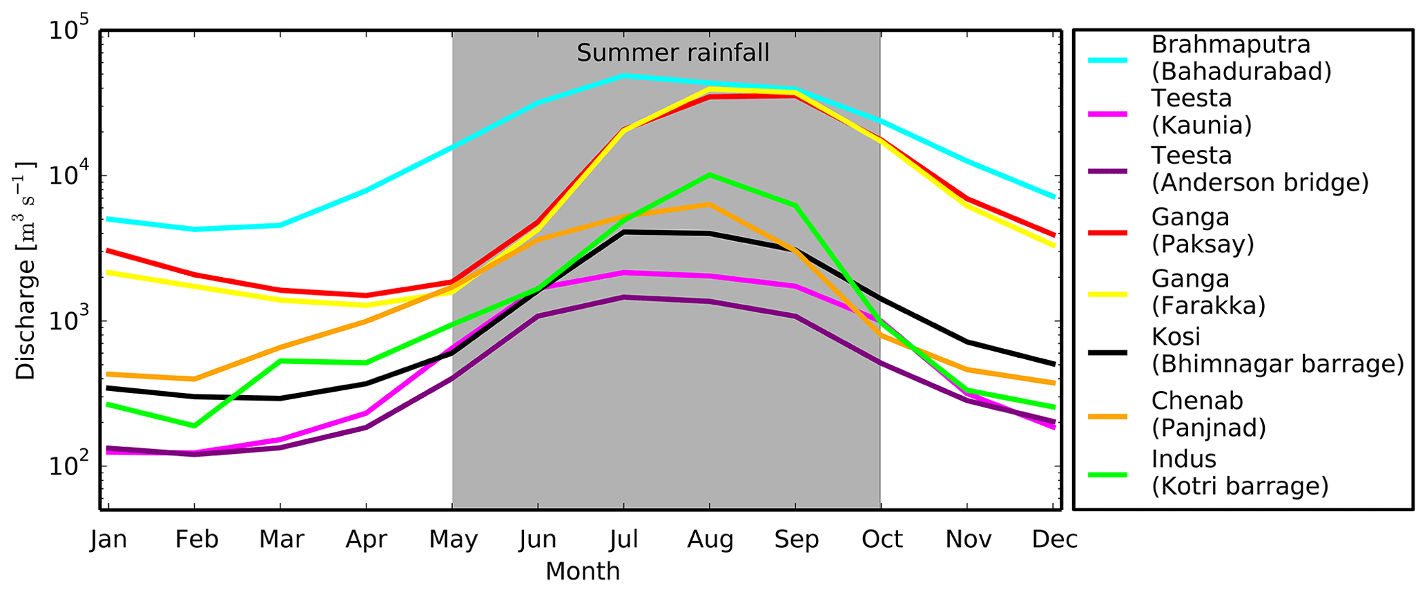
Many rivers flowing on the Indus–Ganga–Brahmaputra alluvial plains are perennial and have their source in the Himalayas and Tibetan Plateau. Flow of these rivers is primarily determined by snowmelt and rainfall during the Indian summer monsoon (Singh and Jain, 2002; Thayyen and Gergan, 2010; Bookhagen and Burbank, 2010; Andermann et al., 2012; Khan et al., 2017). However, the contribution of rainfall and snowmelt to the discharge of the Himalayan rivers can vary significantly along the orogenic strike. For example, on an annual timescale, snowmelt contributes about 15 %–60 % of discharge in the western Himalayan rivers, whereas it is less than 20 % in the eastern Himalayan rivers (Bookhagen and Burbank, 2010). These rivers experience a strong seasonal variability in their discharge – for instance, rainfall during the Indian summer monsoon (June–September) constitutes about 60 %–85 % of the annual discharge of the eastern Himalayan catchments and about 50 % of the annual discharge of the western Himalayan catchments.
A closer look into the hydrographs of the Himalayan rivers reveals two distinct flow regimes (Fig. 1): a clear separation of discharge during the summer monsoon and the rest of the period can be observed. From May to October, most of the Himalayan rivers flow at their peak discharge due to intense and prolonged rainfall and glacier melt in the catchment; in contrast, in the lean period (November–April), they carry relatively less discharge.
Lacey (1930) was the first to observe a dependency of the width of an alluvial river on its discharge. Based on measurements in various single-thread alluvial rivers and canals in India and Egypt, Lacey (1930) found that the width of a regime channel scales as the square root to the discharge (e∼0.5 in Eq. 1).
To explore the physical basis of the above-mentioned observation, Glover and Florey (1951) and Henderson (1963) developed a theory based on the concept of a threshold channel. According to this theory, with a constant water discharge, the balance between gravity and fluid friction maintains the sediment at a threshold of motion, everywhere on the bed surface. This mechanism sets the cross-section shape and size of a channel. The resulting W–Qw (width–discharge) relationship in dimensionless form reads as follows (Gaurav et al., 2014, 2017; Métivier et al., 2016, 2017):
where is the dimensionless water discharge, ds is the grain size, is the density of water, is the density of quartz, is the acceleration of gravity, Cf≈0.1 is the Chézy friction factor, μ≈0.7 is the Coulomb coefficient of friction, is the elliptic integral of the first kind, and θt is the threshold Shields parameter that depends on the sediments grain size. The typical grain size of the sediments of the Himalayan foreland rivers is of the order of ds=100–300 µm. Thus, the dimensionless grain size –6, where is the dynamic viscosity of water. In this range of values, the threshold Shields number is on order of θt∼0.1 with a maximum around 0.3 (Julien, 1995; Selim Yalin, 1992). Recently, Delorme et al. (2017) obtained an experimental value of θt∼0.25 for silica sands with a size of 150 µm. Here, we have taken the upper value of θt=0.3 as a conservative estimate. Taking lower values of the threshold Shields parameter, such as the classical 0.1, would lead to a slightly better match between the theoretical prediction and the data, but it does not lead to a significant change in our conclusions.
Equation (4) is the theoretical equivalent to Lacey's law. This theory explains the mechanism of how single-thread alluvial rivers, at threshold of sediment transport, adjust their geometry in response to the imposed water discharge. Strictly speaking, the mean equilibrium geometry of a natural alluvial channel is not set by a single discharge; rather, a range of discharges are responsible for determining the channel form (Leopold and Maddock, 1953; Wolman and Miller, 1960; Blom et al., 2017; Dunne and Jerolmack, 2020). However, the value that corresponds to the channel-forming discharge of an alluvial river remains a matter of debate. Wolman and Miller (1960); Wolman and Leopold (1957); Phillips and Jerolmack (2016) proposed that the bankfull discharge and discharge associated with a certain frequency distribution can be used to define the channel-forming discharge.
As threshold theory predicts the scaling relationship of a single-thread channel, one may consider applying it to assess the discharge that relates to the present-day geometry of natural alluvial channels. To test this, we use the regime curve that we established from threshold theory and the measurement of hydraulic geometry of various sandy alluvial rivers in the Himalayan foreland (Gaurav et al., 2014, 2017). In field campaigns during 2012, 2013, 2014, and 2018, we measured the geometry (width, depth, velocity, and median grain size) of individual threads of braided and meandering rivers spanning the Ganga and Brahmaputra plains. To measure the channel geometry, we used an acoustic Doppler current profiler (ADCP) on an inflatable motor boat. Close to the location of our ADCP-measured transects, we collected a sediment sample from the channel. We sieved the sediment sample in the laboratory to calculate the median grain size (d50). Detailed descriptions of the measurement can be found in our previous publications (Gaurav et al., 2014, 2017).
Figure 2 suggests that the individual threads of the Himalayan foreland rivers share a common width–discharge regime relation, and their morphology can be explained by threshold theory to the first order. The theoretical exponent accords with the empirical exponent of the width–discharge curve. However, the threads are wider than predicted by a factor of about 2 (Fig. 2). We now adjust the prefactor predicted from threshold theory to our data while retaining the theoretical exponent to establish a generalised semi-empirical “width–discharge” regime relationship for the Himalayan foreland rivers (Fig. 2). We then use this curve to estimate the discharge of various rivers of the Himalayan foreland by measuring their width from satellite images.

Figure 2Dimensionless width of the individual threads of the Himalayan foreland rivers as a function of dimensionless water discharge (following Gaurav et al., 2017). These data (width, discharge, and grain size) were acquired during the different field campaigns in the years 2012, 2013, 2014, and 2018. The measurements were performed during the period when the Himalayan rivers usually flow at their formative discharge. The solid line (dark) is the prediction from threshold theory, and the solid line (light) is obtained by fitting the prefactor of the threshold relation (Eq. 4) to the data while retaining the theoretical exponent.
4.1 Dataset
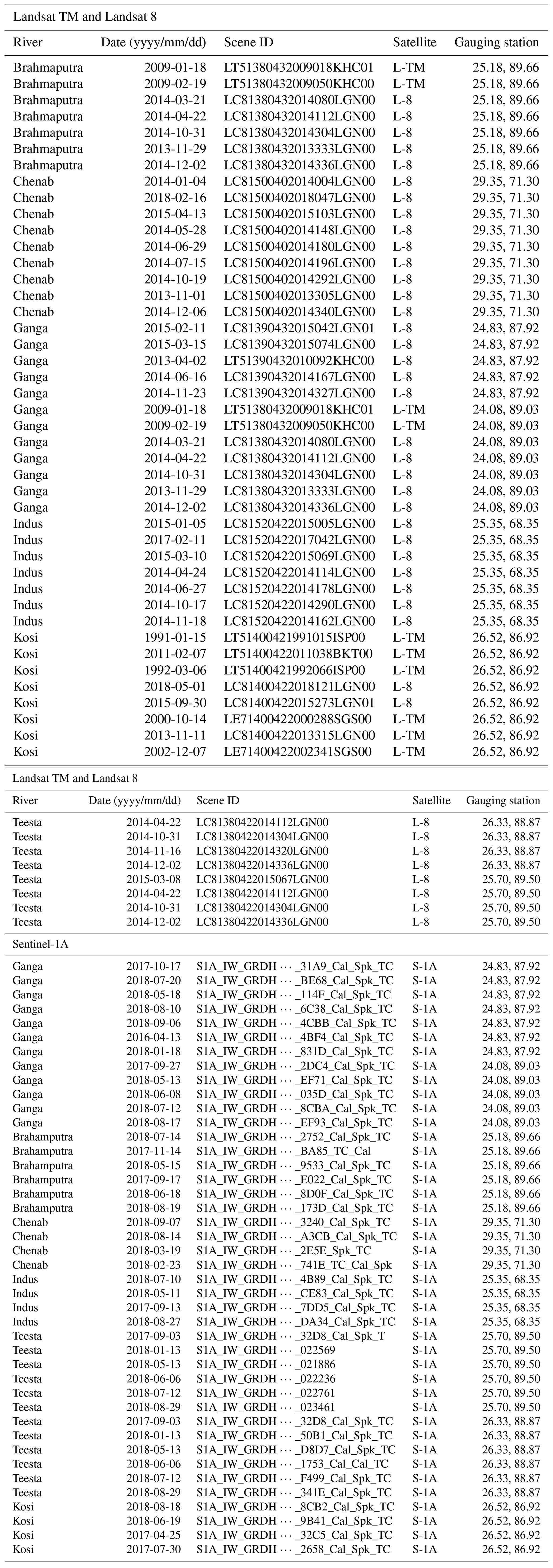
To measure the width of a river channel, we use images acquired from Landsat Thematic Mapper (TM), Landsat 8, and Sentinel-1A satellites (Appendix A1). All images of the Landsat and Sentinel satellite missions are freely available, and they can be downloaded from the US Geological Survey (https://earthexplorer.usgs.gov, last access: 7 March 2019) and Alaska Satellite Facility (https://www.asf.alaska.edu/sentinel, last access: 7 March 2019) websites. We downloaded all available cloud-free Landsat satellite images at the locations that were near the in situ measurement stations for which discharge data were available to us (Fig. 3). Only a few cloud-free Landsat images are available for the period from June to September. This is mainly because of the strong monsoon that causes intense rainfall and dense cloud cover. To overcome seasonal effect and fill the data gap during the monsoon period, we use the Sentinel-1A product. The Sentinel-1 satellite mission is equipped with an advanced synthetic aperture radar (ASAR) sensor that operates in the C-band (5.4 GHz) of microwave frequency (Schlaffer et al., 2015; Martinis et al., 2018). The advanced synthetic aperture radar system can operate both day and night and has the capability to penetrate clouds and heavy rainfall. This special characteristic of SAR sensors also enables uninterrupted imaging of the Earth's surface during bad weather conditions.
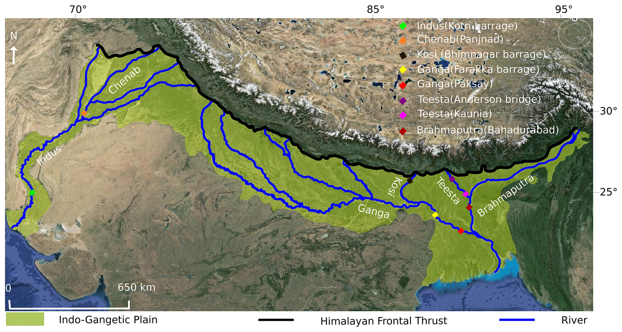
Figure 3Locations of the gauging stations of various rivers in the Indus, Ganga, and Brahmaputra basins for which discharge data are available (source: © Google Earth).
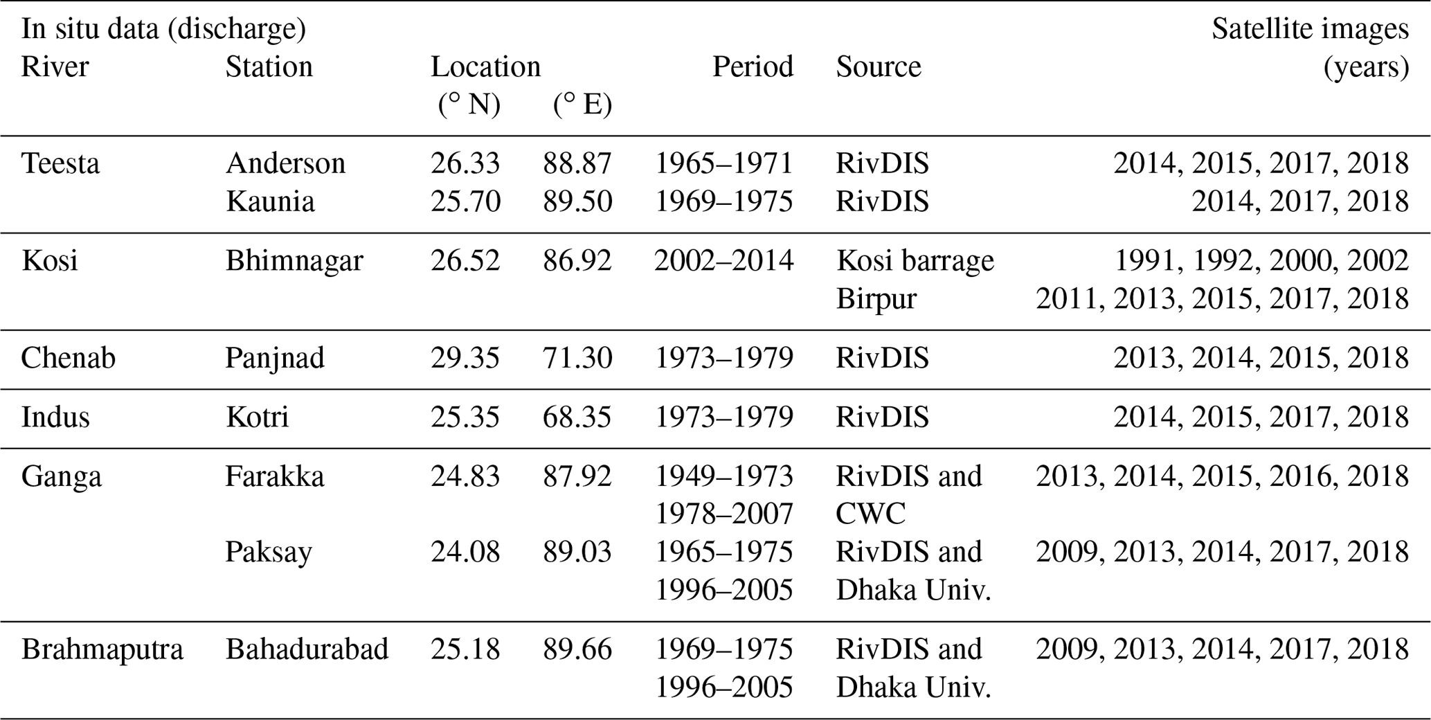
In situ measurements of average monthly discharge for time intervals of varying lengths between 1949 and 1975 are available for the Brahmaputra, Teesta, Ganga, Chenab, and Indus rivers of the Himalayan foreland. They can be freely downloaded from http://www.rivdis.sr.unh.edu/maps (last access: July 2015). We obtained discharge data for the 1996–2005 period for the Ganga River at Paksay station and the Brahmaputra River at Bahadurabad station from Bangladesh. Similarly, the Ganga River discharge from 1978 to 2007 measured at the Farakka station in India was obtained from the Central Water Commission, Ministry of Water resources, New Delhi. We also obtained discharge data for the Kosi River for the 2002–2014 period from the Investigation and Research Division, Kosi River Project, Birpur, and from our own field measurements (Appendix A2). We obtained the median grain size of the bed sediments of the Kosi, Teesta, and Ganga rivers from our own field measurements, whereas measurements for the Chenab, Indus, and Brahmaputra rivers were obtained from the published literature (Goswami, 1985; Dade and Friend, 1998; Gaurav et al., 2017; Khan et al., 2019). The median grain size (d50) of our rivers varies in a narrow range between 250 and 115 µm.
4.2 Width extraction
Our main objective is to extract the width of individual river channels from satellite images. We have developed an automated program in Python 3.7 that takes a greyscale image as input to classify the image pixels into binary water and non-water classes. The pixels classified as water are the foreground object and will be used to define river channels. Dry pixels serve as a background object. To extract the river channels, we use the infrared bands of Landsat TM and Landsat 8 images. In Landsat TM, the infrared (0.76–0.90 µm) wavelength corresponds to band 4, whereas in Landsat 8, it corresponds to band 5 (0.85–0.88 µm). The spatial resolution of the infrared band for both Landsat (TM and 8) missions is 30 m (pixel size: 30 m×30 m). Theoretically, as water absorbs most of the infrared radiation, it appears dark, with an associated brightness value close to zero. This typical characteristic of the infrared signal allows a clear distinction between water-covered and dry areas on satellite images (Frazier and Page, 2000). However, in the case of a river, the pixel intensity varies widely because of heterogeneous reflectance of river water due to the presence of sediment and organic particles (Nykanen et al., 1998). Because the image intensity is not exactly zero or one, we introduce a threshold intensity to classify the pixels. Based on this criteria, we convert the greyscale image f(x,y) into a binary image g(x,y), which distinguishes between the water-covered and dry areas. This approach takes an object–background image and selects a threshold value that segments image pixels into either object (1) or background (0) (Ridler and Calvard, 1978; Sezgin and Sankur, 2004).
We apply the algorithm proposed by Yanni and Horne (1994) to obtain the threshold value iteratively. Once this optimal value is obtained, we apply it to classify our pixels into water and dry classes (Fig. 4). The binary classification of satellite images into water and dry pixels can also produce spurious features (Fig. 4).
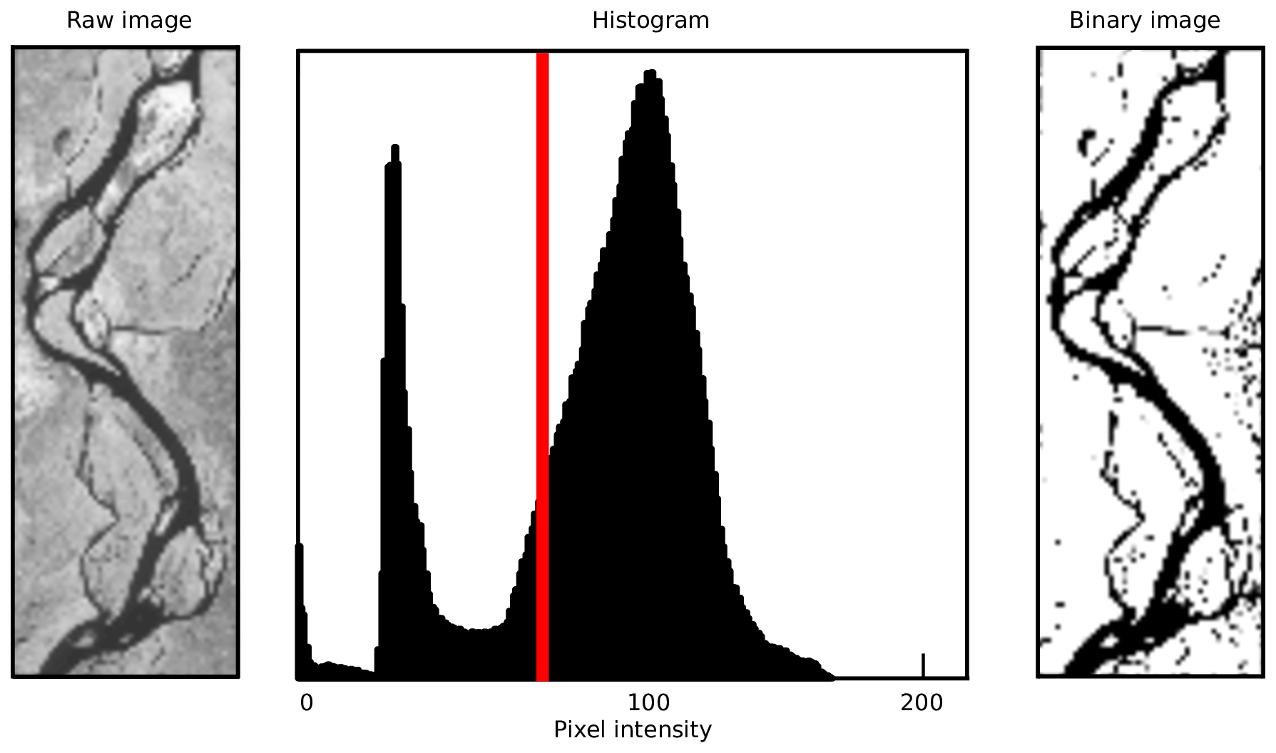
Figure 4Histogram showing the distribution of pixel grey level intensity values. The optimal threshold (T) value (marked with red line) is obtained from the iterative threshold selection algorithm.
These consist of wet pixels that get classified as dry or of isolated water pixels that appear randomly in the binary images (Passalacqua et al., 2013). Clusters (usually two–three pixels in size) that appear inside the river network do not correspond to bars or islands. We found frequent areas where strong reflection from the bed sediment causes water pixels to appear more like sand. Isolated water pixels that do not belong to the river are located in waterlogged areas. We identify these types of errors and reprocess the binary images to remove them automatically. Thus, we first identify the isolated water patches from the binary images; to do this, we define a 7×7 pixel search window. We run this window on the image and look for neighbouring water pixels in all surrounding directions. If a water pixel in the classified image is disconnected in all directions from the neighbouring water pixels for more than seven pixels, we consider it to be an isolated water body. Therefore, we reclassify such pixels as dry. We reiterate this procedure by applying a region-growing algorithm (Mehnert and Jackway, 1997; Bernander et al., 2013; Fan et al., 2005). For this, we initially select a water seed pixel inside the river channel. The algorithm uses the initial water pixels and starts growing. This procedure removes all isolated water patches from the binary image and retains only water pixels connected to the river network.
Once images are reclassified, we reprocess them to merge the water pixels that were initially classified as dry inside a river channel. For this, we define a 3×3 pixel search window. We choose this size by assuming that dry pixels should be more than 90 m in size to be considered as bars or islands. Otherwise, such pixels are treated as water pixels. We move the search window on the binary image and look for neighbouring dry pixels inside the river channel.
Similarly, to identify river pixels from Sentinel-1A images, we use the VH (vertical transmission and horizontal reception) polarised band. The Sentinel Application Platform (SNAP) v6.0 performs the radiometric calibration, speckle noise reduction using a refined Lee filter, and terrain corrections, and finally generates the backscatter (σ0) image. This image has a 60 m×60 m pixel size that we resampled at 30 m×30 m to be consistent with the pixel size of Landsat images. In the microwave region, open and calm water bodies exhibit low backscatter values due to high specular reflection from the water surface (Schlaffer et al., 2015; Twele et al., 2016; Amitrano et al., 2018). We manually set a threshold value to separate water and dry pixels from Sentinel-1 images. Finally, we follow a similar procedure to the procedure that we developed for Landsat images to process the binary image obtained from Sentinel-1.
Once the satellite images are classified, we use the binary images to extract the width of each channel. We do this by measuring the distance from the centre of a channel to its banks, orthogonal to the flow direction. A detailed automated procedure of the width extraction of a river channel is given in Appendix B.
5.1 Accuracy assessment
To assess the precision with which we can estimate the discharge of a thread, we need to quantify the accuracy of our width extraction procedure using Landsat and Sentinel-1 satellite images. To evaluate this, we superimpose the contours of river channels, extracted using our algorithm, to the original greyscale images used for the extraction. We then carefully check for a match between the contours' boundary and water boundary in the greyscale image. We observed a good agreement between the automatically extracted channel boundary and the edge of the water line in the greyscale image. However, our algorithm fails to extract the contours of the smallest channels (60–90 m in width). There are several explanations for this limitation. First, as these channels are shallow and only a few pixels wide, their pixel intensity is close to the pixel intensity of dry areas. Therefore, the optimal threshold applied to categorise the image pixels does not identify these channels as water. Second, although an increase in the classification threshold could force the algorithm to identify these pixels as water, it would also add significant noise by classifying many dry pixels as water pixels. Such a limitation appears to be closely related to the image resolution.
Given this qualitative agreement, we proceed to evaluate the accuracy of the width extraction procedure. To do this, we overlay the transects used by the algorithm to measure the width of a thread on the original image (Fig. 5a).
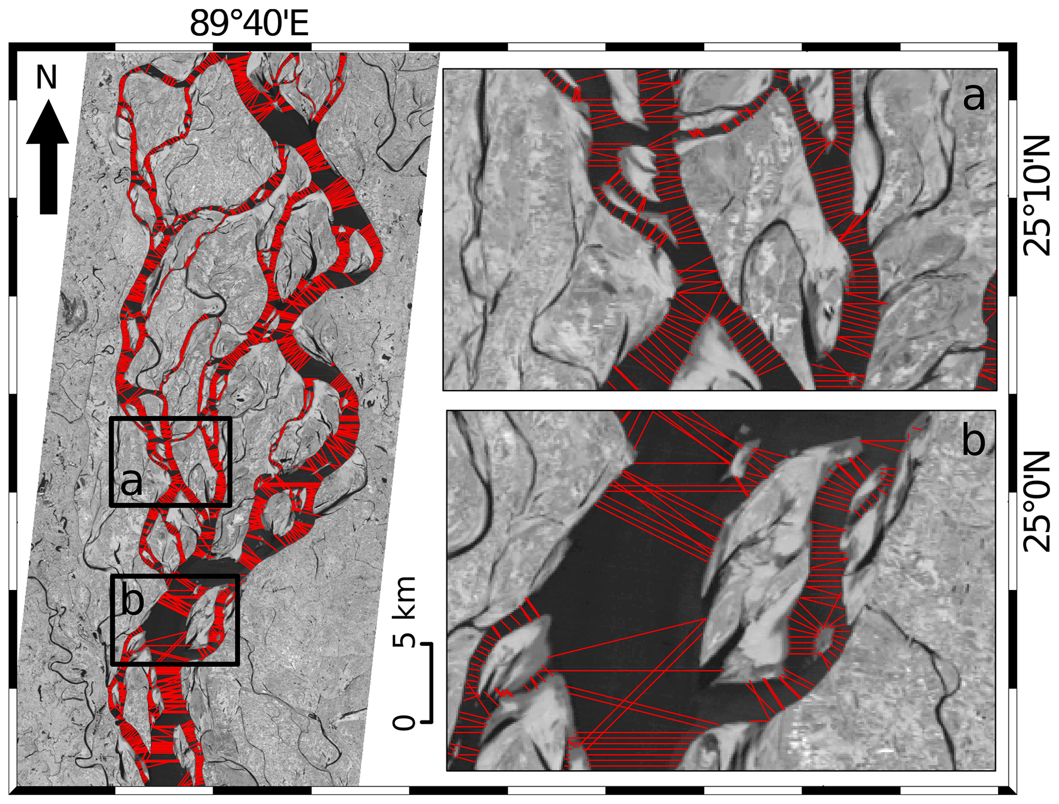
Figure 5Width of the individual threads estimated across different transects along a reach of the Brahmaputra River from Landsat satellite image. Panels (a) and (b) illustrate the regions of valid and erroneous transects at different places in the river (image source: Landsat TM, 29 November 2013).
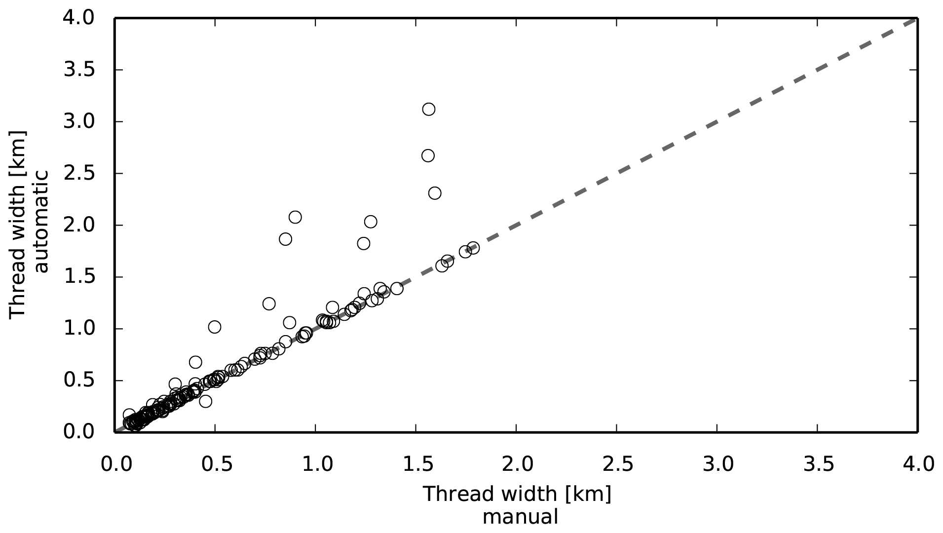
Figure 6Thread widths extracted using the automated technique are plotted as function of the manually extracted width.
We then manually measure the width at randomly selected transects for comparison. For each river, we manually measure the width at more than 15 randomly selected transects. We then compare the automatically extracted and manually measured widths.
Figure 6 compares the widths extracted automatically and manually. Most of the data points cluster on the 1:1 line. This indicates that, for the vast majority of threads, the width computed from our automated procedure is almost equal to the width measured manually.
However, there are some outliers. These outliers correspond to locations along the threads where our automated procedure draws erroneous transects (Fig. 5b). Most of these transects are located near highly curved reaches at the confluence or diffluence of two or more threads. In such places, the width of a thread is overestimated, sometimes by more than 50 %, compared with the manually measured width. At most locations though, our procedure extracts valid transects (Fig. 5a).
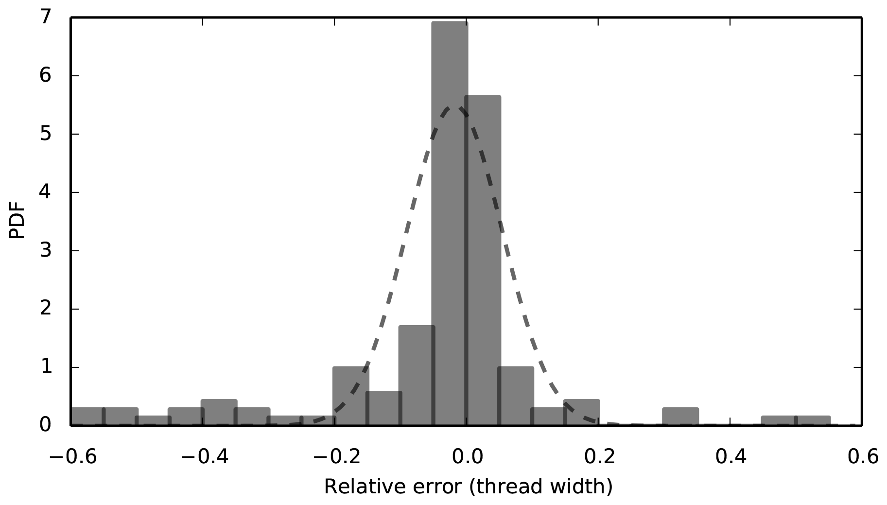
Figure 7Distribution of the error in the thread widths extracted automatically. The corresponding normal distribution is obtained by removing the 10 % extreme values from the distribution.

Figure 8Spatial distribution of the width measured along the threads of a braided reach of the Ganga River near the Paksay gauging station in Bangladesh. The vertical line (red) on the histograms in panels (a) and (b) represents the geometric mean that corresponds to the most probable width (Wm).
Furthermore, we assess the distribution of relative discrepancies between automatically and manually measured widths (Fig. 7). To quantify the precision of our measurements, we compute the relative error. We observe that the relative error of 90 % of our measurements is centred around a mean with a standard deviation σ≈0.07. This validates the width extraction procedure.
5.2 Width variability along a thread
Particularly in a braided river, the width of a thread varies significantly along its course. To quantify this variability, we select a reach and plot the probability distribution of the width measured across different transects. We observed that the distribution of width histograms is skewed (Fig. 8). This skewness results from the natural variability in width along the course and also due to the error in width extraction from images, particularly at locations where the curvature of a thread is high. The resulting skewness will be amplified in the discharge histogram because of the non-linear relationship relating the two variables. To take the skewness into account, we have calculated the geometric mean of all of the measured values. The geometric mean is less affected by extreme values in a skewed distribution and can be considered a representative width (Wr). However, in meandering rivers where there is not much variability in width within a reach, the arithmetic mean can be considered a representative width.
5.3 Discharge estimation
We now proceed to estimate discharge (Qw) for the Himalayan rivers based on their channel widths extracted from satellite images. To have a meaningful comparison between the image-derived discharge and the corresponding in situ measurement, we select a reach about 10 times longer than the width of a river on satellite images. In the case of a braided river, we consider the widest channel to define the reach length. In the selected reach, we assume that discharge is conserved: there is no significant addition or extraction of water in the river.
To estimate the discharge of the study reach, we use a regime relation established by Gaurav et al. (2017) based on threshold channel theory (Eq. 4) and field measurements of a channel's width and discharge on the Ganga–Brahmaputra plains. The resulting regime relation is governed by
where α is the best-fit coefficient, an empirical value obtained from fitting the prefactor of the regime curve (Eq. 4), Wr is the representative width, and ds is the median grain size.
We use Eq. (6) to calculate the discharge for threads of known width. Because the river width scales non-linearly with discharge, the regime relations obtained refer to the total width in the case of a braided river, and they will not be the same as those obtained for individual threads. As most of the studied rivers are braided, we first calculate the discharge for individual threads across a given section. We then sum the discharge of the individual threads across a transect to compute the total discharge at a section.
5.4 Estimated vs. measured discharge
Once monthly discharges for all of the rivers are estimated from satellite images, we compare them with the average monthly discharge measured at the corresponding gauging stations. To do so, we plot the hydrographs of the estimated and measured discharges together (Fig. 9). We observed that the estimated discharge of the Kosi, Ganga, and Brahmaputra rivers from satellite images is overestimated and almost constant throughout during the non-monsoon period (October–May). Conversely, the Indus, Chenab, and Teesta rivers show a clear annual cycle. This observed trend is not entirely clear to us, but it could possibly be related to the flow regulation, as these river are highly regulated through a series of dams and barrages.
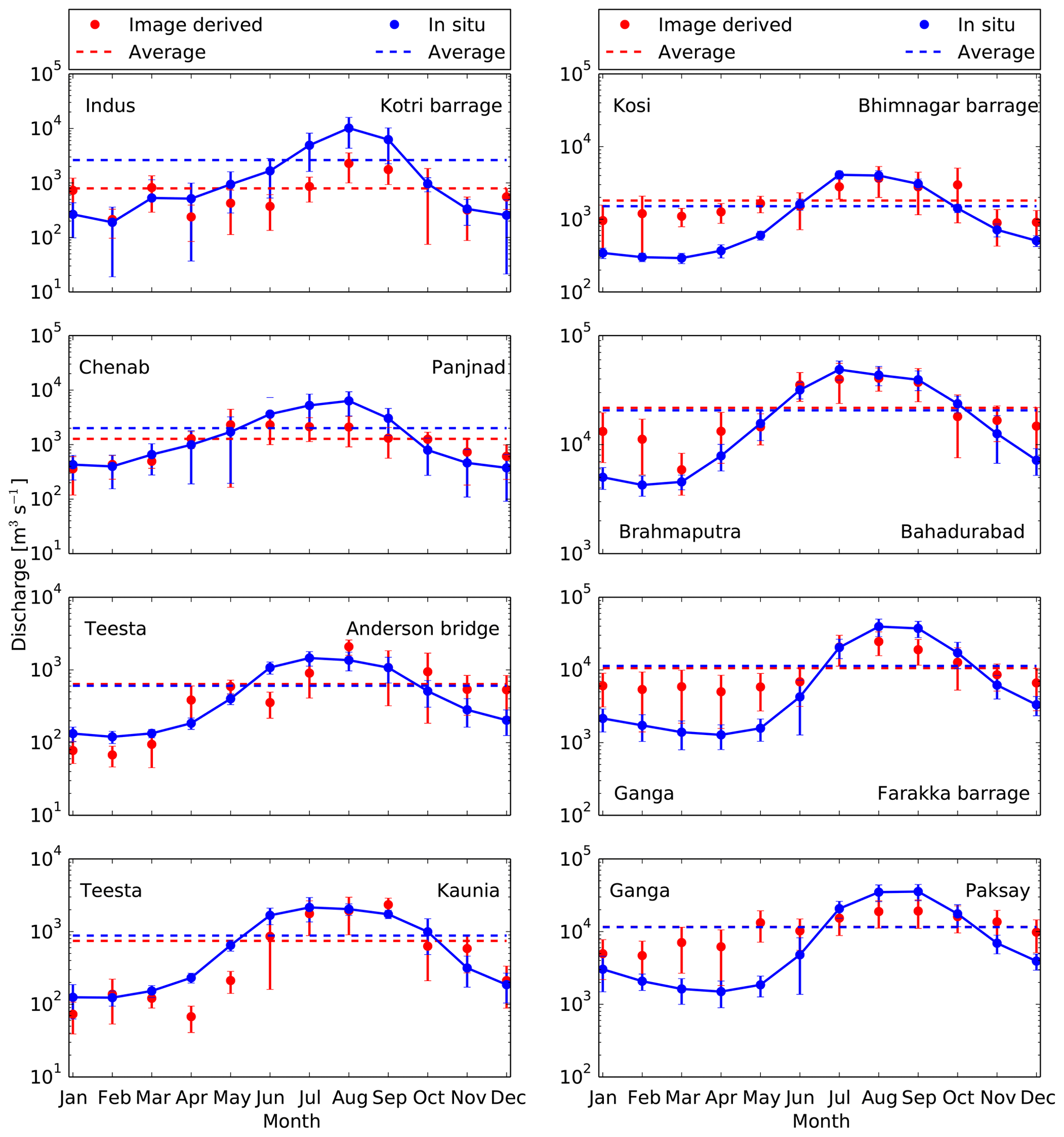
Figure 9Hydrograph of satellite-derived reach-averaged discharge against their monthly average discharge recorded at the gauging station. The error bar in the measured discharge (blue) is the standard deviation calculated from the time series of different months; the error bar in the estimated discharge represents the standard deviation within the study reach. Dotted red and blue lines are the annual average discharge obtained from satellite images and in situ measurement respectively.
Furthermore, we observed that the estimated discharge for most of our rivers show a significant rise during the monsoon period (June–September). To the first order, it appears that our approach is able to capture the rising trend of discharges during the monsoon period; however, the estimated discharges are lesser than the measured discharges. Table 2 compares the estimated and measured discharges during the monsoon period. For most of our rivers, the difference between measured and estimated discharges is less than 50 %, although this difference is comparatively high for the Indus (72 %–78 %) and Chenab (36 %–67 %) rivers (Table 2).
Table 1Comparison between the image-derived discharge and the discharge measured in situ for the Himalayan rivers during the Indian summer monsoon period. The error in the measured discharge is the standard deviation calculated from the time series of different months; the error in the estimated discharge is the standard deviation within the study reach.
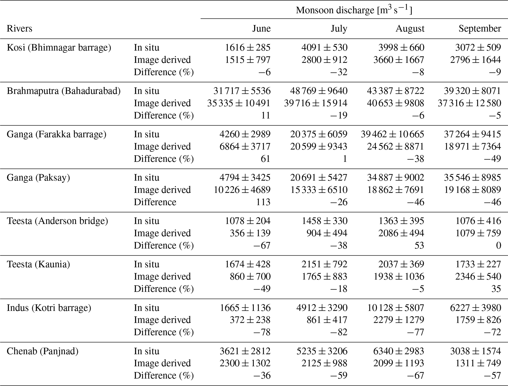
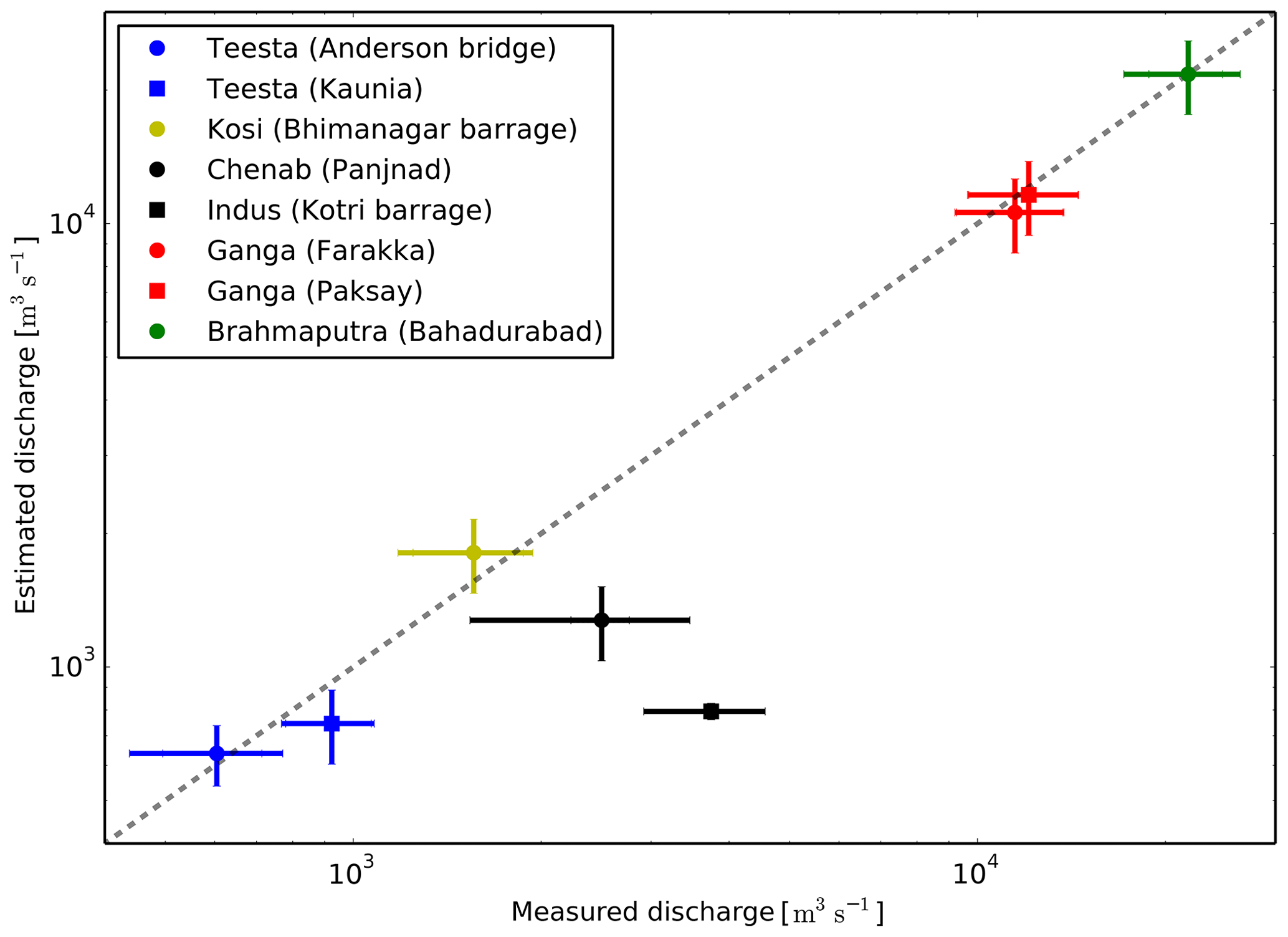
Figure 10Satellite-derived river discharge against annual average discharge measured at a ground station. The error bar in the measured discharge represents the standard deviation; the error bar for the estimated discharge is calculated by considering ±10 % measurement uncertainty in the channel widths from satellite images.
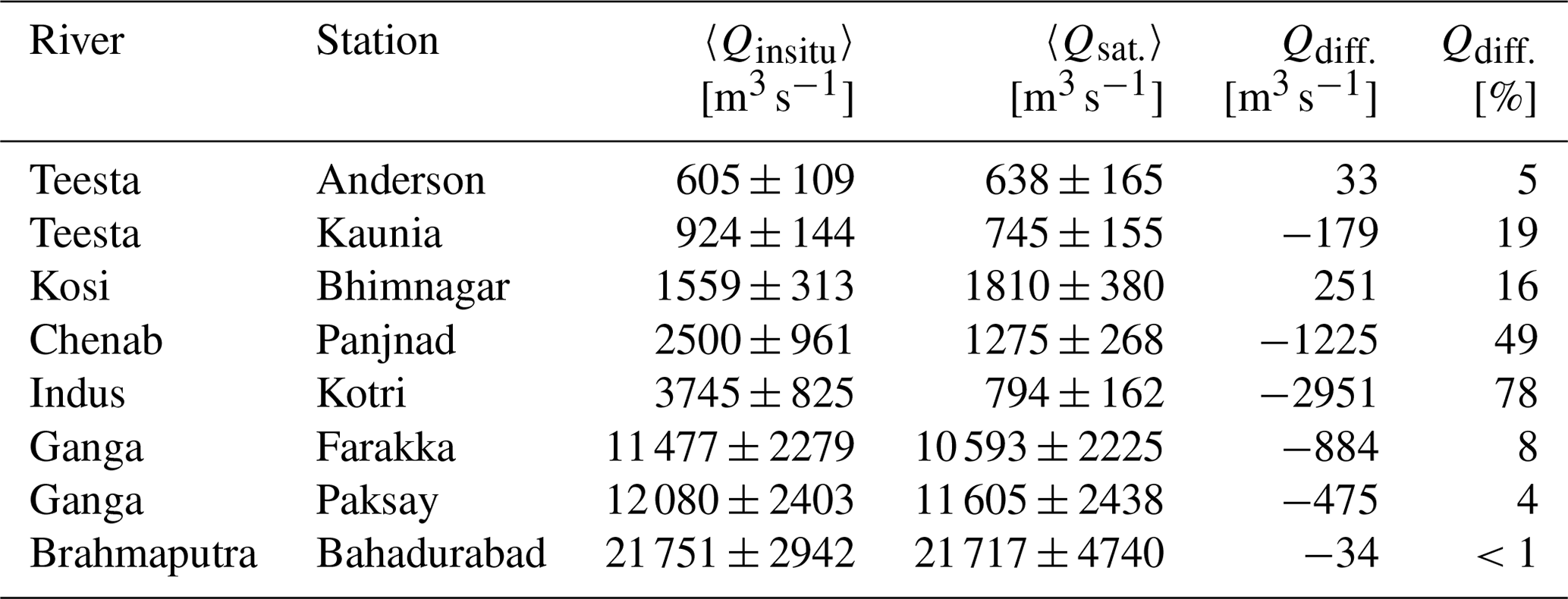
Table 2Comparison between the annual average discharge measured at the gauging stations and that estimated from satellite images.
It is important to note that the discharge estimated from satellite images does not correspond to an instantaneous discharge. To understand the emergence of a constant hydrograph from the estimated discharge derived from satellite images, we explore the concept of channel-forming (formative) discharge, i.e. a discharge that sets the geometry of alluvial river channels. Several workers, including Inglis and Lacey (1947), Leopold and Maddock (1953), and Blench (1957), have shown that the geometry of an alluvial channel corresponds to a formative discharge (see Table A2 in the Appendix for the definition of different discharges). They have discussed how a limited range of flows are responsible for shaping its channel. At low-flow discharge, the water simply flows through the threads without affecting their geometry. Schumm and Lichty (1965) used the concept of time span (geologic, modern, and present) in defining the interrelationship between dependent and independent variables of a river system. According to these authors, the morphology of a river channel is set in the modern time span (last 1000 years) by the average discharge of water and sediment. In the present time span (1 year or less), channel morphology can be considered as an independent variable against instantaneous discharge of water and sediment.
Similarly, it has been argued by Inglis and Lacey (1947), Leopold and Maddock (1953), and Blench (1957) that it is not the highest flows that contribute the most in shaping a river channel. Such high discharges are capable of transforming the channel, but they occur so infrequently that, on average, their morphological impact is small. Wolman and Miller (1960) highlighted that the bankfull discharge that occurs once each year or every 2 years sets the pattern and channel width of the alluvial rivers. Formative discharge for the Himalayan rivers is expected to occur in the monsoon period; thus, during low flow, one may expect that such rivers maintain their flows without modifying the existing channel geometry (Roy and Sinha, 2014). This is clearly reflected in the discharge hydrographs estimated from the measurement of channels' width from the satellite images (Fig. 9). Furthermore, Métivier et al. (2017) have recently shown that non-cohesive streams laden with sediments cannot have a width much larger than the width of a threshold stream before they start to braid. They also showed that, for experimental braided rivers, threads are always formed at the bankfull flow and at the limit of stability. Thus, our hypothesis is that the formative discharge of threads in the Ganga plain is the bankfull discharge. This is probably why our estimated discharge from satellite images remain constant throughout the non-monsoon period for most of the rivers and is mostly overestimated compared with the measured discharge at gauging stations.
According to Inglis and Lacey (1947), rivers approach their equilibrium geometry for a formative discharge that approximately corresponds to the bankfull discharge. They suggested this discharge lies between half and two-thirds of the maximum discharge. It has also been suggested that the formative discharge corresponds to the median discharge (Blench, 1957). In their study, Leopold and Maddock (1953) used the discharge that corresponds to a given frequency of occurrence and compared it to the hydraulic geometry of the river. Based on their observations in the US, they recommended the use of the annual average discharge as a proxy for the formative discharge. Hereafter, we use the definition of Leopold and Maddock (1953).
Based on our understanding of the geometry of alluvial river channels, we argue that the width of the thread that we extract from satellite images corresponds to a formative discharge. As discussed by Gaurav et al. (2014), the high-resolution bathymetry profile of a braided thread reveals the complex topography of the bed. As an example, Fig. C1 in the Appendix, illustrates the cross section of a braided thread measured in the field using an acoustic Doppler current profiler (ADCP). This high-resolution bathymetric profile enables us to identify the two different threads separated by submerged bars and islands. In such situations, discharge is not carried across the width seen from the plan view but only through the narrow active regions. Furthermore, this indicates that during low flow, water spread in the existing geometry is set at the formative discharge. Currently, satellite images allow us to measure the top width of the water surface. For a given thread, we presume that discharge estimated from these widths should compare to the formative discharge.
We now evaluate how the discharge estimated from satellite data varies with time. We plot the monthly discharge estimated for all of our rivers to their corresponding average monthly discharge measured at the gauging stations (Fig. 9 in the Appendix). The monthly average discharge of the Himalayan foreland rivers appears to be a representative of the actual hydrograph (Fig. C2). As suggested earlier by Inglis and Lacey (1947), Leopold and Maddock (1953), and Blench (1957), we observe that except for the Indus, Chenab, and Teesta rivers, the estimated discharges from images are nearly constant throughout during the non-monsoon period, with small fluctuations around their mean. This supports the hypothesis that the width of the thread extracted from satellite images corresponds to a value closer to the formative discharge.
To extend upon this, we now compare the annual average discharge estimated from Landsat and Sentinel-1A images for different months to the annual average discharge measured at corresponding ground stations. We plot these discharges on a log–log scale (Fig. 10). The discharge estimated from satellite images agrees to within an order of magnitude with the measured discharge.
The differences between the measured and estimated annual average discharges for the Brahmaputra, Ganga, Kosi, and Teesta rivers are less than 20 %. However, this difference is comparatively high for the Indus (78 %) and Chenab (49 %) rivers. Interestingly, the estimated discharges for the Teesta (at Anderson station), Ganga (at Farakka and Paksay), and Brahmaputra (at Bahadurabad) rivers converge to their measured discharges with small differences of 5 %, 8 %, 4 %, and <1 % respectively (Table 2); in contrast, the estimated discharges of the Teesta (at Kaunia station) and Kosi (at Bhimnagar) show a relatively higher differences of 19 % and 16 % respectively. These differences could possibly be related to the anthropogenic impact on the natural flow condition. For example, the selected study reaches for the Teesta (at Kaunia station) and Kosi (at Bhimnagar) rivers are located near the barrage where flow is regulated. However, this relationship is not entirely clear at this stage.
Similarly, the observed annual cycle in discharge and the large difference between the estimated and measured discharge of the Indus and Chenab rivers could possibly be related to a series of dams and barrages (Kotri barrage, 1955; Mangla dam, 1967; Tarbela dam, 1976) that have been constructed. Such anthropogenic intervention has significantly altered the water and sediment discharge of the Indus River. For example, downstream of the Kotri barrage, the average annual water discharge of the Indus River has declined at an alarming rate from about 107×109 m3 to 10×109 m3 from 1954 to 2003 (Inam et al., 2007). This continuous decline in the average annual discharge might have significantly modified the geometry of the Indus River.
Furthermore, to understand our estimates of discharge for the Chenab, Indus, and Teesta rivers, we plot their monthly discharge time series recorded at the corresponding gauging stations against the discharge estimated from satellite images (Figs. C3 and C4 in the Appendix). Despite a large variability, the discharge time series of the Indus and Chenab rivers show a strong declining trend during the monsoon period (June–September), whereas discharge during the non-monsoon period appears to remain constant around the mean value. Figure C3 in the Appendix clearly shows that discharge estimated from satellite images plots within the variability of the observed trend. The estimated discharge of the Teesta River also plots within the noise of the observed trend. This gives us confidence in our estimates of discharge, especially for the rivers for which we have a limited, old record (1973–1979) of in situ discharges.
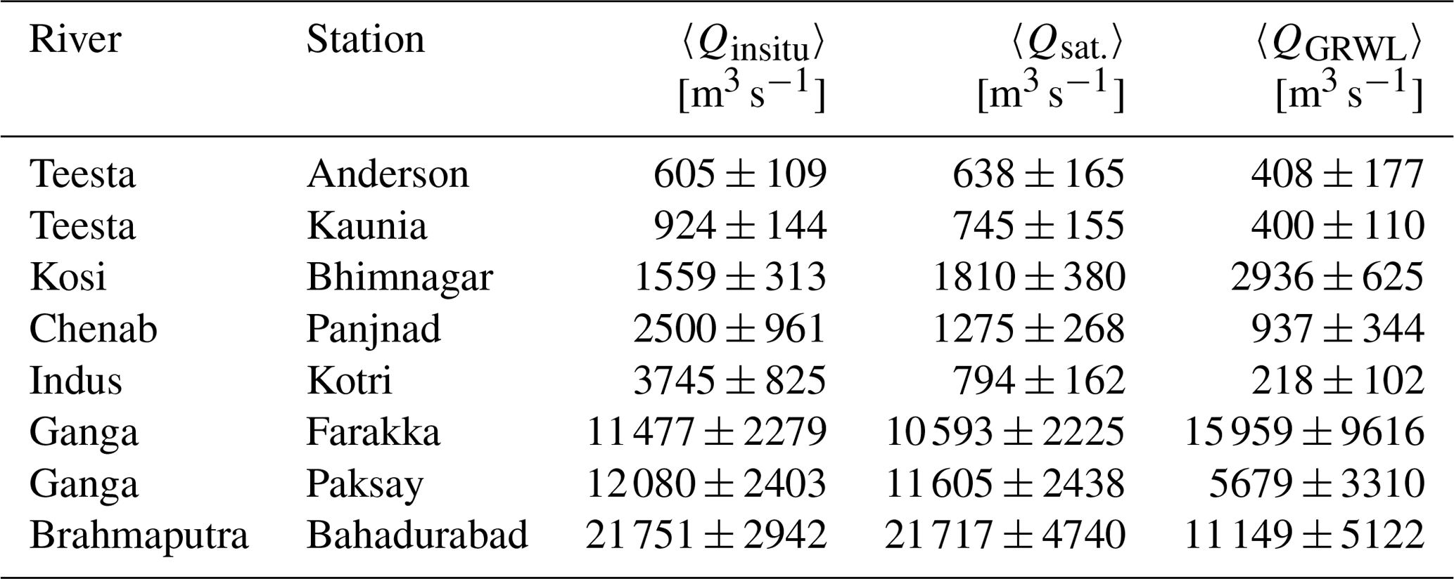
In a recent study, Allen and Pavelsky (2018) measured the width of the global rivers from Landsat images for the month when they commonly flow near mean discharge. We have used the water mask binary images from the Global River Width from Landsat (GRWL) database and measured the thread widths of the Brahmaputra, Chenab, Ganga, Indus, and Teesta rivers (Appendix C). We used these widths to estimate discharges using our regime curve and compare them with the mean annual discharge recorded at the corresponding gauging station as well as our estimates from satellite images. For most of our rivers, we observed that the discharge estimated from the thread's width extracted from the GRWL database of Allen and Pavelsky (2018) falls within the same order of magnitude as the yearly average discharge measured at the corresponding gauging stations (Table C1). For most rivers, the difference between the measured and estimated discharge from GRWL data is approximately less than 60 %. However, this difference is comparatively high for the Kosi (88 %) and Indus (95 %) rivers. Interestingly, in accordance to our estimates, the GRWL database also shows a high reduction in the discharge of the Indus and Chenab rivers from the measured discharge at their corresponding ground stations during the period from 1973 to 1979.
The GRWL database is a first ever compilation of width for the global rivers, and it may be used together with our regime curve to obtain a first-order approximation of the formative discharge of the Himalayan foreland rivers.
The semi-empirical regime relation established by Gaurav et al. (2017) and remote sensing images can be used to obtain a first-order estimate of the formative discharge of the rivers of the Himalayan foreland, if their channel width is known. The regime equation used here is established from the recent measurements and the published data by Gaurav et al. (2014, 2017). This equation is based on threshold theory and instantaneous measurements of the hydraulic geometry of individual threads of various braided and meandering rivers. The measurements were acquired during the period when rivers of the Himalayan foreland usually flow at their formative discharge (Roy and Sinha, 2014). Therefore, this regime equation only provides an estimate of the formative discharge, and it can not capture the instantaneous variations in discharge. On the other hand, as this regime relation is established from the measurements in braided and meandering rivers, it can be used to establish first-order estimates of formative discharge in a river of any planform. It is especially useful and relevant for braided rivers that present several difficulties with respect to the measurement of discharge in the field. Our regime equation requires only one parameter (grain size) to estimate discharge from width measurements. It can be obtained easily from field measurements. As our regime equation is established from measurements of a wide range of channels spanning over the Ganga and Brahmaputra plains, we believe that it can be used to obtain a first-order estimate of the formative discharge of rivers in the Himalayan foreland by just measuring their channel width on satellite or aerial images. Using our semi-empirical regime equation and satellite images of the Landsat and Sentinel-1 missions, we have estimated the discharge of six major rivers in the Himalayan foreland (Brahmaputra, Chenab, Ganga, Indus, Kosi, and Teesta). Our estimated discharges closely compare with the average annual discharge measured at the nearest gauging stations. This first-order agreement, although encouraging, requires further research to improve the degree of agreement between measured and estimated discharges. One of the main sources of uncertainty in the discharge estimate is due to the error in the measurement of thread widths. This depends on the image resolution and accuracy of the algorithm used for the extraction of river pixels from remotely sensed images. Better-resolution remote sensing images would most likely minimise the uncertainty and improve the agreement between estimated and in situ discharge. Furthermore, our regime equation established for the Himalayan rivers is based on a simple physical mechanism that explains the geometry of alluvial channels. Therefore, we suspect that the procedure we have established could be extended to most alluvial rivers. Globally, it has been observed that the threshold theory well predicts the exponent of the regime equation (Eq. 6); however, the prefactor may vary significantly depending on the grain size distribution, the turbulent friction coefficient, and the critical Shields parameter (Métivier et al., 2017). It is, therefore, suggested that this regime curve is modified using measurements of the width, discharge, and grain size of individual threads of alluvial channels in the field before applying it to rivers with different climatic regimes. Moreover, it should be noted that our regime curve relates to the measurement of hydraulic geometry of individual threads of braided and meandering rivers; therefore, it is applicable only at the thread scale. As the resulting regime curve is non-linear, estimating discharge across a transect in a braided river from the aggregated width will be different from the discharge obtained after the summation of discharges of the individual threads.
This study presents a robust methodology and is a step towards obtaining first-order estimates of formative discharge in ungauged river basins solely from remote sensing images. It can be used for sustainable river development and management to ensure regional water security and flood management, especially in regions where river discharge data are not readily available.
A1 Satellite images
In this section, a detailed specification of the satellite data (Landsat and Sentinel-1) used in this study is given.
Table A1Details of the Landsat 8 (L-8), Landsat TM (L-TM), and Sentinel-1A (S-1A) satellite images used in this study. “Gauging station” is the location (∘ N, ∘ E) of the nearest in situ discharge measurement station.
A2 Description of satellite and in situ dataset
Table A1 contains a detailed description of in situ discharge data for the different rivers used in this study. This includes the data source, the location of the gauging station, and the period of measurement.
Table A2Satellite images used for the extraction of the channel widths. In situ discharge data are freely available and were downloaded from http://www.rivdis.sr.unh.edu/maps/asi/ (last access: 19 July 2015).
A3 Glossary
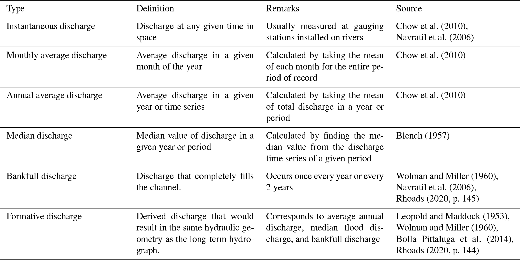
Chow et al. (2010)Navratil et al. (2006)Chow et al. (2010)Chow et al. (2010)Blench (1957)Wolman and Miller (1960)Navratil et al. (2006)Rhoads (2020, p. 145)Leopold and Maddock (1953)Wolman and Miller (1960)Bolla Pittaluga et al. (2014)Rhoads (2020, p. 144)Table A3A summary of the terminology used for different discharge types used in this study.
B1 Identification of river channels
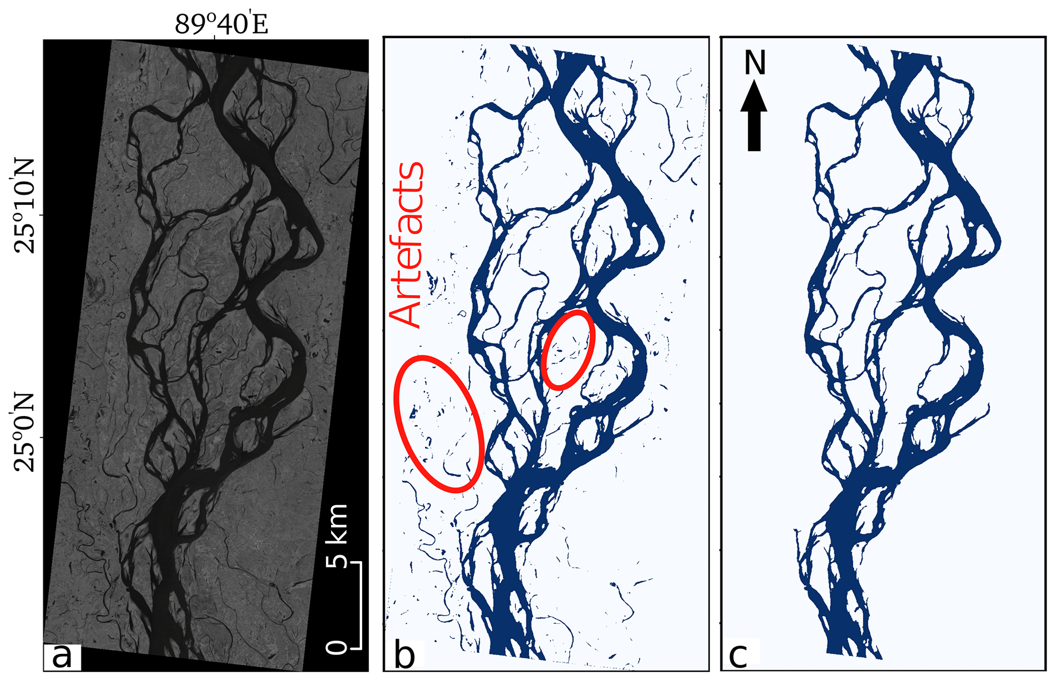
Figure B1(a) A threshold intensity value is applied on the input greyscale image (SWIR) of Landsat 8 to obtain a binary image with water (blue) and dry (white) pixels. (b) Binary images with isolated water patches and artefacts and (c) removed artefacts (image source: Landsat TM, 29 November 2013).
To identify the river and non-river pixels, we used the infrared bands of Landsat TM and Landsat 8 images. In Landsat TM, the infrared (0.76–0.90 µm) wavelength corresponds to band 4, whereas in Landsat 8 image, it corresponds to band 5 (0.85–0.88 µm).
We obtained an optimal threshold value by using the algorithm initially proposed by Yanni and Horne (1994). We then used the optimal threshold value to separate water and dry pixels from Landsat satellite images. The algorithm is initiated by selecting a threshold as a midpoint value that lies between the maximum and minimum grey level intensity (gi) as follows: , where gimax is the highest and gimin is the lowest grey level intensity. Based on this initial threshold, the image pixels are clustered into foreground and background objects. After each iteration, the threshold value is updated using the mean intensity of both the clusters. Finally the algorithm terminates when the threshold converges.
B2 Removal of artefacts
Thresholding a greyscale input satellite image into binary class (water and dry pixels) produces spurious features. These consist of wet pixels that are classified as dry pixels or of isolated water pixels that appear randomly in the binary images. Clusters (usually two–three pixels in size) that appear inside the river network do not corresponds to bars or islands. They appear to be more frequent in the areas where strong reflection from the bed sediment cause water pixels to appear more like a sand. Isolated water pixels that do not belong to the river are disconnected and located in waterlogged areas. We have identified both of these type errors from binary image and reprocess to remove them automatically. While doing this, we first define a seed point inside the main channel and run the flood-filling algorithm (Mehnert and Jackway, 1997; Bernander et al., 2013; Fan et al., 2005). This identifies water pixels in a river channel that are connected and removes the isolated water pixels that have poor connectivity (Fig. B1).
B3 Extraction of the channel skeleton and contour
Our channel width extraction algorithm requires the river's centreline and boundary. A river centreline, often called skeleton in computer vision, corresponds to its median axis. To identify the river's skeleton, we used a thinning algorithm to extract the centreline. The algorithm iteratively reduces the boundary pixels in a way that preserves its topology (for example, eroding pixels must not alter the geometric properties of the object studied) and connectivity (Fig. B2a). The final skeleton is centred within the object and reflects its geometrical properties (Zhang and Suen, 1984; Baruch, 1988; Lam et al., 1992; Chatbri et al., 2015). The thinning algorithm produces several small centreline segments, often less than 300 m in length, that are disconnected from the channel network at one end. These segments of the skeleton are too small to be considered part of the river network. For our purpose, we consider such segments as noise and filter them out. We do this iteratively by looking for skeleton segments that are disconnected from the skeleton network at one end. To extract the channel banks, we applied a contour extraction algorithm that detects the outer boundary of a channel (Fig. B2). The algorithm relies on a pixel neighbourhood analysis, where a pixel in a binary image is considered a contour pixel if it has at least one background neighbour (Chatbri et al., 2015).
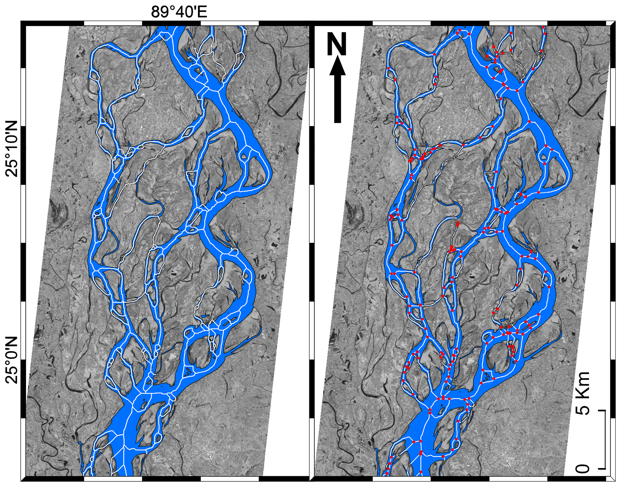
Figure B2The image on the left shows the river centreline (skeleton) and boundary (contour) superimposed on a Landsat 8 satellite image. The image on the right illustrates the stream junction identified on the skeleton (left) image (image source: Landsat TM, 29 November 2013).
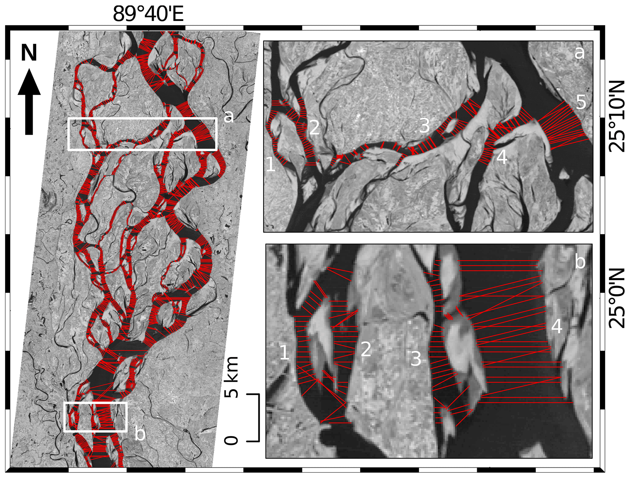
Figure B3The width extracted across each of the individual channels. The image on the right illustrates the reach lengths (in boxes) over which the most probable width of each channel is calculated (image source: Landsat TM, 29 November 2013).
B4 Channel width calculation
Once the satellite images are processed to extract the skeleton and channel banks, we then proceed with extracting the width of each channel. We do this by measuring the distance from the centre of a channel to its banks, orthogonal to the flow. From the skeleton of the image, we draw a perpendicular line to the river bank and measure the Euclidean distance (Fig. B3). For a braided river, especially near junctions where more than two rivers join or bifurcate, this forms a complex network. At such locations, our algorithm fails to measure the correct width. To circumvent this, we identify all of the junctions from the river skeleton (Fig. B2b). We consider an area of five pixels in the proximity of a junction and define them as a zone of channel confluence and diffluence. We then avoid calculating the width of the channels in these zones.
Finally, we draw perpendicular transects from each pixel of the skeleton to both side of the channel and calculate the distance from any point (x,y) on the skeleton to its corresponding left (x1,y1) and right (x2,y2) points on the channel boundary (Fig. B3). We then sum these widths to get the total width across a transect. For simplicity, we compute the most probable width of each channels across a river section at 1 km intervals along the channel. Finally, the discharges through a section can be calculated along an entire reach (Fig. B3).
C1 Cross section of a braided thread
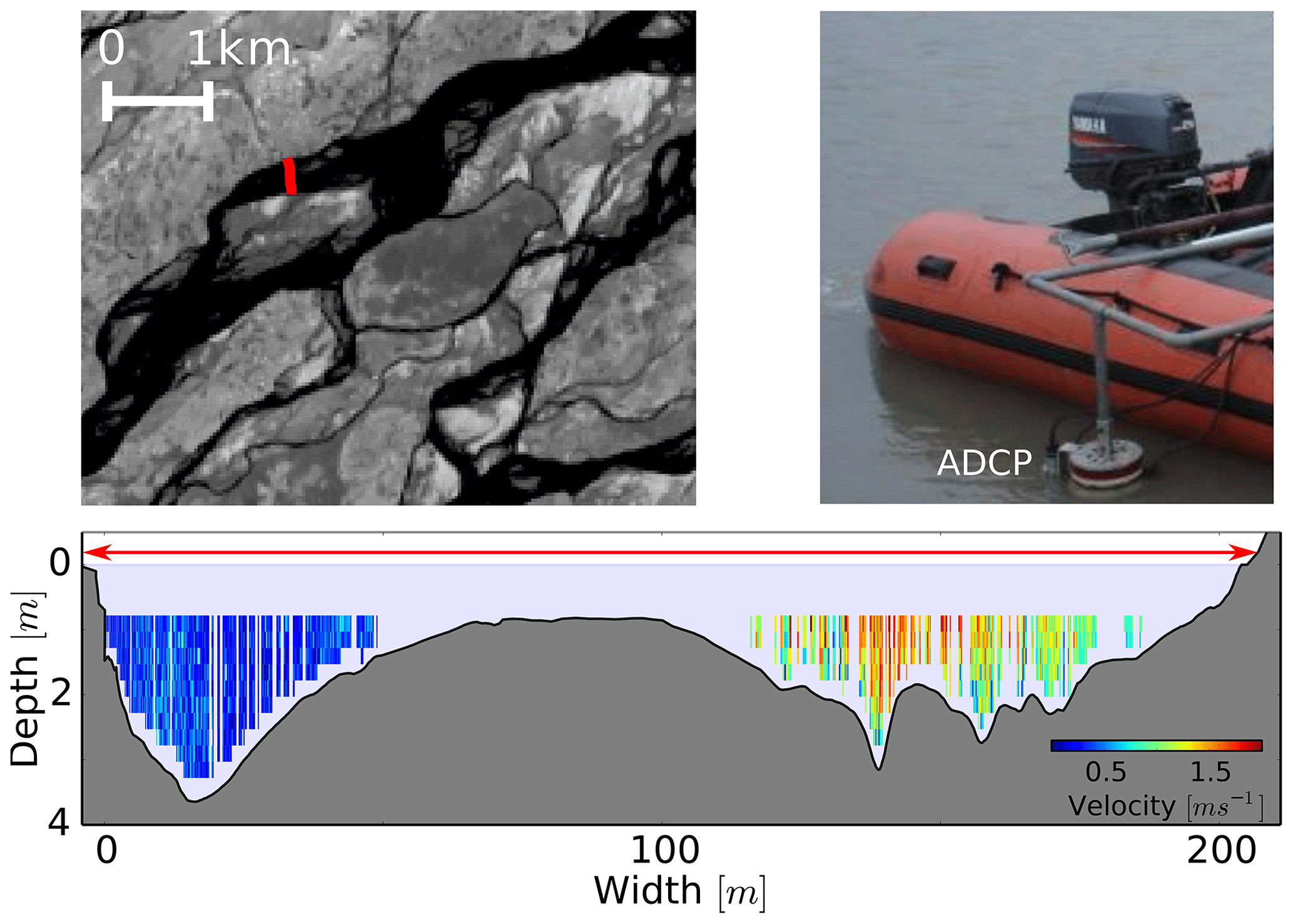
Figure C1Velocity profile measured using the ADCP across a braided thread of the Kosi River in the Himalayan foreland. The red horizontal line with the arrow illustrates the top water surface. Colours of different intensities show the magnitude of velocity (m s−1).
C2 Hydrograph of the Kosi River
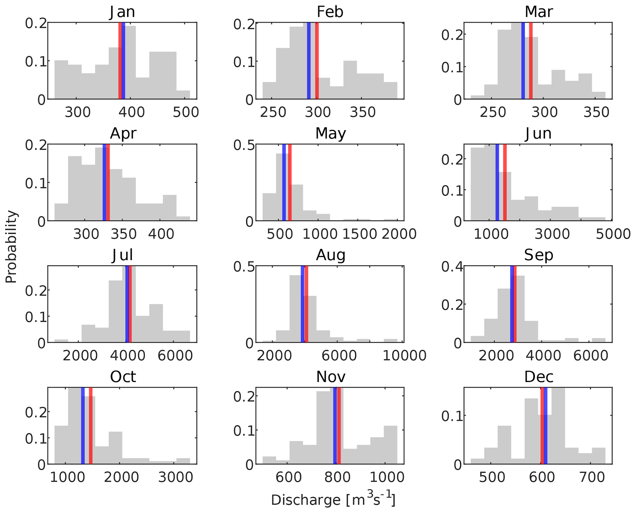
Figure C2Histogram of daily discharge of the Kosi River measured at the Bhimnagar barrage in 2011, 2013, and 2014. Vertical lines in red and blue are the mean and median values of the probability distribution.
C3 Evolution of discharge time series
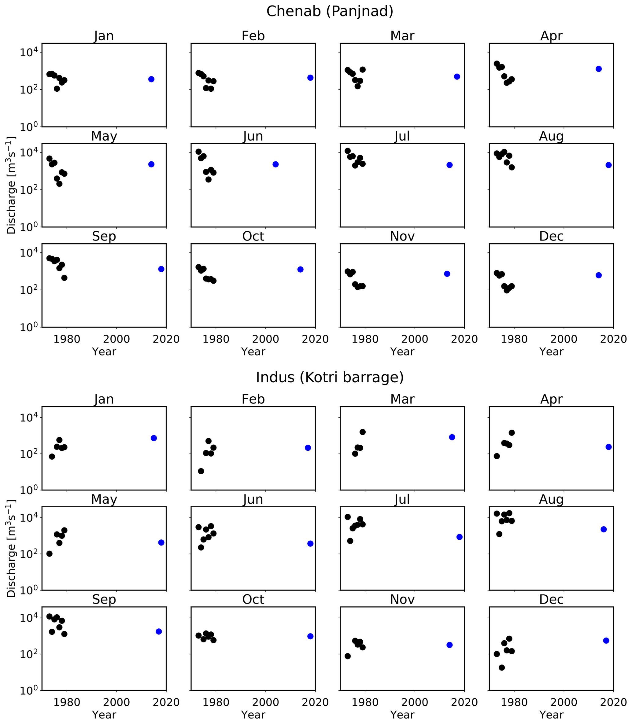
Figure C3Time series of discharge of the Chenab and Indus rivers (black circles) measured at the ground stations (Panjnad and Kotri barrage respectively). The blue circles represent the discharge estimated from satellite images.
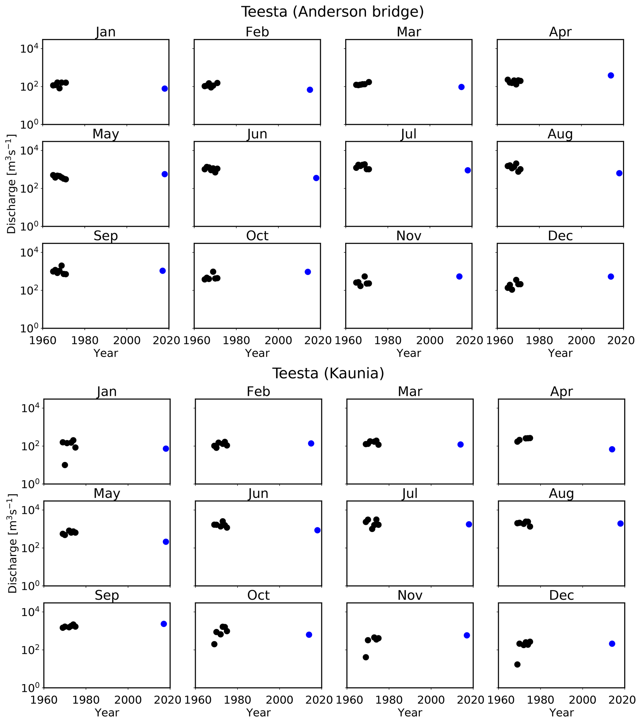
Figure C4Time series of discharge of the Teesta River (black circles) measured at the ground stations (Anderson bridge and Kaunia respectively). Blue circles represent the discharge estimated from satellite images.
C4 Comparison of mean annual discharge with the GRWL database
Allen and Pavelsky (2018) measured the width of global rivers from Landsat images for the month when they commonly flow near mean discharge. In their database, the Global River Width from Landsat (GRWL) database, for braided rivers they reported the aggregated width of all of the active threads. This width can not be used to estimate discharge from our regime curve that we established for the Himalayan rivers. Our regime curve relates to the measurement of hydraulic geometry of individual threads of braided and meandering rivers (Gaurav et al., 2014, 2017); therefore, it is applicable only at the thread scale. As the resulting regime curve is non-linear, estimating discharge across a transect in a braided river from the aggregated width will be different from the discharge obtained from the summation of discharge of the individual threads.
To overcome this, we have used binary water mask images from the GRWL database to extract the width of the individual threads. We then use these threads to estimate their discharge using our regime curve (Eqs. 4 and 6 in the paper). For most of our rivers, we observed that discharge estimated from thread widths extracted from the GRWL database falls within the same order of magnitude as the yearly average discharge measured at the corresponding gauging stations (Table C1).
Table C1Annual average discharge measured at the gauging stations and estimated from satellite images. 〈QGRWL〉 is the discharge estimated from the binary water mask from the GRWL database from Allen and Pavelsky (2018).
The code used for this study can be made available from the corresponding author and A V Sreejith upon reasonable request.
Most of the data (satellite images and discharge at gauging stations) used in this study are available in the public domain, and their sources have been indicated in the paper. In situ discharge of some of these rivers is not available in the public domain, and the remaining datasets can be accessed upon request from the first author.
KG, AVS, and FM conceptualised the study. KG collected the field data. AVS and KG developed the algorithm to process satellite images. AK processed the Sentinel-1 satellite images. KG wrote the paper, and FM, RS, and SKT reviewed it. All authors discussed the results and contributed to the final article.
The authors declare that they have no conflict of interest
Kumar Gaurav and A V Sreejith acknowledge the Ministry of Earth Sciences, Government of India, for research funding through grant no. MoES/PAMC/H&M/84/2016-PC-II. Kumar Gaurav would like to thank Olivier Devauchelle for fruitful discussions. The authors acknowledge Hasnat Jaman, a former student of the Geology Department of the University of Dhaka, for providing the discharge data for the Ganga and Brahmaputra rivers. Satellite imagery is courtesy of the USGS/NASA and ESA. We are thankful to the Central Water Commission, Ministry of Water Resources, New Delhi; engineers of the Investigation and Research Division of the Kosi River Project; and global river discharge databases (RivDIS v1.0) for providing the in situ discharge measurements. The first author is grateful to George Allen for providing the GRWL database.
This research has been supported by the Ministry of Earth Sciences (grant no. MoES/PAMC/H&M/84/2016-PC-II.).
This paper was edited by Rebecca Hodge and reviewed by Kieran Dunne and one anonymous referee.
Allen, G. H. and Pavelsky, T. M.: Global extent of rivers and streams, Science, 361, 585–588, 2018. a, b, c, d, e
Alsdorf, D. E., Melack, J. M., Dunne, T., Mertes, L. A., Hess, L. L., and Smith, L. C.: Interferometric radar measurements of water level changes on the Amazon flood plain, Nature, 404, 174–177, 2000. a
Alsdorf, D. E., Rodríguez, E., and Lettenmaier, D. P.: Measuring surface water from space, Rev. Geophys., 45, 1–24, https://doi.org/10.1029/2006RG000197, 2007. a
Amitrano, D., Di Martino, G., Iodice, A., Riccio, D., and Ruello, G.: Unsupervised Rapid Flood Mapping Using Sentinel-1 GRD SAR Images, IEEE T. Geosci. Remote, 56, 3290–3299, 2018. a
Andermann, C., Longuevergne, L., Bonnet, S., Crave, A., Davy, P., and Gloaguen, R.: Impact of transient groundwater storage on the discharge of Himalayan rivers, Nat. Geosci., 5, 127–132, https://doi.org/10.1038/NGEO1356, 2012. a
Andreadis, K. M., Clark, E. A., Lettenmaier, D. P., and Alsdorf, D. E.: Prospects for river discharge and depth estimation through assimilation of swath-altimetry into a raster-based hydrodynamics model, Geophys. Res. Lett., 34, 1–5, https://doi.org/10.1029/2007GL029721, 2007. a
Ashmore, P. and Sauks, E.: Prediction of discharge from water surface width in a braided river with implications for at-a-station hydraulic geometry, Water Resour. Res., 42, 1–11, https://doi.org/10.1029/2005WR003993, 2006. a, b, c
Baruch, O.: Line thinning by line following, Pattern Recogn. Lett., 8, 271–276, 1988. a
Bernander, K. B., Gustavsson, K., Selig, B., Sintorn, I.-M., and Hendriks, C. L. L.: Improving the stochastic watershed, Pattern Recogn. Lett., 34, 993–1000, 2013. a, b
Bjerklie, D. M., Moller, D., Smith, L. C., and Dingman, S. L.: Estimating discharge in rivers using remotely sensed hydraulic information, J. Hydrol., 309, 191–209, 2005. a, b, c
Blench, T.: Regime behaviour of canals and rivers, Butterworths Scientific Publications London, London, 1957. a, b, c, d, e
Blom, A., Arkesteijn, L., Chavarrías, V., and Viparelli, E.: The equilibrium alluvial river under variable flow and its channel-forming discharge, J. Geophys. Res.-Earth, 122, 1924–1948, 2017. a
Bolla Pittaluga, M., Luchi, R., and Seminara, G.: On the equilibrium profile of river beds, J. Geophys. Res.-Earth, 119, 317–332, 2014. a
Bookhagen, B. and Burbank, D. W.: Toward a complete Himalayan hydrological budget: Spatiotemporal distribution of snowmelt and rainfall and their impact on river discharge, J. Geophys. Res.-Earth, 115, 1–25, https://doi.org/10.1029/2009JF001426, 2010. a, b
Chatbri, H., Kameyama, K., and Kwan, P.: A comparative study using contours and skeletons as shape representations for binary image matching, Pattern Recogn. Lett., 2015. a, b
Chow, V. T., Maidmentm, D. R., and Mays, L. W.: Applied hydrology, Tata McGraw-Hill Education Private Limited, New York, 2010. a, b, c
Dade, W. B. and Friend, P. F.: Grain-size, sediment-transport regime, and channel slope in alluvial rivers, J. Geol., 106, 661–676, 1998. a
Delorme, P., Voller, V., Paola, C., Devauchelle, O., Lajeunesse, É., Barrier, L., and Métivier, F.: Self-similar growth of a bimodal laboratory fan, Earth Surf. Dynam., 5, 239–252, https://doi.org/10.5194/esurf-5-239-2017, 2017. a
Dunne, K. B. and Jerolmack, D. J.: What sets river width?, Science Advances, 6, eabc1505, https://doi.org/10.1126/sciadv.abc1505, 2020. a
Durand, M., Gleason, C. J., Garambois, P. A., Bjerklie, D., Smith, L. C., Roux, H., Rodriguez, E., Bates, P. D., Pavelsky, T. M., Monnier, J., Chen, X., Di Baldaddarre, G., Fiest, J.-M., Flipo, N., Frasson, R. P. D. M., Fulton, J., Goutal, N., Hossain, F., Humphries, E., Minear, J. T., Mukolwe, M. M., Neal, J. C., Ricci, S., Sansers, B. F., Schumann, G., Schubert, J. E., and Vilmin, L.: An intercomparison of remote sensing river discharge estimation algorithms from measurements of river height, width, and slope, Water Resour. Res., 52, 4527–4549, 2016. a
Fan, J., Zeng, G., Body, M., and Hacid, M.-S.: Seeded region growing: an extensive and comparative study, Pattern Recogn. Lett., 26, 1139–1156, 2005. a, b
Frazier, P. S and Page, K. J.: Water body detection and delineation with Landsat TM data, Photogramm. Eng. Rem. S., 66, 1461–1468, 2000. a
Gaurav, K., Métivier, F., Devauchelle, O., Sinha, R., Chauvet, H., Houssais, M., and Bouquerel, H.: Morphology of the Kosi megafan channels, Earth Surf. Dynam., 3, 321–331, https://doi.org/10.5194/esurf-3-321-2015, 2015. a, b, c, d, e, f
Gaurav, K., Tandon, S., Devauchelle, O., Sinha, R., and Métivier, F.: A single width–discharge regime relationship for individual threads of braided and meandering rivers from the Himalayan Foreland, Geomorphology, 295, 126–133, 2017. a, b, c, d, e, f, g, h, i, j
Gleason, C. J. and Smith, L. C.: Toward global mapping of river discharge using satellite images and at-many-stations hydraulic geometry, P. Natl. Acad. Sci USA, 111, 4788–4791, 2014. a, b
Gleason, C. J., Wada, Y., and Wang, J.: A hybrid of optical remote sensing and hydrological modeling improves water balance estimation, J. Adv. Model. Earth Sy., 10, 2–17, 2018. a
Glover, R. and Florey, Q.: Stable channel profiles, Hydraulic laboratory report HYD no. 325, US Department of the Interior, Bureau of Reclamation, Design and Construction Division, United States, 1951. a
Goswami, D. C.: Brahmaputra River, Assam, India: Physiography, basin denudation, and channel aggradation, Water Resour. Res., 21, 959–978, 1985. a
Henderson, F. M.: Stability of alluvial channels, T. Am. Soc. Civ. Eng., 128, 657–686, 1963. a
Inam, A., Clift, P. D., Giosan, L., Tabrez, A. R., Tahir, M., Rabbani, M. M., and Danish, M.: The geographic, geological and oceanographic setting of the Indus River, Large rivers: geomorphology and management, John Wiley & Sons Ltd, West Sussex, England, 333–345, 2007. a
Inglis, C. C. and Lacey, G.: Meanders and their bearing on river training. Maritime and waterways engineering division, ICE Engineering Division Papers, 5, 3–24, https://doi.org/10.1680/idivp.1947.13075, 1947. a, b, c, d
Julien, P.: Erosion and sedimentation, Cambridge University Press, United Kingdom, 1995. a
Kebede, M. G., Wang, L., Li, X., and Hu, Z.: Remote sensing-based river discharge estimation for a small river flowing over the high mountain regions of the Tibetan Plateau, Int. J. Remote Sens., 41, 3322–3345, 2020. a, b
Khan, A. A., Pant, N. C., Sarkar, A., Tandon, S., Thamban, M., and Mahalinganathan, K.: The Himalayan cryosphere: a critical assessment and evaluation of glacial melt fraction in the Bhagirathi basin, Geosci. Front., 8, 107–115, 2017. a
Khan, T. A., Farooq, K., Muhammad, M., Khan, M. M., Shah, S. A. R., Shoaib, M., Aslam, M. A., and Raza, S. S.: The Effect of Fines on Hydraulic Conductivity of Lawrencepur, Chenab and Ravi Sand, Processes, 7, 796, https://doi.org/10.3390/pr7110796, 2019. a
Lacey, G.: Stable channels in alluvium (Includes Appendices)., in: Minutes of the Proceedings, vol. 229, 259–292, Thomas Telford, Proceedings of the Institution of Civil Engineers, Landoon, 1930. a, b
Lam, L., Lee, S.-W., and Suen, C. Y.: Thinning methodologies-a comprehensive survey, IEEE T. Pattern Anal., 14, 869–885, 1992. a
Leopold, L. B. and Maddock, T.: The hydraulic geometry of stream channels and some physiographic implications, vol. 252, US Government Printing Office, 1953. a, b, c, d, e, f, g, h
Marcus, W. A. and Fonstad, M. A.: Optical remote mapping of rivers at sub-meter resolutions and watershed extents, Earth Surf. Proc. Land., 33, 4–24, 2008. a
Martinis, S., Plank, S., and Ćwik, K.: The Use of Sentinel-1 Time-Series Data to Improve Flood Monitoring in Arid Areas, Remote Sens.-Basel, 10, 583, https://doi.org/10.3390/rs10040583, 2018. a
Mehnert, A. and Jackway, P.: An improved seeded region growing algorithm, Pattern Recogn. Lett., 18, 1065–1071, 1997. a, b
Métivier, F., Devauchelle, O., Chauvet, H., Lajeunesse, E., Meunier, P., Blanckaert, K., Ashmore, P., Zhang, Z., Fan, Y., Liu, Y., Dong, Z., and Ye, B.: Geometry of meandering and braided gravel-bed threads from the Bayanbulak Grassland, Tianshan, P. R. China, Earth Surf. Dynam., 4, 273–283, https://doi.org/10.5194/esurf-4-273-2016, 2016. a, b
Métivier, F., Lajeunesse, E., and Devauchelle, O.: Laboratory rivers: Lacey's law, threshold theory, and channel stability, Earth Surf. Dynam., 5, 187–198, https://doi.org/10.5194/esurf-5-187-2017, 2017. a, b, c
Moramarco, T., Barbetta, S., Bjerklie, D. M., Fulton, J. W., and Tarpanelli, A.: River Bathymetry Estimate and Discharge Assessment from Remote Sensing, Water Resour. Res., 55, 6692–6711, 2019. a
Navratil, O., Albert, M.-B., Herouin, E., and Gresillon, J.-M.: Determination of bankfull discharge magnitude and frequency: comparison of methods on 16 gravel-bed river reaches, Earth Surf. Proc. Land., 31, 1345–1363, 2006. a, b
Nykanen, D. K., Foufoula-Georgiou, E., and Sapozhnikov, V. B.: Study of spatial scaling in braided river patterns using synthetic aperture radar imagery, Water Resour. Res., 34, 1795–1807, 1998. a
Papa, F., Durand, F., Rossow, W. B., Rahman, A., and Bala, S. K.: Satellite altimeter-derived monthly discharge of the Ganga-Brahmaputra River and its seasonal to interannual variations from 1993 to 2008, J. Geophys. Res.-Oceans, 115, 1–19, https://doi.org/10.1029/2009JC006075, 2010. a
Papa, F., Bala, S. K., Pandey, R. K., Durand, F., Gopalakrishna, V., Rahman, A., and Rossow, W. B.: Ganga-Brahmaputra river discharge from Jason-2 radar altimetry: An update to the long-term satellite-derived estimates of continental freshwater forcing flux into the Bay of Bengal, J. Geophys. Res.-Oceans, 117, 1–13, https://doi.org/10.1029/2012JC008158, 2012. a
Passalacqua, P., Lanzoni, S., Paola, C., and Rinaldo, A.: Geomorphic signatures of deltaic processes and vegetation: The Ganges-Brahmaputra-Jamuna case study, J. Geophys. Res.-Earth, 118, 1838–1849, 2013. a
Phillips, C. B. and Jerolmack, D. J.: Self-organization of river channels as a critical filter on climate signals, Science, 352, 694–697, 2016. a
Rhoads, B. L.: River Dynamics: Geomorphology to Support Management, Cambridge University Press, United Kingdom, 2020. a, b
Ridler, T. and Calvard, S.: Picture thresholding using an iterative selection method, IEEE T. Syst. Man Cyb., 8, 630–632, 1978. a
Roy, N. and Sinha, R.: Effective discharge for suspended sediment transport of the Ganga River and its geomorphic implication, Geomorphology, 227, 18–30, 2014. a, b
Schlaffer, S., Matgen, P., Hollaus, M., and Wagner, W.: Flood detection from multi-temporal SAR data using harmonic analysis and change detection, Int. J. Appl. Earth Obs., 38, 15–24, 2015. a, b
Schumm, S. A. and Lichty, R. W.: Time, space, and causality in geomorphology, Am. J. Sci., 263, 110–119, 1965. a
Seizilles, G., Devauchelle, O., Lajeunesse, E., and Métivier, F.: Width of laminar laboratory rivers, Phys. Rev. E, 87, 052204, https://doi.org/10.1103/PhysRevE.87.052204, 2013. a
Selim Yalin, M.: River mechanics, Pergamon Press, England 1992. a
Sezgin, M. and Sankur, B.: Survey over image thresholding techniques and quantitative performance evaluation, J. Electron. Imaging, 13, 146–168, 2004. a
Singh, P. and Jain, S.: Snow and glacier melt in the Satluj River at Bhakra Dam in the western Himalayan region, Hydrolog. Sci. J., 47, 93–106, 2002. a
Smith, L., Isacks, B., Forster, R., Bloom, A., and Preuss, I.: Estimation of discharge from braided glacial rivers using ERS 1 synthetic aperture radar: First results, Water Resour. Res., 31, 1325–1329, 1995. a
Smith, L. C.: Satellite remote sensing of river inundation area, stage, and discharge: A review, Hydrol. Process., 11, 1427–1439, 1997. a, b
Smith, L. C. and Pavelsky, T. M.: Estimation of river discharge, propagation speed, and hydraulic geometry from space: Lena River, Siberia, Water Resour. Res., 44, 1–11, https://doi.org/10.1029/2007WR006133, 2008. a, b, c
Smith, L. C., Isacks, B. L., Bloom, A. L., and Murray, A. B.: Estimation of discharge from three braided rivers using synthetic aperture radar satellite imagery: Potential application to ungaged basins, Water Resour. Res., 32, 2021–2034, 1996. a, b
Sun, W. C., Ishidaira, H., and Bastola, S.: Towards improving river discharge estimation in ungauged basins: calibration of rainfall-runoff models based on satellite observations of river flow width at basin outlet, Hydrol. Earth Syst. Sci., 14, 2011–2022, https://doi.org/10.5194/hess-14-2011-2010, 2010. a, b, c
Thayyen, R. J. and Gergan, J. T.: Role of glaciers in watershed hydrology: a preliminary study of a “Himalayan catchment”, The Cryosphere, 4, 115–128, https://doi.org/10.5194/tc-4-115-2010, 2010. a
Twele, A., Cao, W., Plank, S., and Martinis, S.: Sentinel-1-based flood mapping: a fully automated processing chain, Int. J. Remote Sens., 37, 2990–3004, 2016. a
Wolman, M. G. and Leopold, L. B.: River flood plains: some observations on their formation, No. 282-C, US Government Printing Office, United States, 1957. a
Wolman, M. G. and Miller, J. P.: Magnitude and frequency of forces in geomorphic processes, J. Geol., 68, 54–74, 1960. a, b, c, d, e
Yanni, M. K. and Horne, E.: A new approach to dynamic thresholding, in: EUSIPCO-94: 7th European Signal Processing Conference, Edinburgh, Scotland, UK, 13–16 September, vol. 1, 34–44, 1994. a, b
Zhang, T. and Suen, C. Y.: A fast parallel algorithm for thinning digital patterns, Commun. ACM, 27, 236–239, 1984. a
- Abstract
- Introduction
- Hydrology of the Himalayan rivers
- Morphology of alluvial river
- Material and methods
- Result
- Discussion
- Conclusions and future outlook
- Appendix A: Dataset
- Appendix B: Satellite image processing
- Appendix C: Discharge estimation
- Code availability
- Data availability
- Author contributions
- Competing interests
- Acknowledgements
- Financial support
- Review statement
- References