Rarefied particle motions on hillslopes – Part 1: Theory

We describe the probabilistic physics of rarefied particle motions and deposition on rough hillslope surfaces. The particle energy balance involves gravitational heating with conversion of potential to kinetic energy, frictional cooling associated with particle–surface collisions, and an apparent heating associated with preferential deposition of low-energy particles. Deposition probabilistically occurs with frictional cooling in relation to the distribution of particle energy states whose spatial evolution is described by a Fokker–Planck equation. The Kirkby number Ki – defined as the ratio of gravitational heating to frictional cooling – sets the basic deposition behavior and the form of the probability distribution f_r(r) of particle travel distances r, a generalized Pareto distribution. The shape and scale parameters of the distribution are well-defined mechanically. For isothermal conditions where frictional cooling matches gravitational heating plus the apparent heating due to deposition, the distribution f_r(r) is exponential. With non-isothermal conditions and small Ki this distribution is bounded and represents rapid thermal collapse. With increasing Ki the distribution f_r(r) becomes heavy-tailed and represents net particle heating. It may possess a finite mean and finite variance, or the mean and variance may be undefined with sufficiently large Ki. The formulation provides key elements of the entrainment forms of the particle flux and the Exner equation, and it clarifies the mechanisms of particle-size sorting on large talus and scree slopes. Namely, with conversion of translational to rotational kinetic energy, large spinning particles are less likely to be stopped by collisional friction than are small or angular particles for the same surface roughness.

1 Introduction

Sediment transport on steepland hillslopes involves a great range of scales of particle motions. These vary from relatively small motions that collectively produce the slow en masse motion of disturbance-driven creep (Culling, 1963; Roering et al., 1999, 2002; Gabet, 2000; Anderson, 2002; Gabet et al., 2003; Furbish, 2003; Roering, 2004; Furbish et al., 2009, 2018a) in concert with athermal granular creep (Houssais and Jerolmack, 2017; Bendror and Goren, 2018; Ferdowsi et al., 2018; Deshpande et al., 2020) to the long-distance and relatively fast en masse motions of landsliding and the rarefied motions associated with rockfall and ravel (Kirkby and Statham, 1975; Statham, 1976; Dorren, 2003; Gabet, 2003; Roering and Gerber, 2005; Luckman, 2013; Tesson et al., 2020). Particularly in relation to long-distance motions, there is a growing interest in non-continuum formulations of sediment transport on hillslopes that are aimed at accommodating nonlocal transport, where the particle flux at a hillslope position x depends on upslope conditions that influence the entrainment and motions of particles reaching x. These formulations include explicit particle-based descriptions (Tucker and Bradley, 2010) and probabilistic descriptions (Foufoula-Georgiou et al., 2010; Furbish and Haff, 2010; Furbish and Roering, 2013; Doane, 2018; Doane et al., 2018, 2019) of sediment motions. Importantly, these descriptions do not hinge on satisfying a continuum-like behavior as assumed in most previous treatments of transport on hillslopes. Nonetheless, to date these particle-based and probabilistic descriptions of transport are mostly kinematic in form, lacking a formal mechanical underpinning.

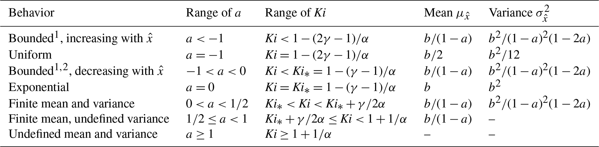
Herein we focus on rarefied motions of particles which, once entrained, travel downslope over the land surface. This notably includes the dry ravel of particles down hillslopes following disturbances (Roering and Gerber, 2005; Doane, 2018; Doane et al., 2019; Roth et al., 2020) or upon their release from obstacles (e.g., vegetation) following failure of the obstacles (Lamb et al., 2011, 2013; DiBiase and Lamb, 2013; DiBiase et al., 2017; Doane et al., 2018, 2019), and the motions of rockfall material over the surfaces of talus and scree slopes (Gerber and Scheidegger, 1974; Kirkby and Statham, 1975; Statham, 1976; Dorren, 2003; Luckman, 2013) (Fig. 1). By “rarefied motions” we are referring to the situation in which moving particles may frequently interact with the surface but rarely interact with each other. Thus, rarefied particle motions are decidedly distinct from granular flows. Indeed, processes such as rockfall and the subsequent motions of the rock material over talus or scree slopes represent the archetypal case of rarefied particle motions. Nonetheless, the ideas outlined below pertaining to the motions of individual particles may be entirely relevant to conditions that are not strictly rarefied, but where during the collective motions of many particles (e.g., during ravel) the effects of particle–surface interactions dominate over effects of particle–particle interactions in determining the behavior of the particles – akin to granular shear flows at high Knudsen number (Risso and Cordero, 2002; Kumaran, 2005, 2006). To be clear, the Knudsen number Kn is conventionally defined as the ratio of the mean free path between particle–particle collisions and a characteristic length, for example, a system dimension, a gradient length scale, or a numerical resolution scale; also see Sect. 2 in Furbish et al. (2018b). (For an ordinary gas, the onset of rarefied conditions occurs when Kn≳0.01.) We note that laboratory experiments (Kirkby and Statham, 1975; Gabet and Mendoza, 2012; Furbish et al., 2021a) and field-based experiments (DiBiase et al., 2017; Roth et al., 2020) designed to mimic particle motions and travel distances on hillslopes effectively focus on rarefied conditions. Indeed, these conditions represent one of the most fundamental of Earth surface processes imaginable – how individual sediment particles that are not transported by a fluid move down a rough inclined surface.

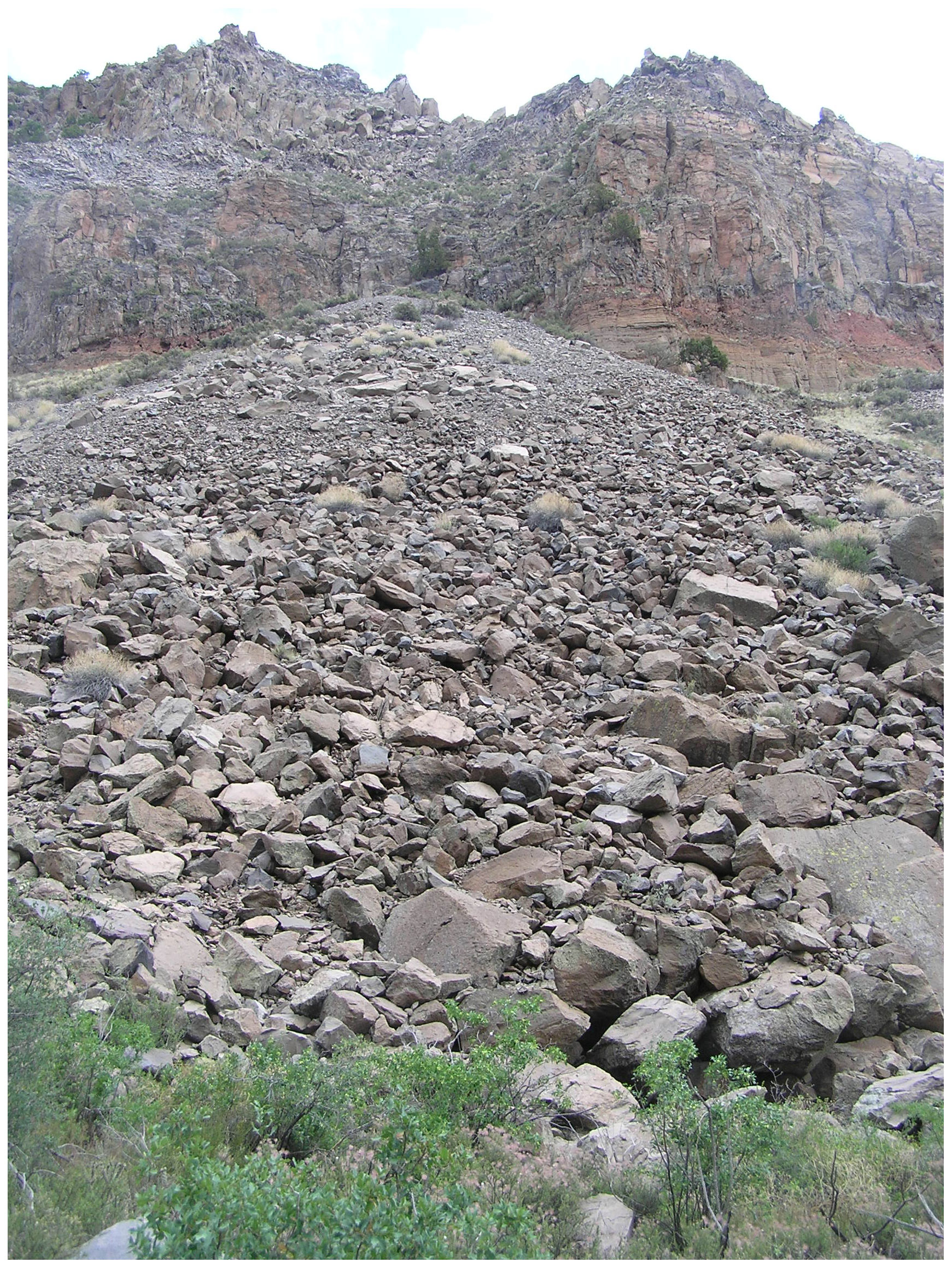
Figure 1 Image of talus slope at the base of cliffs of the Bandelier Tuff showing downslope sorting of particle sizes, with the largest particles preferentially accumulating near the base of the slope. The largest boulders in the foreground are about 1 m in diameter. As described in the text, we suspect that with conversion of translational to rotational kinetic energy, large spinning particles are less likely to be stopped by collisional friction than are small or angular particles for the same surface roughness, thus contributing to the sorting in this image. Image location is at the confluence of the Rito de los Frijoles river canyon with the Rio Grande river canyon on the eastern boundary of the Bandelier National Monument, New Mexico, USA.

The purpose of this paper is to provide a probabilistic description of the physics of rarefied particle motions and disentrainment. This involves threading together elements of statistical mechanics, concepts from granular gas theory, particle collision mechanics, and probability distribution theory. To motivate the formalism we start in Sect. 2 with a probabilistic definition of the particle disentrainment rate and show its relation to the entrainment forms of the flux and the Exner equation, following previous presentations (Furbish and Haff, 2010; Furbish and Roering, 2013). This highlights how the disentrainment rate determines the probability distribution of travel distances and thus connects descriptions of the flux and mass conservation with the physics of particle motions. In Sect. 3 we formulate disentrainment in terms of particle energetics, where the particles are treated as a rarefied granular gas. Ensemble-averaged motions are described in terms of a balance between gravitational heating and frictional cooling, wherein the latter leads to deposition. We neglect entrainment. (Our choice of terminology is based on that of granular physics as outlined in Appendix A.) The analysis in Sect. 4 illustrates the effects of collisional friction in determining the basic form of the distribution of travel distances, a generalized Pareto distribution. Depending on the balance between heating and cooling, this distribution transitions from a bounded form representing rapid thermal collapse to a heavy-tailed form representing net particle heating. In Sect. 5 we compare the formulation with previous descriptions of disentrainment, showing both similarities and dissimilarities with these descriptions. These include the formulation of Kirkby and Statham (1975), which involves a particle energy balance assuming a Coulomb-like friction behavior, and the formulation of Gabet and Mendoza (2012), which starts with a particle momentum balance involving gravity, Coulomb friction and collisional friction. We then consider elements of the probabilistic formulation presented by Furbish and Haff (2010), Furbish and Roering (2013), and Doane et al. (2018), which assumes a fixed disentrainment rate determined by the local surface slope for given surface roughness.

We emphasize that this initial phase of our work on rarefied particle motions is aimed at clarifying how particle disentrainment works. With this in place we will be positioned to consider effects of rarefied transport over timescales spanning many transport events, including ensemble-averaged particle fluxes and changes in land-surface elevation as described by formulations of nonlocal transport. As a step in this effort we show in the second companion paper (Furbish et al., 2021a) that the theory in this first paper is entirely consistent with data from laboratory and field-based experiments involving measurements of particle travel distances on rough surfaces. These include data reported by Kirkby and Statham (1975), Gabet and Mendoza (2012), DiBiase et al. (2017), and Roth et al. (2020) and new travel distance data from laboratory experiments supplemented with high-speed imaging and audio recordings that highlight effects of particle–surface collisions. Outstanding questions concern how particle size and shape in concert with surface roughness influence the extraction of particle energy and the likelihood of deposition.

In the third companion paper (Furbish et al., 2021b) we show that the generalized Pareto distribution in this problem is a maximum entropy distribution (Jaynes, 1957a, b) constrained by a fixed energetic “cost” – the total cumulative energy extracted by collisional friction per unit kinetic energy available during particle motions. That is, among all possible accessible microstates – the many different ways to arrange a great number of particles into distance states where each arrangement satisfies the same fixed total energetic cost – the generalized Pareto distribution represents the most probable arrangement. Because this idea applies equally to the accessible microstates associated with net cooling, isothermal conditions and net heating, the fixed energetic cost provides a unifying interpretation for these distinctive behaviors, including the abrupt transition in the form of the generalized Pareto distribution in crossing isothermal conditions. The analysis therefore represents a novel generalization of an energy-based constraint in using the maximum entropy method to infer non-exponential distributions of particle motions.

In the fourth companion paper (Furbish and Doane, 2021) we step back and examine the philosophical underpinning of the statistical mechanics framework for describing sediment particle motions and transport. Specifically, the analyses presented in the first three companion papers provide an ideal case study for highlighting three key elements of this framework: the merits of probabilistic versus deterministic descriptions of sediment motions; the implications of rarefied versus continuum transport conditions; and the consequences of increasing uncertainty in descriptions of sediment motions and transport that accompany increasing length scales and timescales. We use the analyses to illustrate the mechanistic yet probabilistic nature of the approach, highlighting the idea that the endeavor is not simply about adopting theory or methods of statistical mechanics “off the shelf” but rather involves appealing to the style of thinking of statistical mechanics while tailoring the analysis to the process and scale of interest. Under rarefied transport conditions, descriptions of the particle flux and its divergence pertain to ensemble conditions involving a distribution of possible outcomes, each realization being compatible with the controlling factors. When these factors change over time, individual outcomes reflect a legacy of earlier conditions that depends on the rate of change in the controlling factors relative to the intermittency of particle motions. The implication is that landform configurations and associated particle fluxes reflect an inherent variability (“weather”) that is just as important as the expected (“climate”) conditions in characterizing system behavior.

2 Disentrainment rate

2.1 Continuous form

Following the presentations of Furbish and Haff (2010) and Furbish and Roering (2013), let f_r(r;x) denote the probability density function of particle travel distances r whose motions begin at position x. By definition the cumulative distribution function is

$$\begin{array}{}\text{(1)}& F_r(r;x)=\underset{\mathrm{0}}{\overset{r}{\int }}{f}_r(r^{\prime };x)\mathrm{d}{r}^{\prime },\end{array}$$

where the prime denotes a variable of integration. In turn, the exceedance probability, also referred to as the survival function, is

$$\begin{array}{}\text{(2)}& R_r(r;x)=\mathrm{1}-F_r(r;x)=\underset{r}{\overset{\mathrm{\infty }}{\int }}{f}_r(r^{\prime };x)\mathrm{d}{r}^{\prime }.\end{array}$$

With these definitions in place we now define the spatial disentrainment rate as

$$\begin{array}{}\text{(3)}& P_r(r;x)={\displaystyle \frac{f_r(r;x)}{\mathrm{1}-F_r(r;x)}}={\displaystyle \frac{f_r(r;x)}{R_r(r;x)}},\end{array}$$

which is a conditional probability per unit distance. Namely, upon multiplying both sides of Eq. (3) by dr, then $P_r(r;x)\mathrm{d}r=f_r(r;x)\mathrm{d}r/R_r(r;x)$ is interpreted as the probability that a particle will become disentrained within the small interval r to r+dr, given that it “survived” travel to the distance r. The disentrainment rate P_r(r;x) also may be interpreted as an inhomogeneous Poisson rate (Feller, 1949). Now, using the fact that $f_r(r;x)=-\mathrm{d}{R}_r(r;x)/\mathrm{d}r$, one may deduce from Eq. (3) that the probability density f_r(r;x) is given by

$$\begin{array}{}\text{(4)}& f_r(r;x)=P_r(r;x)e^{-{\int }_{\mathrm{0}}^r{P}_r(r^{\prime };x)\mathrm{d}{r}^{\prime }}.\end{array}$$

Thus, according to Eq. (4), the disentrainment rate P_r(r;x) completely determines the probability density f_r(r;x) of travel distances r.

Assuming particle motions occur only in the positive x direction, the entrainment form of the volumetric particle flux is

$$\begin{array}{}\text{(5)}& q\left(x\right)=\underset{-\mathrm{\infty }}{\overset{x}{\int }}{E}_{\mathrm{s}}\left(x^{\prime }\right)R_r(x-x^{\prime };x^{\prime })\mathrm{d}{x}^{\prime },\end{array}$$

where E_s(x) denotes the volumetric entrainment rate at position x. In turn, letting ζ(x,t) denote the local land-surface elevation, the entrainment form of the Exner equation is (Tsujimoto, 1978; Nakagawa and Tsujiomoto, 1980)

$$\begin{array}{}\text{(6)}& c_{\mathrm{s}}{\displaystyle \frac{\partial \mathit{\zeta }(x,t)}{\partial t}}=-E_{\mathrm{s}}\left(x\right)+\underset{-\mathrm{\infty }}{\overset{x}{\int }}{E}_{\mathrm{s}}\left(x^{\prime }\right)f_r(x-x^{\prime };x^{\prime })\mathrm{d}{x}^{\prime },\end{array}$$

where $c_{\mathrm{s}}=\mathrm{1}-{\mathit{\varphi }}_{\mathrm{s}}$ is the particle volumetric concentration of the surface with porosity ϕ_s. These probabilistic formulations of the flux and the Exner equation have three lovely properties. They are mass conserving, they are nonlocal in form, and they are scale independent in that no length constraints are imposed on the density f_r(r;x) (Furbish and Haff, 2010; Furbish and Roering, 2013). They illustrate that the probability density f_r(r;x) of particle travel distances r and its related survival function R_r(r;x) form the centerpiece of describing mass conservation and the particle flux. In turn, the significance of the disentrainment rate P_r(r;x) becomes clear. This rate connects Eqs. (5) and (6) to the physics of particle motions on a hillslope. That is, this rate, together with the entrainment rate E_s(x), represents the elements in the formulation that can be elucidated by physics.

To date, previous formulations of the disentrainment rate P_r(r;x) have envisioned a friction-dominated behavior in which the land-surface slope $S\left(x\right)=|\partial \mathit{\zeta }(x)/\partial x|$ has a primary role (Furbish and Haff, 2010; Furbish and Roering, 2013; Doane, 2018; Doane et al., 2018; Sect. 5.3). The disentrainment rate is specified as a function of the land-surface slope at the position of entrainment, with the idea that the slope changes over a distance much larger than the average particle travel distance. That is, P_r(r;x) is assumed to be fixed and determined locally by the slope S(x) at position x such that the distribution of travel distances of particles entrained at x is exponential with mean μ_r[S(x)]. As the land-surface slope S varies with increasing downslope distance x, the mean μ_r[S(x)] changes. The disentrainment rate is qualitatively consistent with limiting cases; namely, it yields a fixed small average travel distance at zero slope, and it approaches zero in the limit of a steep critical slope beyond which disentrainment does not occur. However, the mechanical elements of the disentrainment rate P_r(r;) are otherwise not explicitly specified. We also note that Kirkby and Statham (1975) first pointed out the relation between the distribution of travel distances and the disentrainment rate function. These authors defined a posteriori the disentrainment rate from an assumed exponential distribution of travel distances whose mean value is expressed in terms of a Coulomb-like description of particle friction (Sect. 5.1).

2.2 Discrete form

It is valuable to recast the ideas of disentrainment above in discrete form. The motivation is this. Instead of trying to formulate a continuous disentrainment rate function that is generally applicable to the entirety of a hillslope, we instead break it into discrete spatial intervals, where certain physics may be more or less important in some intervals than in others. This gets us closer to the physical ingredients of disentrainment that are occurring at different locations on a hillslope, where the mechanical behavior at a location transitions to another behavior in the downslope direction. We may then combine the intervals together as a whole.

Let $k=\mathrm{1},\mathrm{2},\mathrm{3},\mathrm{\dots }$ denote a set of discrete intervals of length dr. Let p denote the probability that a particle is disentrained within the first interval (k=1). If N denotes a great number of particles, then the number of particles n(1) disentrained within the first interval is n(1)=Np. Because $q=\mathrm{1}-p$ is the probability that a particle is not disentrained within the first interval, then the number of particles moving beyond the first interval is $Nq=N(\mathrm{1}-p)$. That is, this is the number of particles that “survived” without being disentrained within the first interval. In turn, of the number of particles that survived, the number that is disentrained within the second interval is $n\left(\mathrm{2}\right)=N(\mathrm{1}-p)p$. More generally, $n\left(k\right)=N(\mathrm{1}-p{)}^{k-\mathrm{1}}p$. Dividing this by N then gives the probability mass function

$$\begin{array}{}\text{(7)}& f_k\left(k\right)=(\mathrm{1}-p{)}^{k-\mathrm{1}}p=q^{k-\mathrm{1}}p,\end{array}$$

which defines the well-known geometric distribution with mean ${\mathit{\mu }}_k=\mathrm{1}/p$. Note that the probability p is taken here as being fixed. That is, in this formulation, the probability that a particle survives the kth interval is $(\mathrm{1}-p{)}^{k-\mathrm{1}}$, so the disentrainment probability is constant, namely, P_k(k)=p.

The geometric distribution, Eq. (7), is the discrete counterpart of the exponential distribution. Here we relate the two. The cumulative distribution function of Eq. (7) is $F_k\left(k\right)=\mathrm{1}-(\mathrm{1}-p{)}^k$. We may thus write $F_r(r=k\mathrm{d}r)=F_k\left(k\right)=\mathrm{1}-q^k$. The quantity q^k is a memoryless geometric series, and because q≤1 we may write $q=e^{-\mathrm{d}r/{\mathit{\mu }}_r}$, where μ_r is a characteristic distance. In turn, then, $F_r\left(r\right)=\mathrm{1}-(e^{-\mathrm{d}r/{\mathit{\mu }}_r}{)}^k=\mathrm{1}-e^{-r/{\mathit{\mu }}_r}$. Finally, $f_r\left(r\right)=\mathrm{d}{F}_r\left(r\right)/\mathrm{d}r=(\mathrm{1}/{\mathit{\mu }}_r)e^{-r/{\mathit{\mu }}_r}$, where it becomes clear that μ_r is the mean of the exponential distribution, analogous to μ_k for the discrete counterpart. Also note that the disentrainment rate $P_r\left(r\right)=\mathrm{1}/{\mathit{\mu }}_r$ is fixed. Below we show that the exponential and geometrical distributions represent isothermal conditions, where gravitational heating of particles is balanced by frictional cooling.

In contrast, suppose that the probability of disentrainment p varies from one interval k to another. Here we generalize the ideas above. Let p_k denote the probability that a particle, having not been disentrained before the kth interval, then becomes disentrained within this interval. Similar to the formulation above, the number of particles n(1) within the first interval is n(1)=Np₁ and the number moving beyond the first interval is N(1−p₁). In turn the number of particles disentrained within the second interval is $n\left(\mathrm{2}\right)=N(\mathrm{1}-p_{\mathrm{1}})p_{\mathrm{2}}$, the number disentrained within the third interval is $N(\mathrm{1}-p_{\mathrm{1}})(\mathrm{1}-p_{\mathrm{2}})p_{\mathrm{3}}$, and so on. In general, $n\left(k\right)=N(\mathrm{1}-p_{\mathrm{1}})(\mathrm{1}-p_{\mathrm{2}})(\mathrm{1}-p_{\mathrm{3}})\mathrm{\dots }(\mathrm{1}-p_{k-\mathrm{1}})p_k$. Dividing this expression by N then gives

$$\begin{array}{}\text{(8)}& f_k\left(k\right)=p_k\prod _{i=\mathrm{1}}^{k-\mathrm{1}}\left(\mathrm{1}-p_i\right).\end{array}$$

Note that if p_k=p is fixed, then Eq. (8) reduces to Eq. (7).

This generalization has a lovely property. Namely, by definition it conserves probability, and it therefore is mass conserving. That is, the sum of f_k(k) over all possible k is equal to unity, regardless of how p_k might vary with k. As alluded to above, the physics of each p_k may be treated differently if desired. Moreover, like its continuous counterpart presented above, this discrete formulation of mass conservation is nonlocal and scale independent.

2.3 Brief preview

Our next objective is to illustrate the mechanical elements of disentrainment, which we then use to elaborate the continuous and discrete cases described in the preceding sections. The main ingredients of the theoretical analysis involve the particle mass balance and the particle kinetic energy balance. Let N denote a great number of particles whose motions started at position x=0 such that the particle travel distance r→x. We then show that the particle mass balance is given by $\mathrm{d}N\left(x\right)/\mathrm{d}x\sim -N/E_{\mathrm{a}}$, where E_a is the ensemble-averaged kinetic energy of moving particles. In turn we show that for a uniform slope angle and surface roughness the average energy varies as $E_{\mathrm{a}}\sim Ax+B$, where A and B are the shape and scale parameters of the generalized Pareto distribution. These parameters are related to particle and surface conditions (e.g., particle size and shape, surface slope and roughness) and the initial particle energy state at x=0. We then show that the disentrainment rate $P_x\left(x\right)=-(\mathrm{1}/N)\mathrm{d}N/\mathrm{d}x=\mathrm{1}/(Ax+B)$, which, using Eq. (4), leads to the generalized Pareto distribution. When A<0, this distribution is bounded; when A>0, it is heavy-tailed; and when A=0 such that $P_x=\mathrm{1}/B$ is a fixed value, the distribution reduces to an exponential form. Deposition is an inhomogeneous Poisson process for A≠0 and it is homogeneous for A=0. We also illustrate the discrete counterpart to these results, as outlined in Sect. 2.2, including the situation of nonuniform surface conditions.

3 Mechanical interpretation of disentrainment

3.1 Conservation of mass

Consider a rough, inclined surface with uniform slope angle θ (Fig. 2). At this juncture we simplify the notation and consider the motions of particles entrained at a single position x=0. Now the particle travel distance r→x and the probability density function $f_r(r;x)\to f_x\left(x\right)$. Consider a control volume with edge length dx parallel to the mean particle motion. Over a period of time a great number of particles enter the left face of the control volume. Some of these particles move entirely through the volume, exiting its right face, and some come to rest within the control volume. Many, but not necessarily all, of the particles interact with the surface one or more times in moving through the volume or in being disentrained within it.

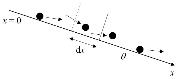
Figure 2 Definition diagram of surface inclined at angle θ and control volume with edge length dx through which particles move.

We now imagine collecting this great number of particles and treating them as a cohort, independent of time (Appendix B). That is, let N(x) denote the number of particles that enter the control volume, and let N(x+dx) denote the number that leaves the volume. We may imagine for the purpose of visualizing the problem that the N(x) particles enter the control volume at the same time, but this actually is not essential. Similarly, we may imagine that the N(x+dx) particles exit the control volume at approximately the same time, but again, this reference to time only is a means to envision particle motions (Appendix B). The number of particles disentrained within the control volume then is $\mathrm{d}N=N(x+\mathrm{d}x)-N\left(x\right)$.

If N(0) denotes the great number of particles whose motions started at position x=0, then the exceedance probability R_x(x) (analogous to R_r(r;x) above) is $R_x\left(x\right)=N\left(x\right)/N\left(\mathrm{0}\right)$. Then $\mathrm{d}N=-N\left(\mathrm{0}\right)f_x\left(x\right)\mathrm{d}x$ and the spatial disentrainment rate P_x(x) (analogous to P_r(r) above) is

$$\begin{array}{}\text{(9)}& P_x\left(x\right)=-{\displaystyle \frac{\mathrm{1}}{N\left(x\right)}}{\displaystyle \frac{\mathrm{d}N\left(x\right)}{\mathrm{d}x}}.\end{array}$$

Our objective is to determine the derivative $\mathrm{d}N\left(x\right)/\mathrm{d}$ in relation to particle energy, as this derivative represents disentrainment. Here we summarize the essence of this problem before turning to a description of conservation of energy.

Let $E_{\mathrm{p}}=(m/\mathrm{2})u^{\mathrm{2}}$ denote the translational kinetic energy of a particle with mass m and downslope velocity u. Here we are assuming that the total translational energy is dominated by downslope motion. Let $f_{E_{\mathrm{p}}}(E_{\mathrm{p}},x)$ denote the probability density function of particle energies E_p as these vary with position x. For a great number N of particles the number density is $n_{E_{\mathrm{p}}}(E_{\mathrm{p}},x)=N{f}_{E_{\mathrm{p}}}(E_{\mathrm{p}},x)$. Let p(E_p,x) denote the probability that a particle at energy state E_p will become disentrained within the small interval x to x+dx. Because $N{f}_{E_{\mathrm{p}}}(E_{\mathrm{p}},x)\mathrm{d}{E}_{\mathrm{p}}$ is the number of particles within the small interval E_p to E_p+dE_p, then $Np(E_{\mathrm{p}},x)f_{E_{\mathrm{p}}}(E_{\mathrm{p}},x)\mathrm{d}{E}_{\mathrm{p}}$ is the number of particles in this energy interval that becomes disentrained. The total number of particles that becomes disentrained within the interval x to x+dx is then

$$\begin{array}{}\text{(10)}& \mathrm{d}N\left(x\right)=-N\left(x\right)\underset{\mathrm{0}}{\overset{\mathrm{\infty }}{\int }}p\left(E_{\mathrm{p}},x\right)f_{E_{\mathrm{p}}}\left(E_{\mathrm{p}},x\right)\mathrm{d}{E}_{\mathrm{p}}.\end{array}$$

Letting angle brackets denote an ensemble average, then according to the law of the unconscious statistician, Eq. (10) is simply $\mathrm{d}N\left(x\right)=-N\left(x\right)\langle p(E_{\mathrm{p}},x)\rangle$. Below we introduce the expected number of particle–surface collisions per unit distance $n_x=\mathrm{1}/\mathit{\lambda }$, where λ is the expected travel distance between successive collisions. We then show that $\mathrm{d}N\left(x\right)/\mathrm{d}x=-N\left(x\right)n_x\langle p(E_{\mathrm{p}},x)\rangle$. Thus, the essence of the problem is to determine the averaged probability 〈p(E_p,x)〉 as this depends on particle energy E_p. This in turn requires specifying the particle energy as this varies with position x.

3.2 Particle energy

Our focus on conservation of particle energy versus momentum is aimed at defensible simplicity. Namely, particle motions down a rough hillslope surface involve numerous details that control momentum exchanges during particle–surface interactions. As a scalar quantity, energy forces us to blur our eyes appropriately, focusing on the essence of these complex interactions rather than attempting to describe details of momentum exchanges that ultimately cannot be constrained given the stochastic nature of the phenomenon. As an example, below we introduce the random variable β_x to represent the proportion of downslope kinetic energy extracted during a particle–surface collision. This quantity blurs over many details (e.g., differences between collisions during rolling, tumbling and bouncing motions, rotational versus translational motion, and the roles of normal and tangential coefficients of restitution), yet β_x is entirely meaningful when treated as a random variable. (In Appendix E we provide a description of how the energy-centric quantity β_x is related to momentum exchanges during collisions, and in the companion paper we illustrate the elements of β_x using high-speed imaging.) In contrast, when describing the collisional behavior of an ideal granular gas, one can at lowest order appeal to a single coefficient of restitution because of the relative simplicity of the particles and their collisions (e.g., Haff, 1983; Jenkins and Savage, 1983). This simplicity is not possible here. The focus on energy thus offers tractable and defensible simplicity amidst the messiness of natural hillslopes.

We start our formulation with a general statement concerning conservation of the kinetic energy of a system of particles. Because of its familiarity in relation to studies of granular gas systems, we initially consider changes with respect to time, then return to changes with respect to space as in the preceding section. Namely, let E_p denote the kinetic energy of a particle, and let 〈E_p〉 denote the expected energy state, where angle brackets represent an ensemble average over a great number N of moving particles. The total energy of the system is E=N〈E_p〉. Neglecting transport of energy over space, the rate of change in the total energy of the system with respect to time is then

$$\begin{array}{}\text{(11)}& {\displaystyle \frac{\mathrm{d}E}{\mathrm{d}t}}=N{\displaystyle \frac{\mathrm{d}\langle E_{\mathrm{p}}\rangle }{\mathrm{d}t}}+\langle E_{\mathrm{p}}\rangle {\displaystyle \frac{\mathrm{d}N}{\mathrm{d}t}}.\end{array}$$

The first term on the right side of Eq. (11) represents the rate of change in the average energy state of N moving particles and thus describes either a net heating ($\mathrm{d}\langle E_{\mathrm{p}}\rangle /\mathrm{d}t>\mathrm{0}$) or cooling ($\mathrm{d}\langle E_{\mathrm{p}}\rangle /\mathrm{d}t<\mathrm{0}$) of the system, depending on the relative contribution of the sources of each. The second term on the right side represents the rate of change in the number of moving particles with average energy state 〈E_p〉 and thus describes the rate of change in the total energy due to either the addition or loss of moving particles. For a closed system, this represents either a net sublimation ($\mathrm{d}N/\mathrm{d}t>\mathrm{0}$) or net deposition ($\mathrm{d}N/\mathrm{d}t<\mathrm{0}$) of particles, depending on the relative contribution of each.

The first term on the right side of Eq. (11) has been studied extensively for granular gas systems, specifically in relation to the “homogeneous cooling state” of a closed system as described by Haff's cooling law (Haff, 1983; Brilliantov and Pöschel, 2004; Dominguez and Zenit, 2007; Volfson et al., 2007; Brilliantov et al., 2018; Yu et al., 2020). In what follows, we start with similar concepts of particle energy, but the formulation is designed to be independent of time and focused on changes in energy and particle disentrainment over space.

Reconsider a control volume with edge length dx parallel to the mean motion of particles over a rough, inclined surface (Fig. 2). Analogous to Eq. (11) we write

$$\begin{array}{}\text{(12)}& {\displaystyle \frac{\mathrm{d}E}{\mathrm{d}x}}=N{\displaystyle \frac{\mathrm{d}\langle E_{\mathrm{p}}\rangle }{\mathrm{d}x}}+\langle E_{\mathrm{p}}\rangle {\displaystyle \frac{\mathrm{d}N}{\mathrm{d}x}},\end{array}$$

where now the angle brackets formally denote a Gibbs ensemble average over a cohort of particles (Appendix B). As described below, the first term on the right side of Eq. (12) represents the spatial rate of change in energy due to the sum of gravitational heating and frictional cooling. The second term on the right side represents the rate of change in energy due to deposition, that is, disentrainment. In this problem, we assume that sublimation (entrainment) does not occur over x>0. Equation (12) provides a basic starting point. However, it is not particularly useful in this form. If in fact the probability of deposition varies with energy state, then in general the derivative $\mathrm{d}N/\mathrm{d}x$ contributes to the derivative $\mathrm{d}\langle E_{\mathrm{p}}\rangle /\mathrm{d}x$, as removal of energy by deposition affects the average energy of the remaining particles. We note that Brilliantov et al. (2018) demonstrate an analogous effect, as described below, associated with aggregation of particles in a granular gas. We therefore must be careful in formulating a statement of conservation of particle energy, as deposition preferentially involves particles at low-energy states.

3.3 Conservation of energy

3.3.1 Total energy

Focusing just on slope parallel motions, let $E_{\mathrm{p}}=(m/\mathrm{2})u^{\mathrm{2}}$ denote the translational kinetic energy of a particle with mass m and downslope velocity u. Then let $f_{E_{\mathrm{p}}}(E_{\mathrm{p}},x)$ denote the probability density function of particle energies E_p as these vary with downslope position x (Appendix B). For a great number N of particles the number density is $n_{E_{\mathrm{p}}}(E_{\mathrm{p}},x)=N{f}_{E_{\mathrm{p}}}(E_{\mathrm{p}},x)$. The average particle energy is

$$\begin{array}{}\text{(13)}& \begin{array}{rl}\langle E_{\mathrm{p}}\rangle & =\underset{\mathrm{0}}{\overset{\mathrm{\infty }}{\int }}{E}_{\mathrm{p}}{f}_{E_{\mathrm{p}}}\left(E_{\mathrm{p}},x\right)\mathrm{d}{E}_{\mathrm{p}}\\ & ={\displaystyle \frac{\mathrm{1}}{N}}\underset{\mathrm{0}}{\overset{\mathrm{\infty }}{\int }}{E}_{\mathrm{p}}{n}_{E_{\mathrm{p}}}\left(E_{\mathrm{p}},x\right)\mathrm{d}{E}_{\mathrm{p}}.\end{array}\end{array}$$

The total energy E(x)=N〈E_p〉, so

$$\begin{array}{}\text{(14)}& E\left(x\right)=\underset{\mathrm{0}}{\overset{\mathrm{\infty }}{\int }}{E}_{\mathrm{p}}{n}_{E_{\mathrm{p}}}\left(E_{\mathrm{p}},x\right)\mathrm{d}{E}_{\mathrm{p}}.\end{array}$$

We now take the derivative of Eq. (14) with respect to x using Leibniz's rule to give

$$\begin{array}{}\text{(15)}& {\displaystyle \frac{\mathrm{d}E\left(x\right)}{\mathrm{d}x}}=\underset{\mathrm{0}}{\overset{\mathrm{\infty }}{\int }}{E}_{\mathrm{p}}{\displaystyle \frac{\partial n_{E_{\mathrm{p}}}\left(E_{\mathrm{p}},x\right)}{\partial x}}\mathrm{d}{E}_{\mathrm{p}}.\end{array}$$

The derivative within the integral of Eq. (15) satisfies a Fokker–Planck equation (see next section and Appendix C), the solution of which represents the evolution of the distribution $n_{E_{\mathrm{p}}}(E_{\mathrm{p}},x)$ of particle energy states E_p with distance x. In particular this derivative has three parts. The first part, denoted below by K_h(E_p,x), is associated with a change in the density $n_{E_{\mathrm{p}}}(E_{\mathrm{p}},x)$ due to gravitational heating. The second part, K_c(E_p,x), is associated with a change in this density due to frictional cooling. The third part, K_d(E_p,x), is associated with a loss of energy due to deposition (which does not involve the analogue of release of latent heat; but see below). We thus write

$$\begin{array}{}\text{(16)}& {\displaystyle \frac{\partial n_{E_{\mathrm{p}}}\left(E_{\mathrm{p}},x\right)}{\partial x}}=K_{\mathrm{h}}\left(E_{\mathrm{p}},x\right)+K_{\mathrm{c}}\left(E_{\mathrm{p}},x\right)+K_{\mathrm{d}}\left(E_{\mathrm{p}},x\right),\end{array}$$

and then rewrite Eq. (15) as

$$\begin{array}{}\text{(17)}& \begin{array}{rl}{\displaystyle \frac{\mathrm{d}E\left(x\right)}{\mathrm{d}x}}& =\underset{\mathrm{0}}{\overset{\mathrm{\infty }}{\int }}{E}_{\mathrm{p}}{K}_{\mathrm{h}}\left(E_{\mathrm{p}},x\right)\mathrm{d}{E}_{\mathrm{p}}\\ & +\underset{\mathrm{0}}{\overset{\mathrm{\infty }}{\int }}{E}_{\mathrm{p}}{K}_{\mathrm{c}}\left(E_{\mathrm{p}},x\right)\mathrm{d}{E}_{\mathrm{p}}\\ & +\underset{\mathrm{0}}{\overset{\mathrm{\infty }}{\int }}{E}_{\mathrm{p}}{K}_{\mathrm{d}}\left(E_{\mathrm{p}},x\right)\mathrm{d}{E}_{\mathrm{p}}.\end{array}\end{array}$$

The next task consists of showing the correspondence of K_h(E_p,x), K_c(E_p,x) and K_d(E_p,x) to terms in the Fokker–Planck equation, then describing the physical elements of these terms. This is followed by evaluating each of the integral quantities in Eq. (17). There are a lot of moving parts in this formulation, so bear with us.

3.3.2 Fokker–Planck-like equation

The density $n_{E_{\mathrm{p}}}(E_{\mathrm{p}},x)$ within Eqs. (15) and (16) satisfies a Fokker–Planck equation (Appendix C), which describes the evolution of this density with increasing distance x. Namely,

$$\begin{array}{}\text{(18)}& \begin{array}{rl}{\displaystyle \frac{\partial n_{E_{\mathrm{p}}}\left(E_{\mathrm{p}},x\right)}{\partial x}}& =-{\displaystyle \frac{\partial }{\partial E_{\mathrm{p}}}}\left[k_{\mathrm{1}\mathrm{h}}\left(E_{\mathrm{p}},x\right)n_{E_{\mathrm{p}}}\left(E_{\mathrm{p}},x\right)\right]\\ & -{\displaystyle \frac{\partial }{\partial E_{\mathrm{p}}}}\left[k_{\mathrm{1}\mathrm{c}}\left(E_{\mathrm{p}},x\right)n_{E_{\mathrm{p}}}\left(E_{\mathrm{p}},x\right)\right]\\ & +{\displaystyle \frac{\mathrm{1}}{\mathrm{2}}}{\displaystyle \frac{{\partial }^{\mathrm{2}}}{\partial E_{\mathrm{p}}^{\mathrm{2}}}}\left[k_{\mathrm{2}\mathrm{c}}\left(E_{\mathrm{p}},x\right)n_{E_{\mathrm{p}}}\left(E_{\mathrm{p}},x\right)\right]\\ & -K_{\mathrm{d}}\left(E_{\mathrm{p}},x\right).\end{array}\end{array}$$

The first term on the right side of Eq. (18) represents advective gravitational heating, where k_1h(E_p,x) is a drift speed, the average spatial rate of change in particle energy over the energy domain due to heating. The second term on the right side represents advective frictional cooling, where k_1c(E_p,x) is a drift speed, the average spatial rate of change in particle energy due to cooling. The third term represents diffusive frictional cooling, where k_2c(E_p,x) is a diffusion coefficient. The last term represents a loss of energy due to deposition, where for now we have retained the notation from above. Explicitly, for K_h(E_p,x) and K_c(E_p,x) we now have

$$\begin{array}{}\text{(19)}& K_{\mathrm{h}}\left(E_{\mathrm{p}},x\right)=-{\displaystyle \frac{\partial }{\partial E_{\mathrm{p}}}}\left[k_{\mathrm{1}\mathrm{h}}\left(E_{\mathrm{p}},x\right)n_{E_{\mathrm{p}}}\left(E_{\mathrm{p}},x\right)\right]\end{array}$$

and

$$\begin{array}{}\text{(20)}& \begin{array}{rl}{K}_{\mathrm{c}}\left(E_{\mathrm{p}},x\right)& =-{\displaystyle \frac{\partial }{\partial E_{\mathrm{p}}}}\left[k_{\mathrm{1}\mathrm{c}}\left(E_{\mathrm{p}},x\right)n_{E_{\mathrm{p}}}\left(E_{\mathrm{p}},x\right)\right]\\ & +{\displaystyle \frac{\mathrm{1}}{\mathrm{2}}}{\displaystyle \frac{{\partial }^{\mathrm{2}}}{\partial E_{\mathrm{p}}^{\mathrm{2}}}}\left[k_{\mathrm{2}\mathrm{c}}\left(E_{\mathrm{p}},x\right)n_{E_{\mathrm{p}}}\left(E_{\mathrm{p}},x\right)\right].\end{array}\end{array}$$

In the next section we step through gravitational heating, frictional cooling and deposition, in each case unfolding the mechanical elements of k_1h(E_p,x), k_1c(E_p,x), k_2c(E_p,x) and K_d(E_p,x).

Here is a didactic sidebar if the formulation above seems counterintuitive. Notice that Eq. (18) effectively represents an advection–diffusion equation with two advective terms, a diffusive term and a sink term. Normally we think of an advection–diffusion equation as involving space and time, that is, where the rate at which a quantity changes with respect to time at a given position is equal to the sum of an advective term and a diffusive term involving derivatives of the quantity with respect to space. Indeed, imagine replacing E_p with x, and x with t, in Eq. (18). The result looks like a familiar advection–diffusion equation with a sink term (albeit involving two advective terms rather than one). The basic idea of Eq. (18) is the same. It just describes the rate of change in $n_{E_{\mathrm{p}}}$ with respect to position x (rather than time t) in relation to advection and diffusion of $n_{E_{\mathrm{p}}}$ occurring over the energy coordinate E_p (rather than x). A consideration of the rate of change with respect to position x as in Eq. (18) is perhaps unusual, but the idea of advection and diffusion of a quantity occurring over a domain other than a spatial coordinate (e.g., a velocity coordinate) is common in statistical physics, of which examples pertaining to sediment motions include those presented in Furbish et al. (2012, 2018a, b).

3.3.3 Gravitational heating

We start by noting that the rate at which the potential energy of a particle is converted to kinetic energy per unit distance x is mgsin θ. To be clear, between collisions a particle that is not in contact with the inclined surface beneath it accelerates vertically at a rate of −g, independently of the orientation of the surface. The factor sin θ therefore is a geometrical constraint on the magnitude of the potential energy that is accessible for net heating when viewed with respect to x. This means that (Appendix C)

$$\begin{array}{}\text{(21)}& k_{\mathrm{1}\mathrm{h}}\left(E_{\mathrm{p}},x\right)\to k_{\mathrm{1}h}=mg\sin \mathit{\theta },\end{array}$$

so that Eq. (19) becomes

$$\begin{array}{}\text{(22)}& K_{\mathrm{h}}\left(E_{\mathrm{p}},x\right)=-mg\sin \mathit{\theta }{\displaystyle \frac{\partial n_{E_{\mathrm{p}}}\left(E_{\mathrm{p}},x\right)}{\partial E_{\mathrm{p}}}}.\end{array}$$

We now write the first integral in Eq. (17) as

$$\begin{array}{}\text{(23)}& -mg\sin \mathit{\theta }\underset{\mathrm{0}}{\overset{\mathrm{\infty }}{\int }}{E}_{\mathrm{p}}{\displaystyle \frac{\partial n_{E_{\mathrm{p}}}\left(E_{\mathrm{p}},x\right)}{\partial E_{\mathrm{p}}}}\mathrm{d}{E}_{\mathrm{p}}.\end{array}$$

Because $\partial \left(E_{\mathrm{p}}{n}_{E_{\mathrm{p}}}\right)/\partial E_{\mathrm{p}}=E_{\mathrm{p}}\partial n_{E_{\mathrm{p}}}/\partial E_{\mathrm{p}}+n_{E_{\mathrm{p}}}$, Eq. (23) may be written as

$$\begin{array}{}\text{(24)}& \begin{array}{rl}mg\sin \mathit{\theta }& \underset{\mathrm{0}}{\overset{\mathrm{\infty }}{\int }}{n}_{E_{\mathrm{p}}}\left(E_{\mathrm{p}},x\right)\mathrm{d}{E}_{\mathrm{p}}\\ & -mg\sin \mathit{\theta }\underset{\mathrm{0}}{\overset{\mathrm{\infty }}{\int }}{\displaystyle \frac{\partial }{\partial E_{\mathrm{p}}}}\left[E_{\mathrm{p}}{n}_{E_{\mathrm{p}}}\left(E_{\mathrm{p}},x\right)\right]\mathrm{d}{E}_{\mathrm{p}}.\end{array}\end{array}$$

Assuming $n_{E_{\mathrm{p}}}(\mathrm{\infty },x)\to \mathrm{0}$, the second integral in Eq. (24) vanishes and the first integral in Eq. (17) becomes

$$\begin{array}{}\text{(25)}& \underset{\mathrm{0}}{\overset{\mathrm{\infty }}{\int }}{E}_{\mathrm{p}}{K}_{\mathrm{h}}\left(E_{\mathrm{p}},x\right)\mathrm{d}{E}_{\mathrm{p}}=Nmg\sin \mathit{\theta }.\end{array}$$

Note that the form of the density $n_{E_{\mathrm{p}}}(E_{\mathrm{p}},x)$ is immaterial in this formulation.

If for illustration we assume that no cooling or deposition occurs, then $\mathrm{d}E\left(x\right)/\mathrm{d}x=Nmg\sin \mathit{\theta }$. The solution of this is $E\left(x\right)=E\left(\mathrm{0}\right)+Nmg\sin \mathit{\theta }x$, where E(0) denotes the starting energy at x=0. That is, the total kinetic energy E(x) increases linearly with downslope distance x. Moreover, for reference below, no particle can be heated to an energy greater than E_p(0)+mgsin θx, representing a complete conversion of gravitational to kinetic energy without any loss due to particle–surface collisions. This ensures that the density $n_{E_{\mathrm{p}}}(E_{\mathrm{p}},x)$ is bounded with finite mean and variance, a point that becomes useful below.

3.3.4 Frictional cooling

We start by assuming that a change in the downslope energy of a particle associated with a collision is $\mathrm{\Delta }{E}_{\mathrm{p}}=-{\mathit{\beta }}_x{E}_{\mathrm{p}}$, so that ${\mathit{\beta }}_x=-\mathrm{\Delta }{E}_{\mathrm{p}}/E_{\mathrm{p}}$ is the proportion of energy extracted by the collision (Appendix E). This is akin to the dissipation factor introduced by Quartier et al. (2000). By definition β_x is a random variable. (Note that the negative sign above is by convention. As a random variable we are assuming that $\mathrm{0}\le {\mathit{\beta }}_x\le \mathrm{1}$. The sign associated with β_x will be clear from the context in the developments below.) The change ΔE_p includes frictional loss, any conversion of translational to rotational energy, and any apparent change when downslope incident motion is reflected to transverse motion during a glancing particle–surface collision. Note that ΔE_p generally is a negative quantity. But strictly speaking it could be positive, albeit with low probability, if transverse incident motion is reflected to downslope motion during a collision. Because E_p and β_x are random variables, ΔE_p is a random variable. As a point of reference, in granular gas theory where the total translational energy is considered rather than just the energy associated with one coordinate direction, the proportion ${\mathit{\beta }}_x=\mathrm{1}-{\mathit{ϵ}}^{\mathrm{2}}$ where ϵ is the normal coefficient of restitution (Haff, 1983). Normally ϵ is treated as a fixed deterministic quantity, although recent efforts have treated this quantity as a random variable (Gunkelmann et al., 2014; Serero et al., 2015). Here, in contrast, collision mechanics theory suggests that the constitution of β_x is far more complicated in relation to normal, tangential and rotational impulses during particle–surface collisions (Appendix E).

Let $q=E_{\mathrm{p}}(x+\mathrm{d}x)-E_{\mathrm{p}}\left(x\right)$ denote a change in the energy of a particle over the small distance dx. Then as described in Appendix C, the drift speed $k_{\mathrm{1}\mathrm{c}}(E_{\mathrm{p}},x)=\mathrm{d}\stackrel{\mathrm{‾}}{q}/\mathrm{d}x\approx n_x\stackrel{\mathrm{‾}}{{\mathit{\beta }}_x}{E}_{\mathrm{p}}$ and the diffusion coefficient $k_{\mathrm{2}\mathrm{c}}=\mathrm{d}\stackrel{\mathrm{‾}}{q^{\mathrm{2}}}/\mathrm{d}x\approx n_x\stackrel{\mathrm{‾}}{{\mathit{\beta }}_x^{\mathrm{2}}}{E}_{\mathrm{p}}^{\mathrm{2}}$, where the overline denotes an average over particles at the energy state E_p (rather than an ensemble average), and $n_x=\mathrm{1}/\mathit{\lambda }$ denotes the expected number of particle–surface collisions per unit distance where λ is the expected travel distance between collisions. Scaling (Appendix D) shows that

$$\begin{array}{}\text{(26)}& n_x={\displaystyle \frac{\mathrm{1}}{\mathit{\lambda }}}\approx {\displaystyle \frac{mg\cos \mathit{\theta }}{\mathrm{4}{E}_{\mathrm{p}}\tan \mathit{\varphi }}},\end{array}$$

where ϕ is the expected reflection angle of a particle with energy E_p following a surface collision. We now assume that

$$\begin{array}{}\text{(27)}& k_{\mathrm{1}\mathrm{c}}\left(E_{\mathrm{p}},x\right)\sim n_x\stackrel{\mathrm{‾}}{{\mathit{\beta }}_x}{E}_{\mathrm{p}}\approx {\displaystyle \frac{mg\stackrel{\mathrm{‾}}{{\mathit{\beta }}_x}\cos \mathit{\theta }}{\mathrm{4}\tan \mathit{\varphi }}},\end{array}$$

and that

$$\begin{array}{}\text{(28)}& k_{\mathrm{2}\mathrm{c}}\left(E_{\mathrm{p}},x\right)\sim n_x\stackrel{\mathrm{‾}}{{\mathit{\beta }}_x^{\mathrm{2}}}{E}_{\mathrm{p}}^{\mathrm{2}}\approx {\displaystyle \frac{mg\stackrel{\mathrm{‾}}{{\mathit{\beta }}_x^{\mathrm{2}}}{E}_{\mathrm{p}}\cos \mathit{\theta }}{\mathrm{4}\tan \mathit{\varphi }}}.\end{array}$$

Now Eq. (20) becomes

$$\begin{array}{}\text{(29)}& \begin{array}{rl}{K}_{\mathrm{c}}\left(E_{\mathrm{p}},x\right)& ={\displaystyle \frac{mg\cos \mathit{\theta }}{\mathrm{4}\tan \mathit{\varphi }}}{\displaystyle \frac{\partial }{\partial E_{\mathrm{p}}}}\left[\stackrel{\mathrm{‾}}{{\mathit{\beta }}_x}{n}_{E_{\mathrm{p}}}\left(E_{\mathrm{p}},x\right)\right]\\ & +{\displaystyle \frac{mg\cos \mathit{\theta }}{\mathrm{8}\tan \mathit{\varphi }}}{\displaystyle \frac{{\partial }^{\mathrm{2}}}{\partial E_{\mathrm{p}}^{\mathrm{2}}}}\left[\stackrel{\mathrm{‾}}{{\mathit{\beta }}_x^{\mathrm{2}}}{E}_{\mathrm{p}}{n}_{E_{\mathrm{p}}}\left(E_{\mathrm{p}},x\right)\right].\end{array}\end{array}$$

We now use these results to write the second integral in Eq. (17) as

$$\begin{array}{}\text{(30)}& \begin{array}{rl}{\displaystyle \frac{mg\cos \mathit{\theta }}{\mathrm{4}\tan \mathit{\varphi }}}& \underset{\mathrm{0}}{\overset{\mathrm{\infty }}{\int }}{E}_{\mathrm{p}}{\displaystyle \frac{\partial }{\partial E_{\mathrm{p}}}}\left[\stackrel{\mathrm{‾}}{{\mathit{\beta }}_x}{n}_{E_{\mathrm{p}}}\left(E_{\mathrm{p}},x\right)\right]\mathrm{d}{E}_{\mathrm{p}}\\ & +{\displaystyle \frac{mg\cos \mathit{\theta }}{\mathrm{8}\tan \mathit{\varphi }}}\underset{\mathrm{0}}{\overset{\mathrm{\infty }}{\int }}{E}_{\mathrm{p}}{\displaystyle \frac{{\partial }^{\mathrm{2}}}{\partial E_{\mathrm{p}}^{\mathrm{2}}}}\left[\stackrel{\mathrm{‾}}{{\mathit{\beta }}_x^{\mathrm{2}}}{E}_{\mathrm{p}}{n}_{E_{\mathrm{p}}}\left(E_{\mathrm{p}},x\right)\right]\mathrm{d}{E}_{\mathrm{p}}.\end{array}\end{array}$$

Upon applying the product rule to the derivative $\partial \left(E_{\mathrm{p}}\stackrel{\mathrm{‾}}{{\mathit{\beta }}_x}{n}_{E_{\mathrm{p}}}\right)/\partial E_{\mathrm{p}}$, the first integral in Eq. (30) may be written as

$$\begin{array}{}\text{(31)}& \begin{array}{rl}\underset{\mathrm{0}}{\overset{\mathrm{\infty }}{\int }}& \stackrel{\mathrm{‾}}{{\mathit{\beta }}_x}{n}_{E_{\mathrm{p}}}\left(E_{\mathrm{p}},x\right)\mathrm{d}{E}_{\mathrm{p}}\\ & -\underset{\mathrm{0}}{\overset{\mathrm{\infty }}{\int }}{\displaystyle \frac{\partial }{\partial E_{\mathrm{p}}}}\left[E_{\mathrm{p}}\stackrel{\mathrm{‾}}{{\mathit{\beta }}_x}{n}_{E_{\mathrm{p}}}\left(E_{\mathrm{p}},x\right)\right]\mathrm{d}{E}_{\mathrm{p}}.\end{array}\end{array}$$

Assuming that $n_{E_{\mathrm{p}}}(\mathrm{\infty },x)\to \mathrm{0}$, the second integral in Eq. (31) vanishes and the first integral becomes N〈β_x〉, where the angle brackets now represent an ensemble average.

In turn, upon applying the product rule to the derivative $\partial [E_{\mathrm{p}}\partial (\stackrel{\mathrm{‾}}{{\mathit{\beta }}_x^{\mathrm{2}}}{E}_{\mathrm{p}}{n}_{E_{\mathrm{p}}})/\partial E_{\mathrm{p}}]/\partial E_{\mathrm{p}}$, the second integral in Eq. (30) may be written as

$$\begin{array}{}\text{(32)}& \begin{array}{rl}{\displaystyle \frac{mg\cos \mathit{\theta }}{\mathrm{8}\tan \mathit{\varphi }}}& \underset{\mathrm{0}}{\overset{\mathrm{\infty }}{\int }}{\displaystyle \frac{\partial }{\partial E_{\mathrm{p}}}}\left(E_{\mathrm{p}}{\displaystyle \frac{\partial }{\partial E_{\mathrm{p}}}}\left[\stackrel{\mathrm{‾}}{{\mathit{\beta }}_x^{\mathrm{2}}}{E}_{\mathrm{p}}{n}_{E_{\mathrm{p}}}\left(E_{\mathrm{p}},x\right)\right]\right)\mathrm{d}{E}_{\mathrm{p}}\\ & -{\displaystyle \frac{mg\cos \mathit{\theta }}{\mathrm{8}\tan \mathit{\varphi }}}\underset{\mathrm{0}}{\overset{\mathrm{\infty }}{\int }}{\displaystyle \frac{\partial }{\partial E_{\mathrm{p}}}}\left[\stackrel{\mathrm{‾}}{{\mathit{\beta }}_x^{\mathrm{2}}}{E}_{\mathrm{p}}{n}_{E_{\mathrm{p}}}\left(E_{\mathrm{p}},x\right)\right]\mathrm{d}{E}_{\mathrm{p}}.\end{array}\end{array}$$

Assuming that $n_{E_{\mathrm{p}}}(\mathrm{\infty },x)\to \mathrm{0}$ and $\partial n_{E_{\mathrm{p}}}/\partial E_{\mathrm{p}}{|}_{E_{\mathrm{p}}\to \mathrm{\infty }}\to \mathrm{0}$, the integrals in Eq. (32) reduce to $(mg\cos \mathit{\theta }/\mathrm{8}\tan \mathit{\varphi })\stackrel{\mathrm{‾}}{{\mathit{\beta }}_x^{\mathrm{2}}}{E}_{\mathrm{p}}{n}_{E_{\mathrm{p}}}(\mathrm{0},x)$ with $\stackrel{\mathrm{‾}}{{\mathit{\beta }}_x^{\mathrm{2}}}{E}_{\mathrm{p}}=\mathrm{0}$ when evaluated at E_p=0. Thus, whereas the diffusive term in Eq. (18) redistributes energy by modifying the density $n_{E_{\mathrm{p}}}(E_{\mathrm{p}},x)$ (see below), it does not contribute to the total energy balance. The second integral in Eq. (17) is thus

$$\begin{array}{}\text{(33)}& \underset{\mathrm{0}}{\overset{\mathrm{\infty }}{\int }}{E}_{\mathrm{p}}{K}_{\mathrm{c}}\left(E_{\mathrm{p}},x\right)\mathrm{d}{E}_{\mathrm{p}}=-{\displaystyle \frac{Nmg\langle {\mathit{\beta }}_x\rangle \cos \mathit{\theta }}{\mathrm{4}\tan \mathit{\varphi }}}.\end{array}$$

We return to these results below.

3.3.5 Energy loss with deposition

For illustration, suppose initially (unrealistically) that deposition is independent of the particle energy state E_p. This means that the number of particles disentrained within any small energy interval E_p to E_p+dE_p is a fixed proportion k_d of the particles within this interval. Thus, $K_{\mathrm{d}}(E_{\mathrm{p}},x)=-k_{\mathrm{d}}{n}_{E_{\mathrm{p}}}(E_{\mathrm{p}},x)$ and the third integral in Eq. (17) becomes

$$\begin{array}{}\text{(34)}& -k_{\mathrm{d}}\underset{\mathrm{0}}{\overset{\mathrm{\infty }}{\int }}{E}_{\mathrm{p}}{n}_{E_{\mathrm{p}}}\left(E_{\mathrm{p}},x\right)\mathrm{d}{E}_{\mathrm{p}}=-k_{\mathrm{d}}E\left(x\right).\end{array}$$

If we momentarily assume that no heating or cooling occurs, then $\mathrm{d}E\left(x\right)/\mathrm{d}x=-k_{\mathrm{d}}E\left(x\right)$. The solution of this is $E\left(x\right)=E\left(\mathrm{0}\right)e^{-k_{\mathrm{d}}x}$, where E(0) denotes the starting energy at x=0. That is, the total energy E(x) decays exponentially with downslope position x. In this example, note that the form of the density $n_{E_{\mathrm{p}}}(E_{\mathrm{p}},x)$ is immaterial. Moreover, as a point of reference we may momentarily equate the left side of Eq. (18) with the last term in this equation and write

$$\begin{array}{}\text{(35)}& \underset{\mathrm{0}}{\overset{\mathrm{\infty }}{\int }}{\displaystyle \frac{\partial n_{E_{\mathrm{p}}}\left(E_{\mathrm{p}},x\right)}{\partial x}}\mathrm{d}{E}_{\mathrm{p}}=-k_{\mathrm{d}}\underset{\mathrm{0}}{\overset{\mathrm{\infty }}{\int }}{n}_{E_{\mathrm{p}}}\left(E_{\mathrm{p}},x\right)\mathrm{d}{E}_{\mathrm{p}}.\end{array}$$

This yields $(\mathrm{1}/N)\mathrm{d}N/\mathrm{d}x=-k_{\mathrm{d}}$. With $\mathrm{d}E\left(x\right)/\mathrm{d}x=-k_{\mathrm{d}}E\left(x\right)=-k_{\mathrm{d}}N\langle E_{\mathrm{p}}\rangle$, then $\mathrm{d}E\left(x\right)/\mathrm{d}x=\langle E_{\mathrm{p}}\rangle \mathrm{d}N/\mathrm{d}x$. Thus, comparing this result with Eq. (12), the situation in which deposition is independent of the particle energy state is consistent with isothermal conditions wherein the average energy state is unchanging, that is, $\mathrm{d}\langle E_{\mathrm{p}}\rangle /\mathrm{d}x=\mathrm{0}$.

More generally, deposition is unlikely to be independent of the particle energy state, as particles with small energy are on average more likely to become disentrained than are particles with large energy. Thus, K_d(E_p,x) likely possesses a more complicated form than in the example above. Whereas early work on granular gases focused on their behavior in the absence of deposition, the phenomenon of thermal collapse, condensation and freezing in a gravitational field now is receiving significant attention (Volfson et al., 2006; Kachuck and Voth, 2013). We can lean on insight from this work, but because energy dissipation in a granular gas is dominated by particle–particle collisions rather than particle–boundary collisions, the rarefied problem considered here is quite different. As with approaches used in the study of condensation and freezing of granular gases, our analysis at this stage is aimed at lowest-order behavior.

For any position x, we do not know the ensemble distribution $f_{E_{\mathrm{p}}}(E_{\mathrm{p}},x)$ of particle energy states E_p with expected value 〈E_p〉. Because no particle can be heated to an energy greater than E_p(0)+mgsin θx (representing a complete conversion of gravitational to kinetic energy without any loss due to particle–surface collisions), we know only that $\mathrm{0}\le E_{\mathrm{p}}\le E_{\mathrm{p}}\left(\mathrm{0}\right)+mg\sin \mathit{\theta }x$. Most energies likely are significantly smaller than the upper limit due to collisions.

Collecting results from above, the density $n_{E_{\mathrm{p}}}(E_{\mathrm{p}},x)$ satisfies a Fokker–Planck-like equation, namely,

$$\begin{array}{}\text{(36)}& \begin{array}{rl}{\displaystyle \frac{\partial n_{E_{\mathrm{p}}}\left(E_{\mathrm{p}},x\right)}{\partial x}}& =-mg\sin \mathit{\theta }{\displaystyle \frac{\partial n_{E_{\mathrm{p}}}\left(E_{\mathrm{p}},x\right)}{\partial E_{\mathrm{p}}}}\\ & +{\displaystyle \frac{mg\stackrel{\mathrm{‾}}{{\mathit{\beta }}_x}\cos \mathit{\theta }}{\mathrm{4}\tan \mathit{\varphi }}}{\displaystyle \frac{\partial n_{E_{\mathrm{p}}}\left(E_{\mathrm{p}},x\right)}{\partial E_{\mathrm{p}}}}\\ & +{\displaystyle \frac{mg\stackrel{\mathrm{‾}}{{\mathit{\beta }}_x^{\mathrm{2}}}\cos \mathit{\theta }}{\mathrm{8}\tan \mathit{\varphi }}}{\displaystyle \frac{{\partial }^{\mathrm{2}}}{\partial E_{\mathrm{p}}^{\mathrm{2}}}}\left[E_{\mathrm{p}}{n}_{E_{\mathrm{p}}}\left(E_{\mathrm{p}},x\right)\right]\\ & -K_{\mathrm{d}}\left(E_{\mathrm{p}},x\right),\end{array}\end{array}$$

where we are assuming for simplicity that $\stackrel{\mathrm{‾}}{{\mathit{\beta }}_x}$ and $\stackrel{\mathrm{‾}}{{\mathit{\beta }}_x^{\mathrm{2}}}$ are fixed. As a reminder, the first term on the right side of Eq. (36) represents gravitational heating, and the second and third terms on the right side represent frictional cooling. The term $-K_{\mathrm{d}}(E_{\mathrm{p}},x)$, which describes the loss of energy associated with deposition, is defined below explicitly in terms of a deposition length scale.

Let $n_{E_{\mathrm{p}\mathrm{0}}}$ and E_p0 denote suitable characteristic values of the density $n_{E_{\mathrm{p}}}$ and the energy E_p, and let X denote a characteristic length scale. We now define the following dimensionless quantities denoted by circumflexes:

$$\begin{array}{}\text{(37)}& n_{E_{\mathrm{p}}}=n_{E_{\mathrm{p}\mathrm{0}}}{\widehat{n}}_{E_{\mathrm{p}}},E_{\mathrm{p}}=E_{\mathrm{p}\mathrm{0}}{\widehat{E}}_{\mathrm{p}}\mathrm{and}x=X\widehat{x}.\end{array}$$

Upon substituting these quantities into Eq. (36), we may identify three characteristic length scales, namely,

$$\begin{array}{}\text{(38)}& {\displaystyle }& {\displaystyle }X=X_{\mathrm{h}}={\displaystyle \frac{E_{\mathrm{p}\mathrm{0}}}{mg\sin \mathit{\theta }}},\text{(39)}& {\displaystyle }& {\displaystyle }X=X_{\mathrm{cA}}={\displaystyle \frac{\mathrm{4}{E}_{\mathrm{p}\mathrm{0}}\tan \mathit{\varphi }}{mg\stackrel{\mathrm{‾}}{{\mathit{\beta }}_x}\cos \mathit{\theta }}}={\displaystyle \frac{\mathit{\lambda }}{\stackrel{\mathrm{‾}}{{\mathit{\beta }}_x}}}\mathrm{and}\text{(40)}& {\displaystyle }& {\displaystyle }X=X_{\mathrm{cD}}={\displaystyle \frac{\mathrm{8}{E}_{\mathrm{p}\mathrm{0}}\tan \mathit{\varphi }}{mg\stackrel{\mathrm{‾}}{{\mathit{\beta }}_x^{\mathrm{2}}}\cos \mathit{\theta }}}={\displaystyle \frac{\mathrm{2}\mathit{\lambda }}{\stackrel{\mathrm{‾}}{{\mathit{\beta }}_x^{\mathrm{2}}}}}.\end{array}$$

The first of these, X_h, represents the distance required to heat a particle to the energy state E_p0 in the absence of frictional cooling. The second, X_cA, represents the distance over which thermal collapse by advective cooling occurs. The third, X_cD, represents a distance over which diffusive cooling occurs.

We now define two dimensionless numbers: the Kirkby number¹,

$$\begin{array}{}\text{(41)}& \mathit{Ki}={\displaystyle \frac{X_{\mathrm{cA}}}{X_{\mathrm{h}}}}={\displaystyle \frac{\mathrm{4}\tan \mathit{\varphi }S}{\stackrel{\mathrm{‾}}{{\mathit{\beta }}_x}}},\end{array}$$

and a cooling Péclet-like number,

$$\begin{array}{}\text{(42)}& {\mathit{Pe}}_{\mathrm{c}}={\displaystyle \frac{X_{\mathrm{cD}}}{X_{\mathrm{cA}}}}={\displaystyle \frac{\mathrm{2}\stackrel{\mathrm{‾}}{{\mathit{\beta }}_x}}{\stackrel{\mathrm{‾}}{{\mathit{\beta }}_x^{\mathrm{2}}}}}.\end{array}$$

The Kirkby number Ki is the ratio of gravitational heating to advective cooling. The Péclet-like number Pe_c is the ratio of advective cooling to diffusive cooling. Choosing X_cA as the characteristic length scale and neglecting the deposition term in Eq. (36), we now rewrite it as

$$\begin{array}{}\text{(43)}& \begin{array}{rl}{\displaystyle \frac{\partial {\widehat{n}}_{{\widehat{E}}_{\mathrm{p}}}\left({\widehat{E}}_{\mathrm{p}},\widehat{x}\right)}{\partial \widehat{x}}}& =-\mathit{Ki}{\displaystyle \frac{\partial {\widehat{n}}_{{\widehat{E}}_{\mathrm{p}}}\left({\widehat{E}}_{\mathrm{p}},\widehat{x}\right)}{\partial {\widehat{E}}_{\mathrm{p}}}}+{\displaystyle \frac{\partial {\widehat{n}}_{{\widehat{E}}_{\mathrm{p}}}\left({\widehat{E}}_{\mathrm{p}},\widehat{x}\right)}{\partial {\widehat{E}}_{\mathrm{p}}}}\\ & +{\displaystyle \frac{\mathrm{1}}{{\mathit{Pe}}_{\mathrm{c}}}}{\displaystyle \frac{{\partial }^{\mathrm{2}}}{\partial {\widehat{E}}_{\mathrm{p}}^{\mathrm{2}}}}\left[{\widehat{E}}_{\mathrm{p}}{\widehat{n}}_{{\widehat{E}}_{\mathrm{p}}}\left({\widehat{E}}_{\mathrm{p}},\widehat{x}\right)\right].\end{array}\end{array}$$

Note that with β_x≪1, then Pe_c≫1 according to Eq. (42), such that the diffusive term in Eq. (43) becomes insignificant relative to the advective cooling term.

With reference to Fig. 3, imagine a great number of particles whose initial energy states at x=0 are described by the density $n_{E_{\mathrm{p}}}(E_{\mathrm{p}},\mathrm{0})$. With just gravitational heating, this distribution is advected to higher energy values at a fixed rate mgsin θ. With just frictional cooling, but in the absence of diffusion, the distribution is advected to lower energy values at a fixed rate $mg\stackrel{\mathrm{‾}}{{\mathit{\beta }}_x}\cos \mathit{\theta }/\mathrm{4}\tan \mathit{\varphi }$. If gravitational heating is balanced by advective cooling (Ki=1), the form of the distribution remains fixed with increasing distance x. With diffusive cooling, advective cooling of the density $n_{E_{\mathrm{p}}}(E_{\mathrm{p}},x)$ to lower energy values involves smoothing of this density. When these effects are combined, whether heating is greater than advective cooling (Ki>1) or vice versa (Ki<1), no value of E_p is larger than E_p(0)+mgsin θx, and most values are significantly less than this maximum due to the increasing likelihood of particle–surface interactions (cooling) within increasing x. When the magnitude of the term in Eq. (43) involving Ki is greater than the sum of the magnitudes of the two cooling terms, then net heating occurs. When the magnitudes of the cooling terms are larger than the heating term, then net cooling occurs. For particles reaching relatively small energy states, there is an increasing likelihood of deposition (see below). As a reminder, this description does not pertain to the energy states of a great number of particles during an interval of time. Rather, this description pertains to an ensemble of particles reaching any position x over a long period of time when treated as a cohort. That is, $n_{E_{\mathrm{p}}}(E_{\mathrm{p}},x)$ is the density of particle energies at any x representing the great number of particles that occupied this position while in motion at many previous instants in time.

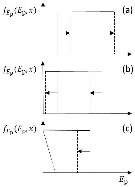
Figure 3 Schematic diagram of downslope changes in the distribution $f_{E_{\mathrm{p}}}(E_{\mathrm{p}},x)$ of particle energy states E_p (for simplicity a uniform distribution) due to the following: (a) gravitational advective heating in the absence of cooling; (b) advective frictional cooling in the absence of heating; and (c) net cooling. Arrows represent displacement occurring over a small downslope interval dx. The triangle represents an idealized situation in which, with net cooling, the likelihood of deposition increases with decreasing particle energy E_p and decreases with increasing energy. Note that an effect of deposition with heating or cooling is to increase the average energy 〈E_p〉 by culling lower-energy particles, thereby selecting higher-energy particles for continued travel with increasing distance.

We now offer a simple hypothesis describing the loss of energy associated with deposition. Recall that X_cA is a measure of the distance over which particles with energy E_p0 thermally collapse by frictional cooling. We may imagine, for example, a sudden removal of the source of heating such that X_cA is a measure of the distance of relaxation to a total loss of energy. For particles with energy E_p, this length scale can be expressed more generally as

$$\begin{array}{}\text{(44)}& l_{\mathrm{c}}\left(E_{\mathrm{p}}\right)\sim {\displaystyle \frac{\mathrm{4}{E}_{\mathrm{p}}\tan \mathit{\varphi }}{mg\stackrel{\mathrm{‾}}{{\mathit{\beta }}_x}\cos \mathit{\theta }}},\end{array}$$

which becomes unbounded only in the limit of $\mathit{\theta }\to \mathit{\pi }/\mathrm{2}$. Because thermal collapse involves deposition, we then assume at lowest order that

$$\begin{array}{}\text{(45)}& \mathit{\alpha }{l}_{\mathrm{c}}\left(E_{\mathrm{p}}\right){\displaystyle \frac{\partial n_{E_{\mathrm{p}}}\left(E_{\mathrm{p}},x\right)}{\partial x}}{|}_{\mathrm{d}}=-n_{E_{\mathrm{p}}}\left(E_{\mathrm{p}},x\right),\end{array}$$

where the subscript “d” denotes that the derivative refers to a change in the density $n_{E_{\mathrm{p}}}(E_{\mathrm{p}},x)$ just associated with deposition. We emphasize that Eq. (45) pertains to the imagined situation in which gravitational heating is not involved. This is the same as assuming a spatial Poisson process of deposition, that is, a fixed disentrainment rate keyed to the specific energy state E_p. In the presence of heating, however, the length scale of deposition increases relative to l_c. That is, heating suppresses the disentrainment rate. The factor α thus modulates the length scale l_c, so the product αl_c is a net e-folding length in the presence of heating. As described below, the factor α is assumed to be a function of the Kirkby number.

Substituting Eq. (45) into Eq. (17) and evaluating the integral then yields

$$\begin{array}{}\text{(46)}& \begin{array}{rl}\underset{\mathrm{0}}{\overset{\mathrm{\infty }}{\int }}& E_{\mathrm{p}}{\displaystyle \frac{\partial n_{E_{\mathrm{p}}}\left(E_{\mathrm{p}},x\right)}{\partial x}}{|}_{\mathrm{d}}\mathrm{d}{E}_{\mathrm{p}}\\ & =-{\displaystyle \frac{mg\cos \mathit{\theta }}{\mathit{\alpha }\mathrm{4}\tan \mathit{\varphi }}}\underset{\mathrm{0}}{\overset{\mathrm{\infty }}{\int }}\stackrel{\mathrm{‾}}{{\mathit{\beta }}_x}{n}_{E_{\mathrm{p}}}\left(E_{\mathrm{p}},x\right)\mathrm{d}{E}_{\mathrm{p}}\\ & =-{\displaystyle \frac{Nmg\langle {\mathit{\beta }}_x\rangle \cos \mathit{\theta }}{\mathit{\alpha }\mathrm{4}\tan \mathit{\varphi }}},\end{array}\end{array}$$

where we now redefine the Kirkby number as

$$\begin{array}{}\text{(47)}& \mathit{Ki}={\displaystyle \frac{\mathrm{4}\tan \mathit{\varphi }S}{\langle {\mathit{\beta }}_x\rangle }},\end{array}$$

assuming that $\stackrel{\mathrm{‾}}{{\mathit{\beta }}_x}$ is independent of E_p. Comparing this result with Eq. (33), the energy loss rate due to deposition is the same as the advective cooling rate but modulated by the factor α.

3.4 Conservation of mass revisited

The preceding material provides the basis for the next step, namely, calculating the disentrainment rate wherein effects of particle deposition on the energy balance are taken into account. Because $n_{E_{\mathrm{p}}}(E_{\mathrm{p}},x)\mathrm{d}{E}_{\mathrm{p}}$ represents the number of particles within the small energy interval E_p to E_p+dE_p, using Eqs. (44) and (45) the total disentrainment rate is therefore

$$\begin{array}{}\text{(48)}& \begin{array}{rl}{\displaystyle \frac{\mathrm{d}N\left(x\right)}{\mathrm{d}x}}& =\underset{\mathrm{0}}{\overset{\mathrm{\infty }}{\int }}{\displaystyle \frac{\partial n_{E_{\mathrm{p}}}\left(E_{\mathrm{p}},x\right)}{\partial x}}\mathrm{d}{E}_{\mathrm{p}}\\ & =-{\displaystyle \frac{mg\langle {\mathit{\beta }}_x\rangle \cos \mathit{\theta }}{\mathit{\alpha }\mathrm{4}\tan \mathit{\varphi }}}\underset{\mathrm{0}}{\overset{\mathrm{\infty }}{\int }}{\displaystyle \frac{\mathrm{1}}{E_{\mathrm{p}}}}{n}_{E_{\mathrm{p}}}\left(E_{\mathrm{p}},x\right)\mathrm{d}{E}_{\mathrm{p}}\\ & =-{\displaystyle \frac{Nmg\langle {\mathit{\beta }}_x\rangle \cos \mathit{\theta }}{\mathit{\alpha }\mathrm{4}\tan \mathit{\varphi }}}〈{\displaystyle \frac{\mathrm{1}}{E_{\mathrm{p}}}}〉.\end{array}\end{array}$$

Thus, the disentrainment rate is proportional to the cooling rate, as it should be. Here it is important to note that the expected value $\langle \mathrm{1}/E_{\mathrm{p}}\rangle \ne \mathrm{1}/\langle E_{\mathrm{p}}\rangle$. In fact, $\langle \mathrm{1}/E_{\mathrm{p}}\rangle$ is the reciprocal of the harmonic mean (Appendix F). This means that $\langle E_{\mathrm{p}}\rangle \langle \mathrm{1}/E_{\mathrm{p}}\rangle \ge \mathrm{1}$. Only in the limit where $n_{E_{\mathrm{p}}}(E_{\mathrm{p}},x)$ has zero variance does $\langle \mathrm{1}/E_{\mathrm{p}}\rangle \to \mathrm{1}/\langle E_{\mathrm{p}}\rangle$. To simplify the notation, hereafter we denote the arithmetic mean as 〈E_p〉=E_a and the harmonic mean as $\mathrm{1}/\langle \mathrm{1}/E_{\mathrm{p}}\rangle =E_{\mathrm{h}}$. Thus $E_{\mathrm{a}}/E_{\mathrm{h}}\ge \mathrm{1}$.

As a point of reference we may now define an ensemble-averaged deposition length as

$$\begin{array}{}\text{(49)}& L_{\mathrm{c}}\sim {\displaystyle \frac{\mathit{\alpha }\mathrm{4}\tan \mathit{\varphi }{E}_{\mathrm{h}}}{mg\langle {\mathit{\beta }}_x\rangle \cos \mathit{\theta }}}={\displaystyle \frac{\mathit{\alpha }{E}_{\mathrm{h}}}{mg\mathit{\mu }\cos \mathit{\theta }}},\end{array}$$

with $\mathit{\mu }=\langle {\mathit{\beta }}_x\rangle /\mathrm{4}\tan \mathit{\varphi }$. Note that in contrast to the energy-specific length scale l_c in Eqs. (44) and (45), L_c in Eq. (49) is keyed to the harmonic average energy of the ensemble. Setting θ=0 so that cos θ=1, the length scale L_c is entirely analogous to the length scale λ₀ used by Furbish and Haff (2010), Furbish and Roering (2013), and Doane et al. (2018) as the characteristic particle travel distance on a flat surface, thence modulated with increasing slope S (see also Sect. 5.3).

The factor α has a key role in the formulation. As described above, this factor modulates the length scale L_c in the presence of gravitational heating. Note that Eq. (48) is equivalent to

$$\begin{array}{}\text{(50)}& L_{\mathrm{c}}{\displaystyle \frac{\mathrm{d}N}{\mathrm{d}x}}=-N.\end{array}$$

For a given value of α the length scale L_c is set by the cooling rate, and this length scale increases with increasing slope angle θ. But gravitational heating also increases with θ, the effect of which is to suppress the rate of deposition and increase L_c. That is, the deposition length scale is not the same as the cooling length scale. As described below, whereas l_c is a measure of the rate of extraction of translational energy, this includes its conversion to rotational energy whose effect is to decrease the likelihood of stopping. On dimensional grounds an inspired guess suggests that this effect is a function f(Ki) of the Kirkby number Ki. For example, suppose that

$$\begin{array}{}\text{(51)}& L_{\mathrm{c}}={\displaystyle \frac{\mathit{\alpha }{E}_{\mathrm{h}}}{mg\mathit{\mu }\cos \mathit{\theta }}}={\displaystyle \frac{{\mathit{\alpha }}_{\mathrm{0}}{E}_{\mathrm{h}}}{mg\mathit{\mu }\cos \mathit{\theta }-mg{\mathit{\mu }}_{\mathrm{1}}\sin \mathit{\theta }}},\end{array}$$

where μ₁ is a coefficient of order unity. This leads to

$$\begin{array}{}\text{(52)}& \mathit{\alpha }={\displaystyle \frac{{\mathit{\alpha }}_{\mathrm{0}}}{\mathrm{1}-{\mathit{\mu }}_{\mathrm{1}}\mathit{Ki}}},\end{array}$$

where α→α₀ as μ₁Ki→0. Now,

$$\begin{array}{}\text{(53)}& L_{\mathrm{c}}={\displaystyle \frac{{\mathit{\alpha }}_{\mathrm{0}}{E}_{\mathrm{h}}}{mg\mathit{\mu }\cos \mathit{\theta }\left(\mathrm{1}-{\mathit{\mu }}_{\mathrm{1}}\mathit{Ki}\right)}}.\end{array}$$

This example suggests that L_c→∞ as μ₁Ki→1. That is, μ₁Ki→1 sets an upper limit above which deposition is insignificant. More generally we may write

$$\begin{array}{}\text{(54)}& L_{\mathrm{c}}={\displaystyle \frac{{\mathit{\alpha }}_{\mathrm{0}}f\left(\mathit{Ki}\right)E_{\mathrm{h}}}{mg\mathit{\mu }\cos \mathit{\theta }}},\end{array}$$

to indicate the possibility of other dependencies of α on Ki. Note that we provide evidence for this behavior in the companion paper, including the form of Eq. (52) based on experiments. For notational simplicity in subsequent sections, we use α with the understanding that this implies α=α₀f(Ki).

Here is a key sidebar for reference in our descriptions below of related formulations. We emphasize that according to Eqs. (45) and (48) the deposition rate is proportional to the advective cooling rate rather than the net cooling rate (the difference between the rates of heating and cooling), where the rate of heating then modulates the deposition rate, therein increasing the deposition length scale. Moreover, the deposition rate explicitly depends on the energy state of the particles. Consider a thought experiment. Let us imagine a system consisting of a box containing a finite number of particles. Suppose that we mechanically add energy to the system such that some proportion of the particles becomes a rarefied granular gas, and suppose that the gas achieves a non-equilibrium steady state with a specific average energy state (Appendix G). This means that the rate of (mechanical) heating is equal to the rate of cooling due to dissipative particle–box collisions, and sublimation (entrainment) matches deposition (disentrainment). That is, depending on the energy state of the particles, deposition occurs even though the difference between the rate of heating and cooling is zero. Now imagine that when a particle is deposited in our idealized box, it cannot become re-entrained (which is analogous to the hillslope system). The rate of heating and cooling of the remaining gas particles is still the same, yet the deposition process continues for those particles which, by chance, cool to sufficiently low energies for deposition to occur. Thus, we are assuming that the deposition rate is proportional to the cooling rate rather than the net cooling rate, depending on the energy state of the particles. The effect of heating is to decrease the likelihood of deposition by decreasing the proportion of particles that cool to sufficiently low energies for deposition to occur – which translates to suppressing the disentrainment rate and increasing the length scale of deposition. As outlined in Sect. 5 below, this effect is absent in previous formulations of particle disentrainment.

3.5 Energy and mass balances

We now collect results from above to summarize effects of the energy and mass balances. With $\mathit{\mu }=\langle {\mathit{\beta }}_x\rangle /\mathrm{4}\tan \mathit{\varphi }$ the total energy balance is given by

$$\begin{array}{}\text{(55)}& \begin{array}{rl}{\displaystyle \frac{\mathrm{d}E\left(x\right)}{\mathrm{d}x}}& =Nmg\sin \mathit{\theta }\\ & -Nmg\mathit{\mu }\cos \mathit{\theta }-{\displaystyle \frac{\mathrm{1}}{\mathit{\alpha }}}Nmg\mathit{\mu }\cos \mathit{\theta }.\end{array}\end{array}$$

To summarize, the first term on the right side of Eq. (55) is due to gravitational heating, the second term is due to frictional cooling, and the last term represents a loss of energy due to deposition. Note that none of these terms explicitly involves the energy E(x). In turn, conservation of mass is given by

$$\begin{array}{}\text{(56)}& {\displaystyle \frac{\mathrm{d}N\left(x\right)}{\mathrm{d}x}}=-{\displaystyle \frac{\mathrm{1}}{\mathit{\alpha }}}Nmg\mathit{\mu }\cos \mathit{\theta }{\displaystyle \frac{\mathrm{1}}{E_{\mathrm{h}}}}.\end{array}$$

This is coupled with Eq. (55) via the relation between the total energy E(x), the average energy E_a and the harmonic average energy E_h (see below), as well as the explicit appearance of N in both of these equations.

At this point we emphasize that the quantity $\mathit{\mu }=\langle {\mathit{\beta }}_x\rangle /\mathrm{4}\tan \mathit{\varphi }$ is not to be interpreted as Coulomb-like dynamic friction coefficient. Indeed, the product mgμcos θ in Eqs. (55) and (56) looks like an ordinary Coulomb friction force (e.g., Kirkby and Statham, 1975; Gabet and Mendoza, 2012). Recall, however, that cos θ enters from the geometry of particle motions and does not represent the angle needed to specify the normal component of the weight mg. Similarly, tan ϕ is an expected reflection angle, not a friction angle. We elaborate these points below.

To close the circle in reference to our stating point, Eq. (12), we now combine Eqs. (12), (55) and (56) to give

$$\begin{array}{}\text{(57)}& \begin{array}{rl}{\displaystyle \frac{\mathrm{d}{E}_{\mathrm{a}}\left(x\right)}{\mathrm{d}x}}& =mg\sin \mathit{\theta }-mg\mathit{\mu }\cos \mathit{\theta }\\ & +{\displaystyle \frac{mg\mathit{\mu }\cos \mathit{\theta }}{\mathit{\alpha }}}\left({\displaystyle \frac{E_{\mathrm{a}}}{E_{\mathrm{h}}}}-\mathrm{1}\right).\end{array}\end{array}$$

This balance involving the average energy E_a rather than the total energy E reveals an important behavior associated with deposition, centered on the parenthetical part of the last term. Namely, it is straightforward to show (Appendix F) that $E_{\mathrm{a}}/E_{\mathrm{h}}-\mathrm{1}\ge \mathrm{0}$. The last term in Eq. (57) therefore represents an apparent heating associated with deposition. With reference to Fig. 3, a net advective cooling uniformly lowers all particle energy states, thus lowering the average energy E_a as well as the total energy E. As this cooling lowers all energy states, some particles enter the range where deposition occurs, and the deposition rate therefore is proportional to the net advective cooling rate. In the absence of a net advective cooling, particles with small energy nonetheless are preferentially disentrained, so the average energy state increases. When cooling and deposition are combined, the average energy decreases more slowly than it otherwise would in the absence of deposition. This effect increases with increasing variance in the distribution of energies (Appendix F), and it vanishes as the variance goes to zero. The balance described by Eq. (57) thus provides a formal description of what we intuitively know: deposition culls lower-energy particles, thereby selecting higher-energy particles for continued travel with increasing distance. We note that Brilliantov et al. (2018) demonstrate an analogous unexpected behavior of granular gases, namely, the heating of a granular gas associated with particle aggregation with continued loss of total energy. This occurs when the rate of loss of particles by aggregation exceeds the rate of loss of total energy, such that by definition the average particle energy increases.

The balance described by Eq. (57) also reveals an important constraint on particle energies. Namely, if we imagine the special situation of isothermal conditions ($\mathrm{d}{E}_{\mathrm{a}}/\mathrm{d}x=\mathrm{0}$), then frictional cooling given by the second term on the right side of Eq. (57) must balance two sources of heating, namely, the first and third terms on the right side. This requires that either the Kirkby number Ki<1 or, if Ki=1, then the distribution $f_{E_{\mathrm{p}}}(E_{\mathrm{p}},x)$ of energies E_p must have zero variance such that E_h=E_a. Because this latter condition is highly unlikely, an isothermal condition generally requires that Ki<1. Conversely, net heating must occur with Ki>1.

According to Eq. (55) or Eq. (57), for a given slope angle θ the spatial rate of net cooling (or net heating) of the ensemble is a fixed quantity in which this slope angle has a dual role. Namely, an increasing slope decreases the rate of frictional cooling by decreasing the expected occurrence of particle–surface collisions, and it simultaneously increases the rate of gravitational heating. With θ=0, heating vanishes and frictional cooling occurs at a maximum rate of μmg. In turn, as $\mathit{\theta }\to \mathit{\pi }/\mathrm{2}$, which represents a vertical cliff, frictional cooling vanishes and heating matches that of free-fall motion. This transition from small to large slopes nicely illustrates what virtually every undergraduate student learns intuitively from the sport of boulder rolling (or “trundling”; Forrester, 1931), and why this sport is so spectacular and satisfying in steep terrain. Moreover, recall that the Kirkby number $\mathit{Ki}=S/\mathit{\mu }$ is the ratio of gravitational heating to advective cooling. If these are balanced, Ki=1 and

$$\begin{array}{}\text{(58)}& S=\mathit{\mu }={\displaystyle \frac{\langle {\mathit{\beta }}_x\rangle }{\mathrm{4}\tan \mathit{\varphi }}}.\end{array}$$

Qualitatively, this is the slope at which an undergraduate student may expect that boulder rolling starts to become particularly interesting.

The formulation also nicely illustrates that if the heating and cooling rates are matched, this does not imply an absence of deposition, as the last terms in Eqs. (55) and (57) may be finite with Ki=1. Moreover, because this is a probabilistic phenomenon, some particles are likely to become disentrained even on steep, rough slopes where heating on average exceeds cooling. Experienced undergraduates indeed inform us that some boulders just do not make it all the way to the bottom of the hillslope despite their best efforts to select conditions satisfying Ki>1.

4 General behavior

4.1 Effects of energy and mass balances

We now show how the energy and mass balances together lead to the generalized Pareto distribution of particle travel distances. To do this we restate Eqs. (55)–(57) in dimensionless form, which clearly reveals the important role of the Kirkby number Ki. Let E_a0 denote the initial average particle energy at x=0 and let N₀ denote the initial number of particles at x=0. In turn we define a characteristic cooling distance $X=E_{\mathrm{a}\mathrm{0}}/mg\mathit{\mu }\cos \mathit{\theta }$ so that E_a0=mgμcos θX. We now define the following dimensionless quantities denoted by circumflexes:

$$\begin{array}{}\text{(59)}& \begin{array}{rl}& x=X\widehat{x},N=N_{\mathrm{0}}\widehat{N},E=N_{\mathrm{0}}{E}_{\mathrm{a}\mathrm{0}}\widehat{E},\\ & E_{\mathrm{a}}=E_{\mathrm{a}\mathrm{0}}{\widehat{E}}_{\mathrm{a}}\mathrm{and}{E}_{\mathrm{h}}=E_{\mathrm{a}\mathrm{0}}{\widehat{E}}_{\mathrm{h}}.\end{array}\end{array}$$

With these definitions we write Eqs. (55)–(57) as

$$\begin{array}{}\text{(60)}& {\displaystyle }& {\displaystyle \frac{\mathrm{d}\widehat{E}\left(\widehat{x}\right)}{\mathrm{d}\widehat{x}}}=\left[\mathit{Ki}-\left(\mathrm{1}+{\displaystyle \frac{\mathrm{1}}{\mathit{\alpha }}}\right)\right]\widehat{N},\text{(61)}& {\displaystyle }& {\displaystyle \frac{\mathrm{d}\widehat{N}\left(\widehat{x}\right)}{\mathrm{d}\widehat{x}}}=-{\displaystyle \frac{\widehat{N}}{\mathit{\alpha }{\widehat{E}}_{\mathrm{h}}}}\mathrm{and}\text{(62)}& {\displaystyle }& {\displaystyle \frac{\mathrm{d}{\widehat{E}}_{\mathrm{a}}\left(\widehat{x}\right)}{\mathrm{d}\widehat{x}}}=\mathit{Ki}-\mathrm{1}+{\displaystyle \frac{\mathrm{1}}{\mathit{\alpha }}}\left({\displaystyle \frac{{\widehat{E}}_{\mathrm{a}}}{{\widehat{E}}_{\mathrm{h}}}}-\mathrm{1}\right).\end{array}$$

Because the dimensionless disentrainment rate ${\widehat{P}}_{\widehat{x}}\left(\widehat{x}\right)=-(\mathrm{1}/\widehat{N})\mathrm{d}\widehat{N}/\mathrm{d}\widehat{x}$, notice that Eq. (61) provides the basis for determining the distribution of travel distances using Eq. (4). This requires specifying how ${\widehat{E}}_{\mathrm{h}}$ varies with $\widehat{x}$ for given values of α and Ki. At this point, however, we must confront the fact that we have four unknowns, $\widehat{N}$, $\widehat{E}$, ${\widehat{E}}_{\mathrm{a}}$ and ${\widehat{E}}_{\mathrm{h}}$, and three equations, one of which is nonlinear in the ratio ${\widehat{E}}_{\mathrm{a}}/{\widehat{E}}_{\mathrm{h}}$. Here we add a fourth equation by assuming that this ratio remains fixed, namely,

$$\begin{array}{}\text{(63)}& {\displaystyle \frac{{\widehat{E}}_{\mathrm{a}}}{{\widehat{E}}_{\mathrm{h}}}}=\mathit{\gamma }.\end{array}$$

We do not know the distribution $f_{{\widehat{E}}_{\mathrm{p}}}\left({\widehat{E}}_{\mathrm{p}}\right)$ required to determine γ (Appendix F). Nonetheless, Eq. (63) essentially assumes that the form of $f_{{\widehat{E}}_{\mathrm{p}}}\left({\widehat{E}}_{\mathrm{p}}\right)$ remains similar with distance $\widehat{x}$. This allows us to illustrate key elements of the formulation.

With the assumption of Eq. (63) we note that Eq. (61) becomes

$$\begin{array}{}\text{(64)}& {\displaystyle \frac{\mathrm{d}\widehat{N}\left(\widehat{x}\right)}{\mathrm{d}\widehat{x}}}=-{\displaystyle \frac{\mathit{\gamma }\widehat{N}}{\mathit{\alpha }{\widehat{E}}_{\mathrm{a}}}},\end{array}$$

and Eq. (62) becomes

$$\begin{array}{}\text{(65)}& {\displaystyle \frac{\mathrm{d}{\widehat{E}}_{\mathrm{a}}\left(\widehat{x}\right)}{\mathrm{d}\widehat{x}}}=\mathit{Ki}-\mathrm{1}+{\displaystyle \frac{\mathrm{1}}{\mathit{\alpha }}}(\mathit{\gamma }-\mathrm{1}).\end{array}$$

Focusing initially on Eq. (65), isothermal conditions exist if $\mathrm{d}{\widehat{E}}_{\mathrm{a}}/\mathrm{d}\widehat{x}=\mathrm{0}$. We then rearrange Eqs. (62) or (65) to define a transition value of the Kirkby number, namely,

$$\begin{array}{}\text{(66)}& {\mathit{Ki}}_{*}=\mathrm{1}-{\displaystyle \frac{\mathrm{1}}{\mathit{\alpha }}}\left({\displaystyle \frac{{\widehat{E}}_{\mathrm{a}}}{{\widehat{E}}_{\mathrm{h}}}}-\mathrm{1}\right)=\mathrm{1}-{\displaystyle \frac{\mathrm{1}}{\mathit{\alpha }}}(\mathit{\gamma }-\mathrm{1}).\end{array}$$

If $\mathit{Ki}<{\mathit{Ki}}_{*}$, then cooling occurs ($\mathrm{d}{\widehat{E}}_{\mathrm{a}}/\mathrm{d}\widehat{x}<\mathrm{0}$); if $\mathit{Ki}>{\mathit{Ki}}_{*}$, then heating occurs ($\mathrm{d}{\widehat{E}}_{\mathrm{a}}/\mathrm{d}\widehat{x}>\mathrm{0}$). Recall that ${\widehat{E}}_{\mathrm{a}}/{\widehat{E}}_{\mathrm{h}}=\mathit{\gamma }\ge \mathrm{1}$ (Appendix F) so that $\mathit{\gamma }-\mathrm{1}\ge \mathrm{0}$. If the variance of energy states E_p is zero, then ${\widehat{E}}_{\mathrm{a}}/{\widehat{E}}_{\mathrm{h}}=\mathit{\gamma }=\mathrm{1}$, giving ${\mathit{Ki}}_{*}=\mathrm{1}$. Thus, in this case cooling occurs with Ki<1 and heating occurs with Ki>1. The ratio ${\widehat{E}}_{\mathrm{a}}/{\widehat{E}}_{\mathrm{h}}=\mathit{\gamma }$ generally increases with the variance of E_p, thus decreasing Ki_*. That is, as this variance increases, the transition between cooling and heating occurs at a smaller value of the Kirkby number. This represents a stronger culling (deposition) of lower-energy particles. The largest possible transition value is ${\mathit{Ki}}_{*}=\mathrm{1}$.

We now start with an idealized example that illustrates key elements of the formulation, including the coupling between Eqs. (60)–(62). Assume that the Kirkby number Ki is fixed, and assume isothermal conditions. Thus $\mathrm{d}{\widehat{E}}_{\mathrm{a}}/\mathrm{d}\widehat{x}=\mathrm{0}$ with ${\widehat{E}}_{\mathrm{a}}={\widehat{E}}_{\mathrm{a}\mathrm{0}}$ so that Eq. (62) leads to

$$\begin{array}{}\text{(67)}& {\widehat{E}}_{\mathrm{h}}={\displaystyle \frac{{\widehat{E}}_{\mathrm{a}\mathrm{0}}}{\mathrm{1}+\mathit{\alpha }(\mathrm{1}-\mathit{Ki})}}.\end{array}$$

With ${\widehat{E}}_{\mathrm{a}}/{\widehat{E}}_{\mathrm{h}}={\widehat{E}}_{\mathrm{a}\mathrm{0}}/{\widehat{E}}_{\mathrm{h}}=\mathit{\gamma }$, then $\mathit{\gamma }=\mathrm{1}+\mathit{\alpha }(\mathrm{1}-\mathit{Ki})$. The disentrainment rate ${\widehat{P}}_{\widehat{x}}\left(\widehat{x}\right)=-(\mathrm{1}/\widehat{N})\mathrm{d}\widehat{N}/\mathrm{d}\widehat{x}$. Thus, according to Eqs. (61) and (67),

$$\begin{array}{}\text{(68)}& {\widehat{P}}_{\widehat{x}}\left(\widehat{x}\right)={\displaystyle \frac{\mathrm{1}+\mathit{\alpha }(\mathrm{1}-\mathit{Ki})}{\mathit{\alpha }{\widehat{E}}_{\mathrm{a}\mathrm{0}}}}={\displaystyle \frac{\mathit{\gamma }}{\mathit{\alpha }{\widehat{E}}_{\mathrm{a}\mathrm{0}}}}.\end{array}$$

In turn, using Eq. (4) this yields an exponential distribution of travel distances with mean

$$\begin{array}{}\text{(69)}& {\mathit{\mu }}_{\widehat{x}}={\displaystyle \frac{\mathit{\alpha }{\widehat{E}}_{\mathrm{a}\mathrm{0}}}{\mathrm{1}+\mathit{\alpha }(\mathrm{1}-\mathit{Ki})}}={\displaystyle \frac{\mathit{\alpha }{\widehat{E}}_{\mathrm{a}\mathrm{0}}}{\mathit{\gamma }}},\end{array}$$

so that

$$\begin{array}{}\text{(70)}& \widehat{N}\left(\widehat{x}\right)={\displaystyle \frac{\mathrm{1}}{{\mathit{\mu }}_{\widehat{x}}}}{e}^{-\widehat{x}/{\mathit{\mu }}_{\widehat{x}}}.\end{array}$$

Note that an increasing value of γ in Eq. (69) represents an increasing proportion of lower-energy particles available for deposition relative to this availability with γ→1, the effect of which is to decrease the mean travel distance.

The total energy $\widehat{E}$ also declines exponentially with $\widehat{x}$. Namely, substituting Eq. (70) into Eq. (60) leads to

$$\begin{array}{}\text{(71)}& \begin{array}{rl}\widehat{E}\left(\widehat{x}\right)& =\mathrm{1}-{\displaystyle \frac{\mathrm{1}}{\mathit{\alpha }}}[\mathrm{1}+\mathit{\alpha }(\mathrm{1}-\mathit{Ki}\left)\right]\left(\mathrm{1}-e^{-\widehat{x}/{\mathit{\mu }}_{\widehat{x}}}\right)\\ & =\mathrm{1}-{\displaystyle \frac{\mathit{\gamma }}{\mathit{\alpha }}}\left(\mathrm{1}-e^{-\widehat{x}/{\mathit{\mu }}_{\widehat{x}}}\right).\end{array}\end{array}$$

This example of isothermal conditions illustrates that with ${\widehat{E}}_{\mathrm{a}}={\widehat{E}}_{\mathrm{a}\mathrm{0}}$, then according to Eq. (69) the average travel distance ${\mathit{\mu }}_{\widehat{x}}$ is directly proportional to the initial average energy. However, isothermal conditions are unlikely, because according to Eq. (66), such a condition requires a specific value of Ki for the ratio ${\widehat{E}}_{\mathrm{a}}/{\widehat{E}}_{\mathrm{h}}=\mathit{\gamma }$. We now consider the more general case involving either net cooling or net heating.

As above we assume that the ratio ${\widehat{E}}_{\mathrm{a}}/{\widehat{E}}_{\mathrm{h}}=\mathit{\gamma }$ is fixed, although the averages ${\widehat{E}}_{\mathrm{a}}$ and ${\widehat{E}}_{\mathrm{h}}$ otherwise are unconstrained. Net cooling or net heating is not prescribed; either condition is allowed. Using Eqs. (60) and (61) the disentrainment rate is (Appendix H)

$$\begin{array}{}\text{(72)}& {\widehat{P}}_{\widehat{x}}\left(\widehat{x}\right)={\displaystyle \frac{\mathrm{1}}{a\widehat{x}+b}},\end{array}$$

where

$$\begin{array}{}\text{(73)}& \begin{array}{rl}& a={\displaystyle \frac{\mathit{\alpha }}{\mathit{\gamma }}}\left(\mathit{Ki}-\mathrm{1}+{\displaystyle \frac{\mathit{\gamma }}{\mathit{\alpha }}}-{\displaystyle \frac{\mathrm{1}}{\mathit{\alpha }}}\right)={\displaystyle \frac{\mathit{\alpha }}{\mathit{\gamma }}}\left(\mathit{Ki}-{\mathit{Ki}}_{*}\right)\mathrm{and}\\ & b={\displaystyle \frac{\mathit{\alpha }{\widehat{E}}_{\mathrm{a}\mathrm{0}}}{\mathit{\gamma }}}.\end{array}\end{array}$$

Note that as a→0 the disentrainment rate goes to a fixed value equal to $\mathrm{1}/b=\mathit{\gamma }/\mathit{\alpha }{\widehat{E}}_{\mathrm{a}\mathrm{0}}$, and the distribution $f_{\widehat{x}}\left(\widehat{x}\right)$ of travel distances $\widehat{x}$ goes to an exponential distribution with mean ${\mathit{\mu }}_{\widehat{x}}=b=\mathit{\alpha }{\widehat{E}}_{\mathrm{a}\mathrm{0}}/\mathit{\gamma }$. A value of a>0 ($\mathit{Ki}>{\mathit{Ki}}_{*}$) implies decreasing disentrainment with increasing x. A value of a<0 ($\mathit{Ki}<{\mathit{Ki}}_{*}$) implies increasing disentrainment.

More generally, the distribution of travel distances is a generalized Pareto distribution with position parameter equal to zero (Appendix H), namely,

$$\begin{array}{}\text{(74)}& f_{\widehat{x}}\left(\widehat{x}\right)={\displaystyle \frac{b^{\mathrm{1}/a}}{(a\widehat{x}+b{)}^{\mathrm{1}+\mathrm{1}/a}}},\end{array}$$

where now a∈ℝ is interpreted as a shape parameter and b>0 is a scale parameter (Pickands, 1975; Hosking and Wallis, 1987). The cumulative distribution is

$$\begin{array}{}\text{(75)}& {\widehat{F}}_{\widehat{x}}\left(\widehat{x}\right)=\left\{\begin{array}{ll}\mathrm{1}-\frac{b^{\mathrm{1}/a}}{(a\widehat{x}+b{)}^{\mathrm{1}/a}}& a\ne \mathrm{0}\\ \mathrm{1}-e^{-\widehat{x}/b}& a=\mathrm{0}\end{array}\right.,\end{array}$$

and the exceedance probability is

$$\begin{array}{}\text{(76)}& {\widehat{R}}_{\widehat{x}}\left(\widehat{x}\right)=\left\{\begin{array}{ll}\frac{b^{\mathrm{1}/a}}{(a\widehat{x}+b{)}^{\mathrm{1}/a}}& a\ne \mathrm{0}\\ e^{-\widehat{x}/b}& a=\mathrm{0}\end{array}\right..\end{array}$$

For a<1 the mean is

$$\begin{array}{}\text{(77)}& {\mathit{\mu }}_{\widehat{x}}={\displaystyle \frac{b}{\mathrm{1}-a}}={\displaystyle \frac{\mathit{\alpha }{\widehat{E}}_{\mathrm{a}\mathrm{0}}}{\mathrm{1}+\mathit{\alpha }-\mathit{\alpha }\mathit{Ki}}},\end{array}$$

which is independent of the ratio $\mathit{\gamma }={\widehat{E}}_{\mathrm{a}}/{\widehat{E}}_{\mathrm{h}}$. This is the same as Eq. (69) for isothermal conditions, although the denominator in Eq. (77) generally is not equal to γ. In turn, Eq. (77) requires that

$$\begin{array}{}\text{(78)}& \mathit{Ki}<\mathrm{1}+{\displaystyle \frac{\mathrm{1}}{\mathit{\alpha }}},\end{array}$$

which provides the upper limit of Ki for which the mean ${\mathit{\mu }}_{\widehat{x}}$ is defined. Because α>0, this limit may be greater than one. For $a<\mathrm{1}/\mathrm{2}$ the variance is

$$\begin{array}{}\text{(79)}& \begin{array}{rl}{\mathit{\sigma }}_{\widehat{x}}^{\mathrm{2}}& ={\displaystyle \frac{b^{\mathrm{2}}}{(\mathrm{1}-a{)}^{\mathrm{2}}(\mathrm{1}-\mathrm{2}a)}}\\ & ={\displaystyle \frac{{\mathit{\alpha }}^{\mathrm{2}}{\widehat{E}}_{\mathrm{a}\mathrm{0}}^{\mathrm{2}}}{(\mathrm{1}+\mathit{\alpha }-\mathit{\alpha }\mathit{Ki}{)}^{\mathrm{2}}(\mathrm{2}/\mathit{\gamma }+\mathrm{2}\mathit{\alpha }/\mathit{\gamma }-\mathrm{1}-\mathrm{2}\mathit{\alpha }\mathit{Ki}/\mathit{\gamma })}}.\end{array}\end{array}$$

Unlike the mean, the variance depends on $\mathit{\gamma }={\widehat{E}}_{\mathrm{a}}/{\widehat{E}}_{\mathrm{h}}$. In turn, for a≥1 such that

$$\begin{array}{}\text{(80)}& \mathit{Ki}\ge \mathrm{1}+{\displaystyle \frac{\mathrm{1}}{\mathit{\alpha }}},\end{array}$$

the mean of $f_{\widehat{x}}\left(\widehat{x}\right)$ is undefined. Moreover, for $a\ge \mathrm{1}/\mathrm{2}$ the variance is undefined. These results reflect the heavy-tailed behavior of the generalized Pareto distribution.

As a point of reference in the second companion paper (Furbish et al., 2021a), the generalized Pareto distribution defined by Eq. (74) also may be considered a generalized Lomax distribution. This distribution can be rewritten as an ordinary Lomax distribution (Appendix H). Namely, if we define the shape parameter $a_{\mathrm{L}}=\mathrm{1}/a$ and the scale parameter $b_{\mathrm{L}}=b/a$, then Eq. (74) becomes

$$\begin{array}{}\text{(81)}& f_{\widehat{x}}\left(\widehat{x}\right)={\displaystyle \frac{a_{\mathrm{L}}{b}_{\mathrm{L}}^{a_{\mathrm{L}}}}{{\left(\widehat{x}+b_{\mathrm{L}}\right)}^{\mathrm{1}+a_{\mathrm{L}}}}}{a}_{\mathrm{L}},b_{\mathrm{L}}>\mathrm{0},\end{array}$$

which is a Lomax distribution with mean

$$\begin{array}{}\text{(82)}& {\mathit{\mu }}_{\widehat{x}}={\displaystyle \frac{b_{\mathrm{L}}}{a_{\mathrm{L}}-\mathrm{1}}}{a}_{\mathrm{L}}>\mathrm{1}.\end{array}$$

For a_L>0 (a>0) the forms and behaviors of Eqs. (74) and (81) are identical. Notice, however, that if a<0 then $a_{\mathrm{L}}=\mathrm{1}/a<\mathrm{0}$ and $b_{\mathrm{L}}=b/a<\mathrm{0}$ for positive b. This means that we cannot use the form of the Lomax distribution given by Eq. (81) to examine conditions involving a<0. Yet these conditions are mechanically meaningful, so we proceed using the generalized Pareto distribution given by Eq. (74). To be clear, the ordinary Pareto distribution that is normally referred to in the literature is a special case of the generalized Pareto distribution. In turn the Lomax distribution is a special case of the Pareto distribution (and therefore of the generalized Pareto) with position parameter equal to zero.

With reference to Fig. 4, for a<0 the distribution $f_{\widehat{x}}\left(\widehat{x}\right)$ is bounded at a value of $\widehat{x}=b/\left|a\right|$ with a mean given by Eq. (77). This represents a condition of rapid thermal collapse. Specifically, when $a<-\mathrm{1}$ this distribution monotonically increases and becomes asymptotically unbounded at $\widehat{x}=b/\left|a\right|$. In the limit of $a\to -\mathrm{1}$ it becomes a uniform distribution. When $a=-\mathrm{1}/\mathrm{2}$ this distribution is triangular. For $-\mathrm{1}/\mathrm{2}<a<\mathrm{0}$ this distribution decays more rapidly than an exponential distribution and is bounded at the position $\widehat{x}=b/\left|a\right|$. For a=0, $f_{\widehat{x}}\left(\widehat{x}\right)$ becomes an exponential distribution, representing an isothermal condition as described above. For a>0 the distribution $f_{\widehat{x}}\left(\widehat{x}\right)$ is heavy-tailed. This represents a condition of net heating. Specifically, for $\mathrm{0}<a<\mathrm{1}/\mathrm{2}$ this distribution decays more slowly than an exponential distribution, but it possesses a finite mean and a finite variance. For $\mathrm{1}/\mathrm{2}\le a<\mathrm{1}$ the distribution possesses a finite mean, but its variance is undefined. For a≥1 the mean and variance of $f_{\widehat{x}}\left(\widehat{x}\right)$ are both undefined, even though this distribution properly integrates to unity. For a>0 the tail of $f_{\widehat{x}}\left(\widehat{x}\right)$ decays as a power function, namely, $f_{\widehat{x}}\left(\widehat{x}\right)\sim {\widehat{x}}^{-(\mathrm{1}+\mathrm{1}/a)}$. The exceedance probability decays as $R_{\widehat{x}}\left(\widehat{x}\right)\sim {\widehat{x}}^{-\mathrm{1}/a}$. These results are summarized in Table 1. We provide evidence of all three behaviors – rapid thermal collapse, isothermal conditions, and net heating – in our second companion paper (Furbish et al., 2021a).

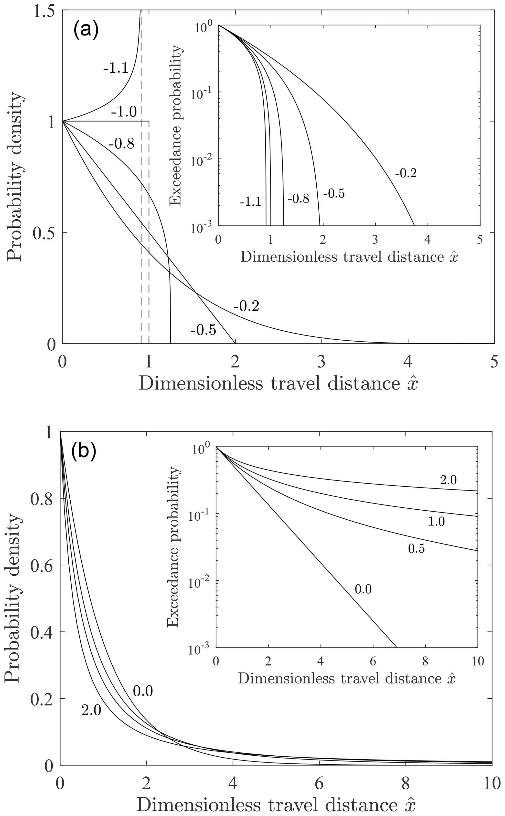
Figure 4 Plot of probability density $f_{\widehat{x}}\left(\widehat{x}\right)$ versus travel distance $\widehat{x}$ for scale parameter b=1 and different values of the shape parameter a for (a) a<0 and (b) a≥0 with associated exceedance probability plots (insets). Compare with Fig. 1 in Hosking and Wallis (1987).

Table 1 Behavior of the generalized Pareto distribution associated with the shape parameter a and Kirkby number Ki as illustrated in Fig. 4.

¹ Truncation occurs at dimensionless distance $\widehat{x}=b/\left|a\right|$. ² Triangular with $a=-\mathrm{1}/\mathrm{2}$.

The formulation above assumes uniform surface conditions, specifically, uniform slope angle and roughness texture. We show below (Sect. 6) how it may be adapted to varying downslope conditions. We also note that the distribution $f_{\widehat{x}}\left(\widehat{x}\right)$ given by Eq. (74) can be incorporated into a mixed distribution. Indeed, a mixed distribution is the natural choice for describing the travel distances of a mixture of particle sizes, each involving a different frictional cooling behavior for a given surface roughness (Roth et al., 2020).

4.2 Elements of the average travel distance

The average travel distance given by Eq. (77) for $\mathit{Ki}<\mathrm{1}+\mathrm{1}/\mathit{\alpha }$ contains all of the elements that influence particle motions except the quantity γ. Thus, whereas the average by itself does not reveal the source of variations in the form of distribution of travel distances, Eq. (74), the average nonetheless provides a focal point. Here we rewrite this average in its dimensional form, then step through the significance of its elements. Namely, with $E_{\mathrm{a}\mathrm{0}}=(\mathrm{1}/\mathrm{2})m\langle u_{\mathrm{0}}^{\mathrm{2}}\rangle$ and $\mathit{Ki}=S/\mathit{\mu }=(\mathrm{1}/\mathit{\mu })mg\sin \mathit{\theta }/mg\cos \mathit{\theta }$,

$$\begin{array}{}\text{(83)}& \begin{array}{rl}{\mathit{\mu }}_x& ={\displaystyle \frac{E_{\mathrm{a}\mathrm{0}}}{mg\mathit{\mu }\cos \mathit{\theta }}}{\displaystyle \frac{\mathit{\alpha }}{\mathrm{1}+\mathit{\alpha }-\mathit{\alpha }\mathit{Ki}}}\\ & ={\displaystyle \frac{E_{\mathrm{a}\mathrm{0}}}{(\mathrm{1}+\mathrm{1}/\mathit{\alpha })mg\mathit{\mu }\cos \mathit{\theta }-mg\sin \mathit{\theta }}}.\end{array}\end{array}$$

For an ensemble of particles whose motions start at x=0, the average travel distance μ_x increases directly with the average starting energy $E_{\mathrm{a}\mathrm{0}}\propto \langle u_{\mathrm{0}}^{\mathrm{2}}\rangle$. This is entirely akin to the formulation by Kirkby and Statham (1975) (see below), and it highlights the significance of the initial particle energy conditions at x=0 in setting their travel distances. The archetypal example involves rockfall from cliffs followed by their motions over talus and scree slope surfaces (Fig. 1), where fall heights and initial rebounds set the initial average downslope energy. This also is a key element in experiments where initial energies are set by the choice of drop height (Kirkby ana Statham, 1975) or launch speed (Gabet and Mendoza, 2012; DiBiase et al., 2017). This aspect of the formulation also points to the significance of energetics associated with the entrainment rate E_s(x) in Eqs. (5) and (6) at hillslope positions that are not necessarily as well-defined as, say, the base of a cliff (see Sect. 6).

The average travel distance μ_x is inversely proportional to the rate of frictional cooling represented by mgμcos θ. Here we reemphasize that despite its form, this expression does not represent a Coulomb-like friction. Rather, this expression enters the formulation via the characteristic length λ in setting the expected number of collisions per unit distance, n_x. As described below, the surface-normal component of the particle weight does not set collisional friction; this is set by dynamic forces during collisions. Moreover, the appearance of the Kirkby number Ki in the denominator of Eq. (83) indicates that as Ki increases, the denominator becomes smaller (subject to the conditions that $\mathit{Ki}<\mathrm{1}+\mathrm{1}/\mathit{\alpha }$), so the average travel distance increases. We also note that, except for purely bouncing motions, it is incorrect to interpret the length λ strictly as a saltation-like distance. This is a scaling approximation (Appendix D) to show that n_x must involve the average energy (∝〈u²〉) and the geometrical factor cos θ at lowest order.

Notice that Eq. (83) indicates that with $E_{\mathrm{a}\mathrm{0}}=(\mathrm{1}/\mathrm{2})m\langle u_{\mathrm{0}}^{\mathrm{2}}\rangle$ the average travel distance μ_x is independent of the particle mass m. Viewed in isolation, this suggests that large particles should on average travel no farther than small particles. However, this is inconsistent with what is observed in laboratory and field-based experiments (Kirkby and Statham, 1975; DiBiase et al., 2017; Roth et al., 2020) and with downslope size sorting on natural talus and scree slopes (Statham, 1976). We examine this topic in the second companion paper (Furbish et al., 2021a); here we offer a synopsis, which centers on the interpretation and significance of the quantities μ and α.

Recall that the formulation is based on the assumption that a change in translational kinetic energy ΔE_p associated with a particle–surface collision can be expressed as $\mathrm{\Delta }{E}_{\mathrm{p}}=-{\mathit{\beta }}_x{E}_{\mathrm{p}}$ so that ${\mathit{\beta }}_x=-\mathrm{\Delta }{E}_{\mathrm{p}}/E_{\mathrm{p}}$ is the proportion of the energy extracted during the collision. Both ΔE_p and β_x are random variables. As described in Appendix E, in general we may write the energy balance of a particle as

$$\begin{array}{}\text{(84)}& \mathrm{\Delta }{E}_{\mathrm{p}}=-\mathrm{\Delta }{E}_{\mathrm{r}}-f_{\mathrm{c}}-f_y.\end{array}$$

Here, a positive change in rotational energy ΔE_r is seen as an extraction of translational energy. This loss of translational energy with the onset of rotation may be relatively large if a collision involves stick following initial sliding due to a large normal impulse, and such a loss also may occur due to the imposed torque of friction during a collision that does not necessarily involve stick. The term f_c in Eq. (84) represents losses associated with particle and surface deformation as well as work performed against friction during collision impulses (thence converted to heat, sound, etc.). But this term also includes losses associated with deformation of the surface at a scale larger than that of an idealized particle–surface impulse contact, namely, due to momentum exchanges associated with the sputtering of loose surface particles during collision. (The videos published as supplementary material to DiBiase et al. (2017) nicely illustrate this sputtering as well as the onset of rotational motion.) The term f_y in Eq. (84) represents the energy loss associated with glancing collisions that produce transverse translational motions and rotation oriented differently than any incident rotation. In some cases the change in energy ΔE_p can be expressed directly in terms of the energy state E_p (Appendix E). However, the complexity of particle–surface collisions on natural hillslopes precludes explicitly demonstrating such a relation for all possible scenarios. Nonetheless, it is entirely defensible to assume that energy losses can be related to the energy state E_p if the elements involved are formally viewed as random variables. Then, the simple relation $\mathrm{\Delta }{E}_{\mathrm{p}}=-{\mathit{\beta }}_x{E}_{\mathrm{p}}$ is to be viewed as a hypothesis to be tested against data.

This hypothesis formally enters the formulation via the right side of Eq. (58). Namely, from this relation we may write μ∼〈β_x〉, highlighting that μ is associated with the cooling rate. In turn, particle collision mechanics (Appendix E) suggest, for example, that $\mathit{\mu }\sim \langle {\mathit{\beta }}_x\rangle \sim M\left(\mathit{\theta }\right)$, where M(θ) involves the coefficients associated with tangential and normal impulses contributing to energy losses during collisions and depends on the slope angle θ in that the expected surface normal impact velocity varies with this angle. (In an idealized particle–surface collision these coefficients include the normal coefficient of restitution and a coefficient describing the ratio of tangential to normal impulses during the collision (e.g., Brach, 1991; Brach and Dunn, 1992, 1995).) Moreover, M(θ) is independent of particle size.

In turn, focusing on the definition of the deposition length scale L_c, Eq. (51), α may be viewed as representing a direct effect of heating described by mgsin θ, namely, to decrease the likelihood of deposition by decreasing the proportion of particles that cool to sufficiently low energies for deposition to occur – which translates to suppressing the disentrainment rate and increasing the length scale of deposition L_c relative to the cooling length scale $l_{\mathrm{c}}=E_{\mathrm{h}}/mg\mathit{\mu }\cos \mathit{\theta }$. Specifically, heating decreases the spatial rate of the Poisson deposition process below that which would occur in the absence of heating. In this view, μ goes with the cooling rate (not the deposition rate). But we also may write Eq. (51) as in Eq. (53). Viewed in this manner, we may define an apparent friction factor as ${\mathit{\mu }}_{\mathrm{0}}=\mathit{\mu }(\mathrm{1}-{\mathit{\mu }}_{\mathrm{1}}\mathit{Ki})$ associated with deposition. Here again, μ is associated with the cooling rate but is then modulated by heating. We suggest in the second companion paper (Furbish et al. 2021a) that for the same particle size, α increases with increasing Ki, very likely due to a combination of increased heating and increased partitioning of translational energy to rotational motion (Dorren, 2003; Luckman, 2013) – both decreasing the likelihood of stopping and not represented in just the factor μ. We also suggest that for the same slope and surface roughness, α increases with increasing particle size, decreasing the likelihood of frictional loss with increasing rotation.

Turning to the factor γ (which does not appear in Eq. 83), recall that an increasing value (γ>1) reflects an increasing availability of low-energy particles for deposition. Here is what we know. On the one hand, γ cannot be close to unity with randomization of motions by collisional friction, or if the initial downslope energies E_p0 are not a fixed value. That is, if the distribution of energies $f_{E_{\mathrm{p}}}(E_{\mathrm{p}},\mathrm{0})$ has finite variance, then γ>1. On the other hand, γ cannot be very large, or deposition would dominate over small distances without long motions that are observed – unless the Kirkby number Ki is unrealistically large. It is possible to qualitatively explore possible values of γ based on assuming different forms of the distribution of energies (and we have done this), but in the absence of knowing the specific form of the distribution, this exercise is not particularly meaningful. In the companion paper we show that fits of experimental travel distances to the theoretical distribution f_x(x) are relatively insensitive to the specific value of γ selected.

5 Related formulations

Here we briefly examine three related formulations of particle disentrainment, focusing on the mechanical basis of this work for comparison with the formulation above. (We examine associated experiments in the companion paper.) We start with the formulations of Kirkby and Statham (1975) and Gabet and Mendoza (2012). These begin with descriptions of particle motions over time rather than space, centered on consideration of a combination of momentum and energy. We then consider elements of the probabilistic formulation presented by Furbish and Haff (2010), Furbish and Roering (2013), and Doane et al. (2018).

5.1 Kirkby–Statham formulation

In their study of particle motions on scree surfaces, Kirkby and Statham (1975) start with a statement of conservation of energy for a particle falling from height h at x=0 onto a rough surface inclined at an angle θ. Namely, if $w_{\mathrm{0}}=\sqrt{\mathrm{2}gh}$ is the vertical impact velocity, then it is assumed that the initial downslope velocity on average is u₀=w₀sin θ. (This actually should be u₀=ϵw₀sin θ with the normal coefficient of restitution ϵ.) The initial downslope particle energy therefore is $(\mathrm{1}/\mathrm{2})m{u}_{\mathrm{0}}^{\mathrm{2}}={\mathit{ϵ}}^{\mathrm{2}}mgh{\sin }^{\mathrm{2}}\mathit{\theta }=E_{\mathrm{p}\mathrm{0}}$. In turn, because work is W=F_xl, where F_x is the downslope force and l is a displacement, then for a fixed force F_x the displacement is $l=W/F_x$. Assuming that W must be equal to the initial kinetic energy E_p0 (that is, this initial energy is dissipated over the distance l), then $l=E_{\mathrm{p}\mathrm{0}}/F_x$. Assuming a Coulomb-like friction behavior, $F_x=mg\sin \mathit{\theta }-{\mathit{\mu }}_{\mathrm{d}}mg\cos \mathit{\theta }$, where μ_d is a dynamic friction coefficient. Upon asserting that the length l represents the expected travel distance μ_x,

$$\begin{array}{}\text{(85)}& {\mathit{\mu }}_x=-{\displaystyle \frac{E_{\mathrm{p}\mathrm{0}}}{mg\sin \mathit{\theta }-{\mathit{\mu }}_{\mathrm{d}}mg\cos \mathit{\theta }}}=-{\displaystyle \frac{{\mathit{ϵ}}^{\mathrm{2}}h{\sin }^{\mathrm{2}}\mathit{\theta }}{\sin \mathit{\theta }-{\mathit{\mu }}_{\mathrm{d}}\cos \mathit{\theta }}},\end{array}$$

where it is assumed that $\left|{\mathit{\mu }}_{\mathrm{d}}\cos \mathit{\theta }\right|\ge \sin \mathit{\theta }$. As described below, this is equivalent to assuming that particle energy decreases linearly with distance.

This formulation correctly describes the motion of an individual particle that experiences a fixed Coulomb-like friction force, but it cannot represent the rarefied behavior of an ensemble of particles. Nonetheless, it shares elements of the preceding formulation. Namely, in comparing Eq. (85) with Eq. (83), let us momentarily set aside the fact that E_p0 cannot represent E_a0 except in the limit of zero variance of initial energy states (γ=1) and that the friction factor μ in Eq. (83) and the dynamic friction coefficient μ_d in Eq. (85) have different interpretations. These two descriptions of the average travel distance μ_x then converge in the limit of α→∞. Inasmuch as Eq. (52) correctly describes the behavior of α, this limit coincides with Ki→1.

More generally, Eq. (85) implies that the deposition rate is independent of the extant energy state of particles. If Eq. (85) denotes the average of a distribution of travel distances with fixed disentrainment rate, then this fixed rate $P_x=\mathrm{1}/{\mathit{\mu }}_x$. In dimensionless form this is

$$\begin{array}{}\text{(86)}& P_{\widehat{x}}={\displaystyle \frac{\mathrm{1}-\mathit{Ki}}{{\widehat{E}}_{\mathrm{p}\mathrm{0}}}}.\end{array}$$

That is, Eq. (86) cannot allow for the possibility of variations in the cooling rate or heating rate that give spatial variations in the disentrainment rate, as in Eq. (72). The resulting distribution f_x(x) of travel distances therefore is exponential for all Ki<1.

Interestingly, the formulation of Kirkby and Statham (1975) is equivalent to (Appendix I)

$$\begin{array}{}\text{(87)}& {\displaystyle \frac{\mathrm{d}{E}_{\mathrm{p}}}{\mathrm{d}x}}=mg\sin \mathit{\theta }-mg{\mathit{\mu }}_{\mathrm{d}}\cos \mathit{\theta }.\end{array}$$

This is like Eq. (57) but lacks the heating effect of deposition. Like Eq. (85), Eq. (87) implies that deposition is independent of the extant energy state; when Ki=1 the energy E_p remains fixed as x→∞ (again noting that E_p0 cannot represent E_a0 except in the limit of zero variance of initial energy states).

Dorren (2003) provides a review of efforts to elaborate the Kirkby–Statham description of particle motions in relation to hazard assessment. These mostly appeal to a Coulomb-like frictional behavior and are focused on predicting rockfall runout distances.

5.2 Gabet–Mendoza formulation

In support of their experimental work involving particle motions on a rough, inclined surface, Gabet and Mendoza (2012) appeal to ideas from Quartier et al. (2000) and Samson et al. (1998) and assume that particle acceleration is described as a linear combination of the gravitational force, a Coulomb-like friction and collisional friction, namely,

$$\begin{array}{}\text{(88)}& {\displaystyle \frac{\mathrm{d}u\left(t\right)}{\mathrm{d}t}}=g\sin \mathit{\theta }-{\mathit{\mu }}_{\mathrm{d}}g\cos \mathit{\theta }-\mathit{\kappa }{u}^{\mathit{\psi }}.\end{array}$$

As written, the dimensions of the coefficient κ depend on the value of the exponent ψ, which is thought to vary between one and two based on experiments. The principal significance of this formulation is that it points to the role of collisional friction – which Quartier et al. (2000) demonstrate is the principle source of energy dissipation in their experiments – and thus represents an important step beyond the Coulomb-like model of Kirkby and Statham (1975). However, because there is confusion in the literature regarding the form and interpretation of Eq. (88), we summarize the basis of this formulation in Appendix J. The essence is this: the Coulomb term and the collisional term as written are not additive for an individual particle. The collisional term is a stochastic quantity and applies to an averaged behavior, not to the instantaneous behavior of an individual particle. If this term is involved, the velocity u must be considered a time-averaged or ensemble-averaged velocity, or Eq. (88) must be recast as a Langevin-like equation. Parts of this formulation are appropriate for describing the behavior of particles that roll bumpety-bump over a surface roughened with a monolayer of particles, but for the reasons described above and in Appendix J the deterministic, continuous form of this formulation is not well matched to the mechanics involved in rarefied motions over the roughness of natural hillslopes.

In both formulations above the idea of a Coulomb-like friction with a dynamic friction coefficient is mechanically unsound (Appendix J). For particles that tumble, bounce and skitter down a rough surface, the static normal weight of a particle, mgcos θ, does not set the particle–surface friction. Rather, dynamic forces during collision impulses matter (Brach, 1991; Stronge, 2000). This includes the dynamic Coulomb-like friction force associated with conversion of translational to rotational kinetic energy during collisions (Appendix E). Formulating a dynamic friction coefficient would require ensemble averaging of the ratio of tangential to normal momentum exchanges, both of which are random variables. A Coulomb-like friction is appropriate for solid body and dense granular motions, but not for the rarefied conditions described here.

5.3 Furbish–Haff–Roering–Doane formulation

The probabilistic formulation presented by Furbish and Haff (2010), Furbish and Roering (2013), and Doane et al. (2018) assumes that travel distances are described by an exponential distribution whose mean μ_x is a function of the local slope S. Namely, the mean increases with S and becomes unbounded as S approaches a critical value S_c. This formulation is equivalent to setting the mean μ_x∼L_c. Here we consider the behavior of L_c over small S then as S→S_c.

Starting with Eq. (49) we write

$$\begin{array}{}\text{(89)}& L_{\mathrm{c}}\sim {\displaystyle \frac{\mathit{\alpha }{E}_{\mathrm{h}}}{mg\mathit{\mu }\cos \mathit{\theta }}}={\displaystyle \frac{\mathit{\alpha }{E}_{\mathrm{h}}}{mg\mathit{\mu }}}\sqrt{\mathrm{1}+S^{\mathrm{2}}}.\end{array}$$

If α is described by Eq. (52), and neglecting the factor μ₁ for simplicity, then this is

$$\begin{array}{}\text{(90)}& L_{\mathrm{c}}\sim ={\displaystyle \frac{{\mathit{\alpha }}_{\mathrm{0}}{E}_{\mathrm{h}}}{mg\mathit{\mu }}}{\displaystyle \frac{\sqrt{\mathrm{1}+S^{\mathrm{2}}}}{\mathrm{1}-\mathit{Ki}}}={\displaystyle \frac{{\mathit{\alpha }}_{\mathrm{0}}{E}_{\mathrm{h}}}{mg\mathit{\mu }}}{\displaystyle \frac{\sqrt{\mathrm{1}+S^{\mathrm{2}}}}{\mathrm{1}-S/\mathit{\mu }}}.\end{array}$$

A binomial expansion of Eq. (89) gives

$$\begin{array}{}\text{(91)}& L_{\mathrm{c}}\sim {\displaystyle \frac{\mathit{\alpha }{E}_{\mathrm{h}}}{mg\mathit{\mu }}}\left(\mathrm{1}+{\displaystyle \frac{S^{\mathrm{2}}}{\mathrm{2}}}+\mathrm{\dots }\right),\end{array}$$

and Eq. (90) gives

$$\begin{array}{}\text{(92)}& \begin{array}{rl}{L}_{\mathrm{c}}& \sim {\displaystyle \frac{{\mathit{\alpha }}_{\mathrm{0}}{E}_{\mathrm{h}}}{mg\mathit{\mu }}}\left(\mathrm{1}+{\displaystyle \frac{S^{\mathrm{2}}}{\mathrm{2}}}+\mathrm{\dots }\right)\left(\mathrm{1}+{\displaystyle \frac{S}{\mathit{\mu }}}+\mathrm{\dots }\right)\\ & ={\displaystyle \frac{{\mathit{\alpha }}_{\mathrm{0}}{E}_{\mathrm{h}}}{mg\mathit{\mu }}}\left(\mathrm{1}+{\displaystyle \frac{S}{\mathit{\mu }}}+{\displaystyle \frac{S^{\mathrm{2}}}{\mathrm{2}}}+\mathrm{\dots }\right).\end{array}\end{array}$$

From Furbish and Haff (2010),

$$\begin{array}{}\text{(93)}& L_{\mathrm{c}}\sim {\mathit{\lambda }}_{\mathrm{0}}\left({\displaystyle \frac{S_{\mathrm{c}}+S}{S_{\mathrm{c}}-S}}\right)={\mathit{\lambda }}_{\mathrm{0}}\left(\mathrm{1}+{\displaystyle \frac{\mathrm{2}S}{S_{\mathrm{c}}}}+{\displaystyle \frac{S^{\mathrm{2}}}{S_{\mathrm{c}}^{\mathrm{2}}}}+\mathrm{\dots }\right).\end{array}$$

If we interpret the length scale ${\mathit{\lambda }}_{\mathrm{0}}\sim \mathit{\alpha }{E}_{\mathrm{h}}/mg\mathit{\mu }$, then for small to modest slopes S, Eqs. (91) and (93) differ in their linear versus quadratic forms at lowest order. If $\mathit{\lambda }\sim {\mathit{\alpha }}_{\mathrm{0}}{E}_{\mathrm{h}}/mg\mathit{\mu }$, then the behaviors of Eqs. (92) and (93) are the same if S_c=2μ. More generally, Eqs. (92) and (93) display the same behavior with increasing S. Namely, if the critical slope is interpreted as S_c∼μ, the length scale L_c in both cases increases approximately linearly over much of the domain of S then asymptotically becomes unbounded as S→S_c.

Note that the formulation involving Eq. (93) is limited to an exponential form of the distribution of travel distances (Furbish and Haff, 2010; Furbish and Roering, 2013; Doane et al., 2018). It does not mimic the different forms of f_x(x) illustrated in Fig. 4, and it lacks a mechanical underpinning as presented in previous sections.

6 Varying disentrainment rate

The formulations above envision particle motions starting at position x=0 such that the distribution of travel distances is expressed as f_x(x). This is particularly convenient when considering laboratory and field experiments in which particles are released on a sloping surface from the same starting position, as examined in the companion paper. Here we return to our starting point concerning calculations of the particle flux and use of the entrainment form of the Exner equation as summarized in Sect. 2. Recall that in this frame of reference the particle travel distance is denoted by r and the starting position may involve any position x. Then, with reference to Eqs. (4)–(6), the disentrainment rate is P_r(r;x), the distribution of travel distances r is f_r(r;x) and the exceedance probability (survival function) is $R_r(r;x)=\mathrm{1}-F_r(r;x)$. In turn, for particles starting at x, the mean travel distance is μ_r(x).

Using the results of Sect. 2.1 in specifying the exceedance probability R_r(r;x) and the probability density f_r(r;x) in the entrainment forms of the flux and the Exner equation, Eqs. (5) and (6), requires a key assumption. Namely, one must assume that the factors controlling the disentrainment rate on a hillslope change sufficiently slowly over x such that these factors defined at any position x correctly determine the conditions for the downslope motions of particles starting at x (Furbish and Roering, 2013; Doane et al., 2018). This is equivalent to assuming that during its downslope motion a particle “sees” conditions similar to those at its starting position. However, in actuality particles may see new conditions during their motions that change their behavior relative to what was “predicted” by the conditions at their starting positions. Let λ_S denote a characteristic distance over which conditions persist. For example, focusing on the Kirkby number Ki,

$$\begin{array}{}\text{(94)}& {\mathit{\lambda }}_S\sim {\displaystyle \frac{\mathit{Ki}}{\partial \mathit{Ki}/\partial x}}.\end{array}$$

Thus, a rapid change in Ki over position x implies that λ_S is small, and if Ki changes slowly, then λ_S is large. Uniform conditions imply that λ_S→∞. We may then assume that if μ_x≪λ_S, conditions change sufficiently slowly that use of the continuous forms of R_r(r;x) and f_r(r;x) with Eqs. (5) and (6) provides a reasonable approximation of collective particle behavior.

This strategy might be acceptable for an exponential-like distribution with finite moments, but it is problematic if particle travel distances r involve a heavy-tailed distribution or if conditions transition along x between net cooling and net heating, or vice versa. Herein resides the merit of the discrete form of the disentrainment rate and the distribution of travel distribution as summarized in Sect. 2.2. Recall that this formulation is aimed at describing the ingredients of disentrainment that are occurring at different locations on a hillslope, where the mechanical behavior at a location transitions to another behavior in the downslope direction. In this formulation we let p_k denote the probability that a particle, having not been disentrained before the kth interval, then becomes disentrained within this interval.

Let dr denote a finite (rather than infinitesimal) interval. Then the kth interval begins at r and ends at r+dr. Letting N_k=N(r) denote the number of particles reaching the kth interval, then based on Eq. (56) the probability that a particle will be disentrained within this interval is

$$\begin{array}{}\text{(95)}& p_k=-{\displaystyle \frac{\mathrm{1}}{N_k}}\mathrm{d}N={\displaystyle \frac{\mathit{\gamma }}{\mathit{\alpha }}}mg\mathit{\mu }\cos \mathit{\theta }{\displaystyle \frac{\mathrm{1}}{E_{\mathrm{a}}}}\mathrm{d}r.\end{array}$$

This will be recognized as the setup for a simple finite-difference scheme, to be coupled with a similar finite-difference expression for the average energy state E_a. Namely, in dimensionless form, for particles starting at position $\widehat{x}$,

$$\begin{array}{}\text{(96)}& \widehat{N}(\widehat{r}+\mathrm{d}\widehat{r};\widehat{x})\approx \widehat{N}(\widehat{r};\widehat{x})-{\displaystyle \frac{\mathit{\gamma }}{\mathit{\alpha }}}{\displaystyle \frac{\widehat{N}(\widehat{r};\widehat{x})}{{\widehat{E}}_{\mathrm{a}}(\widehat{r};\widehat{x})}}\mathrm{d}\widehat{r}\end{array}$$

and

$$\begin{array}{}\text{(97)}& \begin{array}{rl}{\widehat{E}}_{\mathrm{a}}& (\widehat{r}+\mathrm{d}\widehat{r};\widehat{x})\approx {\widehat{E}}_{\mathrm{a}}(\widehat{r};\widehat{x})+\left(\mathit{Ki}-\mathrm{1}+{\displaystyle \frac{\mathit{\gamma }}{\mathit{\alpha }}}-{\displaystyle \frac{\mathrm{1}}{\mathit{\alpha }}}\right)(\widehat{r};\widehat{x})\mathrm{d}\widehat{r}\\ & ={\widehat{E}}_{\mathrm{a}}(\widehat{r};\widehat{x})+\left[\mathit{Ki}\right(\widehat{r};\widehat{x})-{\mathit{Ki}}_{*}(\widehat{r};\widehat{x}\left)\right]\mathrm{d}\widehat{r},\end{array}\end{array}$$

where both the Kirkby number Ki and the elements of the transition value of the Kirkby number ${\mathit{Ki}}_{*}=\mathrm{1}-\mathit{\gamma }/\mathit{\alpha }+\mathrm{1}/\mathit{\alpha }$ may vary from one interval to the next as conditions vary in the downslope direction. The proportion of $\widehat{N}(\mathrm{0};\widehat{x})$ particles starting from position $\widehat{x}$ is then recovered from

$$\begin{array}{}\text{(98)}& \begin{array}{rl}{f}_k(k;\widehat{x})& \approx -{\displaystyle \frac{\mathrm{1}}{\widehat{N}(\mathrm{0};\widehat{x})}}\left[\widehat{N}\right(\widehat{r}+\mathrm{d}\widehat{r};\widehat{x})-\widehat{N}(\widehat{r};\widehat{x}\left)\right]\\ & =-{\displaystyle \frac{\mathrm{1}}{\widehat{N}(\mathrm{0};\widehat{x})}}\left[\widehat{N}\right(k+\mathrm{1};\widehat{x})-\widehat{N}(k;\widehat{x}\left)\right].\end{array}\end{array}$$

We note that, although different in form and implementation, this description is similar to the particle-based scheme of Tucker and Bradley (2010) in which particle behavior adjusts to newly encountered conditions during downslope motion.

Consider for illustration a situation in which the Kirkby numbers Ki and Ki_* systematically vary with position $\widehat{x}$, relative to uniform conditions (Fig. 5). This may be due, for example, to variations in steepness or in the friction μ with increasing travel distance. Also recall that $\mathit{Ki}<{\mathit{Ki}}_{*}$ implies cooling, whereas $\mathit{Ki}>{\mathit{Ki}}_{*}$ implies heating.

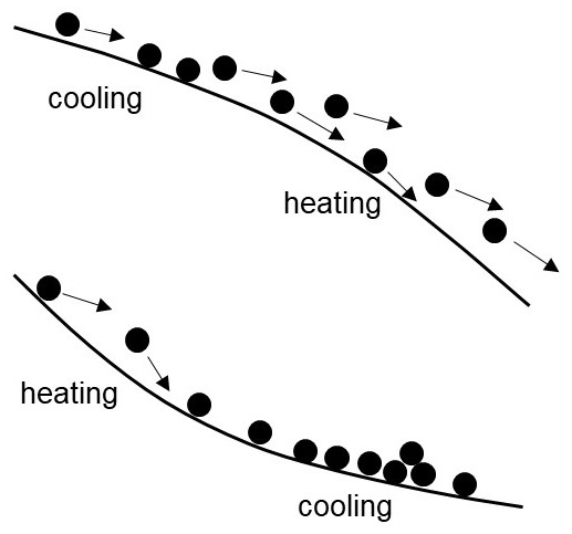
Figure 5 Cartoon of hillslope surfaces with downslope variations in steepness leading to concomitant variations in heating, cooling and deposition; this is in contrast to a planar slope with uniform μ that produces either net heating or net cooling, or isothermal conditions.

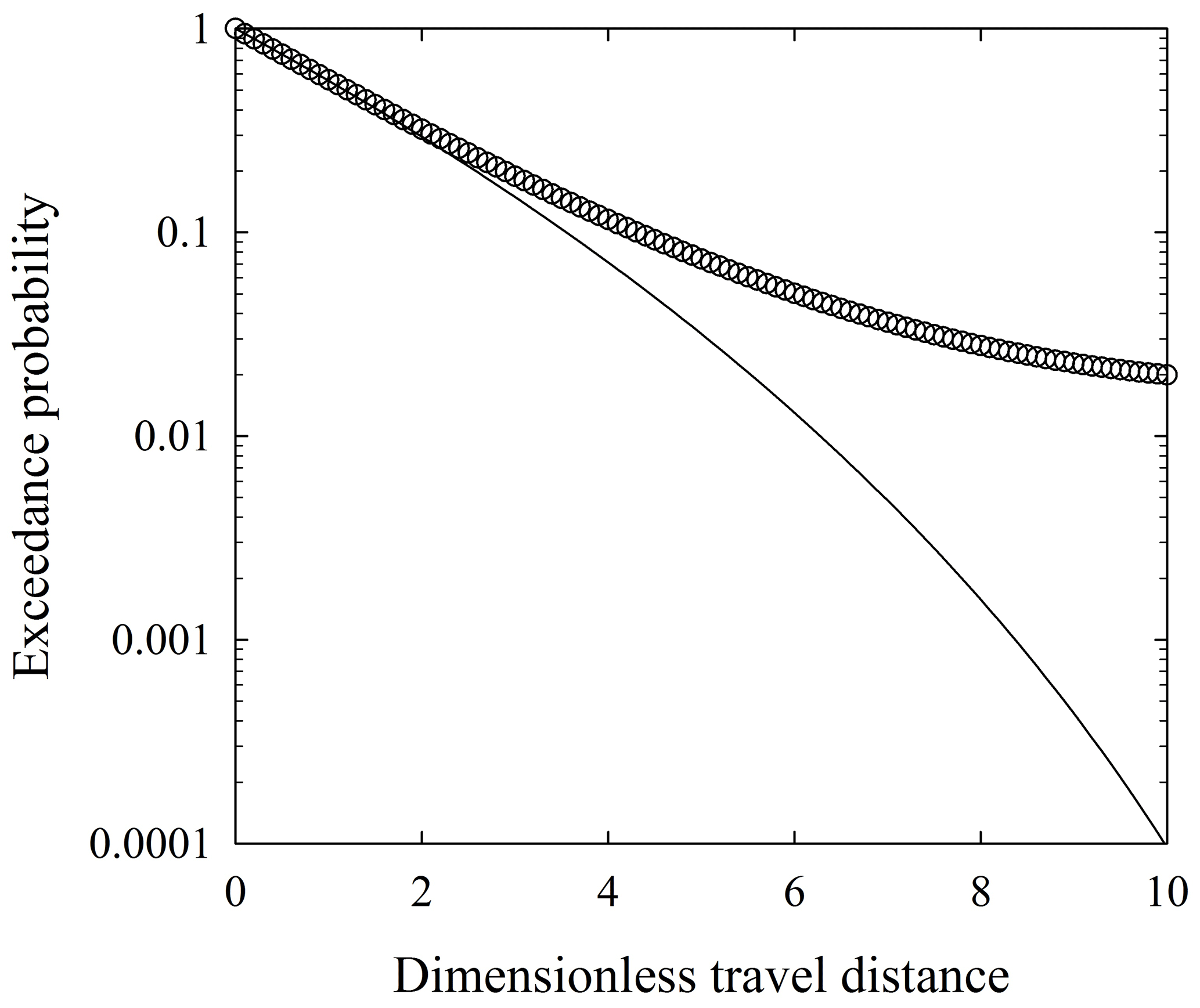
Figure 6 Plot of exceedance probability $R_{\widehat{x}}\left(\widehat{x}\right)$ versus dimensionless travel distance $\widehat{x}$ showing conditions with fixed net cooling (solid line) and conditions that start with the same cooling rate but then involve a decreasing rate with increasing distance $\widehat{x}$ (circles). In this example the Kirkby number starts at Ki=0.70 at $\widehat{x}=\mathrm{0}$ and increases to Ki=0.96 at $\widehat{x}=\mathrm{10}$.

In these examples we let α vary with the Kirkby number Ki according to Eq. (52) in anticipation of results presented in the companion paper. A decreasing rate of cooling associated with, for example, steepening in the downslope direction generally increases the heaviness of the tail of the distribution relative to the tail associated with a fixed rate of cooling (Fig. 6). We present evidence in the companion paper that this occurs in the field-based experiments reported by DiBiase et al. (2017). Specifically, particles were launched down a rough hillslope surface, and then their travel distances were measured over a 14 m interval. Particles reaching the steeper slope below the measurement interval continued to the base of the hillslope without stopping. In turn, an increasing rate of cooling (e.g., with decreasing slope in the downslope direction) generally lightens the tail and may lead to truncation of the distribution if the rate increases rapidly enough. Moreover, a condition involving initial heating followed by cooling (e.g., with a concave hillslope surface) can lead to a distribution with a finite mode (Fig. 7). These examples represent situations where particle travel distances cannot necessarily be approximated by a distribution whose parametric values are set by the hillslope conditions at the position where particle motions start. We defer further examination of this behavior, including use of the convolutions in Eqs. (5) and (6), for a later time.

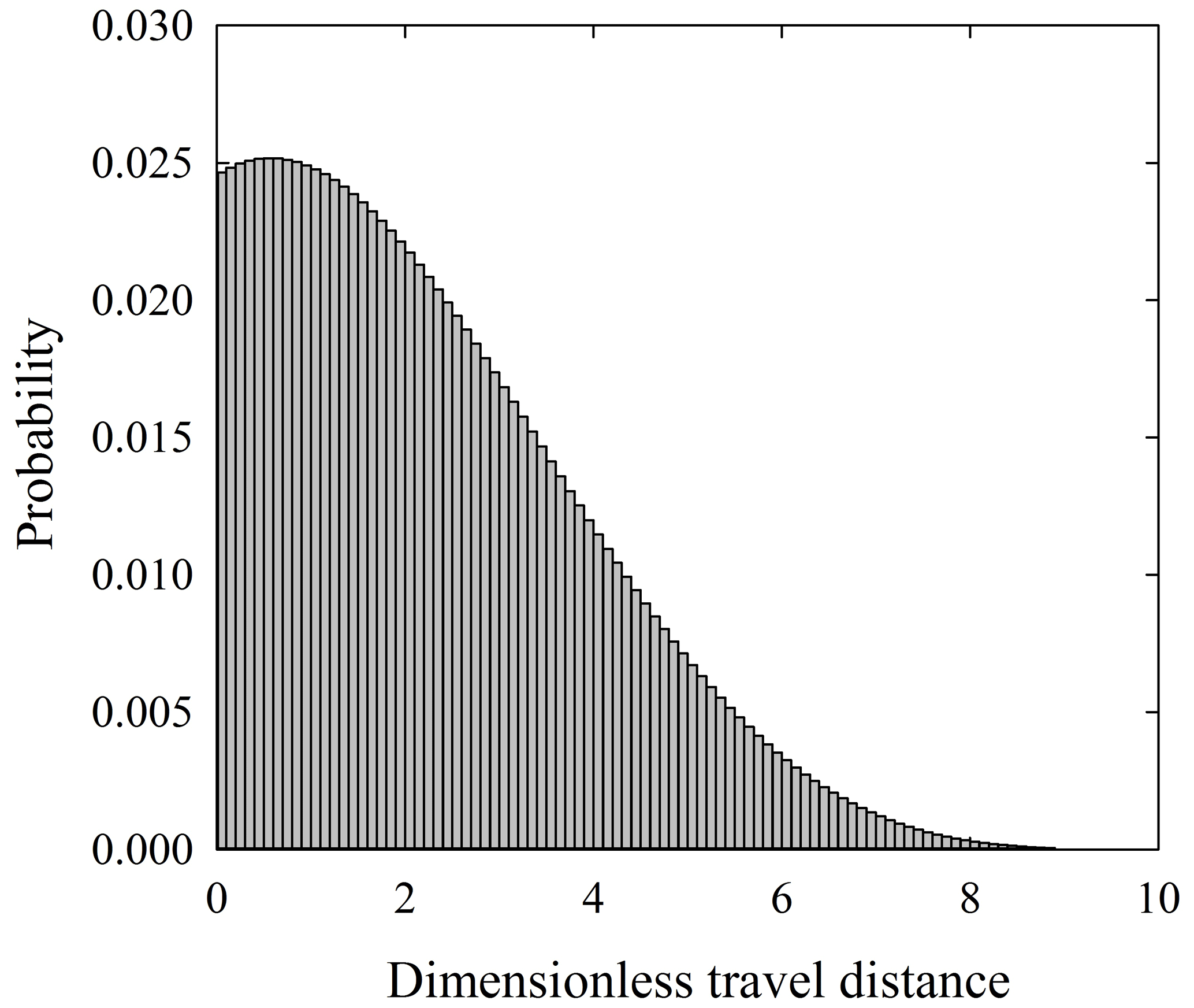
Figure 7 Probability mass function $f_k(k;\widehat{x})$ of discrete travel distances k associated with initial net heating over small k followed by net cooling with increasing k, leading to a finite mode. In this example the Kirkby number starts at Ki=0.90 at $k\mathrm{d}\widehat{r}=\widehat{x}=\mathrm{0}$ and decreases to Ki=0.57 at $k\mathrm{d}\widehat{r}=\widehat{x}=\mathrm{10}$.

7 Discussion and conclusions

Our formulation of rarefied particle motions is based on a description of the energy balance of a cohort of particles treated as a rarefied granular gas, as well as a description of particle deposition that depends on the energy state of the particles. The formulation leads to a generalized Pareto distribution of particle travel distances, Eq. (74). This distribution represents three well-defined behaviors in which the Kirkby number Ki – the ratio of gravitational heating to frictional cooling – has a principal role. Conditions with relatively small Ki lead to rapid thermal collapse such that the distribution of travel distances is bounded. For intermediate values of Ki the rate of gravitational heating may be matched by the rate of frictional cooling, giving approximately isothermal conditions and an exponential distribution of travel distances. Conditions with large Ki and net heating lead to a heavy-tailed distribution of travel distances. We provide compelling evidence of all three behaviors in our companion paper (Furbish et al., 2021a). Here we emphasize that we do not choose the generalized Pareto distribution in the empirical manner of selecting a distribution based on goodness-of-fit criteria applied to data sets. Rather, this distribution is dictated by the physics of the problem, just as, for example, the Boltzmann distribution (an exponential distribution) emerges in classical statistical mechanics from consideration of the accessible energy microstates of a gas system. We elaborate this point in the third companion paper (Furbish et al., 2021b).

Two of the most important elements of the formulation are the deposition length scales l_c(E_p) and L_c(E_h), the former being keyed to the specific particle energy state E_p and the latter being keyed to the harmonic average energy E_h of the particle cohort. Indeed, these lengths provide the essential connection between particle deposition and the energy balance of the particle cohort. We assume that l_c is set by the advective cooling length scale in the Fokker–Planck equation, that is, Eq. (44). This is a natural choice in that deposition must go with cooling. The energy-specific deposition rate in the absence of heating is then specified as if deposition proceeds as a spatial Poisson process. We emphasize that this represents a maximum (information) entropy choice in the sense that it is faithful to what we think we know, namely, the connection between deposition and cooling, as well as to what we do not know (Jaynes, 1957a, b), namely, any detailed physics that would produce a different rate (for example, involving a nonlinear dependence on energy state) but which cannot be specified or constrained with available information. This description then leads to the interesting result, Eq. (46), that the loss of total energy due to deposition appears to be independent of the energy state. In particular, the loss of large energy states occurs at a relatively slow rate, whereas the loss of small energy states occurs at a relatively fast rate. In effect the rate of loss of energy per energy interval is fixed across energy states. The result is that the energy E_p cancels with substitution of Eq. (45) into the integral in Eq. (46) such that the total loss becomes independent of the energy state. That is, the loss of total energy goes simply with the loss of particles (and the energy they possess).

In turn, the total deposition rate is energy dependent. This rate, defined by the length scale L_c, is obtained by integrating the number density of particles over all possible energy states as in Eq. (48). Because l_c is keyed to the energy state E_p, but the integral in Eq. (48) does not involve this energy in the numerator, the result involves the reciprocal of the harmonic average energy E_h. In general, the harmonic average diverges from the arithmetic average E_a with increasing variance of the distribution of energy states. With $E_{\mathrm{a}}/E_{\mathrm{h}}=\mathit{\gamma }$, the resulting ratio $\mathit{\gamma }/E_{\mathrm{a}}$ in Eq. (56) (with dimensionless form given by Eqs. 61 or 64) reflects an increasing proportion of lower-energy particles available for deposition, relative to this availability with γ→1. This effect is directly apparent in the expression of the mean travel distance, Eq. (69), associated with isothermal conditions.

Note that the formulation does not involve specifying a threshold energy for deposition. Such an idea is mechanically irrelevant. Whereas low-energy particles are on average more likely to become disentrained than are high-energy particles, a set of particles with precisely the same low energy will for probabilistic reasons not be disentrained simultaneously. Each particle experiences a unique set of conditions that disentrain it; because of this uniqueness of conditions a particle with energy below an arbitrarily assigned threshold can with finite probability be gravitationally reheated to a higher-energy state. For given particle and surface roughness conditions, the formulation treats this aspect of disentrainment as a probabilistic process. In effect, this aspect is incorporated into the deposition lengths l_c and L_c as these are related to the distribution of particle energy states and the probabilistically expected extraction of energy during collisions.

Frictional cooling is formulated in terms of extraction of translational kinetic energy associated with particle–surface collisions. This involves the random variable ${\mathit{\beta }}_x=-\mathrm{\Delta }{E}_{\mathrm{p}}/E_{\mathrm{p}}$ whose energy-specific average $\stackrel{\mathrm{‾}}{{\mathit{\beta }}_x}$ is the expected proportion of energy extracted from particles with energy E_p. In detail the change in energy ΔE_p may be partitioned between a frictional loss, any conversion of translational to rotational energy, and any apparent loss associated with downslope incident motion reflected to transverse motion during a glancing collision. Our treatment of the dissipation quantity β_x as a random variable does not distinguish the details involved in collisions. Yet these details may be important in terms of effects of different particle sizes and shapes, specifically the likelihood that the partitioning of energy losses differs between sizes or shapes. Herein the factor α modulating the length scale in Eq. (51) has a dualistic role. As incorporated in Eq. (51), this quantity represents the effect of heating, namely, to decrease the likelihood of deposition by decreasing the proportion of particles that cool to sufficiently low energies for deposition to occur – which translates to suppressing the disentrainment rate and increasing the length scale of deposition L_c. As incorporated in Eq. (53), this quantity modulates the frictional cooling described by μ∝〈β_x〉 to give an apparent decrease in friction associated with deposition.

Whereas particles that are small relative to the surface roughness texture are on average more likely to experience near-collinear collisions with surface bumps and be “captured” within divots and pockets, particles that are large relative to the roughness texture are less likely to experience direct collisions with, or strong deflections by, smaller surface bumps. In addition, large particles are more likely to experience conversion of their translational energy into rotational energy with less loss during collisions. In particular, large spherical particles are more likely to roll or spin with increased heating, and large spinning particles are less likely than are smaller particles to be frictionally cooled. These points are reflected in the laboratory experiments of Samson et al. (1998, 1999) (Appendix J), the laboratory experiments of Kirkby and Statham (1975), and the field experiments of DiBiase et al. (2017) and Roth et al. (2020) (see the second companion paper; Furbish et al., 2021a). This also implies that for a given slope angle and surface roughness, some particle sizes may experience net cooling while some sizes experience net heating (Roth et al., 2020), likely contributing to the size sorting observed on many talus and scree slopes (Kirkby and Statham, 1975; Statham, 1976; Luckman, 2013). We suspect the noticeable sorting in Fig. 1 is due to these effects.

The formulation readily accommodates the idea of a mixed distribution composed of different distributions associated with different particle sizes or mechanical behaviors. This amounts to forming a sum of distributions, each weighted in proportion to the size classes involved in transport. As with individual sizes, the formulation assumes rarefied conditions – that particles of different sizes do not interact during their downslope motions, or that such interactions negligibly influence the particle energy balance relative to particle–surface interactions. We provide an example in the second companion paper (Furbish et al., 2021a).

With rockfall and subsequent particle motions over talus and scree surfaces, the initial energy state E_a0 can be approximated in terms of the fall height (Kirkby and Statham, 1975). But this is a special situation in which the initial energy can be reasonably constrained. More generally, and with reference to the entrainment forms of the flux and the Exner equation, Eqs. (5) and (6), we are concerned with entrainment of particles from many if not all positions on a hillslope in relation to disturbances. This points to the idea that entrainment, if followed by long-distance motions, requires sufficient initial heating to keep particles moving downslope. This in turn echoes the conclusion of Doane et al. (2018) that correctly specifying the entrainment rate is a key part of implementing formulations of nonlocal transport and mass conservation. Because of the significance of sediment capacitors (e.g., vegetation) in trapping and storing sediment on hillslopes (Lamb et al., 2013; Doane, 2018), there is merit in clarifying the initial energetics of particles upon their release (i.e., entrainment) from storage. There also is a need to examine re-entrainment and transport associated with particle collisions, analogous to work on particle splash during eolian transport and the energetics of collective entrainment (Ancey et al., 2008) by collisions during bed load transport (Lee and Jerolmack, 2018).

That the energy and mass balances are expressed in the form of coupled differential equations opens the possibility of describing effects of varying disentrainment rates in response to changing downslope conditions in a manner intrinsic to particle-based treatments of transport (Tucker and Bradley, 2010), but not readily incorporated in previous probabilistic descriptions. Namely, if surface conditions change in the downslope direction, for example, giving net cooling followed by heating or vice versa (Fig. 5), then particles whose travel distances are large enough “see” this change and their behavior concomitantly changes. In this case the coupled equations of energy and mass in principle can be solved to accommodate these changing conditions. Interestingly, as differential (or finite difference) equations these have a local form, yet they intrinsically represent nonlocal behavior in that information concerning the energy state E_a and the mass N is cumulatively handed from one position to the next downslope. In turn, the forms of $R_r(r;x^{\prime })$ and $f_r(r;x^{\prime })$ associated with any position x^′ in the expressions of the flux and its divergence, Eqs. (5) and (6), must be based on information downslope from this position.

In this regard, here we offer further perspective on what is meant by local versus nonlocal transport on hillslopes. A transition of travel distances involving a distribution with a light tail to one with a heavy tail, as embodied in the generalized Pareto distribution, does not distinguish local from nonlocal transport. As fully explained in Furbish and Roering (2013) and in Furbish et al. (2017a), the convolutions in Eqs. (5) and (6) represent nonlocal transport regardless of the form of the probability density function f_r(r;x) and its associated exceedance probability function R_r(r;x). These scale-independent expressions are just specialized forms of the master equation used in probabilistic descriptions of particle motions over a remarkable range of scales (Einstein, 1905; von Smoluchowski, 1906; Chandrasekhar, 1943; Risken, 1984). Nonlocal transport is a physical thing and refers to the idea that attributes of particle motions used in defining the rheology, the flux or its divergence at a position x depend on conditions “far” from this position (e.g., Bocquet et al., 2009; Brantov and Bychenkov, 2013; Henann and Kamrin, 2013). In contrast, local transport is a mathematical thing, not a physical thing, and refers to the idea that under certain circumstances the convolution form of the master equation can be approximated such that the flux or its divergence has the form of a local mathematical expression – for example, a Fokker–Planck equation – whose terms involve conditions associated with the local position x. As alluded to above, a local expression can be formulated when the distribution f_r(r;x) has finite moments and is peaked near the origin (r=0). A heavy-tailed behavior means that this is not justified. Rather, the full convolution or a fractional derivative approximation of it must be used (Schumer et al., 2009). Because of the generality and scale independence embodied in the master equation and the convolutions in Eqs. (5) and (6), the use of “nonlocal” as a qualifier of “transport” in reference to hillslopes actually is redundant (Doane, 2018). Its use is merely a reminder that the flux or its divergence at a position x depends on things happening upslope.

The entrainment rate E_s(x), the exceedance probability function R(r;x) and the distribution of travel distances f_r(r;x) within the integrals in Eqs. (5) and (6) are treated as continuous functions. However, this does not imply a continuum behavior. Like the Fokker–Planck equation, which describes the evolution of the probability density function of a random variable that may or may not satisfy the continuum hypothesis (see Appendix A in Furbish et al., 2018b), the continuous forms of Eqs. (5) and (6) represent a probabilistic description of expected behavior, not necessarily the behavior of any one realization (system). In practical terms, imagine a rockfall event from a cliff face involving an individual particle or a relatively small number of particles whose subsequent downslope motions then start at position x=0 at the base of the cliff. Inasmuch as the generalized Pareto distribution f_x(x) provides the correct description of the expected behavior of the particles from the rockfall event, then these particles may be viewed as a (small) sample drawn from this distribution. The outcome of each realization (sample) is almost certainly different from all other realizations. Over a period of time the pooled outcomes (travel distances) of many events converge to the smooth representations given by f_x(x) and R_x(x) – as if Gabet and Mendoza (2012), DiBiase et al. (2017) and Roth et al. (2020) had performed a gazillion additional rock-launching experiments (see second companion paper, Furbish et al. 2021a) and then pooled the outcomes of these experiments. Implications of this idea are examined further in Furbish and Haff (2010), Furbish and Roering (2013), and Furbish et al. (2017b, 2018b), and again in the fourth companion paper (Furbish and Doane, 2021).

The formulation may have interesting implications for examining Martian landforms. For example, the appearance of the acceleration g in Eqs. (51), (56) and (83) immediately suggests the possibility that particle travel distances are on average significantly longer on Mars than on Earth for otherwise similar particle sizes and surface-roughness conditions; we are confident in suggesting that future Martians likely will have far more fun than Earthlings in the sport of boulder rolling, notably on the crater rim of Olympus Mons. Nonetheless, we leave it to folks more familiar with Mars than we are to examine this. A key element of doing this is to either assume that the friction factor μ is similar to what occurs on Earth (which may be entirely reasonable) or further unfold the elements of this factor. We comment on this idea again in the second companion paper (Furbish et al., 2021a). We meanwhile note that a similar question arises in relation to the role of g in setting the friction of granular slopes on Mars. Atwood-Stone and McEwen (2013) address this question by examining dune slip-face angles on Mars and suggest that the similarity of these angles with those observed on Earth weakens any argument for different granular behavior associated with g – consistent with independent assessments (Moore et al., 1987; Tesson et al., 2020) and the idea that this angle is set by the static granular force-chain network (Cates et al., 1998; Furbish et al., 2008).

Appendix A: Choice of terminology

The study of granular materials is concerned with the behavior of the phases of these materials and associated phase transitions (Jaeger et al., 1996; Baldassarri et al., 2005; Daniels and Behringer, 2006; Forterre and Pouliquen, 2008; Jerolmack and Daniels, 2019). These phases and transitions share attributes with ordinary materials – solids, liquids and gases – although granular materials often exhibit behavior that is much different than ordinary materials. Nonetheless, it has become customary in the study of granular materials to adopt terminology similar to that used to describe ordinary materials.

The ideas of heating and cooling of a granular material are straightforward, to mean a change in the granular temperature of the material, specifically the average translational kinetic energy of the particles (but see van Zon and MacKintosh, 2004, and Baldassarri et al., 2005). However, granular materials do not possess an internal energy in the sense that we attribute to the particles of an ordinary liquid or gas. This means that heating of a granular material requires a mechanical input of energy, whereas cooling is associated with dissipative (non-conservative) collisions of particles with each other and with boundaries. In the problem at hand, gravitational heating occurs as particles move downslope, and their gravitational potential energy is converted to kinetic energy. Frictional cooling is associated with dissipative particle–surface interactions (e.g., collisions).

The ideas of melting and freezing of a granular material (Daniels and Behringer, 2006) pertain to the transition between a solid-like phase and a hydrodynamic (fluid-like) phase. However, in the problem at hand, we are concerned with rarefied particle conditions in which disentrainment from the rarefied state to the solid-like state or vice versa does not involve an intermediate hydrodynamic phase (e.g., Haff, 1983; Jenkins and Savage, 1983; Jaeger et al., 1996). Entrainment is akin to sublimation, and disentrainment is akin to deposition (or desublimation). Phase transitions involving an intermediate hydrodynamic phase (evaporation–condensation and melting–freezing) are represented in Earth-surface processes, for example, by melting (entrainment) and freezing (disentrainment) at the base of a granular flow, dry or wet. We recommend the papers by Forterre and Pouliquen (2008), Frey and Church (2011), Houssais et al. (2015), and Jerolmack and Daniels (2019) for perspectives on this emerging topic, notably in relation to transport by shear flows.

Appendix B: Particle cohort

In order to clarify the idea of a cohort of particles associated with a control volume with edge length dx (Fig. 2), here we offer a straightforward thought experiment. As a point of reference, the study of granular gases typically involves consideration of the behavior of an individual system composed of many particles that are mechanically heated, where energy dissipation is associated with particle–particle collisions. In contrast, our problem involves an unusual situation in that we must start by considering a system composed of one particle, where energy dissipation occurs with particle–surface collisions, and then in turn consider the behavior of an ensemble of such systems.

Imagine a box containing one particle. We mechanically shake the box and the particle is heated. At any instant the particle has kinetic energy E_p. Each time the particle collides with the floor of the box it is re-heated, and each time it collides with a wall of the box energy is extracted. Eventually the particle by chance has sufficiently low energy that when it next encounters a wall it becomes irreversibly deposited (disentrained) onto the wall. Then the box has no moving particle.

Like Gibbs (1902), we now imagine a great number N of nominally identical but independent single-particle systems, where each particle in each system (box) behaves according to the same laws of physics, each undergoing heating and collisional cooling, and occasionally being deposited (Fig. B1). We now choose one instant in time and examine the state of each particle. Some particles previously have been deposited, so at this instant N refers to those systems whose particles are in motion. At this instant each particle has kinetic energy E_p, and we may define the ensemble probability density $f_{E_{\mathrm{p}}}\left(E_{\mathrm{p}}\right)$ of energy states E_p. As a consequence we also may at this instant define the ensemble-averaged kinetic energy 〈E_p〉 and the total energy E=N〈E_p〉. (Alternatively, we could imagine all N particles in a single box at one instant, but with the caveat that we must imagine them as not interacting with each other, only with the floor and walls of the box.) We now choose a successive instant in time, namely, t+dt. During dt the number N decreased with deposition of some particles, the distribution $f_{E_{\mathrm{p}}}\left(E_{\mathrm{p}}\right)$ changed, and the average energy 〈E_p〉 and the total energy E changed.

Figure B1 Schematic diagram of surface inclined at angle θ and control volume with edge length dx through which particles move, with Gibbs-like ensemble of single-particle systems leading to definition of the cohort of N(x) particles starting at the left face of the control volume.

More generally we can choose N different instants in time t, one instant for each box, and examine the state of each particle. Then, upon collecting the particles as a cohort independently of the selected times, like above we observe an ensemble distribution of energy states with specific average energy 〈E_p〉 and total energy E. At this point we relax the idea of a box and simply view particle–wall collisions more generally as particle–surface collisions during motions parallel to x; instead of heating the particles via particle–floor collisions we imagine this to occur continuously by gravitational heating. We then let the N selected instants in time coincide with those instants that each of the particles is located at a specified position x. That is, these are the N(x) particles located at the left face of the interval x to x+dx (Fig. B1). We may then examine how the number N(x) and the ensemble distribution $f_{E_{\mathrm{p}}}(E_{\mathrm{p}},x)$ and its moments change over the interval x to x+dx as this particle cohort moves downslope. Note that each member of the cohort not deposited within this interval may arrive at position x+dx at a different instant in time. This is unimportant, however, as we are interested only in how the energy states of the particles vary with position x. Similarly, upon choosing any subsequent downslope position x, we must recognize that the N(x) particles reaching this position do so at entirely different instants in time. Here is a final note: in this problem a particle ensemble average is identical to a Gibbs ensemble average.

Consider, then, both similarities and differences between conditions in a “normal” non-equilibrium granular gas and the rarefied conditions of particle motions on hillslopes. As a reminder, the rarefied conditions that we describe do not involve particle–particle collisions, only particle–surface collisions. The Knudsen number in any realization is effectively infinite. As described in the text, the distribution $n_{E_{\mathrm{p}}}(E_{\mathrm{p}},x)$ of energy states E_p of the particle cohort (ensemble) varies with position x. Because the moments of this distribution are assumed to be defined, we could in fact also define the distribution of downslope velocities, thence the mean velocity and fluctuations about the mean. That is, we could formally define a granular temperature (Goldhirsch, 2008) and then associate this temperature with an internal granular energy content at any position x. However, the granular temperature thus defined for the rarefied problem is not physically relevant to this problem, and a granular internal energy does not physically exist. Indeed, granular energy is neither advected nor diffused in the sense of a normal granular gas system, for example, a granular flow. Moreover, quantities such as the granular density and pressure do not exist. In short, there are no “internal” gas dynamics whatsoever, as the rarefied conditions do not represent a particle system that evolves dynamically over time and space, as with a granular gas in a box or in a conduit or over an inclined surface, each of which involves dissipative particle–particle collisions during the gas evolution. Yet the description of the spatial evolution of the distribution of the energy states of the particle ensemble remains entirely relevant. Indeed, the rarefied case examined herein represents a highly unusual granular gas. To our knowledge this particular granular gas problem has not been examined before. The closest direct analogue seems to be that reported by Almazán et al. (2017), who, building from the work of Volfson et al. (2006), show that the formalism used in describing the cooling and thermal collapse of a granular gas is akin to the formalism used in describing the dissipative energetics of a single nonelastic ball bouncing on a smooth horizontal surface (without energy input from vibration or gravitational heating).

Whereas the dynamics of an ordinary granular gas are centered on dissipative particle–particle collisions, in our problem the dynamics are centered on dissipative particle–surface collisions. This dynamic is fundamentally a boundary-related phenomenon, not an internal one. In a standard granular gas, energy dissipation occurs during particle–particle collisions. But note that, whereas a dissipative collision between two particles generally leads to an overall loss of kinetic energy, the kinetic energy of one of the two particles may actually increase. In contrast, in our problem involving only particle–surface collisions, essentially all collisions involve extraction (dissipation) of the particle kinetic energy defined with respect to downslope motion. Thus, all collisions are “cooling” in the sense of reducing particle kinetic energy. Similarly, gravity provides a uniform “heating” in the sense of increasing kinetic energy. Thus, we appeal to the ideas of cooling and heating without reference to fluctuating motions (and granular temperature), where cooling simply refers to the idea that kinetic energy is extracted from the particle cohort via collisional friction and heating refers to the idea that kinetic energy is added to the cohort via conversion of gravitational potential energy into kinetic form. The idea of thermal collapse then is entirely satisfactory (e.g., Volfson et al., 2006). We further reemphasize that our formulation involves the evolution of $n_{E_{\mathrm{p}}}(E_{\mathrm{p}},x)$ with respect to space, whereas standard granular gas theory typically involves hydrodynamic-like descriptions of quantities such as the granular density, temperature, pressure and velocity that evolve with respect to time (in an Eulerian manner), where it is assumed that local continuum-like definitions of these quantities exist (e.g., Goldhirsch, 2008) – conditions that are not relevant in the rarefied problem that we examine.

Appendix C: The Fokker–Planck-like equation

Let $q=E_{\mathrm{p}}(x+\mathrm{d}x)-E_{\mathrm{p}}\left(x\right)$ denote a change in the energy of a particle over the small distance dx, and let $f_q(q;E_{\mathrm{p}},x)$ denote the probability density function of the changes q associated with the energy state E_p and position x. If $n_{E_{\mathrm{p}}}(E_{\mathrm{p}},x)$ denotes the number density of particle energies E_p, then according to the master equation,

$$\begin{array}{}\text{(C1)}& \begin{array}{rl}{n}_{E_{\mathrm{p}}}& \left(E_{\mathrm{p}},x+\mathrm{d}x\right)\\ & =\underset{\mathrm{0}}{\overset{\mathrm{\infty }}{\int }}{f}_q\left(q;E_{\mathrm{p}}-q,x\right)n_{E_{\mathrm{p}}}\left(E_{\mathrm{p}}-q,x\right)\mathrm{d}q.\end{array}\end{array}$$

Assuming the density $f_q(q;E_{\mathrm{p}},x)$ is peaked near q=0 with finite first and second moments, we may expand the integrand in Eq. (C1) as a Taylor series to second order, subtract $n_{E_{\mathrm{p}}}(E_{\mathrm{p}},x)$ from both sides, then divide by dx and take the limit as dx→0 to obtain a Fokker–Planck-like equation, namely,

$$\begin{array}{}\text{(C2)}& \begin{array}{rl}{\displaystyle \frac{\partial n_{E_{\mathrm{p}}}\left(E_{\mathrm{p}},x\right)}{\partial x}}& =-{\displaystyle \frac{\partial }{\partial E_{\mathrm{p}}}}\left[k_{\mathrm{1}}\left(E_{\mathrm{p}},x\right)n_{E_{\mathrm{p}}}\left(E_{\mathrm{p}},x\right)\right]\\ & +{\displaystyle \frac{\mathrm{1}}{\mathrm{2}}}{\displaystyle \frac{{\partial }^{\mathrm{2}}}{\partial E_{\mathrm{p}}^{\mathrm{2}}}}\left[k_{\mathrm{2}\mathrm{c}}\left(E_{\mathrm{p}},x\right)n_{E_{\mathrm{p}}}\left(E_{\mathrm{p}},x\right)\right].\end{array}\end{array}$$

Here, k₁(E_p,x) is a drift speed and k_2c(E_p,x) is a diffusion coefficient defined by

$$\begin{array}{}\text{(C3)}& k_{\mathrm{1}}\left(E_{\mathrm{p}},x\right)=\underset{\mathrm{d}x\to \mathrm{0}}{lim}{\displaystyle \frac{\mathrm{1}}{\mathrm{d}x}}\underset{-\mathrm{\infty }}{\overset{\mathrm{\infty }}{\int }}q{f}_q\left(q;E_{\mathrm{p}},x\right)\mathrm{d}q\end{array}$$

and

$$\begin{array}{}\text{(C4)}& k_{\mathrm{2}\mathrm{c}}\left(E_{\mathrm{p}},x\right)=\underset{\mathrm{d}x\to \mathrm{0}}{lim}{\displaystyle \frac{\mathrm{1}}{\mathrm{d}x}}\underset{-\mathrm{\infty }}{\overset{\mathrm{\infty }}{\int }}{q}^{\mathrm{2}}{f}_q\left(q;E_{\mathrm{p}},x\right)\mathrm{d}{E}_{\mathrm{p}}.\end{array}$$

The drift speed k₁(E_p,x) has two parts: one associated with gravitational heating and one associated with frictional cooling. Starting with gravitational heating, let h(x) denote the height of a particle within the gravitational field at position x. If E_p(x) denotes the particle kinetic energy equal in magnitude to the potential energy mgh(x) at height h(x), then $E_{\mathrm{p}}(x+\mathrm{d}x)=mgh(x+\mathrm{d}x)$ is the magnitude of the particle kinetic energy at the height h(x+dx), assuming a complete conversion of gravitational to kinetic energy without loss. Thus,

$$\begin{array}{}\text{(C5)}& q=mg\left[h\right(x+\mathrm{d}x)-h(x\left)\right].\end{array}$$

This indicates that q in Eq. (C3) is independent of the energy state E_p and therefore may be removed from the integral. We thus write Eq. (C3) as

$$\begin{array}{}\text{(C6)}& \begin{array}{rl}{k}_{\mathrm{1}\mathrm{h}}& =mg\underset{\mathrm{d}x\to \mathrm{0}}{lim}{\displaystyle \frac{h(x+\mathrm{d}x)-h\left(x\right)}{\mathrm{d}x}}\underset{-\mathrm{\infty }}{\overset{\mathrm{\infty }}{\int }}{f}_q\left(q;E_{\mathrm{p}},x\right)\mathrm{d}q\\ & =mg{\displaystyle \frac{\mathrm{d}h}{\mathrm{d}x}}=mg\sin \mathit{\theta }.\end{array}\end{array}$$

This is the steady rate of gravitational heating.

The part of k₁(E_p,x) associated with frictional cooling is obtained as follows. With particle–surface collisions we may assume that q is proportional to the expected value of ΔE_p. In turn we let $n_x=\mathrm{1}/\mathit{\lambda }$ denote the expected number of collisions per unit distance, where λ is the expected travel distance between collisions. This leads to

$$\begin{array}{}\text{(C7)}& k_{\mathrm{1}\mathrm{c}}\left(E_{\mathrm{p}},x\right)={\displaystyle \frac{\mathrm{d}\stackrel{\mathrm{‾}}{q}}{\mathrm{d}x}}\approx n_x\stackrel{\mathrm{‾}}{\mathrm{\Delta }{E}_{\mathrm{p}}}=n_x\stackrel{\mathrm{‾}}{{\mathit{\beta }}_x}{E}_{\mathrm{p}},\end{array}$$

where the overline denotes an average over particles at the energy state E_p (rather than a global average).

Because gravitational heating is a fixed quantity according to Eq. (C6), heating does not involve diffusion. In turn, the diffusion coefficient k_2c(E_p,x) associated with frictional cooling is given by

$$\begin{array}{}\text{(C8)}& k_{\mathrm{2}\mathrm{c}}\left(E_{\mathrm{p}},x\right)={\displaystyle \frac{\mathrm{d}\stackrel{\mathrm{‾}}{q^{\mathrm{2}}}}{\mathrm{d}x}}\approx n_x\stackrel{\mathrm{‾}}{{\left(\mathrm{\Delta }{E}_{\mathrm{p}}\right)}^{\mathrm{2}}}=n_x\stackrel{\mathrm{‾}}{{\mathit{\beta }}_x^{\mathrm{2}}}{E}_{\mathrm{p}}^{\mathrm{2}}.\end{array}$$

Note that whereas k_1h is a fixed quantity, k_1c and k_2c must be viewed as statistically expected quantities.

Appendix D: Expected travel distance between collisions

Momentarily let $v=\langle u^{\mathrm{2}}{\rangle }^{\mathrm{1}/\mathrm{2}}$, and then let v₀ denote the surface-parallel velocity of a particle rebounding with reflection angle ϕ measured from the surface (Fig. D1). We then know that

$$\begin{array}{}\text{(D1)}& U_{\mathrm{0}}=v_{\mathrm{0}}{\displaystyle \frac{\cos (\mathit{\varphi }-\mathit{\theta })}{\cos \mathit{\varphi }}}\mathrm{and}{W}_{\mathrm{0}}=v_{\mathrm{0}}{\displaystyle \frac{\sin (\mathit{\varphi }-\mathit{\theta })}{\cos \mathit{\varphi }}},\end{array}$$

where U₀ denotes the horizontal velocity and W₀ denotes the vertical velocity. For a vertical change in elevation Z over a horizontal distance X associated with the surface-parallel distance λ, we know that $Z=-SX=-S{U}_{\mathrm{0}}{t}_{\mathrm{0}}$, where t₀ is the travel time. For a rebounding particle starting at position z₀=0 we may deduce from Newton's second law that

$$\begin{array}{}\text{(D2)}& Z=-S{U}_{\mathrm{0}}{t}_{\mathrm{0}}=-{\displaystyle \frac{\mathrm{1}}{\mathrm{2}}}g{t}_{\mathrm{0}}^{\mathrm{2}}+W_{\mathrm{0}}{t}_{\mathrm{0}},\end{array}$$

which gives

$$\begin{array}{}\text{(D3)}& t_{\mathrm{0}}={\displaystyle \frac{\mathrm{2}{W}_{\mathrm{0}}}{g}}+{\displaystyle \frac{\mathrm{2}S{U}_{\mathrm{0}}}{g}}.\end{array}$$

With $\mathit{\lambda }=X/\cos \mathit{\theta }=U_{\mathrm{0}}{t}_{\mathrm{0}}/\cos \mathit{\theta }$, we then combine Eqs. (D1)–(D3) to obtain

$$\begin{array}{}\text{(D4)}& \mathit{\lambda }={\displaystyle \frac{\mathrm{2}{v}_{\mathrm{0}}^{\mathrm{2}}\sin (\mathit{\varphi }-\mathit{\theta })\cos (\mathit{\varphi }-\mathit{\theta })}{g{\cos }^{\mathrm{2}}\mathit{\varphi }\cos \mathit{\theta }}}+{\displaystyle \frac{\mathrm{2}S{v}_{\mathrm{0}}^{\mathrm{2}}{\cos }^{\mathrm{2}}(\mathit{\varphi }-\mathit{\theta })}{g{\cos }^{\mathrm{2}}\mathit{\varphi }\cos \mathit{\theta }}}.\end{array}$$

Upon expanding sin (ϕ−θ) and cos (ϕ−θ) using difference formulae, algebra and trigonometric identities eventually lead to

$$\begin{array}{}\text{(D5)}& \mathit{\lambda }={\displaystyle \frac{\mathrm{2}{v}_{\mathrm{0}}^{\mathrm{2}}\cos \mathit{\theta }}{g}}\tan \mathit{\varphi }\left(\mathrm{1}+\tan \mathit{\varphi }\tan \mathit{\theta }+{\tan }^{\mathrm{2}}\mathit{\theta }+\tan \mathit{\varphi }{\tan }^{\mathrm{3}}\mathit{\theta }\right).\end{array}$$

For θ=0, this reduces to $\mathit{\lambda }=\mathrm{2}{v}_{\mathrm{0}}^{\mathrm{2}}\tan \mathit{\varphi }/g$. If for small slopes tan ϕ∼tan θ and for large slopes tan ϕ≪tan θ, then at leading order,

$$\begin{array}{}\text{(D6)}& \mathit{\lambda }\approx {\displaystyle \frac{\mathrm{2}{v}_{\mathrm{0}}^{\mathrm{2}}\cos \mathit{\theta }}{g}}\tan \mathit{\varphi }\left(\mathrm{1}+{\tan }^{\mathrm{2}}\mathit{\theta }\right)={\displaystyle \frac{\mathrm{2}{v}_{\mathrm{0}}^{\mathrm{2}}\tan \mathit{\varphi }}{g\cos \mathit{\theta }}}.\end{array}$$

For the purpose of scaling, we now assume that $v_{\mathrm{0}}^{\mathrm{2}}\sim \langle u^{\mathrm{2}}\rangle$ and write

$$\begin{array}{}\text{(D7)}& \mathit{\lambda }\approx {\displaystyle \frac{\mathrm{2}\langle u^{\mathrm{2}}\rangle \tan \mathit{\varphi }}{g\cos \mathit{\theta }}},\end{array}$$

which gives Eq. (26) in the text. The soft matter trajectory analysis of Tajima and Fujisawa (2020) includes viscous air resistance, which we neglect.

Figure D1 Definition diagram for determining travel distance λ.

Appendix E: Energy extraction during collisions

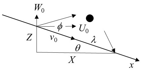
Here we provide a qualitative description of the basis for assuming that a change in the downslope energy of a particle associated with a collision can be expressed as $\mathrm{\Delta }{E}_{\mathrm{p}}=-{\mathit{\beta }}_x{E}_{\mathrm{p}}$ wherein both β_x and ΔE_p must be treated as random variables. We start by noting that the topic of particle collision mechanics is well developed for idealized particle–particle collisions and particle–surface collisions involving spherical particles, as well as peculiarities of non-collinear collisions associated with irregular particles. Relevant elements are covered in Brach (1984, 1989, 1991), Stronge (1990, 2000), Brach and Dunn (1992, 1995), and Ismail and Stronge (2008). Although we cannot directly apply details of this work given the complexity of particle motions on natural rough hillslopes, this work nonetheless offers a clear guide in the interpretation of the relation $\mathrm{\Delta }{E}_{\mathrm{p}}=-{\mathit{\beta }}_x{E}_{\mathrm{p}}$, notably in relation to experimental results presented in the second companion paper (Furbish et al., 2021a).

With reference to Fig. E1, consider an idealized collision of a spherical particle with a rigid planar surface with slope angle θ. Let u, w and ω respectively denote the surface parallel velocity, the surface normal velocity and the angular velocity of the particle with mass m and radius $r=D/\mathrm{2}$, and let the subscripts 1 and 2 denote incident and reflection values. With appropriate modification of the coordinate and sign convention used by Brach (1991), the momentum components associated with impulses can be expressed as (Brach, 1991, 1998; Brach and Dunn, 1995)

$$\begin{array}{}\text{(E1)}& {\displaystyle }& {\displaystyle }{w}_{\mathrm{2}}=-\mathit{ϵ}{w}_{\mathrm{1}},\text{(E2)}& {\displaystyle }& {\displaystyle }{u}_{\mathrm{2}}=u_{\mathrm{1}}+{\mathit{\mu }}_c(\mathrm{1}+\mathit{ϵ})w_{\mathrm{1}}+g\mathit{\tau }\left(\sin \mathit{\theta }-{\mathit{\mu }}_c\cos \mathit{\theta }\right)\mathrm{and}\text{(E3)}& {\displaystyle }& {\displaystyle }{\mathit{\omega }}_{\mathrm{2}}={\mathit{\omega }}_{\mathrm{1}}+{\displaystyle \frac{\mathrm{5}}{\mathrm{2}}}{\displaystyle \frac{{\mathit{\mu }}_c}{r}}\left[(\mathrm{1}+\mathit{ϵ})w_{\mathrm{1}}-g\mathit{\tau }\cos \mathit{\theta }\right],\end{array}$$

where w₁<0, ϵ is the normal coefficient of restitution attributed to Newton, μ_c is the ratio of tangential to normal impulses during the collision, and τ is the impulse duration. Note that μ_c generally is not a coefficient of friction, although it may be equal to a coefficient of friction in special cases, for example, with sliding throughout the entire duration of the collision (Brach, 1991; Brach and Dunn, 1992). Also note that μ_c=0 if u₁=0.

Figure E1 Definition diagram for idealized collision of a spherical particle with a rigid planar surface.

The second term on the right side of Eq. (E2) represents the effect of tangential friction on the velocity u, increasing with the magnitude of the normal impulse associated with the velocity w₁. This term may be considered the dynamic contribution to friction during τ. The term gτsin θ represents the downslope contribution to the impulse associated with the weight of the particle, and the term gτμ_ccos θ represents an enhancement of friction associated with this weight. The impulse duration τ may be on the order of milliseconds for a hard particle impacting a hard surface. It may be longer for a hard particle impacting a relatively soft surface (Brach, 1991). If the magnitude of w₁ is sufficiently large and τ is sufficiently short, the gravitational terms in Eqs. (E2) and (E3) may be neglected. The second term on the right side of Eq. (E3) represents the effect of tangential friction in contributing to rotational motion, that is, the conversion of translational energy to rotational energy.

Collisions involving small incident angles begin with sliding during the impulse duration τ. If with a sufficient normal dynamic force this initial sliding gives way to stick prior to separation, then for a sphere with moment of inertia $I=(\mathrm{2}/\mathrm{5})m{r}^{\mathrm{2}}$, the velocity u₂=rω₂ at separation. This leads to

$$\begin{array}{}\text{(E4)}& u_{\mathrm{2}}={\displaystyle \frac{u_{\mathrm{1}}+g\mathit{\tau }\sin \mathit{\theta }}{\mathrm{1}+\mathrm{2}/\mathrm{5}}},\end{array}$$

which represents the outcome of a conversion of translational to rotational motion with stick. Whereas the resultant velocity u₂ can be determined in this situation, the effect of sliding on u₂ cannot be analytically constrained. Nonetheless, Eq. (E3) indicates that collisions induce a conversion of translational to rotational motion in that tangential friction during an impulse exerts a torque on the particle, thereby extracting translational kinetic energy that is in addition to work performed during particle deformation and by friction. We also note that low-angle collisions likely dominate in the problem at hand.

In order to recast the problem in terms of kinetic energy, we start by squaring Eqs. (E1)–(E3) to give

$$\begin{array}{}\text{(E5)}& {\displaystyle }{w}_{\mathrm{2}}^{\mathrm{2}}={\mathit{ϵ}}^{\mathrm{2}}{w}_{\mathrm{1}}^{\mathrm{2}},\text{(E6)}& {\displaystyle }\begin{array}{rl}{u}_{\mathrm{2}}^{\mathrm{2}}& =u_{\mathrm{1}}^{\mathrm{2}}+\mathrm{2}{\mathit{\mu }}_{\mathrm{c}}(\mathrm{1}+\mathit{ϵ})u_{\mathrm{1}}{w}_{\mathrm{1}}+u_{\mathrm{c}}^{\mathrm{2}}(\mathrm{1}+\mathit{ϵ}{)}^{\mathrm{2}}{w}_{\mathrm{1}}^{\mathrm{2}}\\ & +\mathrm{2}g\mathit{\tau }\left(\sin \mathit{\theta }-{\mathit{\mu }}_{\mathrm{c}}\cos \mathit{\theta }\right)u_{\mathrm{1}}\\ & +\mathrm{2}{\mathit{\mu }}_{\mathrm{c}}(\mathrm{1}+\mathit{ϵ})g\mathit{\tau }\left(\sin \mathit{\theta }-{\mathit{\mu }}_{\mathrm{c}}\cos \mathit{\theta }\right)w_{\mathrm{1}}\\ & +g^{\mathrm{2}}{\mathit{\tau }}^{\mathrm{2}}\left(\sin \mathit{\theta }-{\mathit{\mu }}_{\mathrm{c}}\cos \mathit{\theta }\right)\mathrm{and}\end{array}\text{(E7)}& {\displaystyle }\begin{array}{rl}{\mathit{\omega }}_{\mathrm{2}}^{\mathrm{2}}& ={\mathit{\omega }}_{\mathrm{1}}^{\mathrm{2}}+\mathrm{5}{\displaystyle \frac{{\mathit{\mu }}_{\mathrm{c}}}{r}}(\mathrm{1}+\mathit{ϵ}){\mathit{\omega }}_{\mathrm{1}}{w}_{\mathrm{1}}+{\displaystyle \frac{\mathrm{25}}{\mathrm{4}}}{\displaystyle \frac{{\mathit{\mu }}_{\mathrm{c}}^{\mathrm{2}}}{r^{\mathrm{2}}}}(\mathrm{1}+\mathit{ϵ}{)}^{\mathrm{2}}{w}_{\mathrm{1}}^{\mathrm{2}}\\ & -\mathrm{5}{\displaystyle \frac{{\mathit{\mu }}_{\mathrm{c}}}{r}}g\mathit{\tau }\cos \mathit{\theta }{\mathit{\omega }}_{\mathrm{1}}-{\displaystyle \frac{\mathrm{25}}{\mathrm{2}}}{\displaystyle \frac{{\mathit{\mu }}_{\mathrm{c}}^{\mathrm{2}}}{r^{\mathrm{2}}}}g\mathit{\tau }\cos \mathit{\theta }{w}_{\mathrm{1}}\\ & +{\displaystyle \frac{\mathrm{25}}{\mathrm{4}}}{\displaystyle \frac{{\mathit{\mu }}_{\mathrm{c}}^{\mathrm{2}}}{r^{\mathrm{2}}}}{g}^{\mathrm{2}}{\mathit{\tau }}^{\mathrm{2}}{\cos }^{\mathrm{2}}\mathit{\theta }.\end{array}\end{array}$$

In addition we square Eq. (E4) to give

$$\begin{array}{}\text{(E8)}& u_{\mathrm{2}}^{\mathrm{2}}={\displaystyle \frac{\mathrm{25}}{\mathrm{49}}}{u}_{\mathrm{1}}^{\mathrm{2}}+{\displaystyle \frac{\mathrm{50}}{\mathrm{49}}}g\mathit{\tau }\sin \mathit{\theta }{u}_{\mathrm{1}}+{\displaystyle \frac{\mathrm{25}}{\mathrm{49}}}{g}^{\mathrm{2}}{\mathit{\tau }}^{\mathrm{2}}{\sin }^{\mathrm{2}}\mathit{\theta }.\end{array}$$

We may immediately neglect terms involving τ², and for sufficiently large w₁ and small τ we may neglect terms involving τ.

The next task involves scaling the normal velocity w₁ in terms of the tangential velocity u₁ in relation to particle motions down an inclined surface. Hereafter we focus on lowest-order effects. With reference to the analysis presented in Appendix D, let W₀ denote the vertical reflection velocity of a particle following a collision. Assuming downslope motion, then for any finite horizontal reflection velocity U₀ and reflection angle ϕ, the magnitude of the vertical velocity at the next collision is given by

$$\begin{array}{}\text{(E9)}& {\displaystyle \frac{\mathrm{1}}{\mathrm{2}}}m{W}_{\mathrm{1}}^{\mathrm{2}}={\displaystyle \frac{\mathrm{1}}{\mathrm{2}}}m{W}_{\mathrm{0}}^{\mathrm{2}}-mgZ,\end{array}$$

where Z≤0 is the vertical distance between the collisions. That is,

$$\begin{array}{}\text{(E10)}& W_{\mathrm{1}}=-\sqrt{W_{\mathrm{0}}^{\mathrm{2}}-\mathrm{2}gZ}.\end{array}$$

From Appendix D, $W_{\mathrm{0}}=v_{\mathrm{0}}\sin (\mathit{\varphi }-\mathit{\theta })/\cos \mathit{\varphi }$, $Z=-\frac{\mathrm{1}}{\mathrm{2}}g{t}_{\mathrm{0}}^{\mathrm{2}}+W_{\mathrm{0}}{t}_{\mathrm{0}}$ and $t_{\mathrm{0}}=\mathrm{2}{W}_{\mathrm{0}}/g+\mathrm{2}S{W}_{\mathrm{0}}/g$, where v₀ is the surface parallel velocity associated with W₀, t₀ is the travel time and S=tan θ. Using these relations with Eq. (E10) we obtain

$$\begin{array}{}\text{(E11)}& \begin{array}{rl}{W}_{\mathrm{1}}& =-{\displaystyle \frac{v_{\mathrm{0}}}{\cos \mathit{\varphi }}}\left[{\sin }^{\mathrm{2}}(\mathit{\varphi }-\mathit{\theta })+\mathrm{4}{S}^{\mathrm{2}}{\cos }^{\mathrm{2}}(\mathit{\varphi }-\mathit{\theta })\right.\\ & {\left.+\mathrm{4}S\cos (\mathit{\varphi }-\mathit{\theta })\sin (\mathit{\varphi }-\mathit{\theta })\right]}^{\mathrm{1}/\mathrm{2}}.\end{array}\end{array}$$

Expanding the trigonometric functions in Eq. (E11) as Taylor series and retaining the lowest-order term in ϕ, we obtain

$$\begin{array}{}\text{(E12)}& w_{\mathrm{1}}=W_{\mathrm{1}}\cos \mathit{\theta }\approx -{\displaystyle \frac{\cos \mathit{\theta }\sin \mathit{\theta }}{\cos \mathit{\varphi }}}{v}_{\mathrm{0}}.\end{array}$$

In effect the magnitude of w₁ is set by the gain in the magnitude of the vertical velocity associated with conversion of gravitational potential energy to translational energy with finite slope. This strengthens the normal impulse of the particle but only up to a slope (nominally 45^∘) beyond which the surface normal component of the vertical velocity begins to decrease.

As in Appendix D we now scale u₁∼v₀. Using Eq. (E12), at lowest order Eq. (E6) becomes

$$\begin{array}{}\text{(E13)}& u_{\mathrm{2}}^{\mathrm{2}}\approx u_{\mathrm{1}}^{\mathrm{2}}-{\displaystyle \frac{\mathrm{2}{\mathit{\mu }}_{\mathrm{c}}(\mathrm{1}+\mathit{ϵ})\cos \mathit{\theta }\sin \mathit{\theta }}{\cos \mathit{\varphi }}}{u}_{\mathrm{1}}^{\mathrm{2}}.\end{array}$$

Subtracting $u_{\mathrm{1}}^{\mathrm{2}}$ from both sides of Eq. (E13) and multiplying by $m/\mathrm{2}$,

$$\begin{array}{}\text{(E14)}& {\displaystyle \frac{\mathrm{1}}{\mathrm{2}}}m\left(u_{\mathrm{2}}^{\mathrm{2}}-u_{\mathrm{1}}^{\mathrm{2}}\right)\approx -{\displaystyle \frac{\mathrm{2}{\mathit{\mu }}_{\mathrm{c}}(\mathrm{1}+\mathit{ϵ})\cos \mathit{\theta }\sin \mathit{\theta }}{\cos \mathit{\varphi }}}{\displaystyle \frac{\mathrm{1}}{\mathrm{2}}}m{u}_{\mathrm{1}}^{\mathrm{2}}.\end{array}$$

Omitting subscripts, this is

$$\begin{array}{}\text{(E15)}& \mathrm{\Delta }{E}_{\mathrm{p}}\approx -{\displaystyle \frac{\mathrm{2}{\mathit{\mu }}_{\mathrm{c}}(\mathrm{1}+\mathit{ϵ})\cos \mathit{\theta }\sin \mathit{\theta }}{\cos \mathit{\varphi }}}{E}_{\mathrm{p}}.\end{array}$$

Comparing this result with the assumption $\mathrm{\Delta }{E}_{\mathrm{p}}=-{\mathit{\beta }}_x{E}_{\mathrm{p}}$, we may conclude that

$$\begin{array}{}\text{(E16)}& {\mathit{\beta }}_x\sim {\displaystyle \frac{\mathrm{2}{\mathit{\mu }}_{\mathrm{c}}(\mathrm{1}+\mathit{ϵ})\cos \mathit{\theta }\sin \mathit{\theta }}{\cos \mathit{\varphi }}}.\end{array}$$

Note that Eqs. (E15) and (E16) pertain to a highly idealized collision. In fact, the quantities μ_c, ϵ and ϕ are each random variables. Moreover, on an irregular hillslope surface the angle θ also is a random variable when viewed at the particle–surface collision scale. Nonetheless, for the purpose of scaling we may view this angle as a locally averaged value, and we now take the ensemble average of Eq. (E16) to give

$$\begin{array}{}\text{(E17)}& \langle {\mathit{\beta }}_x\rangle \sim 〈{\displaystyle \frac{\mathrm{2}{\mathit{\mu }}_{\mathrm{c}}(\mathrm{1}+\mathit{ϵ})}{\cos \mathit{\varphi }}}〉\cos \mathit{\theta }\sin \mathit{\theta }.\end{array}$$

In turn, with $\mathit{\mu }=\langle {\mathit{\beta }}_x\rangle /\mathrm{4}\tan \mathit{\varphi }$ we may write

$$\begin{array}{}\text{(E18)}& \mathit{\mu }\sim M\left(\mathit{\theta }\right),\end{array}$$

with

$$\begin{array}{}\text{(E19)}& M\left(\mathit{\theta }\right)=〈{\displaystyle \frac{\mathrm{2}{\mathit{\mu }}_{\mathrm{c}}(\mathrm{1}+\mathit{ϵ})}{\mathrm{4}\sin \mathit{\varphi }}}〉\cos \mathit{\theta }\sin \mathit{\theta }.\end{array}$$

At lowest order, cos θsin θ∼θ. We therefore may expect μ to systematically vary with the slope angle θ. Also note that μ is independent of particle size. We examine both of these points in the second companion paper (Furbish et al., 2021a).

Subtracting $u_{\mathrm{1}}^{\mathrm{2}}$ from both sides of Eq. (8), multiplying by $m/\mathrm{2}$ and retaining the lowest-order term,

$$\begin{array}{}\text{(E20)}& {\displaystyle \frac{\mathrm{1}}{\mathrm{2}}}m\left(u_{\mathrm{2}}^{\mathrm{2}}-u_{\mathrm{1}}^{\mathrm{2}}\right)\approx -\left(\mathrm{1}-{\displaystyle \frac{\mathrm{25}}{\mathrm{49}}}\right){\displaystyle \frac{\mathrm{1}}{\mathrm{2}}}m{u}_{\mathrm{1}}^{\mathrm{2}}.\end{array}$$

This is

$$\begin{array}{}\text{(E21)}& \mathrm{\Delta }{E}_{\mathrm{p}}\approx -\mathrm{0.5}{E}_{\mathrm{p}}.\end{array}$$

This result indicates that the onset of rotation with stick produces a large change in the slope-parallel kinetic energy. In this case, β_x≈0.5. Again notice that this result is independent of particle size. Nonetheless, the numerical factors in Eqs. (4), (8) and (E20) are set by the moment of inertia of the particle, which means that these factors vary with irregular particles. Also note that Eq. (E21) does not imply that half of the translational energy E_p is converted entirely to rotational energy. Rather, half is converted to rotational energy and lost to work performed by friction prior to stick and by particle/surface deformation, thence dissipated as heat, vibrations and sound.

More generally, with low-incident-angle motions, slip is more likely. Focusing on the first three terms on the right side of Eq. (E7) and using Eq. (E12) with v₀∼u₁,

$$\begin{array}{}\text{(E22)}& \begin{array}{rl}{\mathit{\omega }}_{\mathrm{2}}^{\mathrm{2}}& ={\mathit{\omega }}_{\mathrm{1}}^{\mathrm{2}}-\mathrm{5}{\displaystyle \frac{{\mathit{\mu }}_{\mathrm{c}}}{r}}(\mathrm{1}+\mathit{ϵ}){\displaystyle \frac{\cos \mathit{\theta }\sin \mathit{\theta }}{\cos \mathit{\varphi }}}{\mathit{\omega }}_{\mathrm{1}}{w}_{\mathrm{1}}\\ & +{\displaystyle \frac{\mathrm{25}}{\mathrm{4}}}{\displaystyle \frac{{\mathit{\mu }}_{\mathrm{c}}^{\mathrm{2}}}{r^{\mathrm{2}}}}(\mathrm{1}+\mathit{ϵ}){\displaystyle \frac{{\cos }^{\mathrm{2}}\mathit{\theta }{\sin }^{\mathrm{2}}\mathit{\theta }}{{\cos }^{\mathrm{2}}\mathit{\varphi }}}{u}_{\mathrm{1}}^{\mathrm{2}}.\end{array}\end{array}$$

Subtracting ${\mathit{\omega }}_{\mathrm{1}}^{\mathrm{2}}$ from both sides of Eq. (E22) and multiplying by $I/\mathrm{2}=(\mathrm{1}/\mathrm{5})m{r}^{\mathrm{2}}$,

$$\begin{array}{}\text{(E23)}& \begin{array}{rl}{\displaystyle \frac{\mathrm{1}}{\mathrm{2}}}& I\left({\mathit{\omega }}_{\mathrm{2}}^{\mathrm{2}}-{\mathit{\omega }}_{\mathrm{1}}^{\mathrm{2}}\right)=-m{\mathit{\mu }}_{\mathrm{c}}r(\mathrm{1}+\mathit{ϵ}){\displaystyle \frac{\cos \mathit{\theta }\sin \mathit{\theta }}{\cos \mathit{\varphi }}}{\mathit{\omega }}_{\mathrm{1}}{u}_{\mathrm{1}}\\ & +{\displaystyle \frac{\mathrm{5}}{\mathrm{2}}}{\mathit{\mu }}_{\mathrm{c}}^{\mathrm{2}}(\mathrm{1}+\mathit{ϵ}){\displaystyle \frac{{\cos }^{\mathrm{2}}\mathit{\theta }{\sin }^{\mathrm{2}}\mathit{\theta }}{{\cos }^{\mathrm{2}}\mathit{\varphi }}}{\displaystyle \frac{\mathrm{1}}{\mathrm{2}}}m{u}_{\mathrm{1}}^{\mathrm{2}},\end{array}\end{array}$$

which is

$$\begin{array}{}\text{(E24)}& \begin{array}{rl}\mathrm{\Delta }{E}_{\mathrm{r}}& ={\displaystyle \frac{\mathrm{5}}{\mathrm{2}}}{\mathit{\mu }}_{\mathrm{c}}^{\mathrm{2}}(\mathrm{1}+\mathit{ϵ}){\displaystyle \frac{{\cos }^{\mathrm{2}}\mathit{\theta }{\sin }^{\mathrm{2}}\mathit{\theta }}{{\cos }^{\mathrm{2}}\mathit{\varphi }}}{E}_{\mathrm{p}}\\ & +\sqrt{\mathrm{10}}{\mathit{\mu }}_{\mathrm{c}}(\mathrm{1}+\mathit{ϵ}){\displaystyle \frac{\cos \mathit{\theta }\sin \mathit{\theta }}{\cos \mathit{\varphi }}}\sqrt{E_{\mathrm{r}}}\sqrt{E_{\mathrm{p}}}.\end{array}\end{array}$$

This result suggests that in the absence of initial rotation (E_r=0), a change in rotational energy is directly related to the translational energy E_p, where the proportion β_x now represents the leading factors in the first term on the right side of Eq. (E24). With extant rotational motion, a weaker conversion of translational to rotational energy occurs according to the second term on the right side. Both cases are slope dependent due to the connection between w₁ and u₁∼v₀ implied by Eq. (E12).

Focusing on downslope motions, in general we may write the energy balance of a particle as

$$\begin{array}{}\text{(E25)}& \mathrm{\Delta }{E}_{\mathrm{p}}=-\mathrm{\Delta }{E}_{\mathrm{r}}-f_{\mathrm{c}}-f_y.\end{array}$$

Here, a positive change in rotational energy ΔE_r is seen as an extraction of translational energy. Then, for example, this loss is given explicitly by Eq. (E20) in the specific case of stick with the onset of rotation. An approximation of this loss is given by Eq. (24) for a frictional collision that does not necessarily involve stick. The term f_c in Eq. (E25) represents losses associated with particle and surface deformation as well as work performed against friction during collision impulses (converted to heat, sound, etc.). This is represented, for example, by Eq. (15). But this term also includes losses associated with deformation of the surface at a scale larger than that of an idealized particle–surface impulse contact, namely, due to momentum exchanges associated with the sputtering of loose surface particles during collision. (The videos published as supplementary material to DiBiase et al. (2017) nicely illustrate this sputtering as well as the onset of rotational motion.) The term f_y in Eq. (E25) represents energy losses not described in the preceding idealized formulation, namely, changes in downslope translational energy associated with glancing collisions that produce transverse translational motions and rotational motions oriented differently than that considered above (Fig. E1). In some cases, as described above, the change in energy ΔE_p can be expressed directly in terms of the energy state E_p. However, the complexity of particle–surface collisions on natural hillslopes precludes explicitly demonstrating such a relation for all possible scenarios. Nonetheless, the examples above suggest that it is entirely defensible to assume that energy losses can be related to the energy state E_p if the elements involved are formally viewed as random variables. Specifically, with the effect of slope angle θ on the impact velocity w₁ and its relation to u₁∼v₀ via Eq. (E12), we can be confident that the loss ΔE_p is functionally related to the energy state E_p. The simple relation $\mathrm{\Delta }{E}_{\mathrm{p}}=-{\mathit{\beta }}_x{E}_{\mathrm{p}}$ thus is to be viewed as a hypothesis to be tested against data, as elaborated in the second companion paper (Furbish et al., 2021a).

Appendix F: Product of averages

Let E_pi denote a discrete value of the particle energy. Our objective is to show that the product $\langle E_{\mathrm{p}i}\rangle \langle \mathrm{1}/E_{\mathrm{p}i}\rangle \ge \mathrm{1}$. We start by writing this inequality as

$$\begin{array}{}\text{(F1)}& \left({\displaystyle \frac{\mathrm{1}}{N}}\sum _{i=\mathrm{1}}^N{E}_{\mathrm{p}i}\right)\left({\displaystyle \frac{\mathrm{1}}{N}}\sum _{i=\mathrm{1}}^N{\displaystyle \frac{\mathrm{1}}{E_{\mathrm{p}i}}}\right)\ge \mathrm{1}.\end{array}$$

This means that

$$\begin{array}{}\text{(F2)}& {\displaystyle \frac{\mathrm{1}}{N}}\sum _{i=\mathrm{1}}^N{E}_{\mathrm{p}i}\ge {\displaystyle \frac{N}{\sum _{i=\mathrm{1}}^N\frac{\mathrm{1}}{E_{\mathrm{p}i}}}}.\end{array}$$

Whereas the left side of Eq. (F2) is the arithmetic average E_a, the right side is the harmonic average E_h. Thus,

$$\begin{array}{}\text{(F3)}& {\displaystyle \frac{E_{\mathrm{a}}}{E_{\mathrm{h}}}}\ge \mathrm{1}.\end{array}$$

Because the arithmetic average of a set of positive numbers is always greater than or equal to the harmonic average of this set, this inequality is indeed satisfied. These averages are equal only if all values of the set are equal; that is, the variance of the set is zero.

We do not know the form of the underlying distribution $f_{E_{\mathrm{p}}}(E_{\mathrm{p}},x)$. For physical reasons, however, it cannot be a distribution that supports E_p→0, as this coincides with particles at rest. For example, $f_{E_{\mathrm{p}}}(E_{\mathrm{p}},x)$ cannot be an exponential or Weibull distribution with support $E_{\mathrm{p}}\in [\mathrm{0},\mathrm{\infty })$. In contrast, the lognormal and gamma distributions with support $E_{\mathrm{p}}\in (\mathrm{0},\mathrm{\infty })$ are admissible, and the Pareto distribution with support $E_{\mathrm{p}}\in [E_{\mathrm{pm}},\mathrm{\infty })$ is admissible.

As a point of reference, for a density $f_{E_{\mathrm{p}}}\left(E_{\mathrm{p}}\right)$ with finite expected value 〈E_p〉, the density f_y(y) of the reciprocal $y=\mathrm{1}/E_{\mathrm{p}}$ may not have defined moments. This occurs, for example, if $f_{E_{\mathrm{p}}}\left(E_{\mathrm{p}}\right)$ is exponential with support $E_{\mathrm{p}}\in [\mathrm{0},\mathrm{\infty })$. Interestingly, if with x=ln (E_p) the density f_x(x) is lognormal with mean μ, then with $y=\mathrm{1}/x$ the density f_y(y) also is lognormal with mean −μ.

For a density f_y(y) of $y=\mathrm{1}/E_{\mathrm{p}}$ with undefined mean, the average 〈y〉 calculated from a sample nonetheless is finite, as the probability of sampling precisely a value E_p=0 is identically zero. Moreover, as the variance of E_p becomes small for finite mean 〈E_p〉, the product $\langle E_{\mathrm{p}}\rangle \langle y\rangle =\langle E_{\mathrm{p}}\rangle \langle \mathrm{1}/E_{\mathrm{p}}\rangle \to \mathrm{1}$, as in the discrete case above.

Appendix G: Deposition rate

Our description of the deposition rate for a granular gas in a box has both similarities and dissimilarities with the processes of deposition (de-sublimation) and condensation. Here we briefly outline key points.

In a closed system involving two phases (solid–gas or solid–liquid) at thermodynamic equilibrium, the rates of deposition and sublimation (or condensation and evaporation) are equal. That is, the rate at which molecules move from the solid phase to the gas phase (or from the liquid phase to the gas phase) is balanced by the rate at which molecules move from the gas phase to the solid phase (or from the gas phase to the liquid phase). These rates, in each direction, depend only on the thermal state of the system. Because the system has specified internal energy involving conservative particle–particle collisions, we do not need to appeal to the idea of heating and cooling (although this could be occurring). For a granular gas involving dissipative collisions, however, a non-equilibrium steady state is achieved only if it is continuously mechanically heated, and the rate of heating is matched by the rate of cooling due to the collisions. (Note that we refer to a non-equilibrium steady-state condition rather than thermal equilibrium, as unlike an ordinary gas, a granular gas can exhibit strong spatial correlations in the particle number density (see Brilliantov and Pöschel, 2004, 2005, and Brilliantov et al., 2018, and references therein; and van Zon and MacKintosh, 2004). However, this distinction is unimportant in relation to the behavior of particle motions on a hillslope envisioned as a rarefied granular gas.) Like an ordinary solid–gas system, the rate of sublimation (entrainment) is matched by the rate of deposition (disentrainment), and the total particle energy and the average particle energy are fixed. Moreover, like an ordinary solid–gas system, the deposition rate depends on the physics of disentrainment in relation to its thermal state, not on the difference between the heating and cooling rates (which is zero at steady state). Heating modulates the deposition rate as described in the text.

Appendix H: Generalized Pareto distribution

Solving Eq. (65) gives

$$\begin{array}{}\text{(H1)}& {\widehat{E}}_{\mathrm{a}}\left(\widehat{x}\right)=\left[\mathit{Ki}-\mathrm{1}+{\displaystyle \frac{\mathrm{1}}{\mathit{\alpha }}}(\mathit{\gamma }-\mathrm{1})\right]\widehat{x}+{\widehat{E}}_{\mathrm{a}\mathrm{0}}.\end{array}$$

Using Eq. (64) the disentrainment rate is then

$$\begin{array}{}\text{(H2)}& {\widehat{P}}_{\widehat{x}}\left(\widehat{x}\right)={\displaystyle \frac{\mathrm{1}}{(\mathit{\alpha }/\mathit{\gamma })(\mathit{Ki}+\mathit{\gamma }/\mathit{\alpha }-\mathrm{1}/\mathit{\alpha }-\mathrm{1})\widehat{x}+\mathit{\alpha }{\widehat{E}}_{\mathrm{a}\mathrm{0}}/\mathit{\gamma }}},\end{array}$$

which we write as

$$\begin{array}{}\text{(H3)}& {\widehat{P}}_{\widehat{x}}\left(\widehat{x}\right)={\displaystyle \frac{\mathrm{1}}{a\widehat{x}+b}}.\end{array}$$

Making use of Eq. (4) we then obtain the distribution of travel distances, namely,

$$\begin{array}{}\text{(H4)}& f_{\widehat{x}}\left(\widehat{x}\right)={\displaystyle \frac{b^{\mathrm{1}/a}}{(a\widehat{x}+b{)}^{\mathrm{1}+\mathrm{1}/a}}}.\end{array}$$

This is a generalized Pareto distribution with location parameter equal to zero.

To show how the generalized Pareto distribution is related to the ordinary Lomax distribution, we start by rewriting Eq. (H4) as

$$\begin{array}{}\text{(H5)}& f_{\widehat{x}}\left(\widehat{x}\right)={\displaystyle \frac{b^{\mathrm{1}/a}}{a^{\mathrm{1}+\mathrm{1}/a}(\widehat{x}+b/a{)}^{\mathrm{1}+\mathrm{1}/a}}}.\end{array}$$

This is

$$\begin{array}{}\text{(H6)}& f_{\widehat{x}}\left(\widehat{x}\right)={\displaystyle \frac{(\mathrm{1}/a)(b/a{)}^{\mathrm{1}/a}}{(\widehat{x}+b/a{)}^{\mathrm{1}+\mathrm{1}/a}}}.\end{array}$$

We now define the shape parameter $a_{\mathrm{L}}=\mathrm{1}/a$ and the scale parameter $b_{\mathrm{L}}=b/a$. This gives a Lomax distribution, namely,

$$\begin{array}{}\text{(H7)}& f_{\widehat{x}}\left(\widehat{x}\right)={\displaystyle \frac{a_{\mathrm{L}}{b}_{\mathrm{L}}^{a_{\mathrm{L}}}}{{\left(\widehat{x}+b_{\mathrm{L}}\right)}^{\mathrm{1}+a_{\mathrm{L}}}}}.\end{array}$$

Thus, for a>0 the behavior of the generalized distribution, Eq. (H4), is the same as that of a Lomax distribution. The mean is

$$\begin{array}{}\text{(H8)}& {\mathit{\mu }}_{\widehat{x}}={\displaystyle \frac{b_{\mathrm{L}}}{a_{\mathrm{L}}-\mathrm{1}}}{a}_{\mathrm{L}}>\mathrm{1}.\end{array}$$

We work with the generalized Pareto distribution in the form of Eq. (H4) because of the clear connection between its parameters and the disentrainment rate function, Eq. (H3), and because the condition a<0 is physically meaningful.

Appendix I: Kirkby–Statham formulation

The formulation of Kirkby and Statham (1975) assumes that initial particle kinetic energy is dissipated in work performed by a fixed Coulomb-like friction to give an average travel distance. This idea can be formulated in terms of momentum and energy, then recast in terms of the rate of change in energy with respect to position x for comparison with the formulation presented in the main text.

In appealing to a Coulomb-like friction behavior, Kirkby and Statham (1975) start with $F_x=mg\sin \mathit{\theta }-{\mathit{\mu }}_{\mathrm{d}}mg\cos \mathit{\theta }$. With particle velocity u we write this as

$$\begin{array}{}\text{(I1)}& {\displaystyle \frac{\mathrm{d}u\left(t\right)}{\mathrm{d}t}}=g\sin \mathit{\theta }-{\mathit{\mu }}_{\mathrm{d}}g\cos \mathit{\theta }.\end{array}$$

Note that u(t) must be envisioned as representing an idealized “average” velocity of a group of particles viewed over time. This gives

$$\begin{array}{}\text{(I2)}& u\left(t\right)=\left(g\sin \mathit{\theta }-{\mathit{\mu }}_{\mathrm{d}}g\cos \mathit{\theta }\right)t+u_{\mathrm{0}}.\end{array}$$

For a total travel time T,

$$\begin{array}{}\text{(I3)}& u\left(T\right)=\mathrm{0}=\left(g\sin \mathit{\theta }-{\mathit{\mu }}_{\mathrm{d}}g\cos \mathit{\theta }\right)T+u_{\mathrm{0}},\end{array}$$

so that

$$\begin{array}{}\text{(I4)}& T=-{\displaystyle \frac{u_{\mathrm{0}}}{g\sin \mathit{\theta }-{\mathit{\mu }}_{\mathrm{d}}g\cos \mathit{\theta }}}.\end{array}$$

In turn we rewrite Eq. (I2) as

$$\begin{array}{}\text{(I5)}& {\displaystyle \frac{\mathrm{d}x\left(t\right)}{\mathrm{d}t}}=\left(g\sin \mathit{\theta }-{\mathit{\mu }}_{\mathrm{d}}g\cos \mathit{\theta }\right)t+u_{\mathrm{0}},\end{array}$$

so that

$$\begin{array}{}\text{(I6)}& x\left(t\right)={\displaystyle \frac{\mathrm{1}}{\mathrm{2}}}\left(g\sin \mathit{\theta }-{\mathit{\mu }}_{\mathrm{d}}g\cos \mathit{\theta }\right)t^{\mathrm{2}}+u_{\mathrm{0}}t.\end{array}$$

The total travel distance X is thus

$$\begin{array}{}\text{(I7)}& x\left(T\right)=X=-{\displaystyle \frac{u_{\mathrm{0}}^{\mathrm{2}}}{g\sin \mathit{\theta }-{\mathit{\mu }}_{\mathrm{d}}g\cos \mathit{\theta }}}.\end{array}$$

Using the initial squared velocity $u_{\mathrm{0}}^{\mathrm{2}}={\mathit{ϵ}}^{\mathrm{2}}gh{\sin }^{\mathrm{2}}\mathit{\theta }$,

$$\begin{array}{}\text{(I8)}& X=-{\displaystyle \frac{{\mathit{ϵ}}^{\mathrm{2}}h{\sin }^{\mathrm{2}}\mathit{\theta }}{\sin \mathit{\theta }-{\mathit{\mu }}_{\mathrm{d}}\cos \mathit{\theta }}}.\end{array}$$

This is the result that Kirkby and Statham (1975) offer as representing the average travel distance.

We now turn to kinetic energy. Let $A=g\sin \mathit{\theta }-{\mathit{\mu }}_{\mathrm{d}}g\cos \mathit{\theta }$. Multiplying Eq. (I1) by mu then leads to

$$\begin{array}{}\text{(I9)}& {\displaystyle \frac{\mathrm{d}}{\mathrm{d}t}}\left({\displaystyle \frac{m}{\mathrm{2}}}{u}^{\mathrm{2}}\right)={\displaystyle \frac{\mathrm{d}{E}_{\mathrm{p}}}{\mathrm{d}t}}=mAu.\end{array}$$

With $u=At+u_{\mathrm{0}}$ from Eq. (I3),

$$\begin{array}{}\text{(I10)}& {\displaystyle \frac{\mathrm{d}{E}_{\mathrm{p}}}{\mathrm{d}t}}=m{A}^{\mathrm{2}}t+mA{u}_{\mathrm{0}}.\end{array}$$

This leads to

$$\begin{array}{}\text{(I11)}& E_{\mathrm{p}}\left(t\right)={\displaystyle \frac{\mathrm{1}}{\mathrm{2}}}m{A}^{\mathrm{2}}{t}^{\mathrm{2}}+mA{u}_{\mathrm{0}}t+E_{\mathrm{p}\mathrm{0}}.\end{array}$$

We now solve Eq. (I6) for t in terms of x to give

$$\begin{array}{}\text{(I12)}& t={\displaystyle \frac{\mathrm{1}}{\mathrm{2}A}}\left(-\mathrm{2}{u}_{\mathrm{0}}+\sqrt{\mathrm{4}{u}_{\mathrm{0}}^{\mathrm{2}}+\mathrm{8}Ax}\right).\end{array}$$

Substituting this into Eq. (I11) and doing algebra then yields $E_{\mathrm{p}}\left(x\right)=mAx+E_{\mathrm{0}}$. The derivative of this result with respect to x is

$$\begin{array}{}\text{(I13)}& {\displaystyle \frac{\mathrm{d}{E}_{\mathrm{p}}\left(x\right)}{\mathrm{d}x}}=mg\sin \mathit{\theta }-{\mathit{\mu }}_{\mathrm{d}}mg\cos \mathit{\theta }.\end{array}$$

This result is like Eq. (57), but the effect of deposition and the associated apparent heating is absent, as it strictly applies to the motion of an individual particle or a group of particles acting like a rigid body. It does not describe an ensemble-averaged motion.

Appendix J: Gabet–Mendoza formulation

Gabet and Mendoza (2012) appeal to ideas from Samson et al. (1998) and Quartier et al. (2000) and suggest that the motion of an individual particle can be described as

$$\begin{array}{}\text{(J1)}& {\displaystyle \frac{\mathrm{d}u\left(t\right)}{\mathrm{d}t}}=g\sin \mathit{\theta }-{\mathit{\mu }}_{\mathrm{d}}g\cos \mathit{\theta }-\mathit{\kappa }{u}^{\mathit{\psi }}.\end{array}$$

However, whereas the derivative term on the left side of Eq. (J1) and the first two terms on the right side pertain to the instantaneous motion of an individual sliding particle or group of particles acting like a rigid body, the third term on the right side, representing collisional friction, actually is relevant to time-averaged or ensemble-averaged behavior rather than the instantaneous behavior of an individual particle (Riguidel et al., 1994; Samson et al., 1998, 1999). These terms are not additive as written. The gravity and Coulomb friction terms are like those in the formulation of Kirkby and Statham (1975). Because there is confusion in the literature regarding the collisional friction term, here we elaborate its form.

Let n_t denote the expected number of particle–surface interactions (collisions) per unit time as a particle moves downslope, and let β_x denote the proportion of momentum parallel to x that is extracted during an individual collision involving the particle velocity u. Recognizing that both β_x and u must be treated as random variables, and letting angle brackets denote an ensemble average, we may now assume that

$$\begin{array}{}\text{(J2)}& m{\displaystyle \frac{\mathrm{d}\langle u\rangle }{\mathrm{d}t}}\approx mg\sin \mathit{\theta }-m{n}_t\langle {\mathit{\beta }}_{x}u\rangle .\end{array}$$

The first term on the right side of Eq. (J2) represents the uniform gravitational force, and the second term on the right side represents a frictional force due to particle–surface collisions (compare with Eq. (2) in Riguidel et al., 1994). As a reminder, this term is entirely analogous to the dissipation term that Haff (1983) introduced (formulated in terms of energy rather than momentum), leading to Haff's cooling law (Brilliantov and Pöschel, 2004; Yu et al., 2020). The proportion of momentum extracted, β_x, involves an appropriate coefficient of restitution depending on the geometrical details of the collision. We may now assume that $n_t\sim \langle u\rangle /l$, where l denotes a characteristic length scale representing the expected distance between collisions. This leads to

$$\begin{array}{}\text{(J3)}& {\displaystyle \frac{\mathrm{d}\langle u\rangle }{\mathrm{d}t}}\approx g\sin \mathit{\theta }-{\displaystyle \frac{\mathrm{1}}{l}}\langle {\mathit{\beta }}_{x}u\rangle \langle u\rangle ,\end{array}$$

which is close to the form of Eq. (J1) with ψ=2 (neglecting the Coulomb friction term), but not quite.

We now focus on uniform, steady conditions such that 〈u〉 is unchanging with position or time, consistent with various experiments (Riguidel et al., 1994; Samson et al., 1998). This leads to

$$\begin{array}{}\text{(J4)}& \langle {\mathit{\beta }}_{x}u\rangle \langle u\rangle \approx lg\sin \mathit{\theta }.\end{array}$$

We now write ${\mathit{\beta }}_x=\langle {\mathit{\beta }}_x\rangle +{\mathit{\beta }}_{x^{\prime }}$ and $u=\langle u\rangle +u^{\prime }$, where primes denote deviations about the expected values. Substituting these expressions into Eq. (J4) and taking expected values then leads to

$$\begin{array}{}\text{(J5)}& \langle {\mathit{\beta }}_x\rangle \langle u{\rangle }^{\mathrm{2}}+\langle {\mathit{\beta }}_{x^{\prime }}{u}^{\prime }\rangle \langle u\rangle \approx lg\sin \mathit{\theta }.\end{array}$$

The product 〈β_x〉〈u〉² has the appearance of a nominal, nonlinear viscous term. Samson et al. (1998) suggest that this represents a Bagnold-like friction based on analogy with the scaling provided by Bagnold (1954), preceding the critical assessment of Bagnold's experimental work presented by Hunt et al. (2002). The term $\langle {\mathit{\beta }}_{x^{\prime }}{u}^{\prime }\rangle \langle u\rangle$, neglected at the outset by Riguidel et al. (1994), looks like a linear viscous term, where the “viscosity” is given by the covariance $\langle {\mathit{\beta }}_{x^{\prime }}{u}^{\prime }\rangle$.

Noting that Eq. (J5) is quadratic, we can solve for the velocity 〈u〉 and determine that at lowest order

$$\begin{array}{}\text{(J6)}& \langle u\rangle \approx {\left({\displaystyle \frac{lg\sin \mathit{\theta }}{\langle {\mathit{\beta }}_x\rangle }}\right)}^{\mathrm{1}/\mathrm{2}},\end{array}$$

so long as $(\langle {\mathit{\beta }}_{x^{\prime }}{u}^{\prime }\rangle /\langle {\mathit{\beta }}_x\rangle {)}^{\mathrm{2}}<\mathrm{4}lg\sin \mathit{\theta }/\langle {\mathit{\beta }}_x\rangle$. If this inequality is satisfied, then Eq. (J3) becomes

$$\begin{array}{}\text{(J7)}& {\displaystyle \frac{\mathrm{d}\langle u\rangle }{\mathrm{d}t}}\approx g\sin \mathit{\theta }-{\displaystyle \frac{\mathrm{1}}{l}}\langle {\mathit{\beta }}_x\rangle \langle u{\rangle }^{\mathrm{2}},\end{array}$$

giving ψ=2. Note that the squared average velocity in Eq. (J7) does not imply that collisional friction is scaled with kinetic energy rather than momentum. This result occurs because n_t is initially scaled with 〈u〉 and l. Quartier et al. (2000) present an analogous formulation; see their Eq. (4) and explanation of the squared velocity term. Dippel et al. (1997) also discuss this point.

In relation to their experiments involving particles of radius R moving down an inclined surface roughened with a quasi-random monolayer of particles with radius r_m, Riguidel et al. (1994) and Samson et al. (1998) propose the hypothesis that 〈u〉∼sin θ. This derives from a scaling analysis in which the magnitude of the collisional momentum extraction (i.e., 〈β_x〉) is written as a function of the relative smoothness $R/r_{\mathrm{m}}$. These authors plot measured values of 〈u〉 versus sin θ and suggest that the linear fit confirms a viscous-like behavior. Note, however, that because of the rather limited experimental range of sin θ (Fig. 2 in Riguide et al., 1994; Fig. 2 in Samson et al., 1998; Fig. 4 in Samson et al., 1999), the data are equally well fit by a straight line in a plot involving $\sqrt{\sin \mathit{\theta }}$ (Fig. J1), consistent with the collisional-based formulation, Eq. (J7). (Samson et al. (1999) acknowledge this limitation of the range of sin θ.) In addition, we can scale the length l as $l\sim r_{\mathrm{m}}/c_{\mathrm{A}}$, where c_A=0.67 is the areal concentration of the surface-roughness particles. For a fixed velocity 〈u〉, Eq. (J7) gives $l\approx \langle {\mathit{\beta }}_x\rangle \langle u{\rangle }^{\mathrm{2}}/g\sin \mathit{\theta }$. With $R/r_{\mathrm{m}}=\mathrm{4.7}$ and a coefficient of restitution of ϵ≈0.8, we can estimate 〈β_x〉≈0.05. This gives l≈0.5–0.6 mm over the range of measured velocities in Fig, J1, which is close to the experimental value of $l=r_{\mathrm{m}}/c_{\mathrm{A}}=\mathrm{0.8}$ mm, thereby reinforcing the collisional basis of Eq. (J7). Thus, a spherical particle that macroscopically rolls over a monolayer roughness is actually going bumpety-bump, colliding with monolayer particles during its motion.

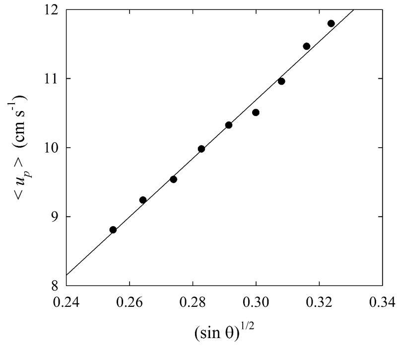
Figure J1 Plot of ensemble-averaged particle velocity 〈u〉 versus $\sqrt{\sin \mathit{\theta }}$ involving a steel sphere (R=2.5 mm) moving over glass beads (r_m=0.53 mm) giving $R/r_{\mathrm{m}}=\mathrm{4.7}$; data from Samson et al. (1998).

Because the relative smoothness $R/r_{\mathrm{m}}$ is not entirely adequate in scaling the collisional friction as c_A varies (Samson et al., 1998), it remains unclear whether these experimental conditions involve an apparent viscous-like behavior where the effective viscosity depends only on roughness geometry (Dippel et al., 1997; Samson et al., 1999) or a squared-velocity behavior as in Eq. (J7). Dippel et al. (1997) note that there is an apparent cross-over in behavior for very large and heavy spheres. Effects of the covariance of β_x and u in relation to roughness geometry and the details of motions, including transverse motions, likely are important. Nonetheless, we emphasize that in the formulations of Riguidel et al. (1994) and Samson et al. (1998), a Coulomb friction behavior is not involved.

Returning to Eq. (J1), similarly there is no clear reason to include a Coulomb-like friction term, as natural irregular particles mostly do not slide down natural rough surfaces. In addition, if the starting point involves the derivative term on the left side and the gravitational term on the right side as written, then the collisional term on the right side should be a random quantity, thus leading to a stochastic differential equation – that is, a Langevin-like equation (Riguidel et al., 1994) – not an ordinary differential equation. Moreover, the idea of a dynamic friction coefficient is misapplied in the situation where rarefied particles tumble, roll and skitter over the surface. A Coulomb model is appropriate for sustained contact, and even then a dynamic friction involves collisional friction at the surface asperity scale. Particle–surface contacts on natural granular surfaces are not smooth at a scale commensurate with a sliding Coulomb model. A rolling coefficient of friction works for spheres moving over a relatively smooth surface, not for irregular tumbling particles involving non-collinear impacts. Moreover, the static normal weight of a particle, mgcos θ, does not set the particle–surface friction. Rather, dynamic forces during collision impulses matter (Brach, 1991; Stronge, 2000). This includes the dynamic Coulomb friction force associated with conversion of translational to rotational kinetic energy during collisions (Appendix E). Any resulting dynamic friction coefficient represents an ensemble-averaged ratio of tangential to normal momentum exchanges, both of which are random variables. (This point currently is being examined in studies of bed load and eolian transport; see for example Pähtz and Durán (2018).) Finally, the experiments of Quartier et al. (2000) involved rolling a cylinder over an inclined row of cylinders in an experiment designed to remove the transverse degree of freedom of motion. The Coulomb-like term in their formulation (see their Eq. 5) arises from trapping of the rolling cylinder between bumps and is unrelated to sliding as in a conventional Coulomb model. The condition of a constant roller velocity involving an “equilibrium between gravity driving and dissipation by the shocks” is roughly analogous to isothermal conditions described in the main text, but without effects of deposition. The dynamical angle in these experiments coincides with the situation in which the velocity of the roller is sufficient to prevent trapping, “assuming a permanent contact between the roller and the rough plane”.