Assessing the effect of topography on Cs-137 concentrations within forested soils due to the Fukushima Daiichi Nuclear Power Plant accident, Japan

Topographic effects on Cs-137 concentrations in a forested area were quantitatively examined using 58 soil core samples collected in a village in Fukushima, Japan, which was directly impacted by the radioactive plume emitted during the 2011 Fukushima Daiichi Nuclear Power Plant (FDNPP) accident. In this study, five topographic parameters and two soil properties were evaluated as controls on the soil Cs-137 concentration using generalized additive models (GAMs), a flexible statistical method for evaluating the functional dependencies of multiple parameters. GAMs employing soil dry bulk density, mass water content, and elevation explained 54 % of the observed concentrations of Cs-137 within this landscape, whereas GAMs employing elevation, slope, and upslope distance explained 47 % of the observed concentrations, which provide strong evidence of topographic effects on Cs-137 concentrations in soils. The model fit analysis confirmed that the topographic effects are strongest when multiple topographic parameters and soil properties are included. The ability of each topographic feature to predict Cs-137 concentrations was influenced by the resolution of the digital elevation models. The movement of Cs-137 into the subsurface in this area near Fukushima was faster in comparison to regions affected by the Chernobyl Nuclear Power Plant accident. These results suggest that the effects of topographic parameters should be considered carefully in the use of anthropogenic radionuclides as environmental tracers and in the assessment of current and future environmental risks due to nuclear power plant accidents.

1 Introduction

On 11 March 2011, a 9.0 magnitude earthquake occurred near the northeast coast of Honshu, the largest island of Japan. A tsunami formed, arriving at the Fukushima Daiichi Nuclear Power Plant (FDNPP) approximately 1 h later. A subsequent power outage caused the water circulation pumps to fail. This then led to overheating of the water, meltdowns, and hydrogen explosions (IAEA, 2015; Mahaffey, 2014). Nearby towns, villages, and farmlands were contaminated by the atmospheric fallout from the radioactive plume. Because human and environmental exposure to levels of elevated radiation can cause adverse health effects (EPA, 2017; Wrixon et al., 2004), the Japanese government designated an area within a 20 km radius of the FDNPP to be evacuated the next day.

Table 1 Soil sampling projects conducted in the Fukushima region following the 2011 FDNPP accident (through 2019). NA stands for not available.

One of the radionuclides released to the atmosphere during the accident was cesium-137 (Cs-137). Cs-137 is an isotope of ₅₅Cs, which emits gamma rays with a half-life of 30.17 years (US EPA, 2017). Because of its long half-life, Cs-137 concentration in the environment is still a concern in Japan. Many studies have been conducted in the Fukushima region since the accident to assess the radioactivity of the land surface and environs (Table 1). Those studies confirmed that the majority of FDNPP-derived Cs-137 was concentrated in the soils close to the ground surface and exponentially decreased with depth, and that Cs-137's subsurface migration speed varied according to land use, soil types, and soil chemistry. Few studies, however, examined how local topography would affect Cs-137 concentrations accumulated by atmospheric fallout or subsequent remobilization on the land surface.

While Cs-137 is a byproduct of the nuclear energy generation process and does not exist in the environment naturally (Amaral et al., 1998; IAEA, 2015; Tsoulfanidis, 2012), it has been used since the 1960s as an environmental tracer to understand surface soil and sediment movement (Walling and He, 1997). There are two primary pathways for Cs-137 once it is released in the environment. Cs-137 lacks a single valence electron and it is positively charged, which enables it to form electrovalent bonds with organic matter and mineral anions. Once Cs-137 is deposited on the ground, it becomes adsorbed by clay minerals (Claverie et al., 2019; Fan et al., 2014; Murota et al., 2016; Nagao, 2016; Nakao et al., 2008; Ohnuki and Kozai, 2013; Park et al., 2019; Ritchie and Ritchie, 1995). It is this adsorption process that makes Cs-137 an effective environmental tracer for modeling surface soil loss, reservoir sedimentation, and sediment yield (Bennett et al., 2005; Loughran et al., 1987; Lowrance et al., 1988; Mabit et al., 2007; Martz and De Jong, 1987; Pennock et al., 1995; Quine et al., 1997; Ritchie and Ritchie, 1995; Wallbrink et al., 2002; Walling et al., 2007; Xinbao et al., 1990). Water also provides an environmental pathway for Cs-137 transport; Cs-137 has a high water solubility and it can attach to sediment within surface waters (Iwagami et al., 2015; Osawa et al., 2018; Sakuma et al., 2018; Tsuji et al., 2016).

Topographic indices such as elevation and slope should play an important role in determining Cs-137 movement in the environment because these indices affect sediment transport and hydrologic processes (Catani et al., 2010; Chen et al., 1997; Griffiths et al., 2009; Hoover and Hursh, 1943; Roering et al., 1999, 2001; Roering, 2008; Rossi et al., 2014; Yang et al., 1998). For example, Zaslavsky and Sinai (1981) noted that surface concavity was the controlling factor in distributing soil water in a catchment. Heimsath et al. (1999) examined the relationships among cosmogenic nuclides, topographic curvature, and soil depth, and concluded that the variable thickness of soil is a function of topographic curvature. Studies using Cs-137 as a tracer found that topography affects runoff and infiltration and, hence, the concentration of Cs-137 in soils (Komissarov and Ogura, 2017; Martin-Garin et al., 2012; Ritchie and McHenry, 1990; Walling et al., 1995).

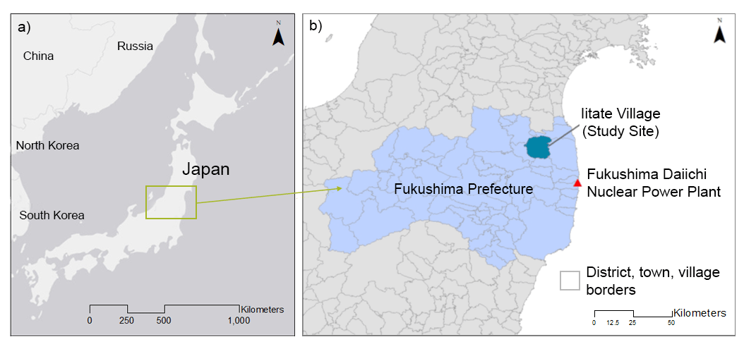
Figure 1 Locations of the FDNPP and the study site (Basemaps: a ESRI, HERE, Garmin, © OpenStreetMap contributors, and the GIS community; b ESRI Japan).

Table 2 A comparison of climates, topographies, and soil formations between the FDNPP accident-affected area and the CNPP accident-affected area.

Cs-137 accumulation patterns in the Fukushima region can be compared to the eastern European region affected by the Chernobyl Nuclear Power Plant (CNPP) accident in 1986. The CNPP and the FDNPP accidents are the only nuclear power plant accidents categorized as Level 7, which is the highest level on the International Nuclear and Radiological Event Scale (INES; IAEA, 2015; IAEA and INES, 2013; Mahaffey, 2014). The climate and topography of the Fukushima and Chernobyl regions differ (Table 2), and researchers suspect that Cs-137 concentrations on the landscape reflect these differences.

The overall goal of the research presented here is to understand the role of topography in determining the concentrations and distributions of Cs-137 on a landscape affected by the FDNPP accident. The objectives of the current study are as follows: (1) to define the concentrations and distributions of Cs-137 in surface and near-surface soil samples in a forested landscape directly impacted by the FDNPP accident and (2) to quantitatively assess the control of topographic indices and soil properties on Cs-137 concentrations in this forested landscape using predictive analytics. It is envisioned that the primary data collected will contribute toward advancing the knowledge and understanding of the environmental hazards associated with radioactive fallout, societal response, and remediation actions, as well as elucidate the movement and long-term persistence of radionuclides in terrestrial environments.

2 Methods

2.1 Study site topography and forests

Soil samples were collected in Iitate village, a forested region located 35 km northwest of the FDNPP (Fig. 1). The study site was under the plume released on 15 March 2011. The plume initially moved toward the southwest and then, following a change in wind direction, toward the northwest, resulting in wet deposition across northwestern Fukushima and other prefectures (IAEA, 2015; Fig. 2). The Fukushima region is underlain by Paleozoic metamorphic rocks and Paleozoic–Mesozoic igneous rocks (Forest Management Center, 2017). The topography is composed of mountains dissected by narrow streams and covered by deciduous and conifer trees with abundant litter on the forest floor.

Figure 2 Timing and locations of the main Cs-137 deposition events following the explosions at the FDNPP (Map: IAEA, 2015).

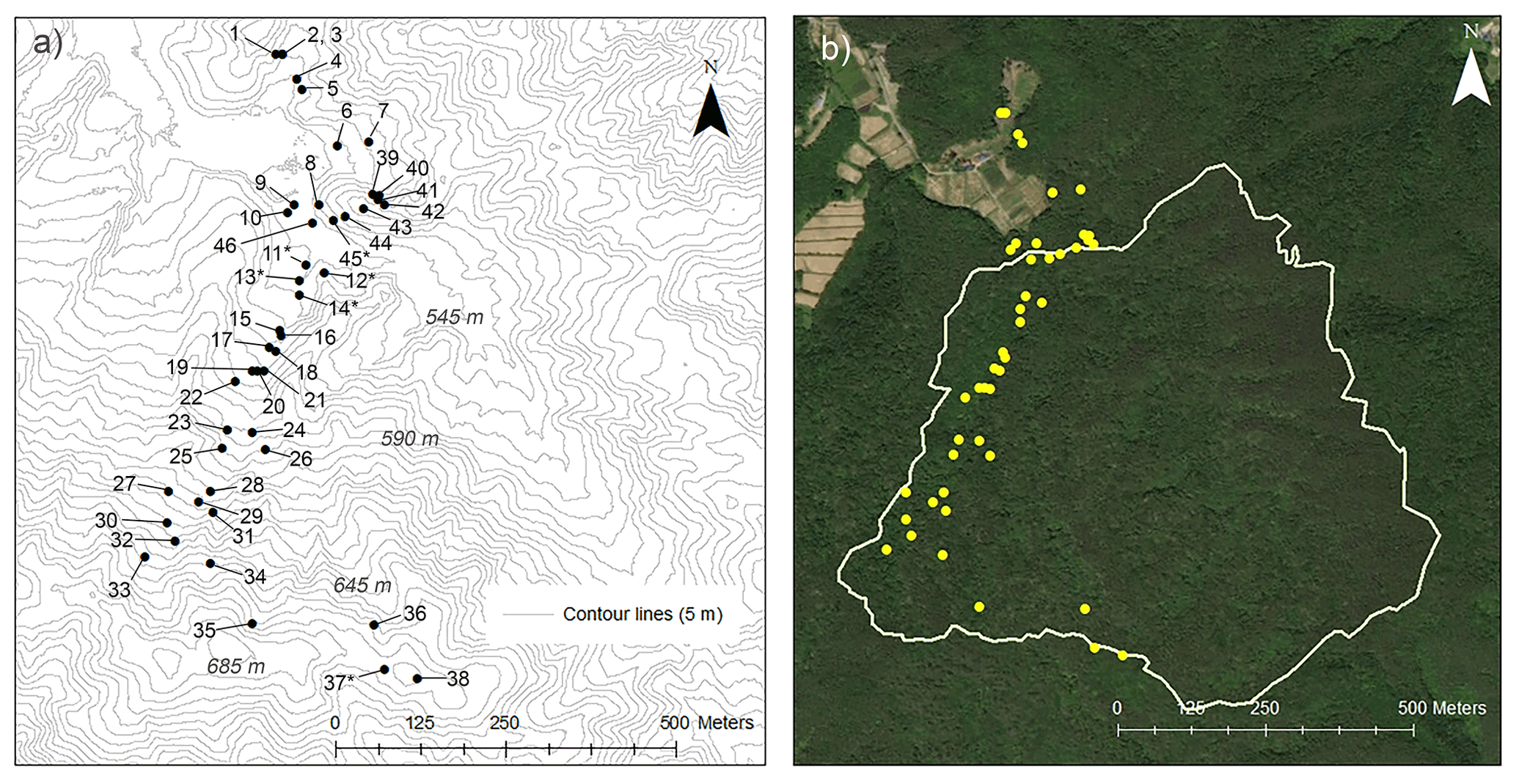
Figure 3 Study site topography and aerial images. (a) Numbered sample locations where multi-year samples were collected at the locations marked by ^* and contour lines are at 5 m intervals (Basemap: ESRI). (b) A large basin enclosing the longest slope (Basemap: ESRI).

The topography and sampling locations are shown in Fig. 3. The maximum change in elevation of the sampling points is 135 m, and the largest basin area in the study site is 0.56 km². From late spring to autumn, the trees form a canopy over the hills, and the visibility of the sky from the ground is limited. On the south edge of the largest basin, the forest canopies are thin, and the nearby hills toward the southeast, in the direction of the FDNPP, are visible.

Some parts of the forests in the study site are not native. Overall, 31 % of Fukushima forests are planted (Fukushima Prefecture, 2021). Because no major forestry work had been conducted in the area after the accident, land use history was not considered in the analysis.

2.2 Soil sample collection

Soil samples were collected during the summer in 2016, 2017, and 2018. In 2016, samples were collected at locations 1 to 20, 44, and 45 (Fig. 3a) to cover accessible hillslope areas from the lowlands in a circular pattern. The 2017 sampling campaign sought to confirm anomalies observed in previous year and to check the Cs-137 concentration at the highest elevation by collecting samples at locations 11 to 14, 38, and 46. In 2018, the sampling activity focused on the southwest slope and the eastern side by collecting samples at 11 to 14, 21 to 37, 39 to 43, 45, and 46. Most sampling locations were on the southwest slope due to accessibility. In sum, there were 46 total sampling locations, multiple-year samples were collected at eight locations (averaged herein), and the total number of samples collected was 58. Coordinates were recorded at all sampling locations.

For sample collection, a sampler 5 cm in diameter and 30 cm long from Daiki Rika Kogyo Co., Ltd., Japan, was used. The circular tube was made of metal and contained a replaceable plastic liner. The sampler was tamped into the ground with a hammer. Once fully inserted, the sample was pulled out, and the plastic liner containing the soil was removed, sealed, and taken to the University of Tokyo.

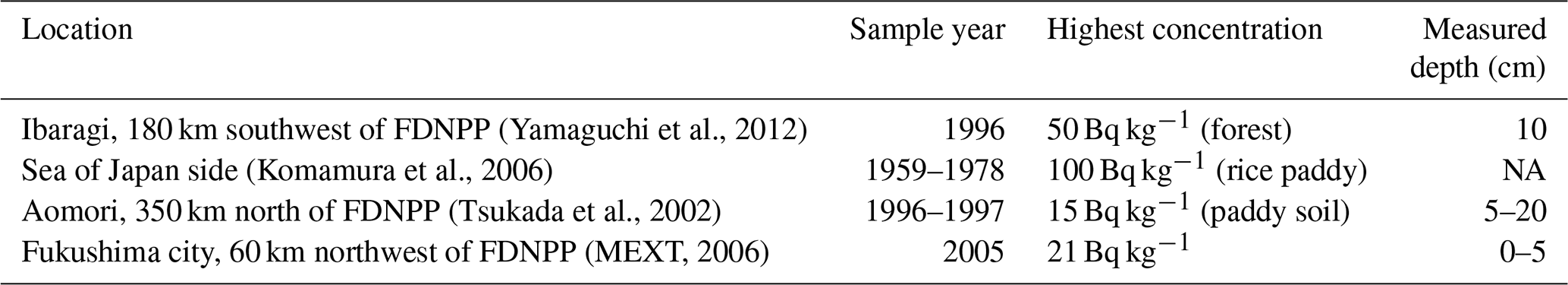
Table 3 Background levels of Cs-137 in soils in Japan before the FDNPP accident (the highest concentration at a measured soil depth). NA stands for not available.

2.3 Soil property and radioactivity measurements

In the laboratory, each plastic tube was opened, photographed, divided into 2 cm thick disks from the surface to a depth of 20 cm, and 2.5 cm thick disks from depths of 20–30 cm. All visible plant roots or rocks were removed. Each disk sample was placed on a plate, weighed, and dried in an oven for 24 h at 105 ^∘C. The drying time was extended as necessary to achieve consistent dryness across the samples. The dried sample was reweighed, placed in a mortar, disaggregated, and particles larger than 2 mm were removed. Mass water content (%) and soil dry bulk density (g cm⁻³) were calculated for each disk sample. Textural analysis (sand, silt, and clay) was performed on approximately one-half of all soil samples using the pipette method. The samples were selected so that various soil types, colors, locations, and elevations were represented. Organic matter in the soil samples was broken up by placing the sample into a beaker, adding hydrogen peroxide (H₂O₂), and placing the beaker into a 100 ^∘C water bath for 4–5 h. The next day, sodium hexametaphosphate ((NaPO₃)₆) was added to the samples, which were shaken with a sonic homogenizer. As soon as the sample was placed onto the desk, suspended sediment was collected using a pipette at 20 s for sand (≥0.05 mm) and 4 h for clay (<0.002 mm) to determine the texture class of the sample. Each fraction was dried in the oven and weighed, and its fractional percentage determined. Silt fraction percentage was calculated from the results at 20 s and 4 h. To verify the percentage of clay, selected samples were tested using SALD-7500nano (nano-particle size analyzer, Shimadzu Corporation, Kyoto, Japan).

Processed samples were stored in polyethylene vials and sent to the Isotope Facility for Agricultural Education and Research, University of Tokyo, for analysis. Radioactivity levels were measured with a NaI(Tl) scintillation automatic gamma counter (2480 WIZARD2 gamma counter, PerkinElmer Inc., Waltham, MA, USA), which was equipped with a well-type NaI(Tl) crystal 7.6 cm in diameter and 7.6 cm long, and covered with a 75 mm thick lead shield. Energy calibrations were performed using the 662 keV (kiloelectron volts) energy peak of gamma rays from Cs-137. For radiocesium, the detection limit was approximately 0.5 Bq. After each measurement, the radiation was separated into radiation emitted by Cs-137 and Cs-134 using the abundance ratio of Cs-137 to Cs-134 at the time of sampling. This ratio was obtained from the physical decay rates of the isotopes and the elapsed time from the accident to sampling, assuming that the ratio at the time of the FDNPP accident was 1:1 (Nobori et al., 2013; Tanoi et al., 2019). Although a gamma-ray spectrometer provides more precise Cs-137 measurement data, lower-resolution NaI with effective algorithms can be accurate, and it is preferred for its ruggedness, shorter time required for evaluation, and cost of operation (Burr and Hamada, 2009; Stinnett and Sullivan, 2013). The US Environmental Protection Agency allows the NaI method for gamma-ray measurement (EPA, 2012).

In this study, Cs-137 values are reported in two units: Bq kg⁻¹ or Cs-137 activity measurement per volume, and Bq m⁻² or mass depth (Bq kg⁻¹ × soil dry bulk density × sample thickness). Since soil bulk density varies across samples, mass depth indicates the functionality of soil bulk density as an explanatory variable, and it provides a means to compare concentration levels among samples with varied soil bulk densities (Kato et al., 2012; Miyahara et al., 1991; Rosén et al., 1999). Cs-137 values among samples were decay normalized to 28 June 2016 (see Appendix A), which enabled a comparison of measurements conducted on different dates, and the sum total of Cs-137 in the entire tube is called “core total”.

Background Cs-137 contamination data before the FDNPP accident were unavailable for the study site. According to previous work, Cs-137 activities in Japanese soils varied from ≤15 to 100 Bq kg⁻¹ before the accident (Table 3). Although the 100 Bq kg⁻¹ measurement was an outlier, this value was used as the conservative background contamination level in the following analysis.

2.4 Digital elevation models

This study employed two digital elevation models (DEMs). The 1 m resolution DEM was provided by the Forestry and Forest Products Research Institute, Japan. Its original datum was GCS JGD 2011 (Zone 9), and the data collection year was 2012. The 10 m resolution DEM was downloaded from the Geospatial Information Authority of Japan (https://www.gsi.go.jp/kiban/, last access: 13 January 2018) website. Its file date was 1 October 2016, and the original datum was GCS JGD 2000. The coordinate projection of all GIS files, including DEMs, was set to UTM 54N (WGS 1984).

Analysis of geomorphic processes can be affected by spatial resolution (Claessens et al., 2005; Martinez et al., 2010; Miller et al., 2015; Sørensen and Seibert, 2007). Using multiple DEMs enables researchers to identify resolution dependency of specific topographic features (Gallant and Wilson, 1996; Kim and Lee, 2004; Moore et al., 1993).

The topographic parameters for analysis were selected based on the following assumptions.

• Elevation: soil particles with adsorbed Cs-137 move down a sloped surface, suggesting that Cs-137 concentration in surface soils would be higher at lower elevations (Martin, 2000; Roering et al., 1999).

• Slope: slope influences the downward mass movement on a surface (Roering et al., 1999).

• Upslope distance to the basin edge: assuming Cs-137 continuously moves down a sloped surface, the longer the upslope distance, the higher the Cs-137 concentrations (Komissarov and Ogura, 2017; Roering et al., 1999, 2001).

• Surface plan curvature and topographic wetness index (TWI): Cs-137 moves into the subsurface by infiltration (Schimmack et al., 1989, 1994; Teramage et al., 2014). Cs-137 concentrations would be higher where water ponds, and Cs-137 would migrate to a greater depth in the same temporal period, compared with other locations where water does not pond. Slope profile and surface plan curvature are influential factors in hydrology and soil transport on a sloped surface; hence, they would influence Cs-137 accumulation (Gessler et al., 1995; Heimsath et al., 1997; Momm et al., 2012; Moore et al., 1993; Tesfa et al., 2009). The topographic wetness index (TWI) is frequently used in surface hydrology assessments (Hengl and Reuter, 2008). This index reflects water's tendency to accumulate at any point in a catchment (Quinn et al., 1991), and it is calculated as the natural log of total upslope area divided by the tangent of hillslope gradient (Quinn et al., 1991, 1995).

The elevation of sampling locations was extracted from the DEMs using the raster extract function in the R package (R Core Team, 2015). SAGA GIS (Conrad et al., 2015) was used to compute slope and plan curvature because this function has multiple options for the curvature calculation setting. The method used for plan curvature calculation was the second-order polynomial based on the elevation values in nine surrounding cells (Zevenbergen and Thorne, 1987). The “D-Infinity Distance Up” tool of TauDEM was used to compute the upslope distance (Tarboton, 1997), which calculates the distance from each grid cell up to the ridge cells according to the reverse flow path directions. Here, the “minimum” distance and “surface” (total surface flow path) distance calculation options were used. TauDEM also was used to calculate TWI values. All topographic calculations in SAGA and TauDEM were saved as .tif files. The “raster::extract” function of the R package was used to extract each topographic value for sampling locations.

2.5 Generalized additive models

The sampling locations were influenced by terrain access, so they were not randomly selected or uniform, and the number of samples was small compared with the sampling area size. Thus, distance-based spatial analyses such as semivariograms would not be appropriate, and a regression approach was adopted.

Multiple regression methods (linear, polynomial, logarithm, and bi-splines) were run to check the relationships between Cs-137 measurements and the topographic parameters and the soil properties. The resulting regression plots showed fitting curves with multiple knots, and most of the topographic parameters had non-linear, complex relationships with Cs-137 accumulation patterns. Thus, generalized additive models (GAMs) were employed. GAM replaces the linear predictor of a linear additive model with a sum of smooth functions of predictor variables (non-parametric) (Hastie and Tibshirani, 1990; Wood, 2017; Wood et al., 2016). The smoothing parameter of GAM controls the trade-off between the smoothness of the fit and the closeness of the fit to the data (Wood, 2017; Eq. 1).

$$\begin{array}{}\text{(1)}& g\left({\mathit{\mu }}_i\right)=A_i\mathit{\theta }+f_{\mathrm{1}}\left(x_{\mathrm{1}i}\right)+f_{\mathrm{2}}\left(x_{\mathrm{2}i}\right)+f_{\mathrm{3}}\left(x_{\mathrm{3}i}\right)+\mathrm{\dots }{f}_k\left(x_{ki}\right),\end{array}$$

where x₁, x₂, …, x_k are explanatory variables (predictors), μ_i≡E(expected)(Y_i) and $Y_i\sim \mathrm{EF}({\mathit{\mu }}_i,\mathit{\varphi })Y_i$ are response variables, EF(μ_i,ϕ) denotes an exponential family distribution with mean μ_i and a scale parameter ϕ, A_i is a row of the model matrix (parametric), and θ is a corresponding parameter vector. Finally, f_j are smooth functions (non-parametric) of the covariates, x_k. In GAM algorithms, models are estimated by minimizing squared errors with an increasing penalty as the curves become less smooth.

GAMs allow flexible specification of the response variable dependence on predictors according to the smooth function rather than parametric relationships (Wood, 2017). Because a smooth function is estimated for each covariate, when multiple predictors are included in a model, it is a sum of these functions and a constant.

GAM users can examine the significance and the model fit of each predictor and the overall model performance with multiple indicators (model knots, effective degree of freedom, F statistic, p value, R², and deviance-explained percentage). Deviance-explained percentage is the proportion of the total deviance explained by the model. This serves as a generalization of R² in GAM. While overfitting can be a potential problem of GAM (Friedman and Stuetzle, 1981), GAMs work well when users aim to detect the significance of predictors, and the baseline relationship between the predictors and the response variable in a complex model environment (Hastie and Tibshirani, 1990; Linnik et al., 2020; Tesfa et al., 2009).

3 Results

All primary data collected in the field campaign, processed in the laboratory, and derived from the DEMs are summarized in Appendix B.

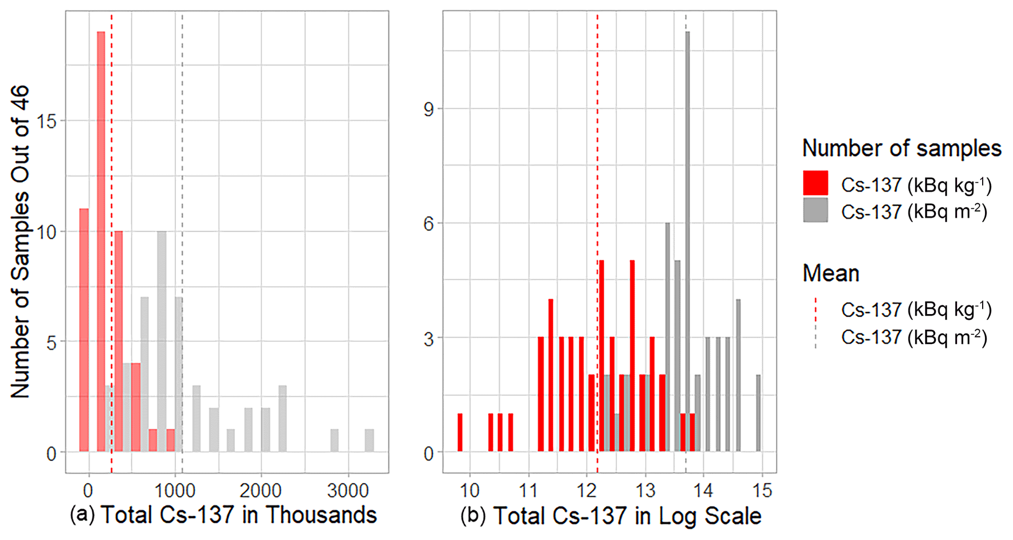
Figure 4 Distribution of mass-based total Cs-137 in a core sample. (a) A unit of each bin is 200 k. (b) Distribution of total mass depth Cs-137 in a core sample in a log scale (red: Cs-137 kBq kg⁻¹; gray: Cs-137 kBq m⁻²).

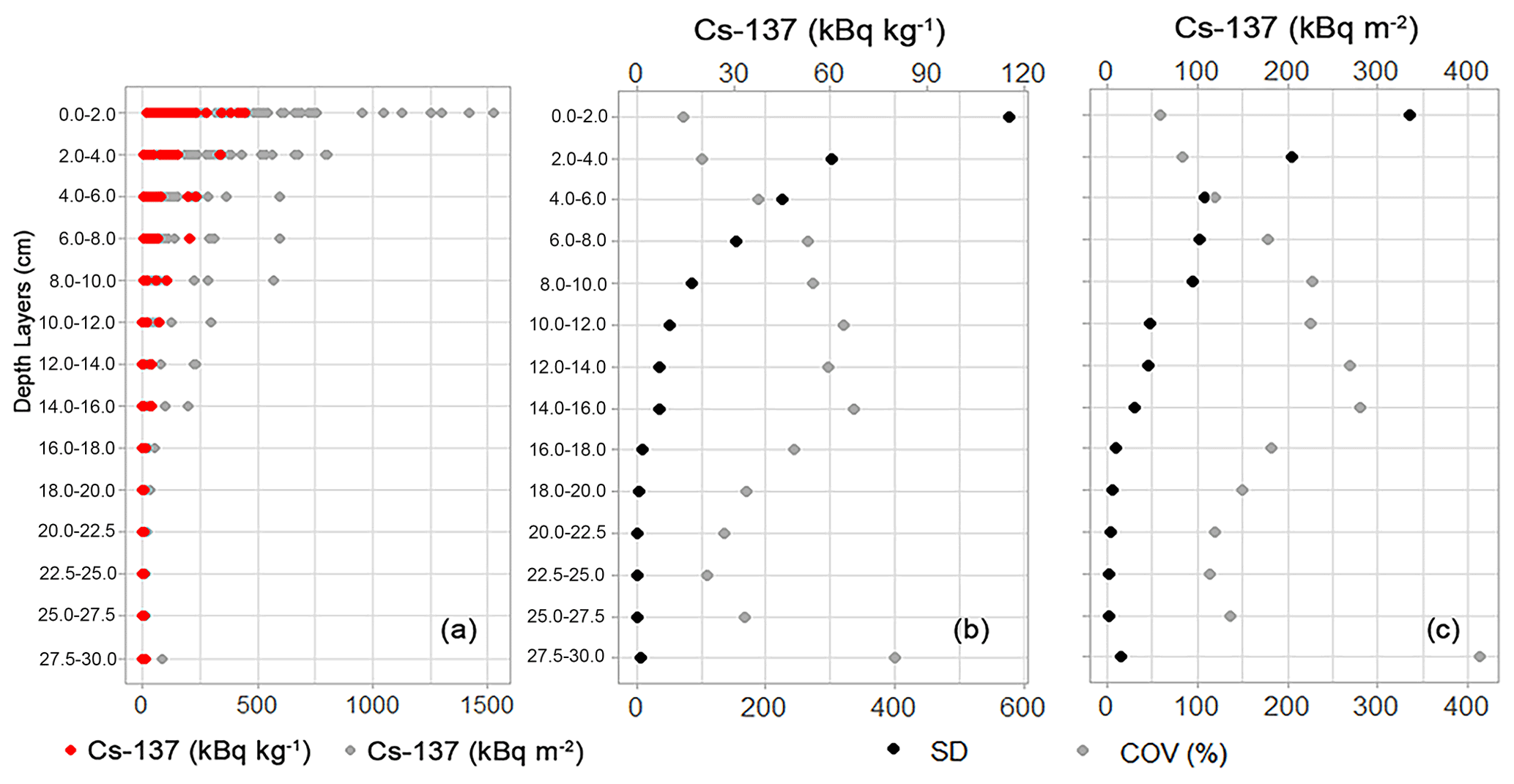
Figure 5 (a) Depth distributions of Cs-137 concentrations in kBq kg⁻¹ (red) and kBq m⁻² (gray). Standard deviations (red) and COVs (gray) by depths in (b) kBq kg⁻¹ and (c) kBq m⁻².

3.1 Cs-137 concentration distributions among core samples

Figure 4a shows the binned distributions of core total Cs-137 values in kBq kg⁻¹ (red) and kBq m⁻² (gray), as well as their means (Fig. 4b in a log scale). When measured in kBq kg⁻¹, the Cs-137 values clustered in six bins, and 41 % of the core samples were in the 100–300 kBq kg⁻¹ interval (Fig. 4a: red). When measured in kBq m⁻², Cs-137 values spread across 13 bins (Fig. 4a: gray). The average total core Cs-137 values among these samples were 267 kBq kg⁻¹ and 1075 kBq m⁻².

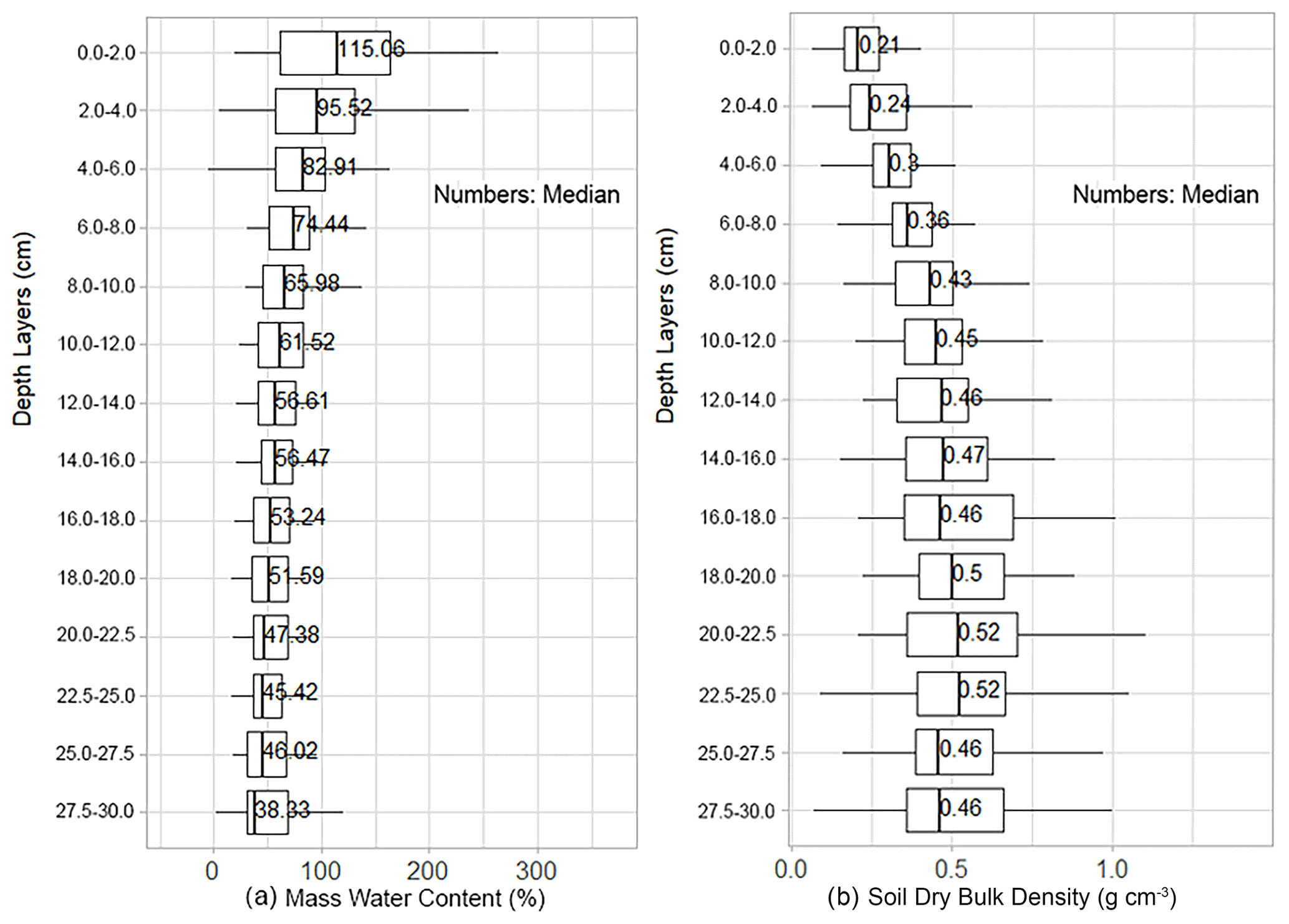
Figure 6 Depth profiles of (a) mass water content (%) and (b) soil dry bulk density (g cm⁻³).

Cs-137 activities exponentially decreased with depth in both kBq kg⁻¹ and kBq m⁻² (Fig. 5a). These vertical profiles are similar to the results reported in previous studies (Fujii et al., 2014; Koarashi et al., 2012; Matsunaga et al., 2013; Takahashi et al., 2015; Tanaka et al., 2012; Teramage et al., 2014). The current samples were collected 5–7 years after the FDNPP accident, and the soils still held the largest amount of Cs-137 in the uppermost layer. The average depth of 90 % concentration (90 % of the entire Cs-137 in a core sample) was 6.1 cm in kBq kg⁻¹ and 6.9 cm in kBq m⁻². Standard deviations of Cs-137 activities were up to 115 kBq kg⁻¹ and 335 kBq m⁻² in the upper 2 cm depth (black dots in Fig. 5b and c). The relative variability among samples (coefficient of variations; COVs) was below 100 % in the top layer, and COVs increased toward the 14–16 cm depths and decreased again for both units (gray dots in Fig. 5b and c).

3.2 Soil properties

Figure 6 displays the averages of mass water content (%) and soil dry bulk density (g cm⁻³) for each depth layer. Gravel (below the mid-depth from two disks) and visible roots (at the ground surface from several samples) were removed, which decreased the dry bulk densities of select samples.

Soil texture affects the amount of adsorbed Cs-137 per unit mass of soil particles and accumulation patterns of Cs-137 in soils (Bennett et al., 2005; Giannakopoulou et al., 2007; Korobova et al., 2016; Walling and Quine, 1992). On average, the tested soils contained >50 % sand, and most of the samples were in the categories of sand, loamy sand, sandy loam, and loam (Appendix B).

The average mass water content percentage at the ground surface was above 100 % (Fig. 6a). The standard deviations of water content in the uppermost soil layers were >50 % and the deviation percentages decreased with depth. Some samples collected near the surface exceeded field capacity, likely due to poor drainage, soil texture, and/or high organic content.

Soil dry bulk density and its standard deviation increased with depth (Fig. 6b). The average dry bulk density of all disk samples was 0.45 g cm⁻³, and the densities ranged from 0.06 to 1.43 g cm⁻³. The Japanese agricultural soil profile physical properties database, Solphy-J, compiled data for 1800 categories of Japanese soils (Eguchi et al., 2011). This database shows that the soil dry bulk densities of Japanese orchard soils range from 0.80–1.44 g cm⁻³. Fujii et al. (2014) collected soil samples to 20 cm depth at five locations in Fukushima forests, and these soil dry bulk densities ranged from 0.3–0.7 g cm⁻³. The relatively low bulk density in this study agrees well with previous work.

3.3 Cs-137 concentration distribution on representative slope

Figures 7 and 8 organize the core total Cs-137 concentration of all samples by elevation and slope extracted with the 10 m DEM. Migration head depths have been added to Fig. 7, defined as the depth at which Cs-137 activity (Bq kg⁻¹) decreased to the conservative background activity level (i.e., 100 Bq kg⁻¹). This study considers the head depth as the deepest subsurface migration point of the FDNPP-derived Cs-137. These figures provide an overview of Cs-137 distribution patterns on the hillslopes. Numbers 1–4 are added to the graphs to indicate the highest concentration samples in Bq m⁻². The elevation data were extracted from the 10 m resolution DEM.

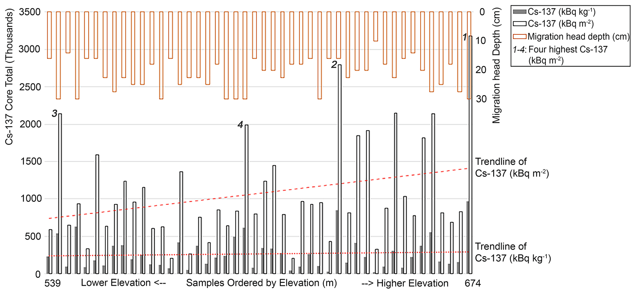
Figure 7 Core total Cs-137 in both units along the elevation (m). Numbers 1–4 indicate the samples with the four highest Cs-137 concentrations in kBq m⁻². Migration head depths (cm) are the depths at which Cs-137 concentrations decreased to 100 Bq kg⁻¹ in a core sample.

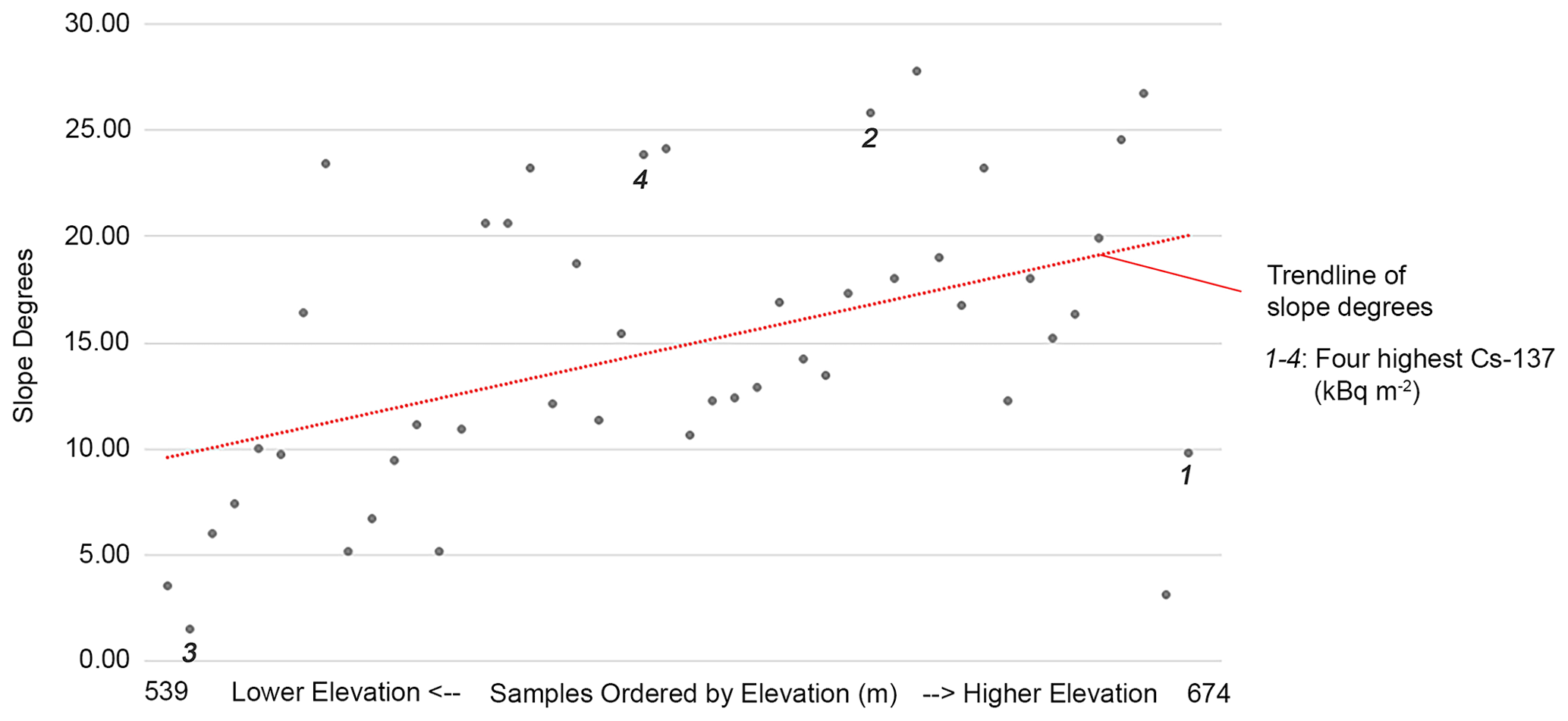
Figure 8 Slope (degrees) of sampling points along the elevation (m). The numbers 1–4 correspond to the same numbers in Fig. 7.

Cs-137 activities in kBq m⁻² units increase with elevation (p value is 0.03), but this trend was not observed for Cs-137 concentrations in kBq kg⁻¹ (Fig. 7). The migration head depths of three of the samples with the highest Cs-137 concentrations had reached the end of the sampler (30 cm), and the average migration depth among all samples was 21.7 cm. Two of the four highest Cs-137 concentrations were at the highest elevation and near the bottom of a hill (Fig. 7), and they were locations with relatively low slopes (Fig. 8). The remaining two samples with the highest Cs-137 concentrations were at 24–26^∘ slopes, which are two of the steepest sampling locations. Elevation and slope do not appear to explain the distribution of Cs-137 concentration, suggesting that additional topographic parameters may be required.

3.4 GAM assessment

Model assessment will focus on eight parameters: Cs-137, five topographic parameters, and two soil properties. This study used mgcv in the R package (Wood et al., 2016) for GAM calculations. The model setting was consistent for all model runs, except rotating predictors (see Appendix A).

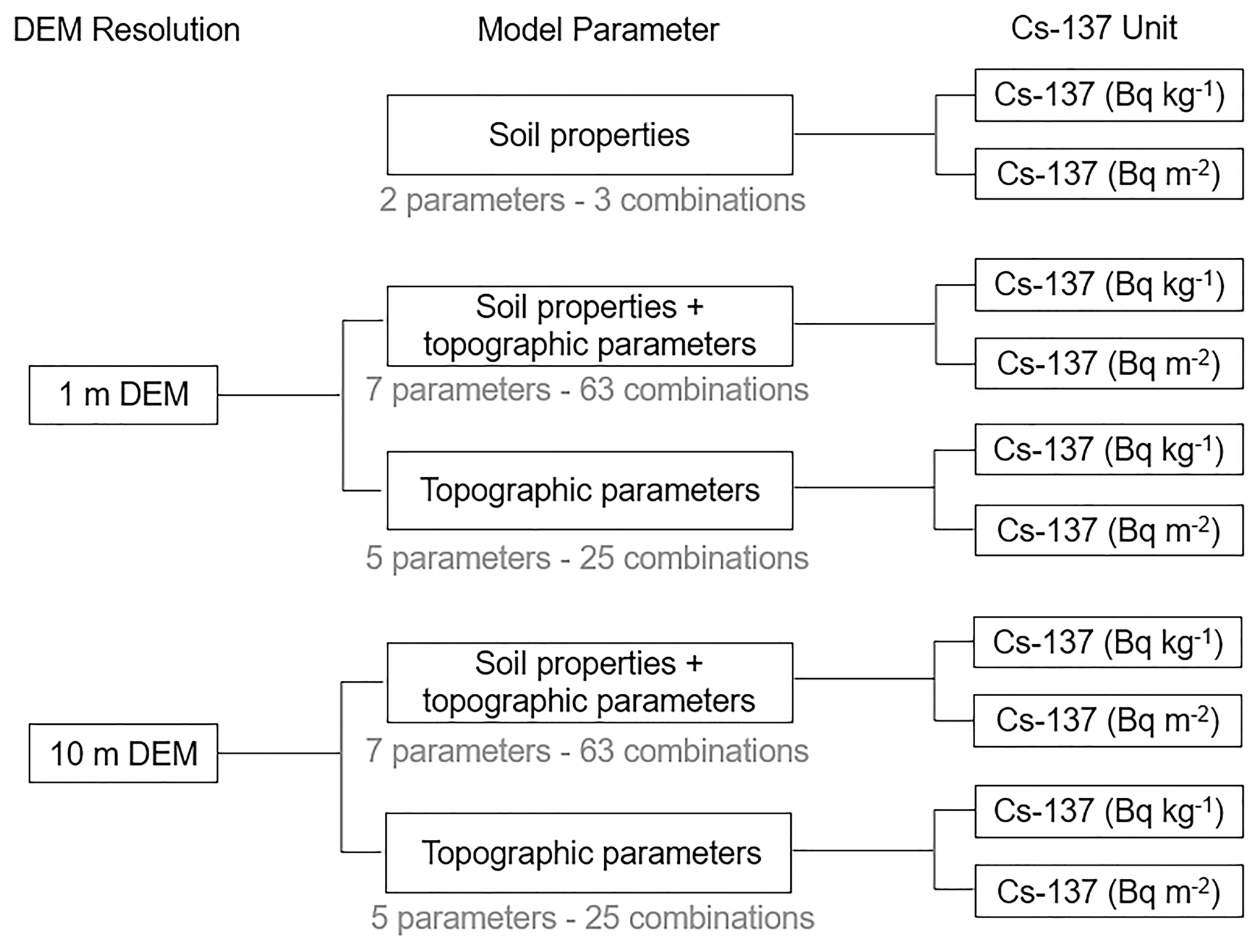
First, GAMs were run with a single topographic parameter or one of the soil properties. Then models with parameter combinations were run to assess the interactions among the parameters. Combinations with more than three parameters were not tested to avoid overfitting and to identify parameters with distinct influences on Cs-137 concentrations. The total number of possible combinations was 63 – combinations of seven parameters, including five topographic parameters (elevation, slope, upslope distance, plan curvature, and TWI), and two soil properties (water content and soil dry bulk density), not considering the parameter orders (Fig. 9). Among the 63 combinations, three were only soil properties (combinations of two properties), 25 were only topographic parameter(s) (combinations of five predictors), and the remaining 35 were mixed soil properties and topographic parameters. Then, the same GAM with topographic parameter(s) was executed four times against Cs-137: topographic parameters extracted from the (1) 1 m and (2) 10 m DEMs, and with units of (3) Bq kg⁻¹ and (4) Bq m⁻². Soil parameters are not affected by DEM resolutions (Fig. 9).

Figure 9 GAM parameter combinations.

GAMs were executed against each depth layer to check model performance as affected by changes by depth. Topographic parameters have one distinct value for an entire core sample, such as elevation and slope. Thus, when a model included a topographic parameter, the model check was a “one-to-many” relationship (topographic parameters to Cs-137 in multiple depth layers). Soil properties had a measurement for each depth layer. Thus, when a model included a soil property, the prediction was a “one-to-one” relationship (soil property in a depth layer to Cs-137 in the depth layer).

GAM accuracies were evaluated by three indicators: Akaike information criterion (AIC), generalized cross validation (GCV), and R² (see Appendix A). These model parameters were extracted from mgcv outputs in the R package. The AIC is a weighted sum of the log likelihood of the model and the number of fitted coefficients. The lower the AIC indicates a better model fit (Bivand et al., 2008). GCV is a simplified version of cross validation that checks model fit by removing one data point at a time. GCV can be used in a similar way as AIC to measure the relative performance of multiple models.

Table 4 The results of single topographic parameter GAMs for deviance-explained percentages and the number of depth layers where p values were equal to or less than 0.05. “( )” indicates standard deviation.

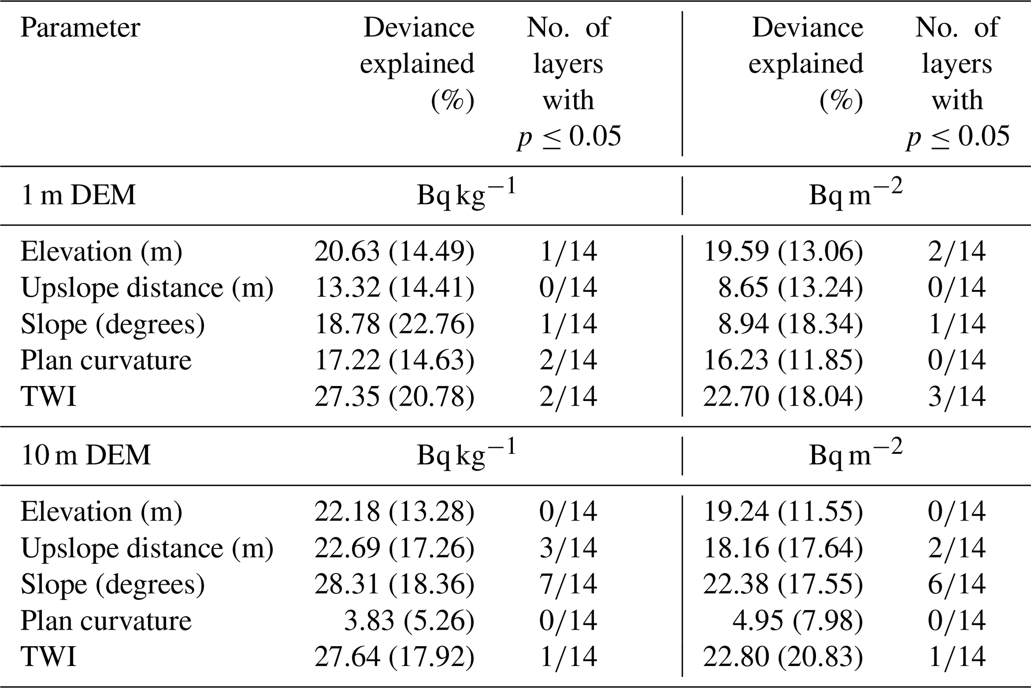
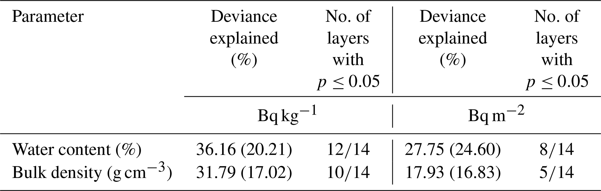
Table 5 The results of single soil property parameter GAMs for deviance explained and the number of depth layers where p values were equal to or less than 0.05. “( )” indicates standard deviation.

Identifying outliers is vital for understanding model errors and capturing influential factors not included in the model. Cook's distance method was used for outlier identification (Cook, 1977; see Appendix A). Cook's distance identifies influential data points by checking how the fitted model parameters change when an outlier data point is removed. Cook's outliers were extracted from linear regression summary plots using the R package (Stevens, 1984).

There was no reference data from other sites to validate the model prediction accuracy. Therefore, Cs-137 concentrations were reverse-predicted by applying the two best-performing prediction models to the original data. Here, mgcv's “predict.gam( )” in the R package was used to generate the predictions.

3.5 GAM performance

In Tables 4 and 5, the percentage of deviance explained shows the average values for the 30 cm depth for single-parameter model results. The p value columns show the number of depth layers in which the average p values were equal to or less than the significance threshold (p≤0.05; e.g., “$\mathrm{4}/\mathrm{14}$” means that four depth layers had p≤0.05). Table 4 includes the model results with each topographic parameter that varied with DEM resolution. Table 5 displays the model results with each soil property parameter, whose values were unaffected by the DEM resolution. None of the single-parameter models returned average deviance-explained percentages greater than 36 %, which was the model with water content. The lowest average p value was 0.05, which was also the model with water content. Among topographic parameters, TWI was the most effective predictor with the 1 m DEM (27 %), and slope was the most effective predictor with the 10 m DEM (28 %). Elevation and slope explained Cs-137 deviance better with 10 m DEM than with 1 m DEM. Topographic parameters explained Cs-137 deviance at higher percentages in Bq kg⁻¹ units than in Bq m⁻² units, except plan curvature. Soil properties explained Cs-137 deviance at higher percentages than did the topographic parameters. Like the topographic parameters, the soil properties model explained Cs-137 deviance at higher percentages in Bq kg⁻¹ units than in Bq m⁻² units.

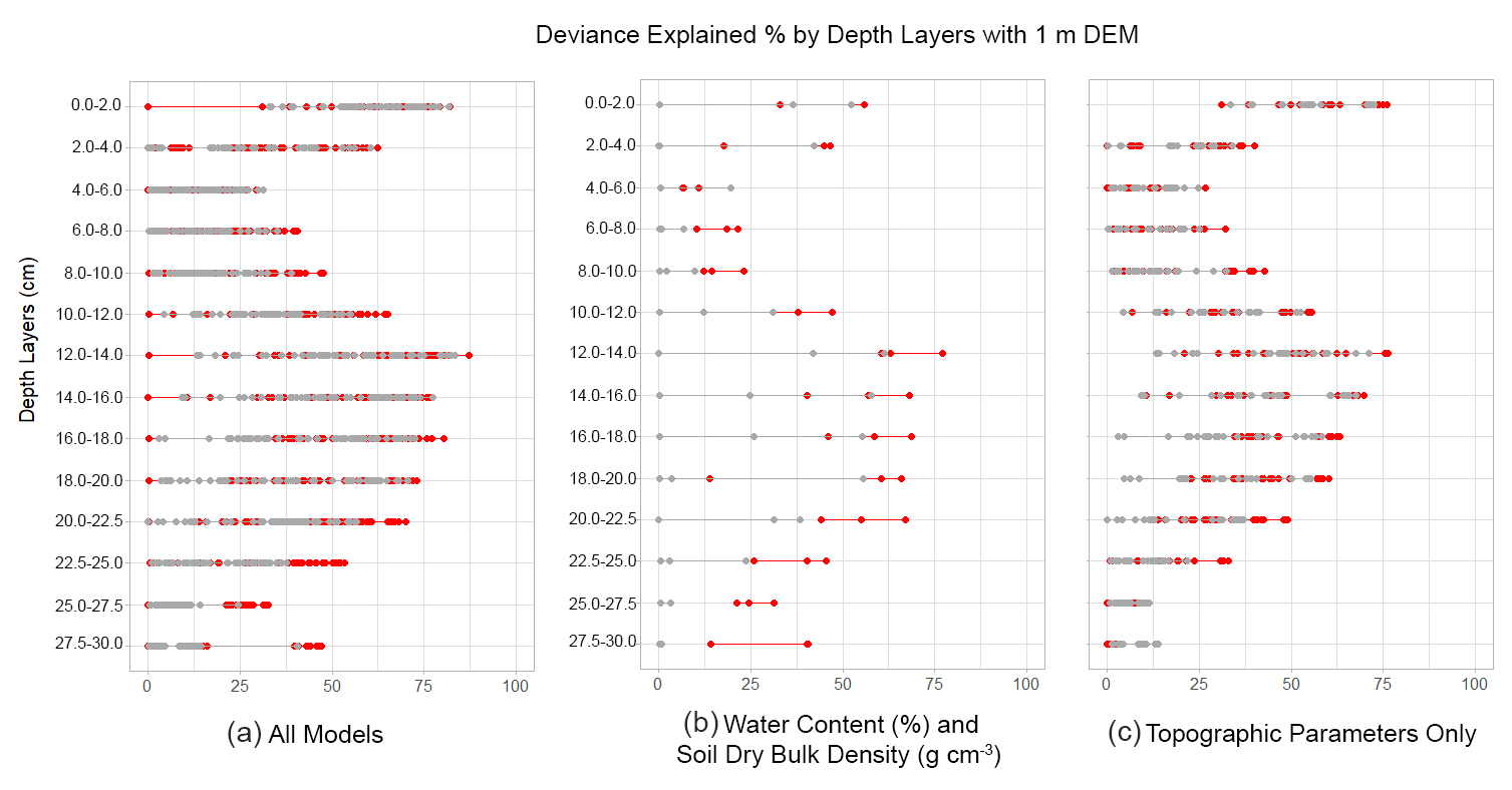
Figure 10 Deviance-explained percentages using the 1 m DEM. (a) All parameter including combinations soil properties and topographic parameters. (b) Parameter combinations with only water content (%) and soil dry bulk density (g cm⁻³). (c) Parameter combinations with only topographic parameters.

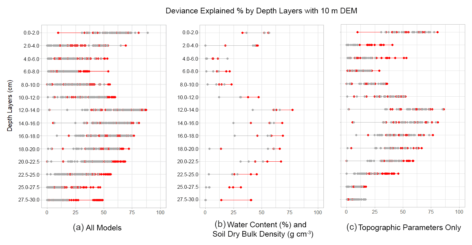
Figure 11 Deviance-explained percentages using the 10 m DEM. (a) All parameter combinations soil properties and topographic parameters. (b) Parameter combinations with only water content (%) and soil dry bulk density (g cm⁻³; the same graphic in Fig. 10 is repeated for the comparison purpose). (c) Parameter combinations with only topographic parameters.

Figures 10 and 11 display the deviance-explanation percentages of GAMs with combinations of parameters, where the red and gray dots represent the deviance-explanation percentages of Cs-137 in Bq kg⁻¹ and Bq m⁻² units, respectively. The average correlation index between the average deviation explanation percentages and p values throughout the depth was −0.64. That is, higher explanation percentages returned lower p values.

Table 6 The most effective parameter combinations with the best deviance-explained percentages and the number of depth layers where p values were equal to or less than 0.05. “( )” indicates standard deviation. The two models given in bold, [A] and [B], returned the best model performance with the 10 m DEM and were used for reverse prediction accuracy checks.

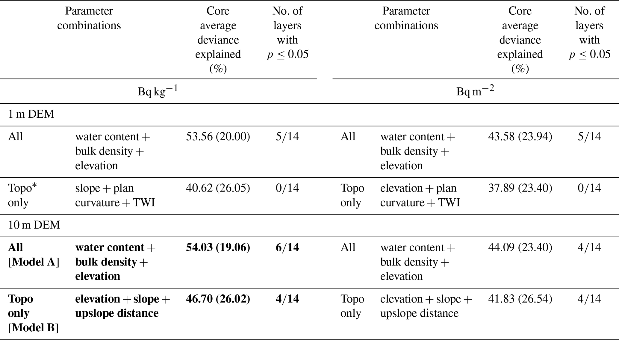
^* An abbreviation of “topography”.

The combination parameter models explained Cs-137 deviance in Bq kg⁻¹ (red dots) at higher explanation percentages on average than deviance in Bq m⁻² (gray dots) for both DEMs, and all six figures showed similar vertical S curves (Figs. 10 and 11). The deviance-explained percentages of some models were over 75 % for the top layer; the percentages explained decreased with depth, then increased again toward the 12–14 cm depth. These S-shaped curves resemble the vertical profiles of the COVs of Cs-137 measurements (Fig. 5b and c), and the curves were observable for models with only soil properties and only topographic parameters.

The most effective parameter combinations for explaining Cs-137 deviance are summarized in Table 6. The rows are separated into the model combinations with a mix of soil and topographic parameters, and the model combinations with only the topographic parameters. The most effective combinations for predicting Cs-137 deviance were “water content + bulk density + elevation” for models with both 1 m (53.56 %) and 10 m (54.03 %) DEMs. The most effective topographic parameter combinations were “slope + plan curvature + TWI” when using the 1 m DEM (40.62 %) and “elevation + slope + upslope distance” when using the 10 m DEM (46.70 %). The combination models returned higher explanation percentages using the 10 m DEM and Cs-137 in Bq kg⁻¹ units.

Two models with the highest explanation percentages in Table 6 are identified as Model A and Model B. These will be used for reverse prediction accuracy checks.

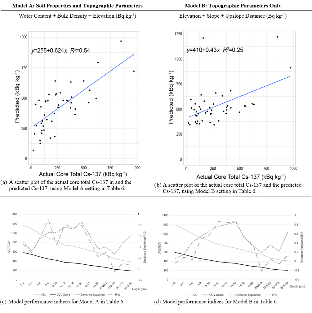
Figure 12 (a, b) Regression analysis of actual and predicted Cs-137 activities. (c, d) Model fit diagnosis results of the best-performing models (light gray: AIC; black: GCV score; dashed: deviance-explained percentage: loosely dash-dotted: R²). Higher deviance-explanation percentages and R² values indicate how well the model explained, or approximated, the real data points. Lower AIC indicates a good model with less information loss (parsimony), and lower GCV suggests a good model with a smaller prediction error (Hastie et al., 2009; Wood, 2017).

The two models in Table 6 that had the best performance were applied to the original data to reverse predict Cs-137 concentrations with the 10 m DEM, and model accuracies were checked. Regression analyses between the actual and predicted Cs-137 values returned R²=0.54 for Model A with soil properties and elevation (Fig. 12a). Model B with only the topographic parameters returned lower R²=0.25 (Fig. 12b), overestimating two data points at 400–1000 Bq kg⁻¹. With increased depth, model fit (AIC and GCV) continues to improve while the Cs-137 standard deviations decrease (Fig. 12c and d). The explanation power of the model (deviance explained and R²) was the highest at the mid-depth region, where the relative variance of Cs-137 was the largest (Fig. 5b and c).

Table 7 Comparison of Cs-137 downward migration depth between the CNPP accident-affected area and Fukushima at about the same length of time after the nuclear plant accidents. Values in the current study are not decay normalized.

Four outliers were identified on the basis of Cook's criterion. Two of the outliers (samples 37 and 38 in Fig. 3) were at the highest elevation on the basin ridges with a flat surface. The third outlier (sample 23 in Fig. 3) was at a location with a lower TWI (in the first quantile) and a 26^∘ slope. This sample did not show extreme values in Cs-137, water content, or soil dry bulk density, but the migration head depth of the sample was one of the deepest at 16 cm. The fourth outlier (sample 32 in Fig. 3) was near the basin edge and at a location with a 15^∘ slope, and concave curvature. This sample had the highest water content in the uppermost layer (0–2 cm). Outlier samples 23 and 37 in Fig. 3 had the highest Cs-137 concentrations in Bq kg⁻¹.

4 Discussion

4.1 Explanatory Power of GAM

The GAM results demonstrated about 50 % of Cs-137 deviance was explained by three parameters (Table 6). Model performance might be improved by including factors such as surface vegetation and subsurface organic matter (Claverie et al., 2019; Doerr and Münnich, 1989; Dumat et al., 1997, 2000; Fan et al., 2014; Korobova et al., 2016; Mabit et al., 2008; Staunton et al., 2002; Takenaka et al., 1998; Tatsuno et al., 2020). Topography itself did not explain the entire Cs-137 concentration patterns in the forest; however, the influence of topography on Cs-137 concentration patterns was measurable.

Elevation and slope are commonly used in geomorphic assessments of Cs-137 contamination (see references above). GAMs with only elevation or slope explained Cs-137 concentrations at less than 28.31 % in either unit (Bq kg⁻¹ or Bq m⁻²). Despite its less significance for explaining Cs-137 deviance as a single parameter, elevation appeared seven times in the eight best-performing models (Table 6). The best models in all four categories (two by Cs-137 units; two by DEM resolutions) in Table 6 consisted of water content, soil dry bulk density, and elevation. The topographic parameters in the remaining four best-performing models varied. Elevation did explain Cs-137 deviance; however, its effects did not materialize by itself in the model result and needed to be combined with other supporting topographic features or soil properties. This indirect effect on Cs-137 deviance is true for other topographic parameters because the combination models returned higher explanation percentages for any single-parameter model. These results show that when the models account for both the characteristics of soils, as the Cs-137 retention medium, and topography, as the Cs-137 translocation driver, their prediction power increases.

At depths of 12–18 cm, the explanation percentages for the GAMs were above 75 % (Figs. 10 and 11), and Cs-137 displayed the largest COVs around the same depths (Fig. 5b and c). Because those depths were just above the average migration head depth, 21.7 cm, it is hypothesized that the downward movement of Cs-137 was affected by topography, and that these effects are retained as particles with adsorbed Cs-137 continued their interstitial movement downward.

The vertical profiles of the GAM explanation percentages were similar for soil properties and topographic parameters throughout the depth (Figs. 10 and 11). Pearson's correlation indices were calculated between the soil properties and topographic parameters. The only pairs that showed a correlation greater than 0.5 were water content at 12–16 cm depth vs. TWI, and soil dry bulk density at 2–4 cm vs. upslope distance. The explanation percentages by soil properties and topographic parameters were the result of a non-linear functional relationship between them.

The migration head depths in Fig. 7 did not show a distinct trend with elevation; however, the migration head depths for eight samples had already reached 30 cm deep. Table 7 compares the depths at which 90 % of the total Cs-137 concentration in soil samples was measured (not migration head depths) for the CNPP accident (Ivanov et al., 1997) and those reported here (values are not decay normalized). The present results show that Cs-137 concentrations had migrated deeper into the subsurface than in the region affected by the CNPP accident.

4.2 Model fit analysis

The two GAMs with the best overall performance, Model A with soil properties and elevation and Model B with only topographic parameters in Table 6, were explored to assess their predictive ability. While each GAM was run against all 14 depth layers, only the outputs for five depth layers are discussed here. These are 0–2, 4–6, and 8–10 cm to display model fits in the soils close to the surface where Cs-137 was concentrated, 14–16 cm to display the model fits in the mid-depth, and 20–22.5 cm to display the model fits at the average migration head depth. Figure 13 lists the fitted smoothing parameters of the model predictors for these two models.

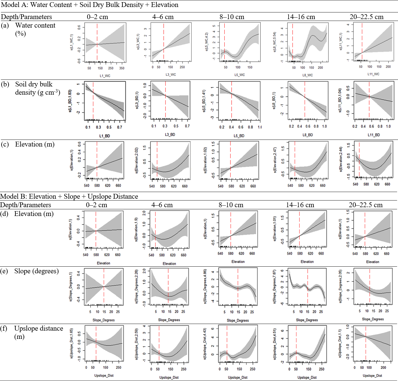
Figure 13 GAM smooth function outputs at five depth layers for the parameters in the two best-performing models. The x axis on each plot is the model predictor and its real value range. The y axis is the smoothing parameter, s(covariate, degree of freedom). Vertical dashed red lines indicate a point at which the smoothing parameter is the zero residual point.

For each plot in Fig. 13, the x axis is the model predictor and its value range, and the y axis is the smoothing parameter. The numbers on the y axis indicate the partial residuals from the fit. Thus, the y axis demonstrates an increase or decrease of the response values against its predicted mean. The gray area represents the 95 % confidence interval range, and the vertical dashed red line indicates the predictor value at which the smoothing parameter is zero mean.

The fitted curves for Model A (fitted smooth) show that water content and elevation were positively related to Cs-137 (Fig. 13a and c). Soil dry bulk density was negatively related to Cs-137 (Fig. 13b). Cs-137 increases as water content increases, although the increasing pattern is not linear in two depth intervals (Fig. 13a). The Cs-137 increases above the mean at around the water content 50 %–120 %. The samples in this study contained soils with mass water content above 100 %, and those soils had elevated Cs-137, when they were dried. Cs-137 decreased below the mean at a soil dry bulk density around 0.2–0.55 g cm⁻³ (Fig. 13b). GAMs returned higher explanation percentages when run against Cs-137 in Bq kg⁻¹ unit than in Bq m⁻² (Tables 4 to 6). These results indicated that soil dry bulk density, included in mass depth (Bq m⁻²) calculation, was not a significant factor in explaining Cs-137 concentrations. The model-fitted curves in Fig. 13b show the negative linear relationships between soil dry bulk density and Cs-137 predictions. Since soil dry bulk density increases with depth, Cs-137 is concentrated in low-density soils close to the surface. In this study site, soil dry bulk density had an influence on Cs-137 concentrations, which appeared when density was combined with other model parameters. Cs-137 and elevation showed positive linear correlations or U-shaped fitted curves depending on the depth (Fig. 13c). The bottom of the U shape was around the elevation of 610 m. One sample collected at the elevation of 613 m contained the highest core average soil dry bulk density, which also had the lowest core total Cs-137 concentration and the highest dry bulk density in the top 0–2 cm layer.

The fitted curves for Model B show that elevation was positively related to Cs-137 (Fig. 13d), and slope was negatively related to Cs-137 except in the 0–2 cm depth (Fig. 13e). Elevation was a common predictor in both models (Fig. 13c and d). The elevation's fitted curves in the two models showed that the same predictor's fitted smooths could vary depending on its relation to other predictors in the model. Slope showed a fitted curve near the surface (0–2 cm depth) with an increasing trend, but an opposite trend from other layers below (Fig. 13e). Three samples with the highest Cs-137 concentrations in the 0–2 cm depth were found at slopes steeper than 15^∘. These samples pushed the trend upwards toward a steeper slope in the 0–2 cm depth range. Slope presented the fitted curves with multiple knots between 5–25^∘ in the 14–16 cm depth. Yet, the fitted smooths did not move away from the mean, indicating that slope in this range contributed little to Cs-137 concentration. Upslope distance contributed to a Cs-137 increase toward the shortest upslope distance (at the ridge area) and the longest upslope distance (hill bottom area; Fig. 13f). The sample with the highest core total Cs-137 concentration was about 10 m below the ridge edge. Higher Cs-137 concentrations at the ridge area is counter-intuitive because Cs-137 was expected to move downslope with surface soil creep or runoff. The Cs-137 concentrations in five samples collected at the shortest upslope distances did not show any apparent relationships with water content, soil dry bulk density, or other topographic features.

On the basis of the model fits, predictions for the Cs-137 concentrations in this study site are as follows.

1. Cs-137 concentrations generally increase with elevation, but the increase is not linear (Figs. 7 and 13c).

2. Higher Cs-137 concentrations can be found at the highest elevation near the ridge or hill bottom (Fig. 13c and f).

3. Higher Cs-137 concentrations will be observed at the locations with lower slopes, which could include flat areas at the ridge and near the hill bottom (Fig. 13e).

4. Soils with higher water content might contain higher Cs-137 concentrations once they are dried (Fig. 13a).

5. Higher Cs-137 concentrations can be found in lower soil dry bulk density close to the surface. Exceptions can be found at locations where water does not pond, even though soil dry bulk density is higher (Fig. 13b and c).

4.3 The effect of DEM resolution

The ratios between topographic parameter values extracted from the two DEMs are shown in Table 8. The last column of Table 8 indicates the DEM resolution where each topographic parameter appeared in the best-performing GAM models (Table 6). The elevation and slope values were consistent between the 1 and 10 m DEM, indicating that elevation did not change drastically over distances less than 10 m. Upslope distance had the largest difference between the DEMs. Plan curvature and TWI, which influence surface water ponding, appeared in the best-performing models with the 1 m DEM. Upslope distance performed better with the 10 m DEM, but the average upslope distance was 4 times greater with the 10 m DEM.

Table 8 Topographic value difference ratio between the 1 and 10 m resolution DEMs (medians). The right column shows with which DEM, 1 or 10 m, each topographic parameter appeared in the best-performing model.

4.4 Study contribution

This study employed empirical approaches to derive predictive relationships among Cs-137 and soil property data and local topography. The statistical results show the power of detecting co-functionalities of topographic predictors on Cs-137 accumulations on the ground surface and with depth, which could enhance the understanding of the geomorphic mechanisms governing Cs-137 accumulations in a forested area. While model prediction errors might depend heavily on factors not included in this study, the current approach proposes a methodology to partition observed Cs-137 concentrations into explainable and unexplainable portions. The methodology and results presented here could contribute to ongoing research on understanding the distribution of radioactive contamination in complex terrains.

4.5 Study limitations

In this study, the Cs-137 measurement began in 2016, and the physical translocation of Cs-137 prior to 2016 was not considered as no soil monitoring was conducted. The only data available were the initial Cs-137 deposition estimates from the Japanese government and the US Department of Defense (MEXT, 2011), which was 1000–3000 kBq m⁻² as of July 2011. The Cs-137 values are decay normalized and do not consider the physical movement of Cs-137 over the 3-year sampling period. While the effects of precipitation magnitude and frequency cannot be ignored, all soil sampling campaigns were conducted at approximately the same time of year (i.e., after the rainy season). All sampling campaigns avoided intense precipitation immediately prior to sample collections.

5 Conclusions

Following an earthquake near the northeast coast of Honshu, Japan, and a subsequent tsunami, the FDNPP suffered a catastrophic failure and a radioactive plume, including Cs-137, was released into the atmosphere. While much previous research focused on documenting Cs-137 concentrations in nearby environments, there has been no systematic and quantitative study that examined the effect of topographic indices and soil properties on the concentration and distribution of Cs-137 from this accident. To address this issue, 58 soil core samples were collected over a 3-year period from the ground surface to depths of 30 cm in Iitate village, a forested region located 35 km northwest of the FDNPP. The Cs-137 concentrations for these samples were assessed along with various topographic indices derived from digital elevation models and soil properties. Generalized additive models (GAMs) were then employed to quantitatively determine the singular and collective impact of topography, soil properties, and digital elevation model resolution on predicting the concentration of Cs-137 within this landscape. The primary conclusions of the study are as follows.

1. In general, Cs-137 activities were highest near the ground surface and decreased exponentially with depth. The average depth of 90 % concentration was 6.1 cm in kBq kg⁻¹ and 6.9 cm in kBq m⁻², and the average migration depth for all samples was 21.7 cm.

2. Higher concentrations of Cs-137 occurred at the highest elevations or near the bottom of hills.

3. Elevation, slope, upslope distance, plan curvature, and TWI were derived for each sample location using 1 and 10 m DEMs. Resolution of the DEM produced marked differences in the upslope distance, plan curvature, and TWI indices determination, which then affected the Cs-137 predictions.

4. Using two units for Cs-137 concentration, five topographic indices, and two soil properties, 63 GAMs were evaluated using one- to three-parameter combinations and two DEMs with different resolutions, which were assessed using several criteria. For the single-parameter models, none returned average deviance-explained percentages greater than 36 %. In contrast, the most effective model combinations for predicting Cs-137 deviance were “water content + bulk density + elevation” for the 1 m (53.56 %) and 10 m (54.03 %) DEMs, given the empirical data reported herein. The most effective topographic parameter combinations were “slope + plan curvature + TWI” when using the 1 m DEM (40.62 %) and “elevation + slope + upslope distance” when using the 10 m DEM (46.70 %). Concentrations of Cs-137 within this landscape were reverse-predicted using the best two GAMs (Model A: “water content + bulk density + elevation” and Model B: “elevation + slope + upslope distance”). For the data reported herein, Model A outperformed Model B.

While this study focused on a small forested region affected by the FDNPP accident, the results clearly show that Cs-137 concentrations in soils are strongly affected by landscape topography. This topographic effect should be given careful consideration in the use of anthropogenic radionuclides as environmental tracers and in the assessment of current and future environmental risks due to nuclear power plant accidents.

Appendix A: Equations

A1 R package mgcv GAM model settings

Model ← gam(Cs-137 ∼ $s\left(x_{\mathrm{1}}\right)+s\left(x_{\mathrm{2}}\right)+s\left(x_{\mathrm{3}}\right)$, data = data, method = “REML”, bs = “cr”, family = Gamma(link = log)), where “s” is a smooth function of covariates of the predictor, “method” specifies a fitting method, and “bs” specifies basis function (“cr”, cubic splines, in this model). “family” specifies a response variable distribution type. Here, “link” solves the problem of using linear models with non-normal data by linking the estimated fitted values to the linear predictor (Clark, 2013). This study used “Gamma(link = log)” to address complex, non-linear interactions among predictors.

A2 Cs-137 decay equations

The Cs-137 decay constant is calculated as follows (Eq. A1):

$$\begin{array}{}\text{(A1)}& \mathit{\lambda }={\displaystyle \frac{\ln \mathrm{2}}{T\frac{\mathrm{1}}{\mathrm{2}}}},\end{array}$$

where λ is the decay constant and $T_{\mathrm{1}/\mathrm{2}}$ is the half-life. The half-life of Cs-137 is 30.17 years; thus, λ=0.023 yr⁻¹. The radioactive decay formula is as follows (Eq. A2):

$$\begin{array}{}\text{(A2)}& N_{\mathrm{0}}={\displaystyle \frac{N_t}{e-\mathit{\lambda }t}},\end{array}$$

where N₀ is the original Cs-137 value, N_t is the Cs-137 value after time t, and λ is the decay constant (IAEA-TECDOC, 2003).

A3 Akaike information criterion (AIC)

$$\begin{array}{}\text{(A3)}& \mathrm{AIC}=-\mathrm{2}l\left(\widehat{\mathit{\theta }}\right)+\mathrm{2}p(\mathrm{Wood},\mathrm{2017}),\end{array}$$

where $l\left(\widehat{\mathit{\theta }}\right)$ is log likelihood and p is the number of identifiable model parameters (usually, the dimension of θ).

A4 Generalized cross validation (GCV)

$$\begin{array}{}\text{(A4)}& V_{\mathrm{g}}={\displaystyle \frac{n\sum _{i=\mathrm{1}}^n{\left(y_i-{\widehat{f}}_i\right)}^{\mathrm{2}}}{[n-\mathrm{tr}(A){]}^{\mathrm{2}}}}(\mathrm{Hastie}\mathrm{et}\mathrm{al}.,\mathrm{2009};\mathrm{Wood},\mathrm{2017}),\end{array}$$

where V_g is the generalized cross-validation score, y_i is the excluded data, $\widehat{f}$ is the estimate from fitting to all the data, and tr(A) is the mean of the model matrix A_ii. The matrix measures the degree that the ith datum influences the overall model fit.

A5 Cook's outliers

$$\begin{array}{}\text{(A5)}& \begin{array}{rl}{D}_i=& {\displaystyle \frac{{\left({\widehat{\mathit{\beta }}}_{(-i)}-\widehat{\mathit{\beta }}\right)}^{\prime }X\sim X\left({\widehat{\mathit{\beta }}}_{(-i)}-\widehat{\mathit{\beta }}\right)}{(p+\mathrm{1}){\widehat{\mathit{\sigma }}}^{\mathrm{2}}}}i=\mathrm{1},\mathrm{2},\mathrm{\dots }n\\ & (\mathrm{Cook},\mathrm{1977};\mathrm{Stevens},\mathrm{1984}),\end{array}\end{array}$$

where $\widehat{\mathit{\beta }}$ is the vector of estimated regression coefficients with the ith data point deleted, p is the number of predictors, ${\widehat{\mathit{\sigma }}}^{\mathrm{2}}$ is the residual variance of the full dataset.

Appendix B: Summary of all primary data collected

Table B1 Summary of topographic indices for all core sample locations (58 core samples, 46 locations).

Table B2 Summary of data collected for all core sample locations. Units include Cs-137: Bq kg⁻¹, dry bulk density: g cm⁻³, mass water content: %, sand, silt, and clay content: %. Among 58 core samples, multi-year samples were decay normalized and averaged.