the Creative Commons Attribution 4.0 License.
the Creative Commons Attribution 4.0 License.
 | 03 Aug 2021
Topographic disequilibrium, landscape dynamics and active tectonics: an example from the Bhutan Himalaya
Timothée Sassolas-Serrayet
Rodolphe Cattin
Romain Le Roux-Mallouf
Matthieu Ferry
Dowchu Drukpa
The quantification of active tectonics from geomorphological and morphometric approaches commonly implies that erosion and tectonics have reached a certain balance. Such equilibrium conditions are however rare in nature, as questioned and documented by recent theoretical studies indicating that drainage basins may be perpetually re-arranging even though tectonic and climatic conditions remain constant. Here, we document these drainage dynamics in the Bhutan Himalaya, where evidence for out-of-equilibrium morphologies have for long been noticed, from major (> 1 km high) river knickpoints and from high-altitude low-relief regions in the mountain hinterland. To further characterize these morphologies and their dynamics, we perform field observations and a detailed quantitative morphometric analysis using χ plots and Gilbert metrics of drainages over various spatial scales, from major Himalayan rivers to their tributaries draining the low-relief regions. We first find that the river network is highly dynamic and unstable, with much evidence of divide migration and river captures. The landscape response to these dynamics is relatively rapid. Our results do not support the idea of a general wave of incision propagating upstream, as expected from most previous interpretations. Also, the specific spatial organization in which all major knickpoints and low-relief regions are located along a longitudinal band in the Bhutan hinterland, whatever their spatial scale and the dimensions of the associated drainage basins, calls for a common local supporting mechanism most probably related to active tectonic uplift. From there, we discuss possible interpretations of the observed landscape in Bhutan. Our results emphasize the need for a precise documentation of landscape dynamics and disequilibrium over various spatial scales as a first step in morpho-tectonic studies of active landscapes.
- Article
(28400 KB) - Full-text XML
-
Supplement
(6579 KB) - BibTeX
- EndNote


The morphology of the Earth's surface and its evolution in space and time result from the competition and balance between tectonics and surface processes. The interplay between these processes, with erosion followed by transport and deposition of the produced sediments in subsiding basins, leads to a continuous dynamic redistribution of masses, eventually modulated by climate (e.g., Allen, 2008). In erosive systems, such as in uplifting and growing mountain ranges, such physical competition between uplift and erosion theoretically leads to steady state after a characteristic time that mostly depends on the erosional efficiency (e.g., Whipple and Tucker, 1999; Willett et al., 2001; Bonnet and Crave, 2003; Whipple and Meade, 2004, 2006; Simoes et al., 2010). This concept of steady state and equilibrium between tectonics and erosion provides an effective conceptual framework, commonly used for investigating and quantifying active tectonics from geomorphology (e.g., Lavé and Avouac, 2001). However, topographic equilibrium may only be reached at a regional scale (Willett and Brandon, 2002) and is expected not to be achieved at the more local scale of the drainage network even though tectonic and climatic boundary conditions remain constant, as illustrated by numerical (e.g., Sassolas-Serrayet et al., 2019) or analog (e.g., Hasbargen and Paola, 2000) models. The dynamics of the river network are expected to be even more pronounced in natural landscapes for which boundary and forcing conditions vary over time and space. In fact, the formalism used in earlier theoretical studies to model erosion is oversimplified as it does not capture the complex 3D dynamic response of drainage basins, in particular through the constant mobility of drainage divides (e.g., Goren et al., 2014; Willett et al., 2014). An example of such landscape dynamics during mountain-building lies in the progressive capture of longitudinal drainages by steeper transverse rivers, as exemplified in the field (e.g., Babault et al., 2012), in analog models (Viaplana-Muzas et al., 2015), or in the dynamic re-organization of the river network as a response to tectonic stresses (e.g., Castelltort et al., 2012; Guerit et al., 2018). River captures were also evidenced in old orogens where topographic equilibrium is hypothesized (Prince et al., 2011). This mobility of drainage divides leads to a lengthening of the time needed to reach theoretical steady state and generates a potential perpetual transience of landscapes (e.g., Hasbargen and Paola, 2000; Yang et al., 2015; Whipple et al., 2017b). It is expected to generate variations in the sedimentation rates at river outlets by modifying the sediment routing system (e.g., Viaplana-Muzas et al., 2019) and to elucidate observed large dispersions in denudation rates, even in regions that are believed to be in quasi-topographic steady state (Willett et al., 2014; Beeson et al., 2017; Sassolas-Serrayet et al., 2019). Interestingly, this dispersion in measured denudation rates increases most often for smaller drainage basins, further emphasizing that the concept of steady state is highly scale-dependent as variations related to the local mobility of drainage divides average out at the scale of large river basins (Matmon et al., 2003; Sassolas-Serrayet et al., 2019).
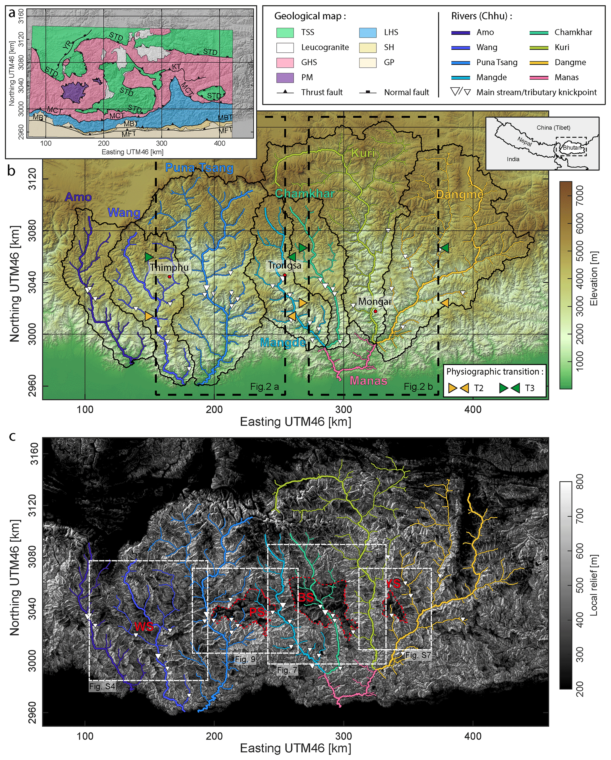
Figure 1Topography, relief and geology of Bhutan. (a) Geological map of Bhutan, after Greenwood et al. (2016). Main tectono-stratigraphic units are from south to north: the Gangetic Plain (GP), the Siwaliks Hills (SH), the Lesser Himalayan Sequence (LHS) including the Paro metasediments (PM) in western Bhutan, the Greater Himalayan Sequence (GHS) including some leucogranites, and the Tethyan Sedimentary Series (TSS). These units are separated by major tectonic contacts, which are from north to south: the Main Frontal Thrust (MFT), the Main Boundary Thrust (MBT), the Main Central Thrust (MCT), and the South Tibetan Detachment (STD). Locally, some other contacts have been described such as the Kakhtang Thrust (KT) in north-eastern Bhutan. To the north-west of Bhutan, north of the High Himalayan range, the Yadong Rift (YR) is part of the southern Tibetan grabens. The extension of the geological map is reported over the shaded topographic map of (b). (b) Topographic map of Bhutan, from ALOS World 3D – 30 m (AW3D30) DEM data. Main drainage basins are delineated by black lines, and associated main rivers are color-coded and labeled. Thick colored lines correspond to the main trunk rivers, while thinner lines indicate main tributaries. Major knickpoints are also reported along trunk and tributary rivers. Dashed rectangles locate the swath profiles of Fig. 2a and b. Orange and green arrows on the side of these rectangles locate physiographic transitions T2 and T3 as placed in Fig. 2a and b. Inset denotes the location of the topographic map with respect to regional political borders. (c) Map of local relief, as calculated from the topography shown in (b), with a moving window of 500 m. Major high-altitude low-relief areas are manually delineated by dashed red lines. These are from west to east: the Phobjikha (PS), the Bumthang (BS), and the Yarab (YS) surfaces. In western Bhutan, another region of lower relief is also found in the Bhutan hinterland along the Wang Chhu and Amo Chhu, even though less well defined than the others: the Wang surface (WS). From west to east, dashed rectangles locate the extension of Figs. S4, 9, 7 and S7 (Figs. S4 and S7 in the Supplement).
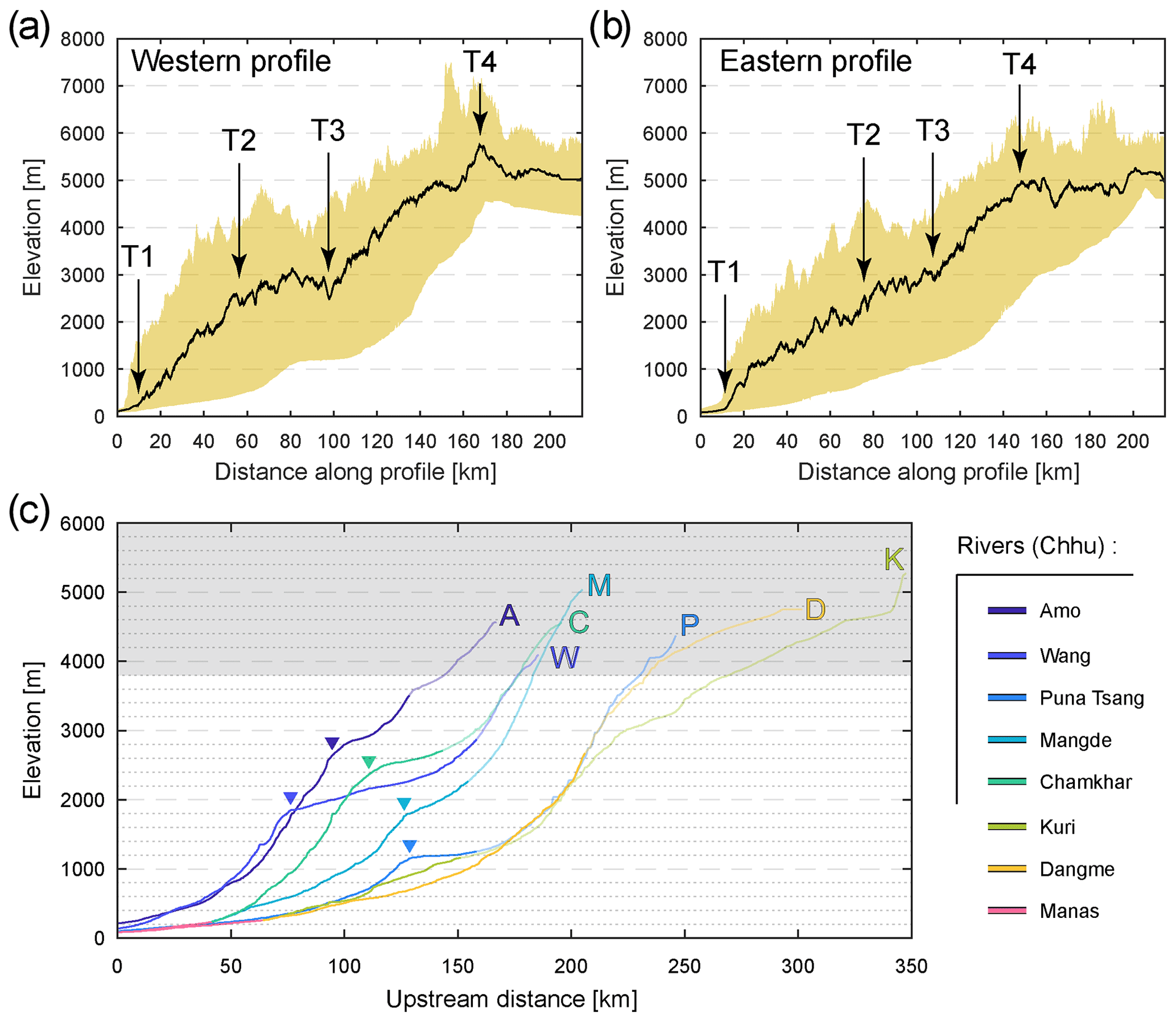
Figure 2Topographic and longitudinal river profiles. (a, b) Swath topographic profiles across the western (a) and eastern (b) Bhutan Himalaya over a 100 km wide region, from the Gangetic Plain up to the southern Tibetan Plateau. Location of the swaths is reported in Fig. 1b. The colored area encompasses the whole range of altitude values, while the black line draws the median altitude across the profiles. Major physiographic transitions, labeled T1 to T4, are also reported. (c) Longitudinal profiles of major and large rivers in Bhutan, illustrating the variety of river profiles. Rivers are located on the maps of Fig. 1 and are here color-coded and labeled. Major knickpoints are also pointed by triangles. Regions with altitudes above 3800 m (grey area) are not to be compared directly to the downstream sections, as these may have a glacial imprint. Portions of the rivers north of physiographic transition T3 are reported by transparent segments. A: Amo Chhu; M: Mangde Chhu; C: Chamkhar Chhu; W: Wang Chhu; P: Puna Tsang Chhu; D: Dangme Chhu; K: Kuri Chhu.
Here, we propose to further investigate these questions, mostly derived from theoretical studies or in few field cases, by considering the emblematic natural example of the Himalayan range in Bhutan (Fig. 1). Because of their high rates of continental deformation and erosion, the Himalayas have for long been an ideal natural case for exploring the interactions between tectonics and surface processes, as well as the associated landscape response (e.g., Beaumont et al., 2001; Lavé and Avouac, 2001; Burbank et al., 2003; Godard et al., 2004, 2014; Hodges et al., 2004; Thiede et al., 2004, 2005; Grujic et al., 2006; Clift et al., 2010; Adlakha et al., 2013). In particular, the Himalayas of central Nepal have been considered the archetype of a topography equilibrated on average, from their concave topography and hypsometry (Duncan et al., 2003) or from the observed consistency between denudation (Godard et al., 2014), incision (Lavé and Avouac, 2001) and exhumation (e.g., Bollinger et al., 2006) rates over various spatial and temporal scales. Such is not the case further east, in Bhutan, where evidence for out-of-equilibrium morphologies has for long been noticed, from the convex topographic profile (Fig. 2a and b) and from high-altitude low-relief regions (Fig. 1c) and major knickpoints (Fig. 2c) within the mountain hinterland (Duncan et al., 2003; Baillie and Norbu, 2004; Grujic et al., 2006; Adams et al., 2015, 2016). These morphological features have been interpreted in a variety of ways, mostly as reflecting either climatic (Grujic et al., 2006) or tectonic (Baillie and Norbu, 2004; Coutand et al., 2014; Adams et al., 2016) changes or, in other words, as representing the landscape transience towards a new equilibrium state. However, recent findings in other contexts question these interpretations: low-relief landscapes were shown to form possibly dynamically in situ as a response to an increase in local base level (e.g., Babault et al., 2007) or to a persistent drainage re-organization even in the case of constant tectonics and climate (Yang et al., 2015). Finally, despite these observations in Bhutan and the questions they raise, denudation rates have been regarded as reflecting uplift rates and used to derive the geometry of the underlying main active fault (Le Roux-Mallouf et al., 2015) or the timing of interpreted recent tectonic changes (Adams et al., 2016). Whether or not these denudation rates are indeed representative of actual uplift rates needs to be probed. Because smaller drainage basins are the most inclined to have denudation rates deviating from uplift rates in the case of disequilibrium (Sassolas-Serrayet et al., 2019), the answer to this question is intuitively dependent on the size and location of the sampled drainage basins within the overall drainage system.
To explore the landscape dynamics of the Bhutan Himalaya as well as their spatial and temporal characteristics, we hereafter conduct a detailed morphometric analysis of this particular field example. We use χ plots (Perron and Royden, 2013) and Gilbert metrics (Whipple et al., 2017b; Forte and Whipple, 2018) for drainages of various dimensions, from major Himalayan rivers to more local tributary streams draining high-altitude low-relief regions. Our analysis does not reveal any evidence for a general wave of incision migrating upstream the drainage network. Instead, we find ample evidence for a high instability of the river network at various spatial scales that has not been documented yet, with migrating drainage divides and numerous captures. The co-location and spatial organization of all geomorphic features along a longitudinal swath, whatever the considered spatial scale and the dimensions of the investigated drainage basins, calls for a common local origin and support of the observed landscape dynamics, most probably related to active uplift in the mountain hinterland as proposed in some earlier studies. Finally, we discuss the implications of our findings, in particular in terms of how elevated low-relief regions may have formed and in terms of relative timescales of landscape response to network re-organizations.
2.1 Geological setting
One of the main characteristics of the Himalayan arc is its structural and tectono-stratigraphic continuity over ca. 2500 km (e.g., Gansser, 1964, 1983; McQuarrie et al., 2008). From south to north, and therefore from the Gangetic Plain in the foreland to southern Tibet, major tectonic contacts are the Main Frontal Thrust (MFT), the Main Boundary Thrust (MBT), the Main Central Thrust (MCT) and the South Tibetan Detachment (STD). The un-metamorphosed synorogenic detrital series of the Siwaliks Group (e.g., Gautam and Rösler, 1999; Coutand et al., 2016) are thrusted over the Gangetic Plain along the MFT, which stands as the southern deformation front of the orogen. The Lesser Himalayan series are thrusted over the Siwaliks molasses along the MBT. These series are formed of metasediments, initially deposited on the Indian margin during the Proterozoic and Paleozoic (e.g., Upreti, 1999; Long et al., 2011b, and references therein), and subsequently deformed, metamorphosed and exhumed since the Mid–Late Miocene, mostly in the form of duplexes in the mountain hinterland (e.g., Schelling and Arita, 1991; DeCelles et al., 2001; Huygue et al., 2001; Robinson et al., 2001; Bollinger et al., 2004, 2006; Long et al., 2012). Further north, the Greater Himalayan Sequence is thrusted over the Lesser Himalaya along the MCT. This sequence is constituted of granulites and ortho- and para-gneisses of the former Indian margin, with widespread leucogranites (e.g., Le Fort et al., 1987; Guillot and Le Fort, 1995). The MCT stands as a thick top-to-the-south shear zone, active by Early to Mid-Miocene (e.g., Tobgay et al., 2012, and references therein), and subsequently deformed by the duplexes of the Lesser Himalayan series. Finally, the Tethyan Sedimentary Sequence is formed of the sedimentary cover of the northern Indian margin (e.g., Liu and Einsele, 1994); it is separated from the high-grade Greater Himalayan rocks by the top-to-the-north normal STD. Except for the un-metamorphosed Siwaliks, the erodibility of the series present throughout the mountain range is found to be relatively comparable (Lavé and Avouac, 2001; Adams et al., 2020).
The Bhutan Himalaya obeys this general tectonic and stratigraphic organization observed throughout the Himalayan arc (Fig. 1a), even though presenting some peculiarities and specificities (Gansser, 1983; Long et al., 2011a; Greenwood et al., 2016). In particular, the Greater Himalayan and the Tethyan Sedimentary sequences are here much more exposed throughout the mountain belt when compared to the Himalayas of central Nepal where these sequences are only preserved in the form of individual klippen (e.g., Duncan et al., 2003). In turn, Lesser Himalayan series mostly crop out along the main topographic mountain front, or within structural windows, such as the Paro window in western Bhutan (Tobgay et al., 2012) or the larger Lesser Himalayan window along the Kuri Chhu in eastern Bhutan (Long et al., 2011b) (Fig. 1a). Because of the limited flexural subsidence in the broken foreland of Bhutan (Verma and Mukhopadhyay, 1977; Hammer et al., 2013), most probably related to the presence of the Shillong Plateau basement high further south (e.g., Biswas et al., 2007; Clark and Bilham, 2008; Yin et al., 2010), the Siwaliks series is here much less developed than elsewhere along the Himalayan arc (Hirschmiller et al., 2014), and the MFT is even absent in western Bhutan (Long et al., 2011a; Greenwood et al., 2016) (Fig. 1a).
All major thrust faults are interpreted to branch off the Main Himalayan Thrust (MHT) at depth, which stands as the main crustal-scale detachment at the base of the Himalayan orogenic wedge (e.g., Schelling and Arita, 1991; DeCelles et al., 2001). Overall, the geometry of the MHT appears quite simple, with the frontal emerging ramp of the MFT, rooting at depth into a wide shallowly north-dipping structural flat, and pursuing northward down to a mid-crustal ramp beneath the High Himalayan range. This general structure has been proposed throughout the Himalayas, in particular in Nepal (e.g., Lyon-Caen and Molnar, 1983, 1985; Schelling and Arita, 1991; Lavé and Avouac, 2001; Bollinger et al., 2004) but also more recently suggested in Bhutan, as imaged from geophysics (Diehl et al., 2017; Singer et al., 2017), or evidenced from the modeling of interseismic strain (Marechal et al., 2016), thermochronological data (Coutand et al., 2014) or denudation rates (Le Roux-Mallouf et al., 2015). In the details, the flat structure connecting both the frontal and the mid-crustal ramps could be locally more complex with secondary ramps (e.g., DeCelles et al., 2001; McQuarrie et al., 2008; Adams et al., 2016; Hubbard et al., 2016).
The Himalayan range is actively absorbing shortening, with rates increasing eastwards from ca. 13 to ca. 21 mm yr−1 along the arc (Stevens and Avouac, 2015). Active tectonics are manifested by numerous historical earthquakes all along the Himalayan arc in addition to paleoseismological evidence of major earthquakes rupturing the MHT up to the surface (e.g., Bilham, 2019, and references therein). Even though much less investigated, the Bhutan Himalaya is also seismically active (Drukpa et al., 2006). It was struck by a major historical earthquake in 1714 (e.g., Hetenyi et al., 2016), in addition to other past events recently revealed in geomorphological and paleoseismological studies along the frontal MFT–MBT thrust system (Berthet et al., 2014; Le Roux-Mallouf et al., 2016, 2020).
2.2 Geomorphology of Bhutan: general characteristics
The topography of the Bhutan Himalaya is characterized by a convex profile, with four major physiographic transitions, hereafter referred to as T1 to T4 from south to north (modified after Duncan et al., 2003; Baillie and Norbu, 2004; Adams et al., 2013) (Fig. 2a and b). The first one (T1) corresponds to the rise of the mountain topographic front above the Gangetic Plain. Northward, topography increases continuously up to ca. 3000 m on average for the first ca. 70–80 km (T2), then remains constant on average and high, increases again after ca. 100–125 km (T3) and reaches average values of ca. 5000 m by ca. 175 km (T4) and northwards (Fig. 2a and b). Except for T2, these physiographic transitions are also observed in central Nepal, where the abrupt topographic rise between T3 and T4 has been interpreted as related to the uplift of the High Himalayan range above the mid-crustal ramp of the MHT (e.g., Lyon-Caen and Molnar, 1983, 1985; Cattin and Avouac, 2000; Lavé and Avouac, 2001; Bollinger et al., 2006). This interpretation is also expected to hold in Bhutan, as this elevation ascent coincides spatially with the location of the recently evidenced mid-crustal ramp (Coutand et al., 2014; Marechal et al., 2016; Diehl et al., 2017; Singer et al., 2017) – or possibly slightly deported south of this ramp (Le Roux-Mallouf et al., 2015).
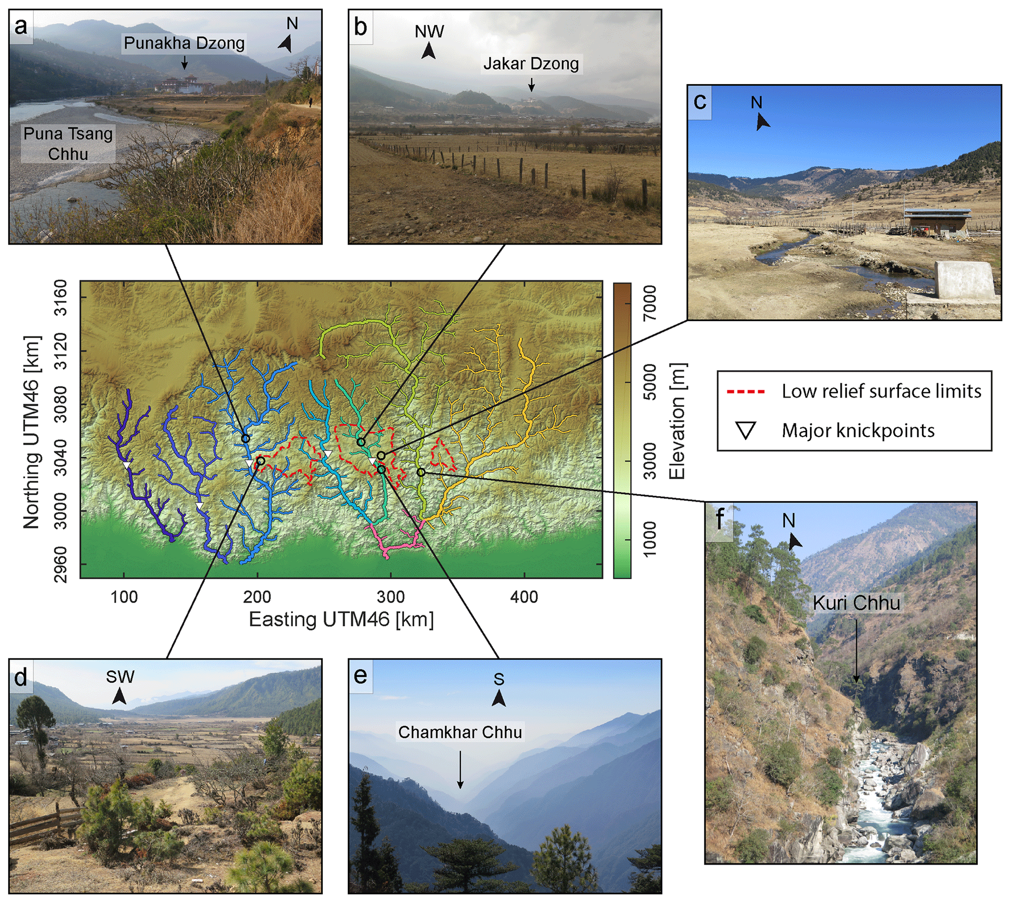
Figure 3Field pictures representative of the various landscapes in the hinterland of the Bhutan Himalaya. Topographic map in the center locates field pictures relative to low-relief regions (contoured with red dashed line) and to major knickpoints along rivers (rivers color-coded as in Figs. 1 and 2). (a) Alluvial plain along the Puna Tsang Chhu, upstream of its major knickpoint. Picture taken near the Dzong of Punakha. (b) Alluvial plain along the Chamkhar Chhu (Bumthang surface), upstream of its major knickpoint. Picture taken near Jakar. (c) High-altitude low-relief area of Ura (south-easternmost portion of the Bumthang surface). (d) High-altitude low-relief area of Kotakha (westernmost portion of the Phobjikha surface). (e) Deep gorge south of the major knickpoint along the Chamkhar Chhu. (f) Canyon along the Kuri Chhu.
The abrupt topographic rise from T1 to T2 and the high-altitude region between T2 and T3 are mostly specific to the landscape of the Bhutan Himalaya along the Himalayan arc (Duncan et al., 2003; Adams et al., 2013). The region between T2 and T3 is characterized by a locally relatively lower relief (Figs. 1c and 3a–d), in contrast to what is observed further south from T1 to T2 (Fig. 3e and f) but also further north from T3 to T4 where high-elevation crests are flanked by deep gorges (Duncan et al., 2003; Baillie and Norbu, 2004; Grujic et al., 2006; Adams et al., 2015, 2016) (Fig. 1). More precisely, these lower-relief regions may correspond either to high-elevation regions around low-relief alluvial valleys drained by major rivers (e.g., the Wang and Bumthang regions traversed by the Wang Chhu and Chamkhar Chhu, respectively) (Figs. 1c and 3a and b) or to smaller elevated low-relief landscape patches connected to the main drainage network through tributary streams (e.g., Phobjikha or Yarab surfaces) (Figs. 1c and 3c and d). These valleys or surfaces are characterized by well-developed soils with saprolite horizons and locally contain bogs (Baillie et al., 2004; Adams et al., 2016). It should be noted that high-elevation low-relief alluvial valleys found along some of the Himalayan rivers (Fig. 3a and b) act as local base levels for upstream erosion.
Major rivers in Bhutan have their sources along the southern flank of the High Himalayan peaks, except for the trans-Himalayan Kuri Chhu and Dangme Chhu to the east, and to some extent the Amo Chhu to the west, whose headwaters are located within southern Tibet. These rivers are characterized by a variety of profiles (Baillie and Norbu, 2004), but most of them have significant knickpoints, in some cases of the order of – or higher than – ca. 1 km (Fig. 2c). These knickpoints occur at the head of gorges flowing through low-relief landscapes or immediately downstream of them (Baillie and Norbu, 2004; Adams et al., 2016) (Figs. 1 and 3e). They separate rivers in two main segments (Fig. 2c): river profiles are steep downstream of these knickpoints, while upstream river portions have alluvial fills (Fig. 3a and b) and are located in the low-relief portions of the mountain range, north of T2.
Present-day glacial valleys and cirques are mostly restricted to altitudes higher than ca. 4200 m (Iwata et al., 2002) and are generally located either near T2 or mostly north of T3. Glaciers likely advanced and expanded to altitudes of ca. 3800 m during the Holocene and Pleistocene (Iwata et al., 2002; Meyer et al., 2009). There is no evidence for glacial imprint on the high-altitude low-relief landscapes investigated here, except locally along some of the southern edges of low-relief areas where altitudes reach ca. 4000 m (Adams et al., 2016).
2.3 Geomorphology of Bhutan: previous interpretations
By comparing the morphology and geology of these two regions of the Himalaya, Duncan et al. (2003) proposed that topographic and morphologic differences between central Nepal and Bhutan could be related to an along-strike tectonic segmentation of the Himalayan range and to the associated variable balance between uplift and erosion, in which the timing of large-scale deformation and uplift would be younger in Bhutan. This interpretation of a less mature landscape would be supported by the extensive exposure of Great Himalayan and Tethyan sequences in Bhutan (e.g., Gansser, 1983; Long et al., 2011a; Greenwood et al., 2016) (Fig. 1a), which contrasts with the klippen of central Nepal (e.g., Gansser, 1964; Schelling and Arita, 1991; DeCelles et al., 2001; Bollinger et al., 2004). Lateral variations in the timing of major fault systems along the Himalayan arc cannot be excluded, such as for the Main Central Thrust by the Early to Mid-Miocene (e.g., Tobgay et al., 2012, and references therein) or for the exhumation of the Lesser Himalayan sequences since the Late Miocene (e.g., Huygue et al., 2001; Robinson et al., 2001; Bollinger et al., 2006; Long et al., 2012, and references therein). However, such interpretation would first require that the large-scale landscape response time be much greater than what could be justifiable given the regional high erosion rates (e.g., Lavé and Avouac, 2001). Also, in this case, erosion rates in Bhutan would be expected to have increased in recent geological times, as a response to balance uplift. However, thermochronological data rather suggest a general decrease in exhumation rates over the last 4–6 Myr (Grujic et al., 2006; Coutand et al., 2014; Adams et al., 2015).
This general decrease in exhumation rates since Late Miocene –Early Pliocene has been invoked by Grujic et al. (2006) to be related to the rain shadow generated by the coeval topographic rise of the Shillong Plateau further south in the foreland of Bhutan (e.g., Biswas et al., 2007; Clark and Bilham, 2008; Govin et al., 2018; Rosenkranz et al., 2018, and references therein). Such rain shadow would have led to lower erosion rates and from there to locally increased relief and elevation by modifying the balance between uplift and erosion. Following this idea, high-altitude low-relief regions in Bhutan would be relict landscapes of prior wetter conditions. However, as noticed by Baillie and Norbu (2004), the rain shadow by the Shillong Plateau is relative as climatic conditions are everywhere wet and tropical in Bhutan (Bookhagen and Burbank, 2006). Some variations exist along the foothills, with modern precipitation rates peaking to more than 6 m yr−1 on average in between physiographic transitions T1 and T2, but climatic conditions are then relatively constant northward within the range interior (north of T2). Also, low-relief regions are mostly found within the western half of Bhutan (Fig. 1c), where the Shillong rain shadow is supposedly lowest or inexistent according to Grujic et al. (2006).
In addition to these general observations on the overall topography or the presence of low-relief areas in the range interior, Baillie and Norbu (2004) noticed the variety of river profiles (Fig. 2c), despite overall similar climatic and lithologic conditions along Bhutan and from there suggested that these morphologies be mostly related to lateral differential tectonics, accommodated by north–south faulting. However, such laterally variable uplift should produce a significant along-strike variability in exhumation rates, a pattern not seen in thermochronological data (Grujic et al., 2006; Coutand et al., 2014; Adams et al., 2015). Indeed, most significant variations in exhumation rates are across-strike and not along-strike and should relate to cross-sectional changes in the geometry of the underlying Main Himalayan Thrust (Coutand et al., 2014; Le Roux-Mallouf et al., 2015).
More recently, Adams et al. (2015) found that the decrease in exhumation rates since 4–6 Ma retrieved from thermochronology is observed everywhere in Bhutan, within or outside a supposed rain shadow, and proposed that it reflects a southward transfer of deformation towards the Shillong Plateau. Morphological characteristics in Bhutan are here interpreted as a recent local rejuvenation of the landscape related to uplift in the mountain hinterland that would not have yet produced sufficient exhumation to be recorded in cooling ages. Based on the observation that large rivers are over-steepened between physiographic transitions T1 and T2 (Fig. 2c) and that most of these rivers develop alluvial plains upstream of T2 (Fig. 3a and b), these authors proposed that major convex knickpoints and upstream low-relief regions around alluvial valleys are the geomorphic response to the uplift related to a local blind duplex in the Bhutan hinterland (Adams et al., 2016). This interpretation also relies on the similarity between these observations and the results of a numerical landscape evolution model (after Tucker et al., 2001) in which rivers adjust to higher uplift rates in the hinterland of a mountain range by aggrading upstream of convex knickpoints. Major knickpoints are interpreted by Adams et al. (2016) as migrating upstream and upwards, and while so as removing packages of fill deposits in the upstream alluvial valleys. Within this framework, low-relief regions are interpreted as remnants of formerly incising valleys that were filled in situ with sediments while locally uplifted. From there, they are used to derive the amount of uplift with respect to a theoretical initial river profile and the timing of the tectonic perturbation (Adams et al., 2016). Using denudation rates measured from in situ produced cosmogenic isotopes in river sands, within and outside the low-relief areas, Adams et al. (2016) suggest that this rejuvenation is ca. 0.8–1 Myr old. Even though the idea of localized uplift over a blind ramp is seducing, some details in their interpretation need further investigation. Indeed, given the variety of river profiles in Bhutan (Fig. 2c), the choice of the river impacts the amount of uplift derived by comparing the present profile with a theoretical one. Also, using differential denudation rates to determine the timing of uplift implies that these are representative of uplift rates, an assertion that may not be valid in a setting where the landscape is inevitably out of equilibrium (e.g., Sassolas-Serrayet et al., 2019).
Previous interpretations have therefore attributed the specificities of the morphology of the Bhutan Himalaya (by contrast to that of central Nepal), to changes in either climatic or tectonic boundary conditions. They rely on the idea that high-altitude low-relief regions are either uplifted relict landscapes or remnants of formerly incising valleys that have been filled in situ while uplifted and imply that major knickpoints reflect a general transient wave of incision migrating upstream into the drainage system. These various assertions on the dynamics of the river network still need, however, to be clearly documented and explored to verify or refine these interpretations.
Field observations within the hinterland of Bhutan are complemented by a morphometric analysis of the landscape dynamics, further detailed hereafter. Fieldwork was conducted during two 2-week-long campaigns in January–February 2015 and in February 2017.
3.1 Topography: data and analytical tools
Our study relies on topographic data obtained from the ALOS World 3D – 30 m (AW3D30) digital elevation model (DEM) provided by the Japanese Aerospace Exploration Agency. It has been shown that this DEM has the highest precision when compared to other DEMs with equivalent resolution so that it is well suited to the analysis of river profiles in high-relief regions (Schwanghart and Scherler, 2017). For our analysis, we use the MATLAB-based function library TopoToolbox, which provides essential tools for large-scale geomorphological approaches, including drainage network and watershed extraction, or computation of usual river or topography metrics (Schwanghart and Scherler, 2014). For additional information, in particular on the various algorithms of the library used hereafter, the reader is referred to the TopoToolbox documentation (https://topotoolbox.wordpress.com, last access: July 2021) and to the references provided therein.
Topographic relief is determined as the difference between maximum and minimum altitudes in a sliding window of 500 m radius so as to get a fine resolution on these metrics. Even though we extract morphometric parameters along the whole drainage network, we specifically focus on the region south of the High Himalayan peaks, i.e., south of physiographic transition T3, where the fluvial network is supposedly the least affected by a potential glacial imprint (altitudes < 3800 m) and where morphological features characteristic of disequilibrium (major knickpoints, elevated low-relief regions) have been described.
3.2 Drainage network analysis
3.2.1 Drainage network extraction and pre-processing
To extract the hydrographic network, we use the single flow direction (SFD) algorithm implemented in TopoToolbox, from which an accumulation map is computed. This accumulation map provides the drainage area upstream each pixel of the DEM and from there allows one to choose the network extension by defining a threshold source area. We extract the river network with a minimal drainage area of 50 km2. This systematic extraction avoids the manual ad hoc selection of specific rivers, which could otherwise bias the analysis.
We extract the main river systems of the Bhutan Himalaya upstream of the topographic front (T1). This supposes that the Gangetic plain is taken as the base level of the extracted upstream drainage network. In eastern Bhutan, major river confluences occur just upstream the deformation front: indeed, the Manas Chhu forms downstream of the confluence of the four trans-Himalayan rivers – Mangde Chhu, Chamkhar Chhu, Kuri Chhu and Dangme Chhu – from west to east, respectively (Fig. 1). In this specific case, we individualize these river systems upstream of their confluences to improve the clarity of the figures and to facilitate their comparison.
Once the river network is extracted, we erase small-scale topographic noise associated with DEM artifacts along river paths using the constrained regularized smoothing (CRS) algorithm (see Schwanghart and Scherler, 2017, for further details). Smoothing parameters are carefully selected by cross-checking so as to remove erratic noise while keeping real topographic features such as knickpoints that may be present along river profiles. Here, we use a smoothness (parameter K in CRS algorithm) of 3.5 and a quantile carving (parameter τ in CRS) between 10 and 90. The use of smoothed river profiles allows for an easier extraction of knickpoints. It also allows for a more accurate computation of some stream metrics (gradient, steepness…).
3.2.2 Extraction of knickpoints
Knickpoints are automatically detected using the “knickpointfinder” algorithm implemented in TopoToolbox (Schwanghart and Scherler, 2014). As for the smoothing of river profiles, detection parameters are refined by cross-checking, and a tolerance value of 50 is used. The final knickpoint list is then manually corrected. We do not consider knickpoints above altitudes of 3800 m as these may be mostly due to glacial or post-glacial morphologies. We also manually remove doubtful minor knickpoints most probably associated with imperfect local smoothing. This method does obviously not give an exhaustive list of knickpoints along Bhutanese rivers, but it ensures the retrieval of large knickpoints and of their spatial organization as needed for our study.
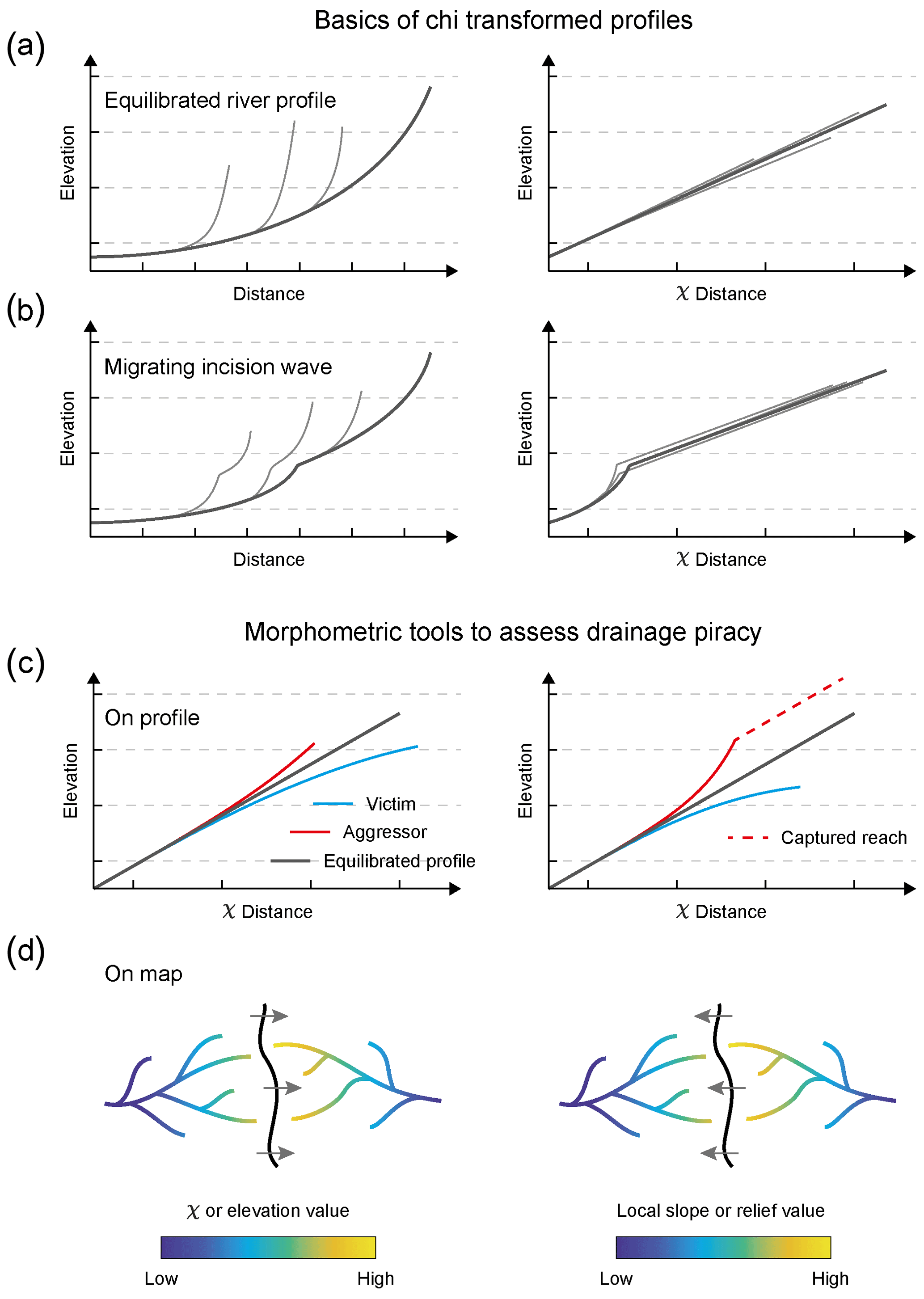
Figure 4Schematic river profiles and metrics expected in the case of equilibrated rivers, of a wave of incision migrating upstream the river network, or of stream piracy and divide migration. (a) Longitudinal (left) and χ (right) profiles of a main trunk river (dark line) and its tributaries (grey lines) in the case that these rivers are in equilibrium with external forcing conditions that are constant over the whole area. The χ profiles of these various rivers are here all linear (constant forcing conditions) and colinear (same forcing conditions), within a certain variability related to natural conditions (Perron and Royden, 2013). (b) Longitudinal (left) and χ (right) profiles of a main trunk river (dark line) and its tributaries (grey lines) in the case of the migration of a wave of incision through the river network. Knickpoints are present along the various streams at variable locations, but their χ profiles are all concordant, within the variability due to natural conditions (Perron and Royden, 2013). (c) χ profiles expected in the case of migrating divides (left) or river captures (right). Aggressor (or pirate) stream is represented in red, and the victim in blue. The dark line represents the profile expected for rivers equilibrated with external forcing. Area gain shifts the χ profiles of aggressor streams to lower χ values, above the equilibrium line. Conversely, area loss shifts the χ profiles of victim streams to higher χ values, below the equilibrium line. Here, χ profiles are discordant (Willett et al., 2014). (d) Assessment of divide migration and its direction from the across-divide contrast in χ (Willett et al., 2014) (left) or in Gilbert metrics such as local slope or relief (Whipple et al., 2017b; Forte and Whipple, 2018) (right).
3.2.3 Computation of transformed coordinates (χ)
The computation of χ-transformed river coordinates has proved useful for the understanding of landscape and drainage network dynamics (e.g., Perron and Royden, 2013; Willett et al., 2014; Yang et al., 2015; Whipple et al., 2017b). In this coordinate system, the elevation z at a given position along the riverbed x depends of the integral quantity χ following Eq. (1):
with
where xb locates the channel outlet; A(x) is the drainage area upstream of the position x along the channel; A0 is a reference scaling area; m and n are constant empirical parameters most often expressed as the ratio. This ratio can be related to the reference concavity index θref that describes how the river gradient evolves along the river profile. Such integral approach is based on the stream power equation of river incision (e.g., Howard, 1994; Whipple and Tucker, 1999). It provides a simple metric for pointing out and analyzing variable forcing conditions or the nature of transient signals within the river network, by comparing trunk streams and their tributaries in profiles corrected for their variable upstream drainage areas – and therefore their variable spatial scales – (Perron and Royden, 2013) (Fig. 4).
The χ plot of an equilibrated concave river system obeying the stream power equation, with uniform conditions, is a straight line along which both main trunk stream and tributaries collapse (Fig. 4a). Furthermore, by setting A0 to unity, the slope of the χ profile is equal to the channel steepness Ksn (Perron and Royden, 2013). This metric is linked to the uplift rate U and the erodibility coefficient K, by the following equation:
For U and K varying along the profile of the river, steeper (gentler) segments in χ profiles relate either to locally higher (lower) uplift rate or to lower (higher) erodibility. However, any assessment of these parameters from river profiles is not direct and straightforward as they depend on parameter n, which is not known a priori (e.g., Mudd et al., 2018). In the following, we assume that there is no significant variation in the erosion processes over the study region. Also, we do not consider a specific value for n and use θref = 0.5 (see Supplement, in which the effect of the chosen concavity index is tested for θref ranging between 0.3 and 0.7). Such assumptions allow for a relative comparison between the various parts of the drainage network over our study area.
3.2.4 Assessment of the drainage network dynamics
We use transformed χ profiles to detect and analyze perturbations within the river network. Knickpoints in longitudinal profiles of main trunk and tributaries that migrate upstream following a wave of incision in response to a common change in forcing or boundary conditions are expected to cluster and be concordant in transformed coordinates (Perron and Royden, 2013) (Fig. 4b). Conversely, migrating knickpoints of differing origins (e.g., local discrete river captures) will be discordant both in longitudinal and χ profiles. In the case of migrating knickpoints, whether concordant or discordant in χ coordinates, the river steepness around knickpoints is representative neither of the actual local uplift rate nor of the erodibility, but rather of the upstream migration of an incision wave. Spatially fixed knickpoints, as a response to local variations in uplift or erodibility, are expected to be also discordant in transformed coordinates.
Transformed χ plots are also useful to unravel drainage reorganization related to migrating divides and river captures (Willett et al., 2014). A river capture leads to a characteristic χ profile (Willett et al., 2014) (Fig. 4c). Indeed, an abrupt increase in drainage area due to a capture shifts the profile of the pirate stream to lower χ values, i.e., above a theoretical equilibrium profile. Conversely, area loss shifts the profile of the victim stream to higher χ values, i.e., below a theoretical equilibrium profile (Fig. 4c). χ profiles of rivers affected by captures are therefore expected to be discordant, transiently after the capture and before re-equilibrating to the new boundary conditions. This is also expected for migrating divides without discrete captures (Yang et al., 2015), unless the response of channels to drainage area changes is faster than that of divide migration (Whipple et al., 2017b). Such signatures of captures or area loss by piracy in transformed coordinates are defined relatively to an equilibrium river profile, specified theoretically or in the field from equilibrated trunk or major rivers.
It should be noticed that a certain degree of discordance in transformed χ profiles is acceptable given the variability of natural conditions, even in the case of equilibrated rivers or in the case of rivers responding to a common wave of incision (Fig. 4a and b). We choose not to define quantitatively what could be taken as an acceptable degree of discordance in river profiles as it implies to specify a threshold that is by essence arbitrary. This will not affect our results, and conclusions as major knickpoints in Bhutan are largely dispersed and discordant in χ, amplitude and altitude.
We also use maps of χ along the drainage network to detect potential migrating divides and to assess the direction of these migrations. A contrast in the value of χ across a divide results in its migration toward the stream with the highest χ (Willett et al., 2014) (Fig. 4d). Recent studies show, however, that the direction of divide migration interpreted from a χ analysis is not straightforward and can be biased by the assumed river base level (Whipple et al., 2017b; Forte and Whipple, 2018). Spatially variable tectonic or climatic conditions, as well as rock properties, may also maintain χ contrasts across stable divides. To overcome these limitations, we strengthen our analysis of across-divide contrasts by using “Gilbert metrics” associated with contrasts in elevation of the riverbed, in mean upstream local slope and in mean upstream local relief at a given drainage reference area (Whipple et al., 2017b; Forte and Whipple, 2018), taken here as 2 km2. Migration of the divide is expected to occur towards the stream with relative higher elevation and conversely with relative lower local slope or relief (Fig. 4d).
In addition, we infer divide motion by locating morphological indicators of regressive erosion like beheaded channels (or wind gaps), from Google Earth satellite imagery or field observations. These complementary methods enable a more careful assessment of divide migration direction and drainage network re-organization.

Figure 5Projected and transformed profiles of major and large rivers in Bhutan. Rivers are located on the maps of Fig. 1, color-coded and labeled. Major knickpoints are also pointed by triangles. Regions with altitudes above 3800 m (grey area) are not to be compared directly to the downstream sections as these may have a glacial imprint. Portions of the rivers north of physiographic transition T3 are reported by transparent segments. (P)A: (proto-)Amo Chhu; (P)W: (proto-)Wang Chhu; P: Puna Tsang Chhu; M: Mangde Chhu; (P)C: (proto-)Chamkhar Chhu; K: Kuri Chhu; D: Dangme Chhu. (a) Longitudinal profiles projected along a north–south axis, approximately perpendicular to active tectonic structures and to structural directions (Fig. 1a). Except for the Wang Chhu, all major knickpoints are located ca. 75–80 km north of the mountain front. (b) Transformed river profiles, following the formalism of Perron and Royden (2013). The Gangetic Plain is used as the base level for all these rivers. χ-transformed profiles are established with a concavity of 0.5 (see Fig. S1 in the Supplement for similar transformed profiles but using other concavity values). (c) Theoretical transformed river profiles of the proto-Wang Chhu, proto-Amo Chhu and proto-Chamkhar Chhu, compared to the transformed profiles of other large rivers. Profiles of proto-rivers are determined here by removing all the drainage area upstream of the major knickpoint. A large portion of these theoretical profiles remains relatively flat in transformed coordinates (for χ > ca. 3000 m) as the steepness of these rivers is low near their knickpoint (immediately upstream and downstream), over a limited real distance of a few kilometers at most.
Table 1Drainage areas of large Himalayan rivers in Bhutan, taken upstream of their outlet at the mountain front or upstream of a major confluence.
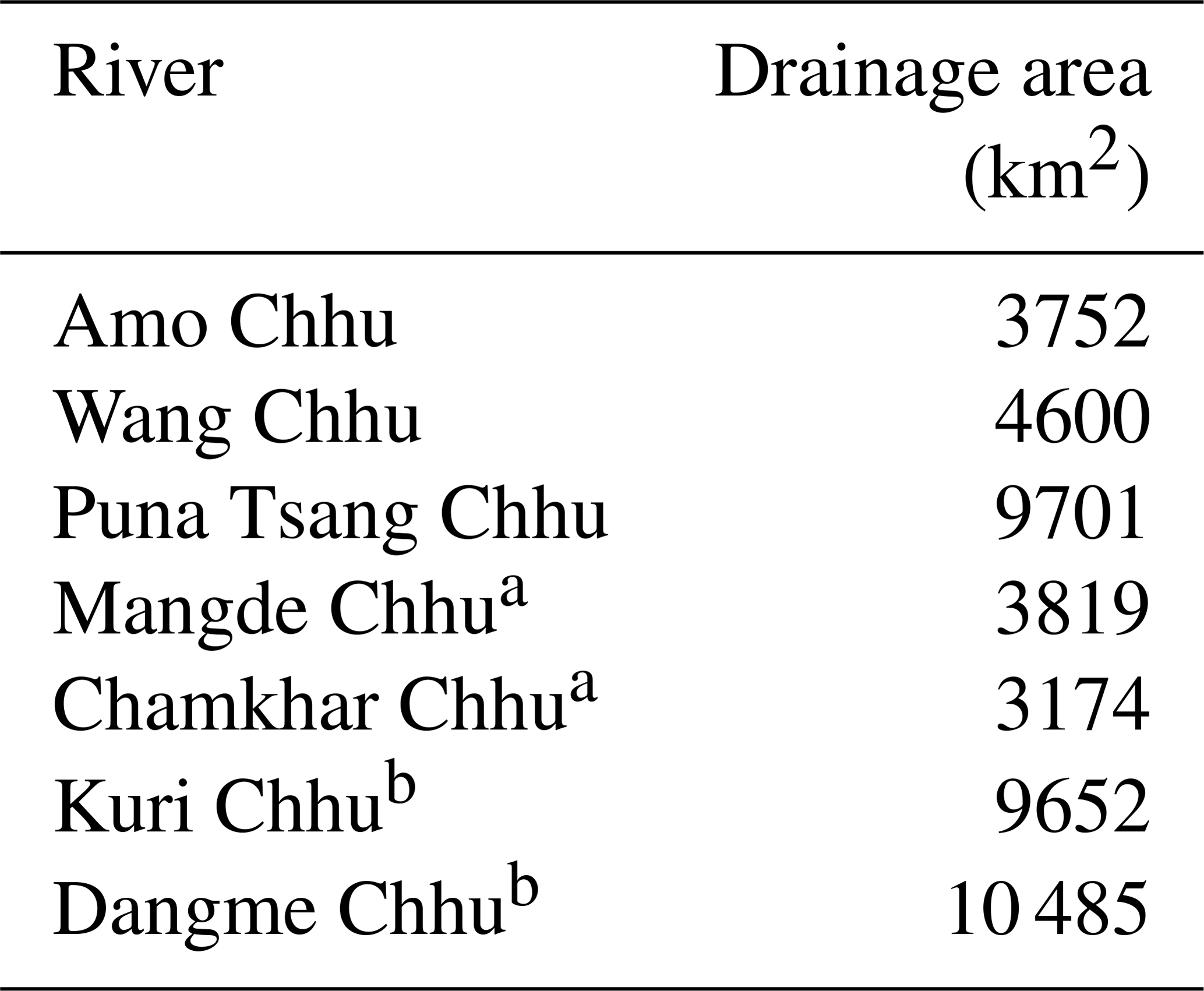
a The drainage areas of the Mangde Chhu and Chamkhar Chhu are here calculated upstream of their confluence. b The drainage areas of the Kuri Chhu and Dangme Chhu are here calculated upstream of their confluence.
4.1 General observations and definition of the spatial scales of investigation
Based on the visual interpretation of longitudinal and χ profiles, we define three profile types for major rivers in Bhutan (Figs. 2c and 5). First, the Kuri Chhu and Dangme Chhu in eastern Bhutan are characterized by concave upward profiles south of the High Himalayan range (south of physiographic transition T3), with no remarkable major knickpoint. These rivers correspond to the two largest drainage basins, with drainage areas > 9000 km2 (Table 1). Second, the Amo Chhu, Wang Chhu and Chamkhar Chhu have major knickpoints (> 1 km high), located approximately near T2. These knickpoints separate a steep river segment to the south from a river segment with lower gradient to the north. More specifically, the river portion with lower gradient flows within and across an alluvial plain (Fig. 3b) located in a high-altitude low-relief region (Fig. 1c). These rivers are those among the major Himalayan rivers of Bhutan with the smallest drainage basins (drainage areas of < 5000 km2) (Figs. 1 and S10 in the Supplement, Table 1). Third, the Puna Tsang Chhu and Mangde Chhu have intermediate characteristics: their longitudinal profile is overall concave upward with a more modest (< 1 km high) knickpoint near the region of T2, and they flow through a limited (Puna Tsang Chhu – Fig. 3a) or inexistent (Mangde Chhu) alluvial plain upstream of this knickpoint.
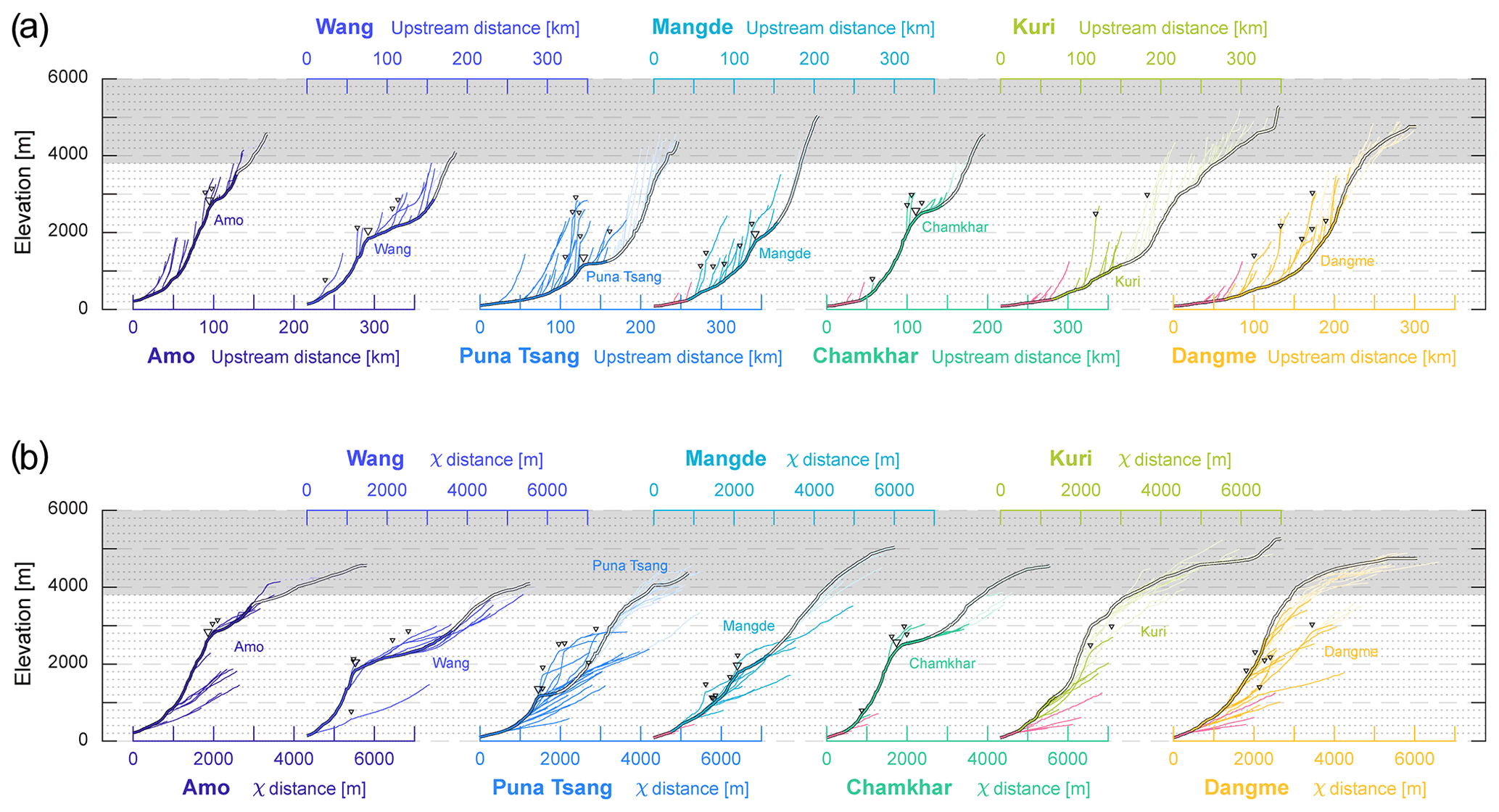
Figure 6Longitudinal (a – top) and transformed χ (b – bottom) profiles of major rivers of Bhutan and of their tributaries (with drainage area > 50 km2) (location in Fig. 1). Major drainage basins (and the corresponding horizontal axes of their profiles) are color-coded as in Fig. 1. Trunk streams are reported in bold lines and tributaries in thinner lines. Lighter transparent colors are used for the river portions north of physiographic transition T3. Major knickpoints are pointed out by triangles. Altitudes above 3800 m are considered aside (grey band) as rivers may preserve a glacial imprint in these regions. χ-transformed profiles are established with a concavity of 0.5. Other concavities have been tested and are illustrated in Fig. S2 in the Supplement. For an easier reading of the figure, horizontal axes (distance or χ) are alternatively reported below or above the graphs and follow the same color code as that of the rivers they are associated with.
These major rivers define the local base level for the incision of their tributaries (Fig. 6). Longitudinal profiles of tributaries exhibit a great variability relative to their trunk stream (Fig. 6a). This variability decreases and specific trends emerge when transformed into χ coordinates (Fig. 6b). On the one hand, most tributaries appear colinear with their trunk stream in χ plots – at least colinear in χ over comparable spatial regions of the mountain range, in particular at the level of their confluence. On the other hand, some tributaries plot above the trunk stream. These tributaries are characterized by a downstream steep channel and an upstream gentle segment. The gentle segments correspond to high-altitude low-relief patches of the landscape (Figs. 1 and 3c and d).
Given the above general observations of major rivers and of their tributaries, we define various scales of investigation of the landscape dynamics in Bhutan. First, we analyze major trunk rivers draining the Bhutan Himalaya and discuss their diversity. Next, we focus on those showing major knickpoints and flowing through alluvial plains in high-altitude low-relief regions of the range. We finally analyze the tributaries of main trunk rivers, in particular near perched low-relief regions. For each spatial scale, we describe our results and present the interpretations that can be directly derived from them. We recall that we focus hereafter only on the regions south of physiographic transition T3.
4.2 Major Himalayan rivers
Here, the longitudinal and χ profiles of the Kuri Chhu, Dangme Chhu, Puna Tsang Chhu and Mangde Chhu are discussed and compared (Figs. 2c and 5). Except for the Mangde Chhu, these rivers correspond to the largest drainage basins of Bhutan (Table 1).
The two easternmost major rivers (Kuri Chhu and Dangme Chhu) show a very similar long river profile, incising deep into the mountain range (Fig. 3f) as altitudes of ca. 2000 m are reached ca. 200 km from their outlet at the Gangetic Plain (Fig. 2c). This is also the case for the Puna Tsang Chhu, ca. 100–150 km further west in western Bhutan, which only departs locally from the previous longitudinal profiles by ca. 130 km from the outlet, at the level of its major – but relatively modest (ca. 300–400 m high) – knickpoint. The longitudinal profile of the Mangde Chhu is well above that of these other major rivers.
When transformed into χ coordinates, the profiles of these four rivers compare well and are overall colinear within our region of interest south of T3 (Fig. 5b). It should be emphasized here that the major knickpoints of the Puna Tsang Chhu and Mangde Chhu are not concordant in transformed coordinates, with variable χ and most importantly with altitudes that vary by ca. 600 m.
These observations suggest that major rivers share and have adjusted overall to similar tectonic and/or climatic forcing conditions in our region of interest, even though these rivers are located throughout Bhutan.
4.3 Large Himalayan rivers draining low-relief alluvial plains
The Chamkhar Chhu, Wang Chhu and Amo Chhu have longitudinal and χ profiles that are well above those of the formerly discussed major Bhutanese rivers (Figs. 2c and 5b). This is not surprising for longitudinal profiles as these three rivers have more modest drainage areas (Table 1), but this pattern remains even in χ coordinates. It should also be noticed that the profiles of these rivers are not colinear in χ coordinates, with χ values and altitudes of major knickpoints that vary by ca. 1000 and by ca. 1400 m, respectively (Fig. 5b).
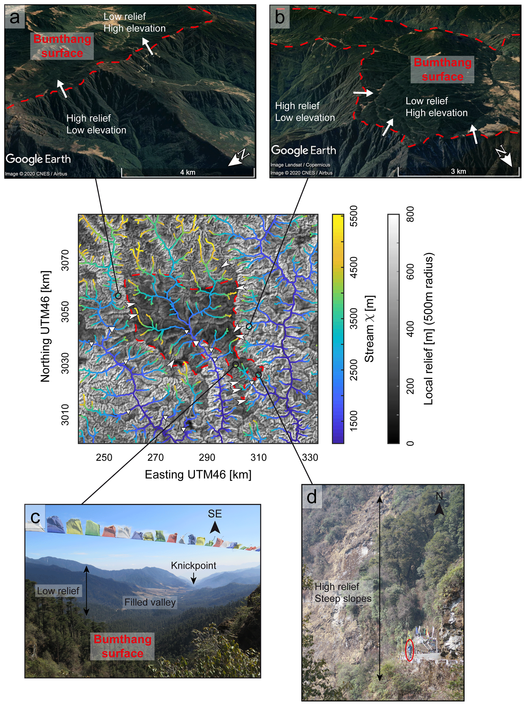
Figure 7Divide mobility around the high-altitude low-relief Bumthang region, from χ metrics, field and satellite observations. Central map (location on Fig. 1c) represents local relief, with a moving window of 500 m, and the identified low-relief region is delimited by the red dashed line. Major knickpoints are reported with inversed triangles, and arrows locate the existence of morphological observations of regressive erosion (wind gaps), together with the direction of the associated divide migration. χ values are reported along the river network as a criterion to assess divide mobility (following Willett et al., 2014) and are determined for a concavity of 0.5. Other metrics for the mobility of the drainage divides around the Bumthang region are reported in Fig. S3. Similar observations are reported for the Wang surface (Fig. S4). Satellite observations are taken from the Google Earth database. (a) © Google Earth view (image from CNES – Airbus 2020) of the relief and elevation contrasts across the western drainage divide of the Bumthang surface. White arrows locate observed beheaded channels (wind gaps) and indicate the direction of deduced drainage divide migration. (b) © Google Earth view (image from CNES – Airbus 2020 and Landsat – Copernicus) of the relief and elevation contrasts across the eastern drainage divide of the Bumthang surface. White arrows locate observed beheaded channels and indicate the direction of deduced drainage divide migration. (c) Field picture of the Sengor area (southeastern part of the Bumthang surface), where a filled valley is surrounded by higher relief rims. The filled valley is connected to the main river network by a tributary of the Kuri Chhu. A major knickpoint is present along this tributary, downstream of the pictured valley. Note the contrast in relief with picture (d), across the local delimitation of the Bumthang surface. (d) Field picture illustrating the extremely steep hillslopes along the western Kuri Chhu valley, immediately east of the Bumthang surface. A person is standing on the lower right side of the picture for scale (red circle). Note the contrast in relief with picture (c), across the local delimitation of the Bumthang surface.
These rivers are also characterized by the mobility of their drainage divides, as illustrated in Figs. 7 and S3 in the Supplement in the case of the Chamkhar Chhu. As intuitively expected, the high-altitude low-relief Bumthang region traversed by the Chamkhar Chhu is being laterally aggressed by the tributaries of the deeply incising Mangde Chhu (to the west) and Kuri Chhu (to the east). As a result, the main drainage divides around this low-relief region are migrating inwards, and the drainage area is locally shrinking (Figs. 7 and S3). The reverse situation is observed further south, downstream of the major knickpoint of the Chamkhar Chhu. Gilbert metrics suggest that drainage divides are here migrating outwards so that drainage area is locally increasing (Figs. 7 and S3). Similar observations and conclusions are reached for the Wang Chhu (Fig. S4), even though the situation of the Wang Chhu is slightly more complex.
Altogether, our results indicate that the Chamkhar Chhu and possibly the Wang Chhu, flowing through high-altitude low-relief alluvial plains in the hinterland, have overall disequilibrium characteristics. Their χ profiles, well above the regional average defined by the transformed profiles of other major rivers throughout Bhutan (Fig. 5b), are possibly indicative of a gain of drainage area by large-scale river captures (see Fig. 4c; following Willett et al., 2014; Yang et al., 2015). This interpretation is comforted by the fact that the transformed profiles of these rivers get closer to that of other major rivers when corrected for the drainage area upstream of their major knickpoints (proto-Amo Chhu, proto-Wang Chhu and proto-Chamkhar Chhu in Fig. 5c). Additionally, in the details, we find evidence for an ongoing dynamic rearrangement of the river network within these large drainage basins, with a specific pattern of drainage area loss and expansion on either side of their major knickpoint.
4.4 Low-relief regions captured by secondary streams
At a more local spatial scale, modest high-altitude low-relief regions (Fig. 3c and d) are connected to the main drainage network through secondary streams and tributaries, as for the Phobjikha and Yarab regions (Fig. 1c).
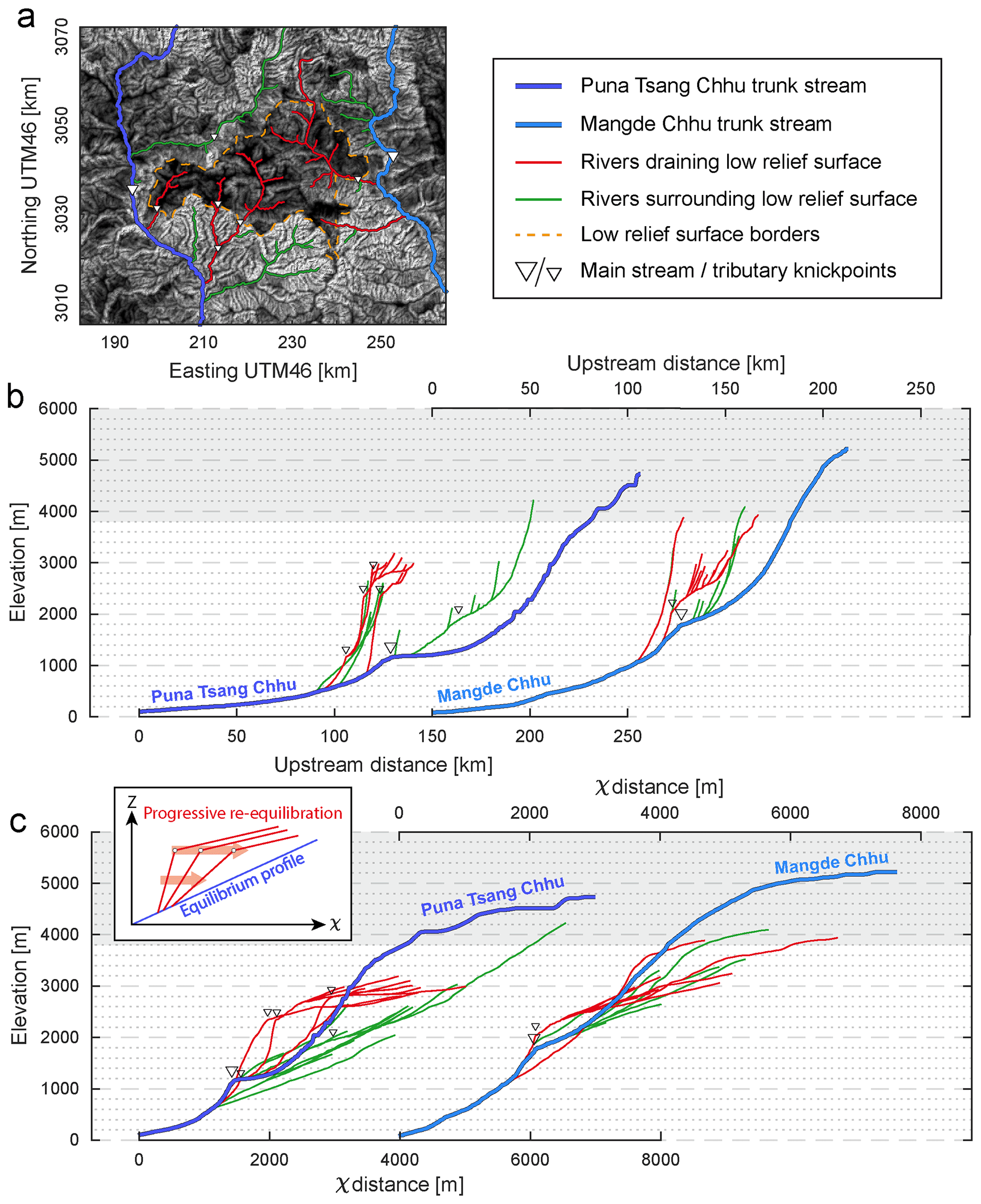
Figure 8Longitudinal and transformed river profiles around and within the Phobjikha high-altitude low-relief surface, following the approach of Yang et al. (2015). Comparable results are verified for the Yarab surface (Fig. S8 in the Supplement). (a) Map of topographic relief of the Phobjikha area (see Fig. 1c for location), with a moving window of 500 m (scale bar as in Fig. 9); the identified low-relief region is delimited by the orange dashed line. Major knickpoints are reported with inversed triangles. Tributaries of the Puna Tsang Chhu (west) and Mangde Chhu (east) trunk streams are color-coded, according to whether they drain the low-relief area (red) or are external to it (green). (b) Longitudinal river profiles of the Puna Tsang Chhu and Mangde Chhu, with main tributaries draining (red) or external (green) to the low-relief Phobjikha area. (c) Transformed river profiles of the same rivers. Tributaries draining the low-relief area (red) plot above the main trunk streams as is observed in the case of area gain by river capture (Fig. 4c). None of these profiles are concordant, indicating that these captures are not coeval and do not follow a coherent wave of incision propagating upstream. It should be noted that the higher the χ position of the knickpoints of the internal streams, the lower the steepness of the pirate streams downstream of their knickpoint. This is particularly illustrated by the Puna Tsang Chhu tributaries and is interpreted as reflecting progressive re-equilibration of pirate streams toward an equilibrium profile after capture (inset). Tributaries external to the low-relief area (green) are locally overall colinear with their main trunk stream, even though they gain drainage area by progressive divide migration (Fig. 9).
Starting from the profiles of Fig. 6, we further explore the main features of the drainage network within and around the Phobjikha surface using longitudinal and χ profiles of the secondary streams, with respect to their main trunk rivers, the Puna Tsang Chhu and Mangde Chhu (Fig. 8). We here follow the approach proposed by Yang et al. (2015) by differentiating streams draining the interior of this low-relief region and those flowing around. External streams (in green in Fig. 8) have χ profiles mostly colinear with their main trunk stream – and more specifically with the local χ profile of their trunk stream, near their confluence. In contrast, streams draining the Phobjikha low-relief surface (in red in Fig. 8) plot well above the Puna Tsang Chhu or Mangde Chhu in χ coordinates, with a high and low steepness downstream and upstream of a major knickpoint, respectively.
Interestingly, the streams draining the Phobjikha low-relief region have major knickpoints that are not concordant with the major knickpoint of their trunk stream in χ coordinates, with χ values and altitudes that vary by up to ca. 1500 and ca. 1600 m, respectively, in the case of the Puna Tsang Chhu and its tributaries (Fig. 8c). These streams show a peculiar pattern, most obvious in the case of the tributaries of the Puna Tsang Chhu: the greater the χ coordinate of the knickpoint, the lower the steepness of the stream segment downstream of the knickpoint, and therefore the closer (in χ coordinates) the stream profile gets to the regional average set by its trunk river (Fig. 8c).
None of the streams have χ profiles clearly below the regional average driven by their main trunk channels (Fig. 8c). It is also noteworthy that the χ profiles of the streams external to the Phobjikha surface (in green in Fig. 8) remain close to – and not above – the regional average imposed by their main trunk river (Fig. 8), even though they keep gaining drainage area by regressive erosion of the low-relief area. Indeed, across-divide contrasts in χ, relief and elevation suggest that the Phobjikha region is being regressively eroded all around by surrounding streams (Fig. 9), in particular along its western divide with the Puna Tsang Chhu as contrasts in χ (Fig. 9) and mostly elevation (Fig. S6 in the Supplement) are highest. Contrary to the previous observations on low-relief regions drained by the Wang Chhu and Chamkhar Chhu (Figs. 7, S3 and S4), there is no evidence here for a counteracting drainage area expansion of the streams draining this low-relief region downstream of it (Fig. 9). The area of this low-relief region is shrinking, and the streams draining it are losing drainage area.
Similar observations are obtained for the streams draining inside and outside the Yarab low-relief region, located in eastern Bhutan and surrounded by the Kuri Chhu and Dangme Chhu (see Figs. S7–S9 in the Supplement).
The characteristics of the streams draining elevated low-relief regions are interpreted as reflecting disequilibrium with drainage area gain by capture (Willett et al., 2014; Yang et al., 2015) (Fig. 4c). Our results (Figs. 8c, 9, and S5–S9) indicate that the discrete captures of low-relief regions have led to the punctual increase of drainage area of nearby pirate streams but have not impeded the ongoing continuous regressive erosion of these regions – therefore accompanied by area loss – along their divide with other surrounding aggressor streams. Discordant knickpoints suggest that these captures were discrete and non-coeval and that some of the pirate streams have had time to progressively partially re-equilibrate with their main trunk stream (inset in Fig. 8c). In contrast, the streams aggressing all around elevated low-relief regions are in overall equilibrium and keeping pace with the local incision set by their trunk streams, as indicated by their transformed profiles.
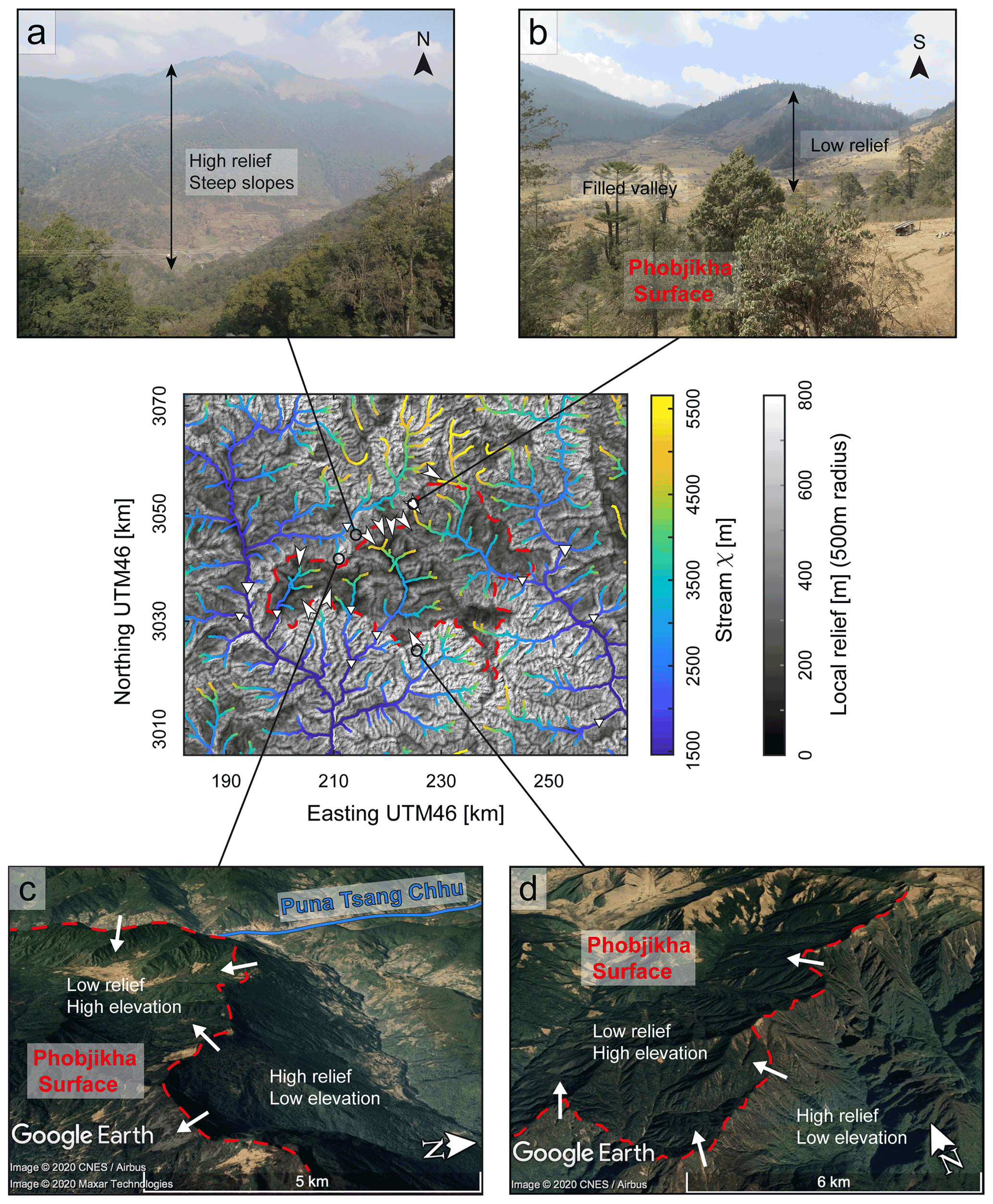
Figure 9Divide mobility around the high-altitude low-relief Phobjikha region, from χ metrics, field and satellite observations. Central map (location on Fig. 1c) represents local relief, with a moving window of 500 m, and the identified low-relief region is delimited by the red dashed line. Major knickpoints are reported with inversed triangles, and arrows locate the existence of morphological observations of regressive erosion (wind gaps), together with the direction of the associated divide migration. χ values are reported along the river network and are determined for a concavity of 0.5. Other complementary metrics of divide mobility are tested in Fig. S6. Similar observations are reported for the Yarab region (Fig. S7). Satellite observations are taken from the Google Earth database. (a) Field picture illustrating the high relief and steep slopes along the Dang Chhu (tributary of the Puna Tsang Chhu), along the northern boundary of the Phobjikha surface. Note the contrast in relief and slope with picture (b), across the local delimitation of the Phobjikha surface. (b) Field picture looking east of the Pele La pass (northern part of the Phobjikha surface), where a filled valley is surrounded by higher-relief rims. Note the contrast in relief with picture (a), across the local delimitation of the Phobjikha surface. (c) © Google Earth view (image from CNES – Airbus and Maxar Technologies 2020) of the relief and elevation contrasts across the northwestern drainage divide of the Phobjikha surface. White arrows locate observed beheaded channels (wind gaps) and indicate the direction of deduced drainage divide migration. (d) © Google Earth view (image from CNES – Airbus 2020) of the relief and elevation contrasts across the southern limit of the Phobjikha surface. White arrows locate observed beheaded channels and indicate the direction of deduced drainage divide migration.
4.5 Summary of key results
Altogether, we do not find in our results and field observations any evidence that the morphological characteristics of Bhutan were generated by a common wave of incision propagating upstream the drainage network. Indeed, all river profiles and their knickpoints are discordant in χ-transformed coordinates (Figs. 5c, 6b and 8c – by comparison to Fig. 4b), whatever the spatial scale of investigation. This finding is supported by the secondary drainage network of rivers flowing through or around high-altitude low-relief regions since all these streams share a common base level and their χ profiles can be more rigorously compared (Fig. 8c). The documented χ profiles of major or secondary rivers support the existence of ubiquitous discrete and non-coeval river captures of low-relief regions in Bhutan.
Our results also suggest that a steady-state morphology is far from being reached in the Bhutan Himalaya. Only few major rivers (the Kuri Chhu and Dangme Chhu, and to some extent the Puna Tsang Chhu and Mangde Chhu) have profiles associated with a potential equilibrium with tectonic and climatic forcing throughout the mountain range. The other large Himalayan rivers (Chamkhar Chhu and Wang Chhu) keep a record of large-scale captures and show peculiar dynamics on either side of their major knickpoint, with apparent drainage area loss and expansion upstream and downstream of the knickpoint, respectively (Fig. 7). This dynamic response of rivers is more pronounced at smaller spatial scales, where some secondary streams have captured high-altitude low-relief regions and where others are progressively gaining drainage area by the regressive erosion of these same regions (Figs. 8 and 9).
5.1 Limits on our analysis and results
5.1.1 Limits related to possible lateral variations in tectonics or climate
The comparison between the various Himalayan rivers throughout Bhutan may be limited by possible lateral variations in boundary and forcing conditions. The widespread occurrence of Greater Himalayan series (Fig. 1a) limits large-scale lithological variations. Tethyan or Lesser Himalayan series are also present in central and eastern Bhutan. However, spatial variations in bedrock erodibility associated with these variations are expected to be limited (Lavé and Avouac, 2001; Adams et al., 2020).
Climate is tropical and wet everywhere. Precipitation varies mostly along a latitudinal transect across the range, with extreme precipitation rates of over 6 m yr−1 along the mountain front (Baillie and Norbu, 2004; Bookhagen and Burbank, 2006; Grujic et al., 2006). Within our region of interest in the mountain hinterland, present-day precipitation rates are relatively moderate everywhere, with values of ca. 1–2 m yr−1. Longitudinal variations from east to west related to the rain shadow formed by the Shillong Plateau in the foreland are minor. As large rivers are mostly flowing north–south, perpendicular to the main climatic trend, they are all similarly affected and the cross-comparison of river profiles as done here is permitted.
The Amo Chhu and Wang Chhu are the two rivers of westernmost Bhutan where significant lateral structural and tectonic variations may be expected, as they are located in the vicinity of the Paro structural window and of the Yadong graben (e.g., Gansser, 1983; Long et al., 2011a; Greenwood et al., 2016) (Fig. 1a). Similarly, a structural window into Lesser Himalayan series prevails along the Kuri Chhu (Fig. 1a), where variations in the seismic coupling of the MHT have been recently evidenced (Marechal et al., 2016), suggesting other possible lateral variations in tectonics further east. In western and eastern Bhutan, we therefore cannot exclude the possibility of a tectonic forcing different from that encountered in central Bhutan.
It should be noticed that the profiles and characteristics of the Wang Chhu and Amo Chhu in western Bhutan are overall comparable to those of the Chamkhar Chhu in central Bhutan. Additionally, the Yarab high-altitude low-relief surface in eastern Bhutan shares common attributes with the Phobjikha low-relief patch in central western Bhutan. In general, most geomorphic features specific to the Bhutan Himalaya are found along a longitudinal band throughout this whole region of the Himalayas (Fig. 1c). Together these observations suggest that the lateral variations in tectonics, climate or lithology documented in Bhutan may have only a minor effect on the observed morphology.
5.1.2 Limits related to the morphometric approach
The comparison of river profiles in χ-transformed coordinates requires a common base level for all streams. Tributaries with a common trunk stream meet this specific condition, but the comparison of major rivers with different and independent outlets is not straightforward. To overcome this limitation, we assume that the base level of all major rivers is the Gangetic Plain, which has an almost constant elevation of ca. 100–120 m south of the mountain front. For this reason, the absence of evidence for a coherent wave of incision is mostly evidenced from the joint analysis of tributaries and of their trunk stream (Fig. 8c) and only suggested by the comparison of major rivers (Fig. 5b).
A coherent wave of incision migrating upstream the drainage network may not be straightforward to elucidate in transformed χ profiles in the case of an unstable drainage network, where divide migration and captures prevail throughout the landscape. This has been illustrated in field cases where the dispersion of knickpoints (in transformed coordinates) associated with the upstream migration of a wave of incision is interpreted to relate to the coeval changes in upstream drainage area due to divide migration (Schwanghart and Scherler, 2020) or river captures (Giachetta and Willett, 2018). In the case of the Bhutan Himalaya, river captures leave a clear and significant imprint on the river network (Figs. 5b and 8c) and may hide the signature of other processes. As further discussed hereafter (see Sect. 5.2), the river network appears to adjust much faster to progressive changes in drainage area due to the mobility of divides, so that the affected streams keep adjusting to the incisional pace of their trunk river or to changes of main river base level. This results in the fact that divide migration does not leave a specific signature on the transformed profiles of these rivers (Fig. 8c), which would have permitted here for keeping the record of an incision wave if existent.
χ analyses are based on the stream power concept and do not include the effect of sediments on river incision (Gasparini et al., 2007). This can limit our interpretations for rivers with alluvial plains or for secondary streams capturing low-relief regions. It has been shown that discordant χ profiles could be achieved for rivers enduring a common wave of incision when incision is dependent on the sediment flux (Giachetta and Willett, 2018). In this case, a positive correlation between drainage area and upstream knickpoint migration is expected as drainage area supposedly approximates available sediment fluxes (Giachetta and Willett, 2018), which we have not clearly found in our data (Fig. S8).
When calculating χ values and transformed river profiles, drainage area is taken as a proxy for river discharge (Eq. 1) (e.g., Perron and Royden, 2013). This implies that precipitation rates are supposedly constant over the considered drainage basin, an assumption not verified here (Bookhagen and Burbank, 2006; Grujic et al., 2006) as in most large-scale watersheds. Spatial variations in rainfall have been shown to alter river profiles (Han et al., 2014, 2015). Here, locally higher than average precipitation rates lead to locally higher river discharges and may be mistaken for a false gain in drainage area. This should not, however, alter and impact our results and interpretations. First, extreme precipitation rates are only found along the mountain front in Bhutan, by ca. 50 km north of physiographic transition T1 at most, and therefore south of our region of interest where major knickpoints (Fig. 5a) and high-altitude low-relief regions (Fig. 2a and b) are found. Lastly, our interpretations rely on the cross-comparison of river profiles that are all expected to be similarly affected as all large rivers flow across the main north–south climatic trend.
Some of our inferences are therefore dependent on the known limitations of χ analyses and of the stream power approach in general. However, these should not affect our main conclusions on river captures or migrating divides – and therefore on the unstable and dynamic pattern of the river network – as they are based on the cross-comparison of rivers affected by overall similar latitudinal tectonic and climatic forcing, and are further corroborated by field and satellite observations, as well as by across-divide contrasts in Gilbert metrics (Figs. 7, 9, S3, S4, S6 and S7).
5.2 River captures, migrating divides and timescales of landscape response
Secondary streams external to low-relief areas progressively gain drainage area by regressive erosion (Figs. 7 and 9). Transformed profiles of these tributaries remain close to the regional trend of trunk channels (Fig. 8c). This observation suggests that the channel response is here faster than that of the perturbation driven by divide migration, consistent with conclusions from recent numerical experiments by Whipple et al. (2017b). This result implies that drainage re-organization by progressive divide migration is not expected to leave a particular geomorphic signature, most probably because of a relatively high erosional efficiency (Whipple et al., 2017b), in contrast with other field cases where the time for divide migration may have outpaced that of the erosional river response (Schwanghart and Scherler, 2020).
Only drainage area increase by discrete stream capture appears to leave a significant imprint on the river network. Our results suggest that river captures have occurred at all spatial scales in the hinterland of Bhutan, from large-scale captures in the case of the Wang Chhu or Chamkhar Chhu, with high (> 1 km) major knickpoints (Fig. 5b), to more modest captures in the case of the secondary streams draining high-altitude low-relief regions (Fig. 8). Discordant profiles and the observed variable position of knickpoints in χ coordinates and altitude favor the idea that these captures are discrete and not coeval in time and that pirate streams have been progressively returning to equilibrium (Fig. 8c). These captures result in a large and abrupt drainage area increase, which requires a subsequent longer time for the rivers to adapt to their new boundary conditions. Such particular conditions are discussed by Whipple et al. (2017b) using the relative ratio of the timescale of channel response to a characteristic recurrence time of large capture events. Following this reasoning, our results suggest that river captures leave an imprint on river profiles if captures occur more often than the time needed to adjust to their new conditions, or if the last capture event is younger than the timescale for channel response. These various considerations imply that only the most recent landscape evolution can be retrieved from morphometric approaches, leaving little – if no – possibility to access the morphologic conditions prior to the most recent captures.
5.3 Geomorphological characteristics of the Bhutan Himalaya
Our results were previously presented following the various spatial scales of investigation. Below, we provide a synthesis of our observations for each geomorphic feature whatever associated spatial scale and discuss possible explanations of their origin. We finally compare our findings and inferences to previous interpretations.
5.3.1 Major knickpoints within the river network
Knickpoints along large Himalayan rivers of Bhutan separate two domains, with drainage area expansion downstream of the knickpoint and drainage area reduction upstream (Figs. 7, S3 and S4). Such dynamics on either side of a knickpoint have already been observed in other contexts of major river captures, such as for the Douro river in Spain and Portugal (Struth et al., 2019). The tool effect of sediments remobilized from the upstream-captured alluvial plain may favor incision downstream of the knickpoint, which would propagate laterally towards the divides and lead locally to the outward expansion of drainage area. Such consequent drainage area gain may additionally boost river incision and the lowering of the local base level. These positive feedbacks are expected to favor and enhance the upstream migration of the major knickpoint (e.g., Giachetta and Willett, 2018; Struth et al., 2019). However, an additional – but negative – feedback may operate as the drainage area reduction upstream of the knickpoint may limit and refrain the upstream knickpoint migration (Schwanghart and Scherler, 2020). Such feedback, by eventually significantly lowering the expected upstream migration of major knickpoints, may contribute to the preservation and surface uplift of the upstream low-relief region over time, to the over-steepening of the downstream river segments and therefore to the large dimensions of observed major knickpoints. If the reduction in the rate of knickpoint migration by upstream drainage area loss were significant, knickpoints along major Bhutanese rivers could appear as more or less stationary.
Major knickpoints are observed at all scales (Fig. 6). They follow a specific spatial organization as most of them are localized in the Bhutan hinterland, near physiographic transition T2, regardless of the size of the associated drainage basin (Figs. 1b and c and 5a). This co-location looks surprising in the case of non-coeval discrete stream captures at various spatial scales. It may therefore suggest that knickpoint migration remains limited in space, near T2. This indicates that these knickpoints originated and have possibly been maintained locally.
5.3.2 High-altitude low-relief regions
Transformed profiles of the rivers draining elevated low-relief regions all show a specific pattern indicative of river captures, regardless of their spatial scale (Figs. 5b and 8c). Discordant χ profiles at all scales (Figs. 5b, 6b and 8c) suggest that these captures were not coeval. Conversely, no evidence for a counteracting drainage area loss by stream piracy appears in χ profiles of nearby rivers, as none of the profiles are below the regional equilibrium line delineated by the profiles of large Himalayan rivers (Fig. 5b) or of trunk streams in the case of secondary low-relief regions (Fig. 8c). It has been noticed that area loss by piracy is not as well expressed in transformed coordinates as is area gain by capture (see Fig. 9b of Whipple et al., 2017b). Because the absence of χ river profiles below estimated regional averages is observable at all spatial scales, even when large-scale captures are suspected, it could be postulated that such captures have not been at the expense of other rivers, but of the low-relief regions themselves if once isolated from the drainage network. Even though not common, internally drained basins exist in tropical contexts. The Sun Moon Lake region of central Taiwan is an example, where internally drained basins are on the verge of being captured (Toushe Basin), or where similar captures are suspected (Yushi and Puli Basins) (see discussion by Simoes et al., 2014). Because the timescale for river response to changes in boundary conditions is expected to be relatively short in Bhutan (see Sect. 5.2), the conditions that lead to the relief lowering and isolation of the landscape patches investigated here, prior to their capture, may not have left a clear morphologic record.

Figure 10Topography and relief along the hinterland of the Bhutan Himalaya, where low-relief surfaces are located. WS: Wang surface; PS: Phobjikha surface; BS: Bumthang surface; YS: Yarab surface. (a) Topographic map of the Bhutan Himalaya from ALOS World 3D – 30 m (AW3D30) DEM data. Main drainage basins are delineated by black lines, and associated main rivers are color-coded (color code as in Fig. 1). The dashed rectangle locates the swath profile represented in (b). (b) Topographic swath profile along the Bhutan hinterland, with elevations taken within the band illustrated in Fig. 10a. Location of major rivers and of low-relief regions are reported. (c) Map of local relief, as calculated from the topography shown in Fig. 10a, with a moving window of 500 m. Major high-altitude low relief areas are delineated by dashed red lines. Main rivers are located and color-coded. The dashed rectangle locates the swath profile represented in (d) and encompasses the same region as that of Fig. 10a. (d) Swath profile of relief along the Bhutan hinterland, with relief taken within the band located in Fig. 10c. Low-relief regions of the mountain range interior are reported. The lower-relief values of the swath profile are to be considered for low-relief regions.
Swath profiles across the Bhutan hinterland illustrate that elevated low-relief regions have overall similar altitudes and local relief (Fig. 10), regardless of their spatial scale, as if resulting from the surface uplift and subsequent dissection of the same initial topographic surface (after Whipple et al., 2017a). However, morphometric analyses may mostly detect the lowest-relief patches, as these offer the highest relief contrast with other regions (Fig. 1c). We cannot therefore discard the possibility that other low-relief patches (but with relatively higher relief) exist at other altitudes, as suspected for instance to the east and north-east of the Yarab region (Fig. S8). In the case that relief reduction is concomitant to surface uplift, such as when low-relief regions are formed by area loss during drainage re-organization (Whipple et al., 2017a), local relief is expected to correlate with altitude. The similar altitude and local relief of low-relief regions (Fig. 10) may therefore either favor the idea of local remnants of relict landscapes or be indicative of the in situ formation of these regions during uplift.
The limits of these regions most often coincide with drainage divides (“coincident divides” in the sense of Willett, 2017) with numerous beheaded channels, in particular for secondary regions (Figs. 7 and 9). This observation, together with that of local low denudation rates (Adams et al., 2016) and relief (Figs. 7 and 9), of alluvial filling (Fig. 3d and e) and well-developed soils (Fig. 3b–d) (Baillie et al., 2004; Adams et al., 2016) in valleys surrounded by higher-relief rims (Figs. 3b and d, 7 and 9), favors the idea that these low-relief regions were formed in situ while uplifted, before their capture (Willett, 2017). Area loss related to the dynamic re-organization of the drainage network (after Willett et al., 2014; Yang et al., 2015) could be a plausible mechanism given the ample evidence for captures and divide mobility. A local rise in base level, as in the case of defeated uplifted hanging valleys, is another possibility, as described in other contexts (e.g., Burbank et al., 1996; Fernandez-Blanco et al., 2020).
These possible interpretations only describe the type of morphological response of the river network leading to the formation of these features (relief lowering and isolation of these regions) but do not provide the processes driving this response. We emphasize that the high-altitude low-relief regions are all co-located in the hinterland of Bhutan, in between physiographic transitions T2 and T3, whatever their spatial scales and dimensions (Fig. 1c). This strongly suggests that they were most probably formed only locally and not pervasively throughout Bhutan, appealing for a local process driving and supporting their formation, preservation and subsequent dissection.
5.3.3 The spatial organization of all major knickpoints and low-relief regions calls for a common local tectonic origin
Our investigations illustrate the highly dynamic – and eventually unstable – pattern of the river network in the Bhutan hinterland. Despite these dynamics, both major knickpoints and high-altitude low-relief regions, whatever their spatial scale, all are co-located in the hinterland of the Bhutan Himalaya, along an approximately west–east-oriented spatial band near physiographic transition T2 or in between T2 and T3 (Fig. 1b and c). This observation calls for a common local genetic origin for all these features and for the observed network dynamics. This holds throughout most of the Himalayas of Bhutan, even in eastern Bhutan, where no major knickpoint exists along the Kuri Chhu and Dangme Chhu at these latitudes (Figs. 1 and 5). The presence of the Yarab low-relief region, localized in between these two major rivers (Fig. 1c), indicates that a similar mechanism is also ongoing in this part of the Himalayan range (Figs. S7–S9). The absence of a major knickpoint on adjacent large rivers reveals that these have sufficient power to adjust to local conditions. The only minor exception to the observed colocation is the major knickpoint of the Wang Chhu in western Bhutan, which is deported ca. 20–30 km southward from the observed longitudinal band (Figs. 1 and 5a).
This spatial geomorphological organization is not expected to be controlled lithologically as it is clearly not correlated to surface geology (Fig. 1a). Alternatively, the orientation of the swath containing all major knickpoints and low-relief regions supports the idea of a local tectonic driver in the mountain hinterland, as this orientation is parallel to major active tectonic structures (such as the frontal MFT or MBT – Fig. 1a) or associated geomorphic expressions (such as the High Himalayan range expectedly above a mid-crustal ramp of the MHT) (Figs. 1b and 2).
Additionally, the east–west swath encompassing the investigated geomorphic peculiarities of the Bhutan Himalaya also approximately follows the orientation of the precipitation pattern in Bhutan and is slightly north of the band of highest precipitation rates (e.g., Bookhagen and Burbank, 2006; Grujic et al., 2006). Such a climatic pattern results from the major orographic barrier formed by the steeply rising topography between physiographic transitions T1 and T2 (Fig. 2a and b), for which tectonics are the most probable driver. As such, we propose that the peculiar geomorphic dynamics, the steep topography between T1 and T2, and the associated local climatic pattern all share an initial common tectonic driver. The observed and investigated landscape characteristics is therefore interpreted to first reflect active tectonics in the hinterland of Bhutan, but the interplay between local uplift, the associated high slopes and climate may modulate and enhance local landscape dynamics (e.g., Adams et al., 2020).
5.3.4 Discussing previous interpretations in light of our findings
The absence of evidence for a coherent wave of incision moving upstream the drainage network (Figs. 5b, 6b and 8c) and the spatial organization of observed geomorphic features only along a longitudinal band (Fig. 1) exclude previous interpretations relying on any large-scale change in tectonics or climate over Bhutan. This is the case for the model of tectonic rejuvenation of Bhutan relative to the Himalaya of central Nepal (Duncan et al., 2003) or for that of a general surface uplift of Bhutan consequent to decreasing precipitation in the rain shadow of the rising Shillong Plateau (Grujic et al., 2006). The dimensions of the major knickpoints of some of the large rivers, with heights of > 1 km in the cases of the Amo Chhu, Wang Chhu or Chamkhar Chhu (Figs. 2c and 5), are most probably too large to be related to a wave of incision migrating upstream into a relict landscape, as a response to a change in relative base level.
Baillie and Norbu (2004) proposed that the variety of river profiles were related to lateral variations in tectonic uplift throughout Bhutan. This may potentially explain part of the discordance in χ profiles of major and large rivers (Fig. 5b). In this case the spatial co-location of knickpoints throughout Bhutan, within a west–east swath (Figs. 1 and 5a), would indicate that the location of active tectonics is coherent along strike but that only the rates of active deformation are laterally variable. Even though lateral variations in the rates of uplift cannot be excluded, these are not expected to vary significantly, and in particular randomly from one valley to the other. Additionally, the similar steepness of large rivers south of T2, located variably in western (Puna Tsang Chhu), central (Mangde Chhu) and eastern (Kuri Chhu and Dangme Chhu) Bhutan (Fig. 5b), calls for overall similar rates of uplift, given the similar lithologic (Fig. 1a) and climatic (e.g., Bookhagen and Burbank, 2006; Grujic et al., 2006) conditions. This interpretation is supported by the fact that the theoretical steepnesses of the proto-Wang Chhu and proto-Chamkhar Chhu, prior to their suspected large-scale captures, are similar to those of these other large rivers, south of T2 (Fig. 5c). Also, the presence of the high-altitude low-relief Yarab surface in eastern Bhutan indicates that similar first-order conditions prevail in this part of the Himalaya even though the two major surrounding rivers (the Kuri Chhu and Dangme Chhu) have no major knickpoint. Similar tectonics, in terms of patterns and also in terms of rates, are therefore expected throughout Bhutan despite the variability of fluvial profiles. In fact, this variability is rather expected to relate to the various responses and capacities of the different rivers to adjust to local tectonics (Fig. S10) and to the existence or not of recent captures.
Adams et al. (2016) proposed that major knickpoints and low-relief regions were the geomorphic response to recent uplift over a blind duplex in the Bhutan hinterland. Interestingly coming at it from another angle, their interpretation meets our deductions that the observed geomorphic features need to be primarily sustained locally by ongoing active uplift. The proposed tectonic perturbation originates in the hinterland and not at the base level of major rivers, which may account to some extent for discordant χ profiles (Fig. 5b). Our results therefore confirm their primary conclusion on the need for active tectonics in the hinterland and additionally document some aspects of the landscape dynamics that were not explored.
To move a step forward, some details of the Adams et al. (2016) model could be refined in light of our findings. Major knickpoints were interpreted by these authors as setting the local base level for the in situ filling of upstream uplifted valleys. In their model, knickpoints migrate upstream and upwards, and while doing so remove fill deposits. If this were the case, upstream knickpoint migration (from the tectonic perturbation) would be expected to correlate with knickpoint altitude, upstream drainage area and the extent of uplifted alluvial fill, which is not specifically observed (Fig. S10). Indeed, the co-location of all major knickpoints whatever considered spatial scale, from major to local rivers (Fig. 1), indicates that these knickpoints are relatively stationary (see Sect. 5.3.1). Our deductions agree with the conclusions of Adams et al. (2016) that high-altitude low-relief regions were formed in situ while uplifted. We find, however, evidence that these regions may have been defeated and isolated once from the main network before being captured (see Sect. 5.3.2), which contrasts with the continuously through-flowing and adjusting uplifted rivers supported by Adams et al. (2016). Such differences in the details of the origin and evolution of the low-relief regions become important when it comes to derive surface uplift from a theoretical (poorly resolved) initial river profile by comparison to the present-day profiles. One possible future research direction aiming at better understanding the dynamics of major knickpoints and the formation and evolution of low-relief regions in Bhutan would be to model the landscape evolution in response to local uplift in the mountain hinterland, following the initial work of Adams et al. (2016) but adding the dynamic response of the river network through migrating divides and river captures. Finally, denudation rates should be considered with great caution when used as proxies for uplift rates in places where the shape of drainage basins is far from being stable, as is the case here (e.g., Sassolas-Serrayet et al., 2019). It should be also emphasized that uplift rates are expected to vary across strike, with higher rates over the blind ramp and with lower rates downstream and upstream of it, further challenging the comparison between denudation rates measured in high-relief canyons and those in upstream alluvial or isolated low-relief valleys.
Based on field observations and on a quantitative and qualitative morphometric analysis of the mountain hinterland in Bhutan at various spatial scales, we have further documented the landscape dynamics of this part of the Himalayas where out-of-equilibrium morphologies have been described. We find that the various geomorphic features of the Bhutanese landscape, such as major knickpoints or high-altitude low-relief regions, are most probably not related to the migration of a wave of incision upstream the river network. Rather, our analysis emphasizes the existence of numerous drainage captures, at various spatial scales, spatially discrete and temporally non-coeval, with partial re-equilibrations of captured drainages in some cases. In addition to these captures, drainage divides are found to migrate in various parts of the hinterland, in particular around or downstream elevated low-relief regions, with efficient re-equilibration of river profiles as expected in the case of relatively fast landscape response.
Our results therefore emphasize the existence of an unstable and dynamic landscape, which however obeys a specific spatial organization along a longitudinal spatial band in the mountain range interior. This latter key observation supports the idea that the documented geomorphic dynamics need to be sustained locally by tectonic uplift. Even though the idea proposed by Adams et al. (2016) of uplift over a blind ramp in the hinterland is consistent with our conclusions, some of their deductions do not capture or account for the observed high dynamics of the river network. This is most probably because they base their deductions on the comparison to a landscape evolution simulation in which drainage divides remain stationary. Future work exploring the initial idea of Adams et al. (2016) of active tectonic uplift in the mountain hinterland but with account on the possible dynamic response of the river network is therefore needed.
Finally, because the drainage network is not stable with ubiquitous divide migrations in the hinterland, the previous use of denudation rates as a proxy for tectonic uplift rates in Bhutan (Le Roux-Mallouf et al., 2015; Adams et al., 2016) may be problematic, and results should be re-evaluated. Our work therefore emphasizes the need for a precise investigation of landscape dynamics and disequilibrium over various spatial scales as a first essential step in morpho-tectonic studies of active landscapes.
This study relies on topographic data obtained from the ALOS World 3D – 30 m (AW3D30) digital elevation model (DEM) provided by the Japanese Aerospace Exploration Agency, accessible at: https://www.eorc.jaxa.jp/ALOS/en/aw3d30/index.htm (last access: July 2021) (ALOS, 2021). The MATLAB-based function library TopoToolbox used in this study for morphometric analyses is accessible at: https://topotoolbox.wordpress.com (last access: July 2021) (TopoToolbox, 2021). Satellite images were taken from the Google Earth database.
The supplement related to this article is available online at: https://doi.org/10.5194/esurf-9-895-2021-supplement.
MS designed and conceptualized the research objectives of this study. She also wrote the main draft of the manuscript with contributions from all co-authors. TSS carried the presented geomorphic analyses and prepared all associated figures. RC gathered all the necessary financial support that led to the work presented here. All co-authors participated in fieldwork, scientific discussions and the co-editing of the manuscript.
The authors declare that they have no conflict of interest.
Publisher's note: Copernicus Publications remains neutral with regard to jurisdictional claims in published maps and institutional affiliations.
This article benefitted from constructive comments by Wolfgang Schwanghart and an anonymous reviewer, and Associated Editor Sébastien Castelltort is thanked for the handling of the manuscript. The fruitful discussions that led to this article arose during fieldwork in Bhutan, and our friend and driver, Phajo Kinley (Department of Geology and Mines, Thimphu), is warmly thanked for taking good care of us all during our various journeys. Through the work of Martine Simoes, this study stands as IPGP contribution no. 4223.
This study benefitted from grants from the Agence National de la Recherche (France) attributed to RC, through projects ANR BhutaNepal (ANR grant no. ANR-13-BS06-0006) and TopoExtreme (ANR grant no. ANR-18-CE01-0017). Timothée Sassolas-Serrayet benefitted from a PhD grant attributed by the French Ministry of Higher Education and Research. Through the work of Martine Simoes, this study contributes to the IdEx Université de Paris ANR-18-IDEX-0001.
This paper was edited by Sebastien Castelltort and reviewed by Wolfgang Schwanghart and one anonymous referee.
Adams, B. A., Hodges, K. V., van Soest, M. C., and Whipple, K. X.: Evidence for Pliocene–Quaternary normal faulting in the hinterland of the Bhutan Himalaya, Lithosphere, 5, 438–449, 2013.
Adams, B. A., Hodges, K. V., Whipple, K. X., Ehlers, T. A., van Soest, M. C., and Wartho, J.-A.: Constraints on the tectonic and landscape evolution of the Bhutan Himalaya from thermochronometry, Tectonics, 34, 1329–1347, https://doi.org/10.1002/2015TC003853, 2015.
Adams, B. A., Whipple, K. X., Hodges, K. V., and Heimsath, A. M.: In situ development of high-elevation, low-relief landscapes via duplex deformation in the Eastern Himalayan hinterland, Bhutan, J. Geophys. Res., 121, 294–319, https://doi.org/10.1002/2015JF003508, 2016.
Adams, B. A., Whipple, K. X., Forte, A. M., Heimsath, A. M., and Hodges, K. V.: Climate controls on erosion in tectonically active landscapes, Science Advances, 6, eaaz3166, https://doi.org/10.1126/sciadv.aaz3166, 2020.
Adlakha, V., Lang, K. A., Patel, R. C., Lal, N., and Huntington, K. W.: Rapid long-term erosion in the rain shadow of the Shillong Plateau, Eastern Himalaya, Tectonophysics, 582, 76–83, https://doi.org/10.1016/j.tecto.2012.09.022, 2013.
Allen, P. A.: From landscapes into geological history, Nature, 451, 274–276, https://doi.org/10.1038/nature06586, 2008.
ALOS: ALOS Global Digital Surface Model “ALOS World 3D – 30 m (AW3D30)”, available at: https://www.eorc.jaxa.jp/ALOS/en/aw3d30/index.htm, last access: July 2021.
Babault, J., Bonnet, S., Van Den Driessche, J., and Crave, A.: High elevation of low-relief surfaces in mountain belts: does it equate to post-orogenic surface uplift?, Terra Nova, 19, 272–277, https://doi.org/10.1111/j.1365-3121.2007.00746.x, 2007.
Babault, J., Van Den Driessche, J., and Teixell, A.: Longitudinal to transverse drainage network evolution in the High Atlas (Morocco): The role of tectonics, Tectonics, 31, TC4020, https://doi.org/10.1029/2011TC003015, 2012.
Baillie, I. C. and Norbu, C.: Climate and other factors in the development of river and interfluve profiles in Bhutan, Eastern Himalayas, J. Asian Earth Sci., 22, 539–553, 2004.
Baillie, I. C., Tshering, K., Dorji, T., Tamang, H. B., Dorji, T., Norbu, C., Hutcheon, A. A., and Baumler, R.: Regolith and soils in Bhutan, Eastern Himalayas, Eur. J. Soil Sci., 55, 9–27, https://doi.org/10.1046/j.1365-2389.2003.00579.x, 2004.
Beaumont, C., Jamieson, R. A., Nguyen, M. H., and Lee, B.: Himalayan tectonics explained by extrusion of a low-viscosity crustal channel coupled to focused surface denudation, Nature, 414, 738–742, https://doi.org/10.1038/414738a, 2001.
Beeson, H. W., McCoy, S. W., and Keen-Zebert, A.: Geometric disequilibrium of river basins produces long-lived transient landscapes, Earth Planet. Sc. Lett., 475, 34–43, https://doi.org/10.1016/j.epsl.2017.07.010, 2017.
Berthet, T., Ritz, J.-F., Ferry, M., Pelgay, P., Cattin, R., Drukpa, D., Braucher, R., and Hetenyi, G.: Active tectonic of the eastern Himalaya: new constraints from the first tectonic geomorphology study in southern Bhutan, Geology, 42, 427–430, 2014.
Bilham, R.: Himalayan earthquakes: a review of historical seismicity and early 21st century slip potential, Geological Society, London, Special Publications, 483, 423–482, https://doi.org/10.1144/SP483.16, 2019.
Biswas, S., Coutand, I., Grujic, D., Hager, C., Stockli, D., and Grasemann, B.: Exhumation and uplift of the Shillong Plateau and its influence on the eastern Himalayas: New constraints from apatite and zircon (U-Th-[Sm])/He and apatite fission track analyses, Tectonics, 26, TC6013, https://doi.org/10.1029/2007TC002125, 2007.
Bollinger, L., Avouac, J. P., Beyssac, O., Catlos, E. J., Harrison, T. M., Grove, M., Goffé, B., and Sapkota, S.: Thermal structure and exhumation history of the Lesser Himalaya in central Nepal, Tectonics, 23, TC5015, https://doi.org/10.1029/2003TC001564, 2004.
Bollinger, L., Henry, P., and Avouac, J. P.: Mountain building in the Nepal Himalaya: Thermal and kinematic model, Earth Planet. Sc. Lett., 244, 58–71, https://doi.org/10.1016/j.epsl.2006.01.045, 2006.
Bonnet, S. and Crave, A.: Landscape response to climate change: Insights from experimental modeling and implications for tectonic versus climatic uplift of topography, Geology, 31, 123–126, 2003.
Bookhagen, B. and Burbank, D. W.: Topography, relief, and TRMM-derived rainfall variations along the Himalaya, Geophys. Res. Lett., 33, L08405, https://doi.org/10.1029/2006GL026037, 2006.
Burbank, D. W., Meigs, A., and Brozovic, N.: Interactions of growing folds and coeval depositional systems, Basin Res., 8, 199–223, https://doi.org/10.1046/j.1365-2117.1996.00181.x, 1996.
Burbank, D. W., Blythe, A. E., Putkonen, J., Pratt-Sitaula, B., Gabet, E., Oskin, M., Barros, A., and Ojha, T. P.: Decoupling of erosion and precipitation in the Himalayas, Nature, 426, 652–655, https://doi.org/10.1038/nature02187, 2003.
Castelltort, S., Goren, L., Willett, S. D., Champagnac, J.-D., Herman, F., and Braun, J.: River drainage patterns in the New Zealand Alps primarily controlled by plate tectonic strain, Nat. Geosci., 5, 744–748, https://doi.org/10.1038/NGEO1582, 2012.
Cattin, R. and Avouac, J. P.: Modeling mountain building and the seismic cycle in the Himalaya of Nepal, J. Geophys. Res., 105, 13389–13407, 2000.
Clark, M. K. and Bilham, R.: Miocene rise of the Shillong Plateau and the beginning of the end for the Eastern Himalaya., Earth Planet. Sc. Lett., 269, 337–351, https://doi.org/10.1016/j.epsl.2008.01.045., 2008.
Clift, P. D., Giosan, L., Carter, A., Garzanti, E., Galy, V., Tabrez, A. R., Pringle, M., Campbell, I. H., France-Lanord, C., Blusztan, J., Allen, C., Alizai, A., Luckge, A., Danish, M., and Rabbani, M. M.: Monsoon control over erosion patterns in the Western Himalaya: possible feed-back into the tectonic evolution, Geological Society, London, Special Publications, 342, 185–218, https://doi.org/10.1144/SP342.12, 2010.
Coutand, I., Whipp, D. M. J., Grujic, D., Bernet, M., Fellin, M. G., Bookhagen, B., Landry, K. R., Ghalley, S. K., and Duncan, C.: Geometry and kinematics of the Main Himalayan Thrust and Neogene crustal exhumation in the Bhutanese Himalaya derived from inversion of multithermochronologic data, J. Geophys. Res., 119, 1446–1481, https://doi.org/10.1002/2013JB010891, 2014.
Coutand, I., Barrier, L., Govin, G., Grujic, D., Hoorn, C., Dupont-Nivet, G., and Najman, Y.: Late Miocene-Pleistocene evolution of India-Eurasia convergence partitioning between the Bhutan Himalaya and the Shillong Plateau: New evidences from foreland basin deposits along the Dungsam Chu section, eastern Bhutan, Tectonics, 35, 2963–2994, https://doi.org/10.1002/2016TC004258, 2016.
DeCelles, P. G., Robinson, D. M., Quade, J., Ojha, T. P., Garzione, C. N., Copeland, P., and Upreti, B. N.: Stratigraphy, structure, and tectonic evolution of the Himalayan fold-and-thrust belt in western Nepal, Tectonics, 20, 487–509, 2001.
Diehl, T., Singer, J., Hetenyi, G., Grujic, D., Clinton, J., Giardini, D., Kissling, E., and group, G. W.: Seismotectonics of Bhutan: Evidence for segmentation of the Eastern Himalayas and link to foreland deformation, Earth Planet. Sc. Lett., 471, 54–64, https://doi.org/10.1016/j.epsl.2017.04.038, 2017.
Drukpa, D., Velasco, A. A., and Doser, D. I.: Seismicity in the Kingdom of Bhutan (1937–2003): Evidence for crustal transcurrent deformation, J. Geophys. Res., 111, B06301, https://doi.org/10.1029/2004JB003087, 2006.
Duncan, C., Masek, J., and Fielding, E.: How steep are the Himalaya ? Characteristics and implications of along-strike topographic variations, Geology, 31, 75–78, 2003.
Fernandez-Blanco, D., de Gelder, G., Lacassin, R., and Armijo, R.: Geometry of Flexural Uplift by Continental Rifting in Corinth, Greece, Tectonics, 39, e2019TC005685, https://doi.org/10.1029/2019TC005685, 2020.
Forte, A. M. and Whipple, K. X.: Criteria and Tools for Determining Drainage Divide Stability, Earth Planet. Sc. Lett., 493, 102–117, https://doi.org/10.1016/j.epsl.2018.04.026, 2018.
Gansser, A.: Geology of the Himalayas, Wiley-Interscience, New York, USA, 1964.
Gansser, A.: Geology of the Bhutan Himalaya, Birkhauser Verlag, Basel, Switzerland, 1983.
Gasparini, N. M., Whipple, K. X., and Bras, R. L.: Predictions of steady state and transient landscape morphology using sediment-flux-dependent river incision models, J. Geophys. Res., 112, F03S09, https://doi.org/10.1029/2006JF000567, 2007.
Gautam, P. and Rösler, W.: Depositional chronology and fabric of Siwalik group sediments in Central Nepal from magnetostratigraphy and magnetic anisotropy, J. Geophys. Res., 17, 659–682, 1999.
Giachetta, E. and Willett, S. D.: Effects of river capture and sediment flux on the evolution of plateaus: indights from numerical modeling and river profile analysis in the Upper Blue Nile catchment, J. Geophys. Res., 123, 1187–1217, https://doi.org/10.1029/2017JF004252, 2018.
Godard, V., Cattin, R., and Lavé, J.: Numerical modeling of mountain building: Interplay between erosion law and crustal rheology, Geophys. Res. Lett., 31, L23607, https://doi.org/10.1029/2004GL021006, 2004.
Godard, V., Bourlès, D. L., Spinabella, F., Burbank, D. W., Bookhagen, B., Fischer, G. B., Moulin, A., and Léanni, L.: Dominance of tectonics over climate in Himalayan denudation, Geology, 42, 243–246, https://doi.org/10.1130/G35342.1, 2014.
Goren, L., Willett, S. D., Herman, F., and Braun, J.: Coupled numerical–analytical approach to landscape evolution modeling, Earth Surf. Proc. Land., 39, 522–545, https://doi.org/10.1002/esp.3514, 2014.
Govin, G., Najman, Y., Copley, A., Millar, I., van der Beek, P., Huyghe, P., Grujic, D., and Davenport, J.: Timing and mechanism of the rise of the Shillong Plateau in the Himalayan foreland, Geology, 46, 279–282, https://doi.org/10.1130/G39864.1, 2018.
Greenwood, L. V., Argles, T. W., Parrish, R. R., Harris, N. B. W., and Warren, C.: The geology and tectonics of central Bhutan, J. Geol. Soc. London, 173, 352–369, https://doi.org/10.1144/jgs2015-031, 2016.
Grujic, D., Coutand, I., Bookhagen, B., Bonnet, S., Blythe, A., and Duncan, C.: Climatic forcing of erosion, landscape, and tectonics in the Bhutan Himalayas, Geology, 34, 801–804, https://doi.org/10.1130/G22648.1, 2006.
Guerit, L., Goren, L., Dominguez, S., Malavieille, J., and Castelltort, S.: Landscape 'stress' and reorganization from chi-maps: Insights from experimental drainage networks in oblique collision setting, Earth Surf. Proc. Land., 43, 3152–3163, https://doi.org/10.1002/esp.4477, 2018.
Guillot, S. and Le Fort, P.: Geochemical constraints on the bimodal origin of High Himalayan leucogranites, Lithos 35, 221–234, https://doi.org/10.1016/0024-4937(94)00052-4, 1995.
Hammer, P., Berthet, T., Hetenyi, G., Cattin, R., Drukpa, D., Chophel, J., Lechmann, S., Le Moigne, N., Champollion, C., and Doerflinger, E.: Flexure of the India plate underneath the Bhutan Himalaya, Geophys. Res. Lett., 40, 4225–4230, https://doi.org/10.1002/grl.50793, 2013.
Han, J., Gasparini, N. M., Johnson, J. P. L., and Murphy, B. P.: Modeling the influence of rainfall gradients on discharge, bedrock erodibility, and river profile evolution, with application to the Big Island, Hawai'i, J. Geophys. Res.-Earth, 119, 1418–1440, https://doi.org/10.1002/2013JF002961, 2014.
Han, J., Gasparini, N. M., and Johnson, J. P. L.: Measuring the imprint of orographic rainfall gradients on the morphology of steady-state numerical fluvial landscapes, Earth Surf. Proc. Land., 40, 1334–1350, https://doi.org/10.1002/esp.3723, 2015.
Hasbargen, L. E. and Paola, C.: Landscape instability in an experimental drainage basin, Geology, 28, 1067–1070, 2000.
Hetenyi, G., Le Roux-Mallouf, R., Berthet, T., Cattin, R., Cauzzi, C., Phunthso, K., and Grolimund, R.: Joint approach combining damage and paleoseismol- ogy observations constrains the 1714 AD Bhutan earthquake at magnitude 8 ± 0.5, Geophys. Res. Lett., 43, 10695–10702, https://doi.org/10.1002/2016GL071033, 2016.
Hirschmiller, J., Grujic, D., Bookhagen, B., Coutand, I., Huyghe, P., Mugnier, J. L., and Ojha, T. P.: What controls the growth of the Himalayan foreland fold-and-thrust belt?, Geology, 42, 247–250, https://doi.org/10.1130/G35057.1, 2014.
Hodges, K. V., Wobus, C. W., Ruhl, K., Schildgen, T., and Whipple, K. X.: Quaternary deformation, river steepening, and heavy precipitation at the front of the Higher Himalayan ranges, Earth Planet. Sc. Lett., 220, 379–389, https://doi.org/10.1016/S0012-821X(04)00063-9, 2004.
Howard, A. D.: A detachment-limited model of drainage basin evolution, Water Resour. Res., 30, 2261–2285, https://doi.org/10.1029/94WR00757, 1994.
Hubbard, J., Almeida, R., Foster, A., Sapkota, S. N., Burgi, P., and Tapponnier, P.: Structural segmentation controlled the 2015 Mw 7.8 Gorkha earthquake rupture in Nepal, Geology, 44, 639–642, https://doi.org/10.1130/G38077.1, 2016.
Huygue, P., Galy, A., Mugnier, J. L., and France-Lanord, C.: Propagation of the thrust system and erosion in the Lesser Himalaya: Geochemical and sedimentological evidence, Geology, 29, 1007–1010, 2001.
Iwata, S., Narama, C., and Karma: Three Holocene and late Pleistocene glacial stages inferred from moraines in the Lingshi and Thanza village areas, Bhutan, Quatern. Int., 97–98, 69–78, https://doi.org/10.1016/s1040-6182(02)00052-6, 2002.
Lavé, J. and Avouac, J. P.: Fluvial incision and tectonic uplift across the Himalayas of central Nepal, J. Geophys. Res., 106, 26561–26591, 2001.
Le Fort, P., Cuney, M., Deniel, C., France-Lanord, C., Sheppard, S. M. F., Upreti, B. N., and Vidal, P.: Crustal generation of the Himalayan leucogranites, Tectonophysics, 134, 39–57, 1987.
Le Roux-Mallouf, R., Godard, V., Cattin, R., Ferry, M., Gyeltshen, J., Ritz, J.-F., Drukpa, D., Guillou, V., Arnold, M., Aumaître, G., Bourlès, D. L., and Keddadouche, K.: Evidence for a wide and gently dipping Main Himalayan Thrust in western Bhutan, Geophys. Res. Lett., 42, 3257–3265, https://doi.org/10.1002/2015GL063767, 2015.
Le Roux-Mallouf, R., Ferry, M., Ritz, J.-F., Berthet, T., Cattin, R., and Drukpa, D.: First paleoseismic evidence for great surface-rupturing earthquakes in the Bhutan Himalayas, J. Geophys. Res., 121, 7271–7283, https://doi.org/10.1002/2015JB012733, 2016.
Le Roux-Mallouf, R., Ferry, M., Cattin, R., Ritz, J.-F., Drukpa, D., and Pelgay, P.: A 2600-year-long paleoseismic record for the Himalayan Main Frontal Thrust (western Bhutan), Solid Earth, 11, 2359–2375, https://doi.org/10.5194/se-11-2359-2020, 2020.
Liu, G. and Einsele, G. J. G. R.: Sedimentary history of the Tethyan basin in the Tibetan Himalayas, Geol. Rundsch., 83, 32–61, 1994.
Long, S., McQuarrie, N., Tobgay, T., Grujic, D., and Hollister, L.: Geologic Map of Bhutan, J. Maps, 7, 184–192, https://doi.org/10.4113/jom.2011.1159, 2011a.
Long, S., McQuarrie, N., Tobgay, T., Rose, C., Gehrels, G., and Grujic, D.: Tectonostratigraphy of the Lesser Himalaya of Bhutan: Implications for the along-strike stratigraphic continuity of the northern Indian margin, Geol. Soc. Am. Bull., 123, 1406–1426, https://doi.org/10.1130/B30202.1, 2011b.
Long, S. P., Mcquarrie, N., Tobgay, T., Coutand, I., Cooper, F. J., Reiners, P. W., Wartho, J.-A., and Hodges, K. V.: Variable shortening rates in the eastern Himalayan thrust belt, Bhutan: Insights from multiple thermochronologic and geochronologic data sets tied to kinematic reconstructions, Tectonics, 31, TC5004, https://doi.org/10.1029/2012TC003155, 2012.
Lyon-Caen, H. and Molnar, P.: Constraints on the structure of the Himalaya from an analysis of gravity anomalies and a flexural model of the lithosphere, J. Geophys. Res., 88, 8171–8191, https://doi.org/10.1029/JB088iB10p08171, 1983.
Lyon-Caen, H. and Molnar, P.: Gravity anomalies, flexure of the Indian Plate, and the structure, support and evolution of the Himalaya and Ganga Basin, Tectonics, 4, 513–538, https://doi.org/10.1029/TC004i006p00513, 1985.
Marechal, A., Mazzotti, S., Cattin, R., Cazes, G., Vernant, P., Drukpa, D., Thinley, K., Tarayoun, A., Le Roux-Mallouf, R., Thapa, B. B., Pelgay, P., Gyeltshen, J., Doerflinger, E., and Gautier, S.: Evidence of interseismic coupling variations along the Bhutan Himalayan arc from new GPS data, Geophys. Res. Lett., 43, 12399–12406, https://doi.org/10.1002/2016GL071163, 2016.
Matmon, A., Bierman, P. R., Larsen, J., Southworth, S., Pavich, M., and Caffee, M.: Temporally and spatially uniform rates of erosion in the southern Appalachian Great Smoky Mountains, Geology, 31, 155–158, https://doi.org/10.1130/0091-7613(2003)031<0155:TASURO>2.0.CO;2, 2003.
McQuarrie, N., Robinson, D., Long, S., Tobgay, T., Grujic, D., Gehrels, G., and Ducea, M.: Preliminary stratigraphic and structural architecture of Bhutan: Implications for the along strike architecture of the Himalayan system, Earth Planet. Sc. Lett., 272, 105–117, https://doi.org/10.1016/j.epsl.2008.04.030, 2008.
Meyer, M. C., Hofmann, C. C., Gemmell, A. M. D., Haslinger, E., Hausler, H., and Wangda, D.: Holocene glacier fluctuations and migration of Neolithic yak pastoralists into the high valleys of northwest Bhutan, Quaternary Sci. Rev., 28, 1217–1237, https://doi.org/10.1016/j.quascirev.2008.12.025, 2009.
Mudd, S. M., Clubb, F. J., Gailleton, B., and Hurst, M. D.: How concave are river channels?, Earth Surf. Dynam., 6, 505–523, https://doi.org/10.5194/esurf-6-505-2018, 2018.
Perron, J. T. and Royden, L.: An integral approach to bedrock river profile analysis, Earth Surf. Proc. Land., 38, 570–576, https://doi.org/10.1002/esp.3302, 2013.
Prince, P. S., Spotila, J. A., and Henika, W. S.: Stream capture as driver of transient landscape evolution in a tectonically quiescent setting, Geology, 39, 823–826, https://doi.org/10.1130/G32008.1, 2011.
Robinson, D. M., DeCelles, P. G., Patchett, P. J., and Garzione, C. N.: The kinematic evolution of the Nepalese Himalaya interpreted from Nd isotope, Earth Planet. Sc. Lett., 192, 507–521, 2001.
Rosenkranz, R., Schildgen, T., Wittmann, H., and Spiegel, C.: Coupling erosion and topographic development in the rainiest place on Earth: Reconstructing the Shillong Plateau uplift history with in-situ cosmogenic 10Be, Earth Planet. Sc. Lett., 483, 39–51, https://doi.org/10.1016/j.epsl.2017.11.047, 2018.
Sassolas-Serrayet, T., Cattin, R., Ferry, M., Godard, V., and Simoes, M.: Estimating the disequilibrium in denudation rates due to divide migration at the scale of river basins, Earth Surf. Dynam., 7, 1041–1057, https://doi.org/10.5194/esurf-7-1041-2019, 2019.
Schelling, D. and Arita, K.: Thrust tectonics, crustal shortening, and the structure of the far-eastern Nepal Himalaya, Tectonics, 10, 851–862, 1991.
Schwanghart, W. and Scherler, D.: Short Communication: TopoToolbox 2 – MATLAB-based software for topographic analysis and modeling in Earth surface sciences, Earth Surf. Dynam., 2, 1–7, https://doi.org/10.5194/esurf-2-1-2014, 2014.
Schwanghart, W. and Scherler, D.: Bumps in river profiles: uncertainty assessment and smoothing using quantile regression techniques, Earth Surf. Dynam., 5, 821–839, https://doi.org/10.5194/esurf-5-821-2017, 2017.
Schwanghart, W. and Scherler, D.: Divide mobility controls knickpoint migration on the Roan Plateau (Colorado, USA), Geology, 48, 698–702, https://doi.org/10.1130/G47054.1, 2020.
Simoes, M., Braun, J., and Bonnet, S.: Continental-scale erosion and transport laws: A new approach to quantitatively investigate macroscale landscapes and associated sediment fluxes over the geological past, Geochem. Geophy. Geosy., 11, Q09001, https://doi.org/10.1029/2010GC003121, 2010.
Simoes, M., Chen, Y.-G., Shinde, D. P., and Singhvi, A. K.: Lateral variations in the long-term slip rate of the Chelungpu fault, Central Taiwan, from the analysis of deformed fluvial terraces, J. Geophys. Res., 119, 3740–3766, https://doi.org/10.1002/2013JB010057, 2014.
Singer, J., Kissling, E., Diehl, T., and Hetenyi, G.: The underthrusting Indian crust and its role in collision dynamics of the Eastern Himalaya in Bhutan: Insights from receiver function imaging, J. Geophys. Res., 122, 1152–1178, https://doi.org/10.1002/2016JB013337, 2017.
Stevens, V. and Avouac, J. P.: Interseismic coupling on the Main Himalayan Thrust., Geophys. Res. Lett., 42, 5828–5837, https://doi.org/10.1002/2015GL064845, 2015.
Struth, L., Garcia-Castellanos, D., Viaplana-Muzas, M., and Verges, J.: Drainage network dynamics and knickpoint evolution in the Ebro and Duero basins: from endorheism to exorheism, Geomorphology, 327, 554–571, https://doi.org/10.1016/j.geomorph.2018.11.033, 2019.
Thiede, R. C., Bookhagen, B., Arrowsmith, J. R., Sobel, E. R., and Strecker, M. R.: Climatic control on rapid exhumation along the Southern Himalayan Front, Earth Planet. Sc. Lett., 222, 791–806, https://doi.org/10.1016/j.epsl.2004.03.015, 2004.
Thiede, R. C., Arrowsmith, J. R., Bookhagen, B., McWilliams, M. O., Sobel, E. R., and Strecker, M. R.: From tectonically to erosionally controlled development of the Himalayan orogen, Geology, 33, 689–692, https://doi.org/10.1130/G21483AR.1, 2005.
Tobgay, T., Mcquarrie, N., Long, S., Kohn, M. J., and Corrie, S. L.: The age and rate of displacement along the Main Central Thrust in the western Bhutan Himalaya, Earth Planet. Sc. Lett., 319–320, 146–158, 2012.
TopoToolbox: Mean basin ksn and smoothing madness, available at: https://topotoolbox.wordpress.com, last access: July 2021.
Tucker, G. E., Lancaster, S. T., Gasparini, N. M., Bras, R. L., and Rybarczyk, S. M.: An object-oriented framework for distributed hydrologic and geomorphic modeling using triangulated irregular networks, Computer & Geosciences, 27, 959–973, https://doi.org/10.1016/s0098-3004(00)00134-5, 2001.
Upreti, B. N.: An overview of the stratigraphy and tectonics of the Nepal Himalaya, J. Asian Earth Sci., 17, 577–606, 1999.
Verma, R. and Mukhopadhyay, M.: An analysis of the gravity field in northeastern India, Tectonophysics, 42, 283–317, 1977.
Viaplana-Muzas, M., Babault, J., Dominguez, S., Van Den Driessche, J., and Legrand, X.: Drainage network evolution and patterns of sedimentation in an experimental wedge, Tectonophysics, 664, 109–124, https://doi.org/10.1016/j.tecto.2015.09.007, 2015.
Viaplana-Muzas, M., Babault, J., Dominguez, S., Van Den Driessche, J., and Legrand, X.: Modelling of drainage dynamics influence on sediment routing system in a fold-and-thrust belt, Basin Res., 31, 290–310, https://doi.org/10.1111/bre.12321, 2019.
Whipple, K. X. and Meade, B. J.: Controls on the strength of coupling among climate, erosion, and deformation in two-sided, frictional orogenic wedges at steady state, J. Geophys. Res., 109, F01011, https://doi.org/10.1029/2003JF000019, 2004.
Whipple, K. X. and Meade, B. J.: Orogen response to changes in climatic and tectonic forcing, Earth Planet. Sc. Lett., 243, 218–228, https://doi.org/10.1016/j.epsl.2005.12.022, 2006.
Whipple, K. X. and Tucker, G. E.: Dynamics of the stream-power river incision model: implications for height limits of mountain ranges, landscape response timescales, and research needs, J. Geophys. Res., 104, 17661–17674, https://doi.org/10.1029/1999JB900120, 1999.
Whipple, K. X., DiBiase, R. A., Ouimet, W. B., and Forte, A. M.: Preservation or piracy: diagnosing low-relief, high-elevation surface formation mechanisms – Reply, Geology, 45, e422, https://doi.org/10.1130/G39252Y.1, 2017a.
Whipple, K. X., Forte, A. M., DiBiase, R. A., Gasparini, N. M., and Ouimet, W. B.: Timescales of landscape response to divide migration and drainage capture: Implications for the role of divide mobility in landscape evolution, J. Geophys. Res., 122, 248–273, 2017b.
Willett, S. D.: Preservation or piracy: diagnosing low-relief, high-elevation surface formation mechanisms – Comment, Geology, 45, e421, https://doi.org/10.1130/G38929C.1, 2017.
Willett, S. D. and Brandon, M. T.: On steady states of mountain belts, Geology, 30, 175–178, 2002.
Willett, S. D., Slingerland, R., and Hovius, N.: Uplift, shortening, and steady state topography in active mountain belts, Am. J. Sci., 301, 455–485, 2001.
Willett, S. D., McCoy, S. W., Perron, J. T., Goren, L., and Chen, C. Y.: Dynamic reorganization of river basins, Science, 343, 1248765, https://doi.org/10.1126/science.1248765, 2014.
Yang, R., Willett, S. D., and Goren, L.: In situ low-relief landscape formation as a result of river network disruption, Nature, 520, 526–529, https://doi.org/10.1038/nature14354, 2015.
Yin, A., Dubey, C., Webb, A., Kelty, T., Grove, M., Gehrels, G., and Burgess, W.: Geologic correlation of the Himalayan orogen and Indian craton: Part 1. Structural geology, U-Pb zircon geochronology, and tectonic evolution of the Shillong Plateau and its neighboring regions in NE India, Geol. Soc. Am. Bull., 122, 336–359, 2010.