Transmissivity and groundwater flow exert a strong influence on drainage density

The extent to which groundwater flow affects drainage density and erosion has long been debated but is still uncertain. Here, I present a new hybrid analytical and numerical model that simulates groundwater flow, overland flow, hillslope erosion and stream incision. The model is used to explore the relation between groundwater flow and the incision and persistence of streams for a set of parameters that represent average humid climate conditions. The results show that transmissivity and groundwater flow exert a strong control on drainage density. High transmissivity results in low drainage density and high incision rates (and vice versa), with drainage density varying roughly linearly with transmissivity. The model evolves by a process that is defined here as groundwater capture, whereby streams with a higher rate of incision draw the water table below neighbouring streams, which subsequently run dry and stop incising. This process is less efficient in models with low transmissivity due to the association between low transmissivity and high water table gradients. A comparison of different parameters shows that drainage density is most sensitive to transmissivity, followed by parameters that govern the initial slope and base level. The results agree with field data that show a negative correlation between transmissivity and drainage density. These results imply that permeability and transmissivity exert a strong control on drainage density, stream incision and landscape evolution. Thus, models of landscape evolution may need to explicitly include groundwater flow.

1 Introduction

Drainage density is a fundamental property of the Earth's surface that controls erosion and the transport of water and sediments. Drainage density has been observed to vary with climate, vegetation, relief, and soil and rock properties (Tucker et al., 2001b; Luo et al., 2016). Several analytical models have been proposed to explain drainage density and the closely related valley spacing metric (Montgomery and Dietrich, 1992; Howard, 1997; Perron et al., 2008, 2009, 2012). In most of these models, streamflow scales with drainage area, and the flow paths of water towards streams and the processes generating streamflow are not specified. However, several studies have suggested that groundwater flow plays an important role in controlling streamflow and drainage density (Carlston, 1963; de Vries, 1994; Dunne, 1990; Twidale, 2004). Direct erosion by groundwater discharge, also termed seepage erosion, and its effect on the initiation and development of channel networks has been explored extensively (Dunne, 1990; Pederson, 2001; Abrams et al., 2009; Brocard et al., 2011). However, apart from direct erosion, groundwater also has an indirect effect on erosion by contributing to streamflow and by controlling the water table, which, in turn, affects the storage available in the unsaturated zone and the magnitude and spatial distribution of saturation overland flow (Dunne and Black, 1970; Freeze, 1972; de Vries, 1976).

A number of analyses of river networks have noted a relation between drainage density, lithology and transmissivity (Carlston, 1963; Luo and Stepinski, 2008; Bloomfield et al., 2011). Drainage density has been used to infer the transmissivity and permeability of the subsurface (Luo et al., 2010; Luo and Pederson, 2012; Bresciani et al., 2016). A review of drainage density in the conterminous USA found a relation with independent data on subsurface permeability (Luo et al., 2016). These studies imply that a relation exists between permeability, groundwater flow and drainage density. However, to my knowledge, a causal mechanism for this relation has not been proposed.

Most numerical landscape models use simplified representations of groundwater flow and do not simulate the water table or lateral groundwater flow directly (Tucker et al., 2001a; Bogaart et al., 2003; van der Meij et al., 2018). There are some exceptions, including two case studies of individual river catchments (Huang and Niemann, 2006; Barkwith et al., 2015) and a generic model study (Zhang et al., 2016), that concluded that the inclusion of groundwater flow has a strong effect on modelled relief and erosion rates. Recently, a groundwater flow component has been added to the Landlab landscape evolution model code (Litwin et al., 2020). However, to my knowledge, there has been no systematic model study to explore the relation between groundwater flow and drainage density.

Here, I present a new coupled model of groundwater flow, overland flow and erosion. The model was inspired by the coupled groundwater and streamflow model of de Vries (1994). The model simulates lateral groundwater flow, the water table, and the water table's effect on the partitioning of groundwater and overland flow. The model also includes erosion processes that follow widely used equations (Tucker and Hancock, 2010). The model is used to explore the sensitivity of drainage density to parameters that govern groundwater flow, streamflow and erosion. The focus is on humid regions where infiltration-excess overland flow is of minor importance and where the groundwater system is tightly coupled with the surface water system. The results point to a strong relation between drainage density, groundwater flow and transmissivity. In addition, the results illustrate the process of groundwater capture that explains this relation.

2 Methods

2.1 Model description

The model code described here simulates steady-state groundwater flow, transient saturation overland flow, stream incision and hillslope diffusion in a 2D cross section of the subsurface. These processes are shown schematically in Fig. 1. The model code is named “the groundwater flow, overland flow and erosion model”, or GOEMod, and was inspired by the conceptual groundwater outcrop erosion model originally presented by de Vries (1976) and subsequently implemented as a set of coupled analytical solutions for groundwater and streamflow (de Vries, 1994). GOEMod is an open-source code and is available online on Zenodo (Luijendijk, 2021) and GitHub (https://github.com/ElcoLuijendijk/goemod, last access: 3 November 2021).

Groundwater flow is approximated as steady state, with the dark blue line in Fig. 1 showing the average groundwater level. Each precipitation event adds a volume of water on top of the average groundwater level, shown by the light blue area. Saturation overland flow occurs where the groundwater level is so close to the surface that there is no storage space available in the unsaturated zone. Note that infiltration-excess overland flow is included in the model code but is not used in this study because of the focus on humid regions, where infiltration-excess overland flow is of minor importance (Dunne, 1978; Bogaart et al., 2003). Groundwater flow and saturation overland flow contribute to steady-state and transient streamflow respectively. Both components of streamflow lead to erosion and incision of the stream. In addition, the areas outside streams erode by hillslope diffusion, which is a simplified representation of processes such as soil creep (Culling, 1960, 1963).

The model starts with a rectangular model domain with a constant slope in one direction. The rectangular model domain contains a single cross section that is oriented perpendicularly to the slope and that is used to solve the groundwater flow, overland flow and the hillslope diffusion equations. The initial topography in the direction of the cross section is randomly perturbed. The topography evolves over time as a result of stream incision and hillslope diffusion. The model simulates groundwater flow, overland flow and hillslope diffusion in the 2D cross section. All streams are assumed to run perpendicular to the cross section and are perfectly straight and parallel. Streamflow and stream incision are calculated by multiplying the water and sediment flux in the 2D cross section by the contributing area perpendicular to the cross section. Thus, water and sediment transport in the out-of-plane direction take place in a series of perfectly parallel streams that develop along an inclined topography. The workflow and equations for each component of the model are discussed in detail in the following sections.

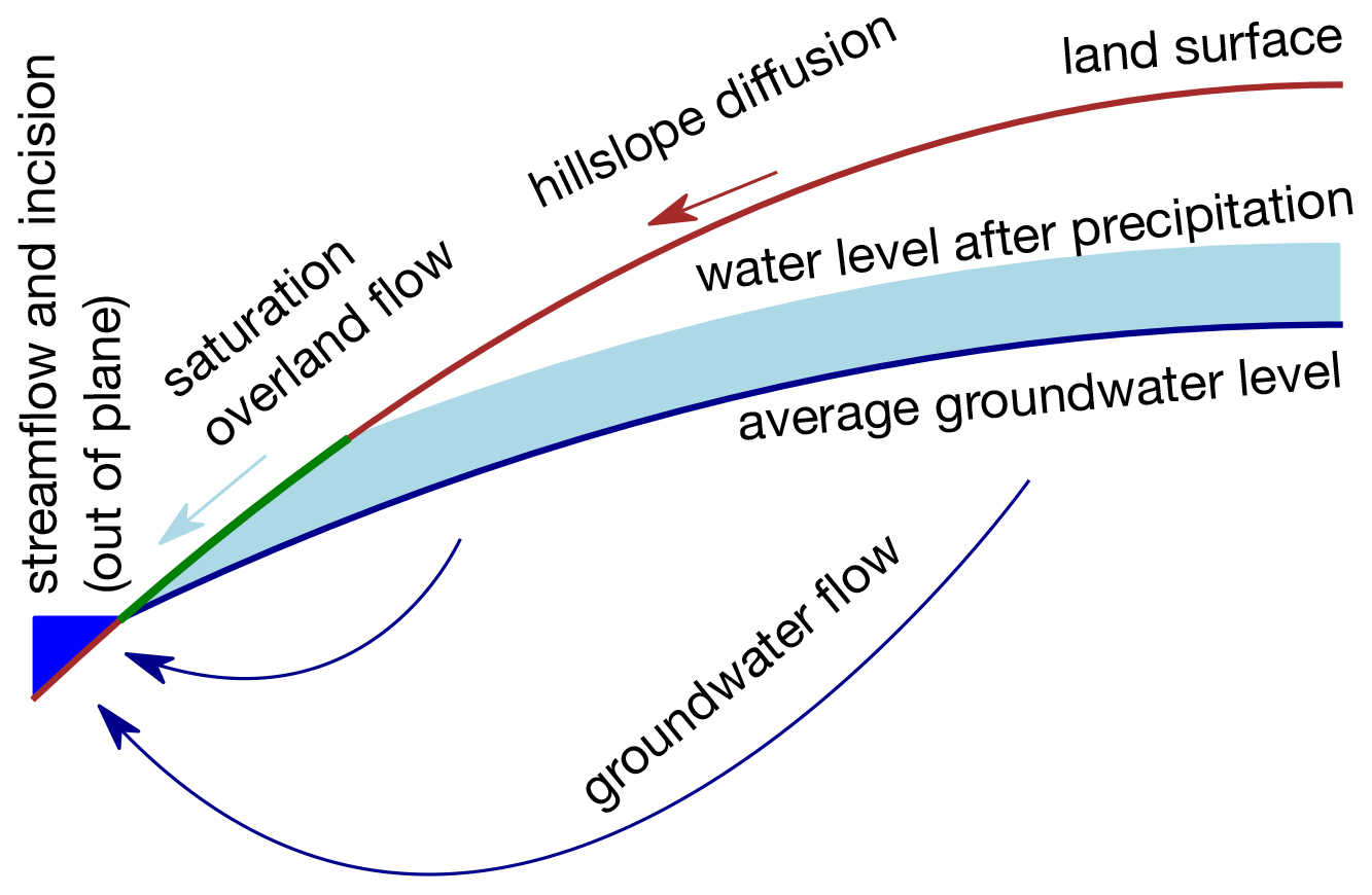
Figure 1 Conceptual model showing the hydrological and erosion process represented in the new model code. The hydrological processes include groundwater flow, overland flow and streamflow. The erosion processes include hillslope diffusion and stream incision.

2.2 Initial topography

The model starts with a random initial topography, which is calculated as using a series of 400 linear segments with random placement and random perturbation of the elevation at the start and end points of the segments. For the model simulations shown in this study, the average initial elevation is 0 m and the initial relief is 0.5 m.

2.3 Precipitation

Precipitation events are quantified using rainfall intensity statistics for the Netherlands (Beersma et al., 2019), utilizing a precipitation–frequency curve shown in Fig. 2. The rainfall intensity curves follow a generalized extreme value distribution with the parameters given by the following equations (Beersma et al., 2019):

$$\begin{array}{}\text{(1)}& {\displaystyle }\mathit{\eta }=\mathrm{1.02}{\left(\mathrm{0.239}-\mathrm{0.0250}\log (D/\mathrm{60}.)\right)}^{-\mathrm{1}/\mathrm{0.512}}\text{(2)}& {\displaystyle }\mathit{\gamma }=\mathrm{0.478}-\mathrm{0.0681}\log \left(D\right)\text{(3)}& {\displaystyle }\mathit{\kappa }=\mathrm{0.118}-\mathrm{0.266}\log \left(D\right)+\mathrm{0.0586}\left(\log \right(D{)}^{\mathrm{2}}).\end{array}$$

Here, η is the location parameter, γ is the dispersion parameter, κ is the shape parameter of the distribution and D is the duration of each rainfall event (s). For the model experiments shown in this study, a rainfall duration (D) of 3 h is used. The precipitation depth for a single precipitation event is calculated as follows:

$$\begin{array}{}\text{(4)}& P_{\mathrm{d}}=\mathrm{1000.0}\mathit{\eta }\left(\mathrm{1.0}+\mathit{\gamma }/\mathit{\kappa }(\mathrm{1.0}-T^{-\mathit{\kappa }})\right),\end{array}$$

where P_d is the rainfall depth per event (m), and T is repetition time (a), which is the reciprocal of precipitation frequency f (a⁻¹). The model simulates overland flow and groundwater recharge for an average year. The total number of precipitation events in a single year is found by adding up a series of precipitation events until the sum of the individual events matches a desired volume for the total annual precipitation (P_t):

$$\begin{array}{}\text{(5)}& P_{\mathrm{t}}=\sum _{i=f_{\mathrm{1}}}^{i=f_{\mathrm{2}}}\left(P_{\mathrm{d}}\left(i\right)f\left(i\right)\right).\end{array}$$

The precipitation events per year are calculated starting with a frequency (f₁) of 1 a⁻¹. Subsequently, higher-frequency (and lower-magnitude) events are added progressively until the desired amount of total precipitation per year is reached. The precipitation statistics are based on an average humid climate, such as the Netherlands, with a total precipitation (P_t) of 0.75 m a⁻¹.

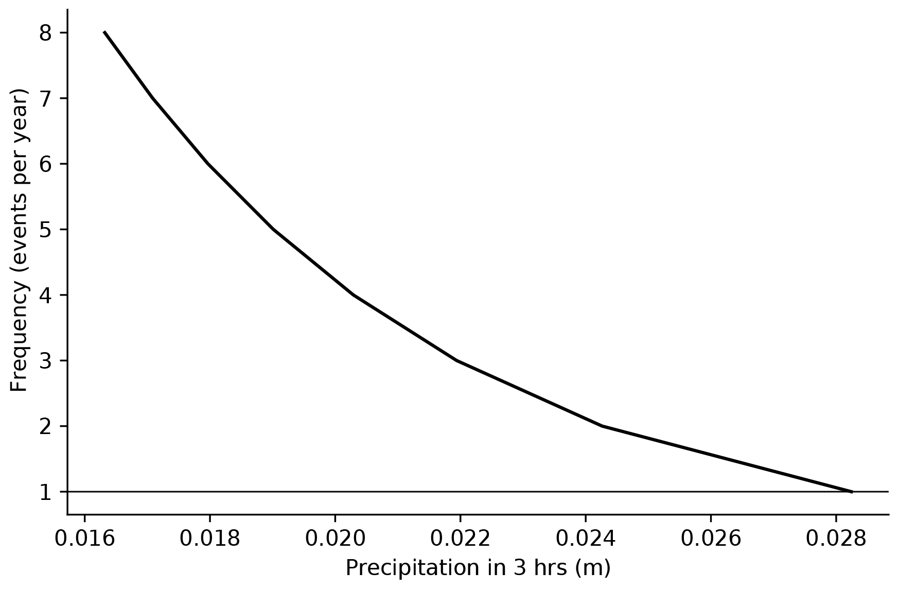
Figure 2 Precipitation–frequency curve for the Netherlands, following Beersma et al. (2019), for precipitation events with a duration of 3 h. This curve was used to model precipitation, groundwater recharge and overland flow.

2.4 Partitioning of groundwater and overland flow

The subdivision of precipitation between evapotranspiration, overland flow and groundwater flow in the model is calculated for individual precipitation events. For each precipitation event, groundwater recharge is assumed to equal the available storage in the unsaturated zone (i.e. all groundwater stored in the unsaturated zone is assumed to eventually percolate to the groundwater table). For each point in the model domain, the available storage in the unsaturated zone is calculated using the depth of the water table and the specific yield of the subsurface:

$$\begin{array}{}\text{(6)}& s=S_{\mathrm{y}}(z-h),\end{array}$$

where s is storage (m), S_y is specific yield (dimensionless), z is the elevation of the land surface (m) and h is the elevation of the water table (m). Groundwater recharge for a single precipitation event is calculated as follows:

$$\begin{array}{}\text{(7)}& {\displaystyle }{R}_i=\left\{\begin{array}{ll}s& \text{if}s<P_{\mathrm{d}}\\ P_{\mathrm{d}}& \text{if}s\mathit{>=}{P}_{\mathrm{d}}\end{array}\right.,\end{array}$$

where P_d is the precipitation depth per event (m), and R_i is the groundwater recharge depth per event (m),

The time-averaged potential recharge rate $\stackrel{\mathrm{‾}}{R_{\mathrm{p}}}$ (m s⁻¹) is calculated as the sum of the individual recharge events as follows:

$$\begin{array}{}\text{(8)}& \stackrel{\mathrm{‾}}{R_{\mathrm{p}}}=\left(\sum _{i=\mathrm{11}}^{i=n}\left(R_i{f}_i\right)\right)/\mathrm{\Delta }{t}_{\mathrm{r}},\end{array}$$

where f_i is the frequency of precipitation event i (s⁻¹), and Δt_r is the duration of the reference time period, which is 1 year (s). The actual recharge rate is calculate by subtracting evapotranspiration:

$$\begin{array}{}\text{(9)}& {\displaystyle }R=\left\{\begin{array}{ll}{R}_{\mathrm{p}}-\mathrm{ET}& \text{if}{R}_{\mathrm{p}}>\mathrm{ET}\\ \mathrm{0}& \text{if}{R}_{\mathrm{p}}\le \mathrm{ET}\end{array}\right.,\end{array}$$

where ET is the evapotranspiration rate (m s⁻¹). Note that, for simplicity, the evapotranspiration rate is assumed to be a fixed value and independent of the depth of the water table.

Saturation overland flow is calculated as the amount of precipitation that exceeds the available storage (s) in the unsaturated zone. For each node in the model domain and for each precipitation event, the saturation overland flow depth is calculated as follows:

$$\begin{array}{}\text{(10)}& {\displaystyle }{Q}_{si}=\left\{\begin{array}{ll}{P}_{\mathrm{d}}-S& \text{if}s<P_{\mathrm{d}}\\ \mathrm{0}& \text{if}s\mathit{>=}{P}_{\mathrm{d}}\end{array}\right.,\end{array}$$

where Q_si is the saturation overland flow depth per precipitation event (m).

2.5 Groundwater flow

The model is based on the assumption that groundwater flow can be considered to be in steady state on the timescales of stream and hillslope erosion processes. This was judged to be reasonable because the groundwater flow system reacts much faster than the relatively slow rates of erosion. Given these assumptions, groundwater flow and the position of the water table can be calculated using analytical solutions of steady-state groundwater flow.

First, the out-of-plane component of groundwater flow (i.e. groundwater flow parallel to the direction of the nearest stream) is calculated using Darcy's equation and assuming that the out-of-plane hydraulic gradient is equal to the (out-of-plane) slope of the nearest stream:

$$\begin{array}{}\text{(11)}& Q_{\mathrm{go}}=TS,\end{array}$$

where T is transmissivity (m² s⁻¹), and S is stream slope (m m⁻¹). Out-of-plane groundwater flow can be significant for cases with high transmissivity or stream slope, as shown in Fig. 3.

Figure 3 Calculated out-of-plane groundwater flow for a range of values of transmissivity and stream slope, using the base-case values of the contributing area (5 km) and groundwater recharge (0.375 m a⁻¹).

The remaining in-plane groundwater flow (i.e. towards the nearest stream) is calculated using the value of recharge calculated in Eq. (8) and subtracting the out-of-plane discharge:

$$\begin{array}{}\text{(12)}& R_{\mathrm{e}}=\stackrel{\mathrm{‾}}{R}{L}_{\mathrm{u}}-Q_{\mathrm{go}},\end{array}$$

where R_e is the effective in-plane recharge (m s⁻¹), and L_u is the length of the upstream contributing area (m).

In-plane groundwater flow is calculated using the Dupuit–Forchheimer equation, which describes depth-integrated steady-state groundwater flow between two groundwater discharge points (Forchheimer, 1886; Bresciani et al., 2016):

$$\begin{array}{}\text{(13)}& \mathrm{\Delta }h={\displaystyle \frac{\stackrel{\mathrm{‾}}{R_{\mathrm{e}}}}{\mathrm{2}T}}x(L-x)+\mathrm{\Delta }Hx/L,\end{array}$$

where h is the hydraulic head (m), L is the distance between two groundwater discharge points (m), x is the distance to the first discharge point (m) and ΔH is the difference in water level between the two discharge points (m). The term groundwater discharge point represents a point such as a stream or a part of the land surface where the water table is at the surface and where groundwater seepage takes place. The equation assumes that the lateral differences in the hydraulic head (h) are much smaller than the thickness of the aquifer (Bresciani et al., 2016).

For points at the edge of the model domain that are only bound by a discharge point on one side, the equation reduces to

$$\begin{array}{}\text{(14)}& \mathrm{\Delta }h={\displaystyle \frac{\stackrel{\mathrm{‾}}{R_{\mathrm{e}}}}{T}}x(L_{\mathrm{b}}-\mathrm{0.5}x),\end{array}$$

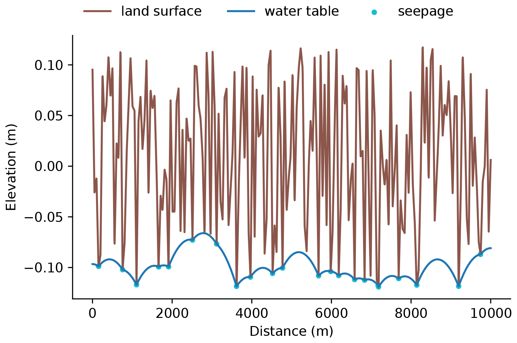
where L_b is the distance between the discharge point and the lateral model boundary (m). The average in-plane groundwater recharge rate $\stackrel{\mathrm{‾}}{R_{\mathrm{e}}}$ was calculated as the average effective recharge rate for all the nodes in between two seepage nodes. The seepage nodes represent points where the water table is at the surface and where groundwater discharge occurs. The position of the seepage nodes is not known in advance; instead, it is calculated using the following iterative procedure:

1. First, one seepage node is picked at the lowest elevation in the model domain, and the water table is calculated using Eqs. (13) and (14). In most cases, the calculated water table is still above the land surface in a large part of the model domain after the first iteration.

2. Subsequently, a new seepage node is added at the node with the lowest elevation in the part of the model domain where the modelled water table exceeds the land surface.

3. The water table is recalculated using this new additional seepage node.

4. The last two steps are repeated until the modelled water table is below or at the land surface (i.e. h≤z) everywhere.

An example of the calculated water table and seepage locations following the procedure is shown in Fig. 4.

Figure 4 Example of initial topography and calculated water table and groundwater seepage locations. The water table and seepage locations were calculated by an iterative solution of Eqs. (13) and (14), as explained in Sect. 2.5.

2.6 Streamflow

The water flow in each stream consists of two components: (1) steady baseflow supplied by groundwater discharge and (2) transient flow that consists of overland flow. The calculation of both components is described in the following two sections.

2.6.1 Baseflow

The baseflow in each stream node is calculated in two steps. First, streams nodes are found by finding the node with the lowest elevation for each series of neighbouring seepage nodes in the model domain. Note that the term seepage nodes is used here to denote nodes where groundwater discharge occurs. The 2D (in-plane) value of groundwater flow toward each stream node (q_b) is calculated for each stream by finding the nodes contributing groundwater to each stream and by summing the product of the recharge rate at each node R and the width of each node (Δx). The contributing area is found by the taking the water table h as calculated using Eqs. (13) and (14) and finding the two nodes on either side of each stream where the hydraulic gradient changes direction. The 3D (out-of-plane) value of baseflow was calculated by multiplying in-plane baseflow (q_b) by an upstream length of each stream:

$$\begin{array}{}\text{(15)}& Q_{\mathrm{b}}=q_{\mathrm{b}}{L}_u,\end{array}$$

where Q_b is baseflow. An example of the calculated value of baseflow is shown in Fig. 5.

Figure 5 Example of calculated baseflow to streams. The coloured triangles denote the magnitude of the calculated baseflow.

2.6.2 Saturation overland flow

The volume of water that is contributing to overland flow is calculated per precipitation event as follows:

$$\begin{array}{}\text{(16)}& V_{\mathrm{0}}=\underset{x_{\mathrm{1}}}{\overset{x_{\mathrm{2}}}{\int }}{Q}_{\mathrm{si}}\mathrm{d}x,\end{array}$$

where V₀ is the volume of water to be discharged in a stream channel (m³), x₁ and x₂ are the positions of the topographic divide on either side of the channel (m), and Q_si is the rate of overland flow for each node as calculated using Eq. (10). An example of the resulting distribution of precipitation excess and overland flow is shown in Fig.  6.

Figure 6 Example of calculated precipitation excess and saturation overland flow in streams. Panel (a) shows the calculated precipitation excess for each node in the model domain. Panel (b) shows the location of nodes where the precipitation depth for a single event exceeds the available storage, which results in fully saturated conditions and the generation of saturation overland flow. Panel (c) shows the calculated saturation overland flow volume for each stream in the model domain. Note that all of the potential streams are shown here, including potential streams in depressions that do not generate overland flow because they are located too far above the water table.

2.6.3 Water level in streams

The water level in streams as a result of baseflow and overland flow is calculated using the Gauckler–Manning equation for stream discharge. The Gauckler–Manning equation for stream discharge is as follows (Gauckler, 1867; Manning, 1891):

$$\begin{array}{}\text{(17)}& v=K_n{R}^{\mathrm{2}/\mathrm{3}}{S}^{\mathrm{1}/\mathrm{2}},\end{array}$$

where v is the mean flow velocity in a stream channel (m s⁻¹); K_n is an empirical coefficient (${\mathrm{m}}^{\mathrm{1}/\mathrm{3}}{\mathrm{s}}^{-\mathrm{1}}$) that is defined as $\mathrm{1}/n$, where n is the Manning's roughness coefficient ($\mathrm{s}{\mathrm{m}}^{-\mathrm{1}/\mathrm{3}}$); R is hydraulic radius (m); and S is the slope of the water surface, which is assumed to be equal to the slope of the channel bed (m m⁻¹). With the common assumption that channels are much wider than they are deep, R≈h_c and the equation can be simplified to

$$\begin{array}{}\text{(18)}& v=K_n{S}^{\mathrm{1}/\mathrm{2}}{h}_{\mathrm{c}}^{\mathrm{2}/\mathrm{3}},\end{array}$$

where h_c is the water height in the channel (m). The discharge is equal to the product of the flow velocity and the cross-sectional area. To simplify the equations the cross section for each stream is assumed to be triangular. The linear in-plane slope of the channel bed (i.e. perpendicular to the flow direction in the channel) is denoted as S_t (m m⁻¹). The cross-sectional area of the channel equals S_th². Using this, the discharge equation can be written as follows:

$$\begin{array}{}\text{(19)}& Q_{\mathrm{w}}={\displaystyle \frac{K_n{S}^{\mathrm{1}/\mathrm{2}}}{S_t}}{h}_{\mathrm{c}}^{\mathrm{8}/\mathrm{3}},\end{array}$$

where Q_w is the discharge in the channel (m³ s⁻¹). Rewriting this equation yields an expression for the water level in streams as a function of discharge:

$$\begin{array}{}\text{(20)}& h_{\mathrm{c}}={\left({\displaystyle \frac{S_t{Q}_{\mathrm{w}}}{K_n{S}^{\mathrm{1}/\mathrm{2}}}}.\right)}^{\mathrm{3}/\mathrm{8}}.\end{array}$$

2.6.4 Transient stream discharge

The discharge generated by overland flow operates on short timescales of hours to days. Modelling this process directly would require short time steps that would make the model prohibitive computational expensive. Instead, this work derives new equations for the total discharge in a stream following a single precipitation event. To keep the solution mathematically tractable, the assumption is made that each precipitation event generates a volume of overland flow that is added instantaneously to the stream channel. The volume is subsequently discharged over time.

The continuity equation for discharge of a stream channel is given by

$$\begin{array}{}\text{(21)}& {\displaystyle \frac{\partial V_{\mathrm{w}}}{\partial t}}=-Q_{\mathrm{w}},\end{array}$$

where V_w is the water volume in the channel (m³). The volume to be discharged is defined as the product of a cross-sectional area that changes over time and a fixed stream length L_u (m):

$$\begin{array}{}\text{(22)}& V_{\mathrm{w}}=A{L}_u.\end{array}$$

Assuming that the shape of the channel is a triangle and combination with the stream discharge equation (Eq. 19) yields

$$\begin{array}{}\text{(23)}& {\displaystyle \frac{L_u}{S_t}}{\displaystyle \frac{\partial h_{\mathrm{c}}^{\mathrm{2}}}{\partial t}}=-{\displaystyle \frac{K_n{S}^{\mathrm{1}/\mathrm{2}}}{S_t}}{h}_{\mathrm{c}}^{\mathrm{8}/\mathrm{3}}.\end{array}$$

Integration of this equation with boundary condition h_c=h₀ at t=0 yields

$$\begin{array}{}\text{(24)}& h_{\mathrm{c}}={\left(h_{\mathrm{0}}^{-\mathrm{2}/\mathrm{3}}+{\displaystyle \frac{K_n{S}^{\mathrm{1}/\mathrm{2}}}{\mathrm{3}L}}t\right)}^{-\mathrm{3}/\mathrm{2}}.\end{array}$$

The initial height of the water level in the channel (h₀) is related to the initial volume of water in the channel V₀:

$$\begin{array}{}\text{(25)}& V_{\mathrm{0}}={\displaystyle \frac{h_{\mathrm{0}}^{\mathrm{2}}{L}_u}{S_t}}.\end{array}$$

Adding Eq. (25) into Eq. (24) and replacing the constants yields an expression for the decrease in the water level in a channel over time in response to the drainage of an initial volume V₀:

$$\begin{array}{}\text{(26)}& h_{\mathrm{c}}={\left({{\displaystyle \frac{V_{\mathrm{0}}{S}_t}{L_u}}}^{-\mathrm{1}/\mathrm{3}}+{\displaystyle \frac{K_n{S}^{\mathrm{1}/\mathrm{2}}}{\mathrm{3}{L}_u}}t\right)}^{-\mathrm{3}/\mathrm{2}}.\end{array}$$

This equation was validated by comparison with a numerical solution for the water level over time (Fig. 7). The numerical solution was calculated using the discharge equation (Eq. 19) to calculate discharge over time. At the first time step, the initial overland flow volume V₀ is added. Subsequently, discharge is calculated and subtracted from the initial volume V₀. The height of the water level at each time step was calculated using Eq. (25). This process is repeated until the water level is less than 1 mm.

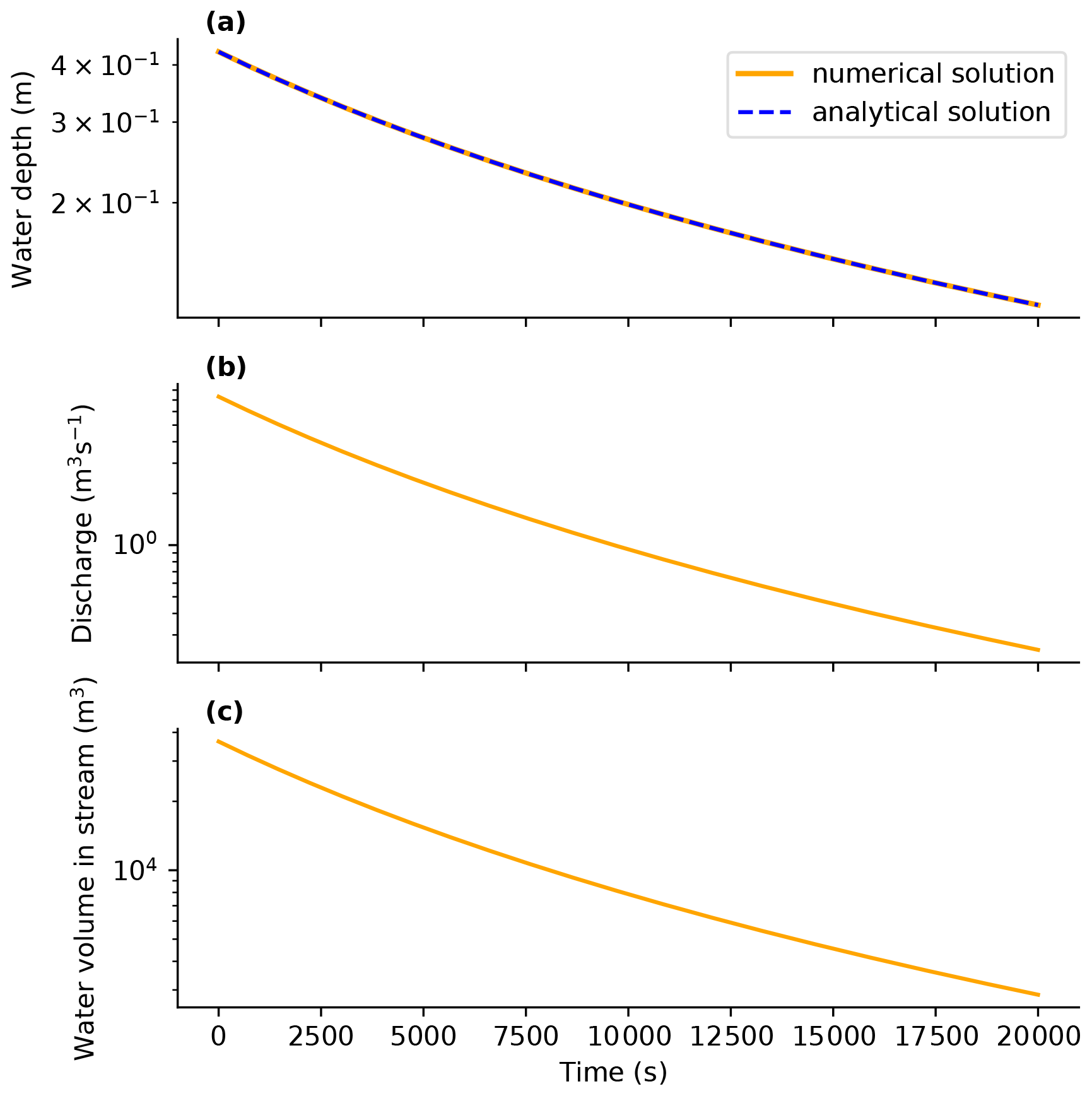
Figure 7 Validation of the equation for the transient discharge of an instantaneously added volume of water in a stream channel (Eq. 26) using the numerical solution as described in the text. Panel (a) shows that the numerical solution and analytical solution overlap perfectly. Panels (b) and (c) show the change in water volume and discharge in the channel over time, which were used to calculate the numerical solution in panel (a). The solution uses the base-case parameters listed in Table 1; a precipitation depth of 0.0365 m, which is the theoretical maximum 1 d precipitation depth for a return time of 1 year for the Netherlands; and a contributing area for overland flow with a length of 100 m.

2.7 Stream incision

The sediment flux in a stream channel at carrying capacity is given by the following equation (Tucker and Bras, 1998; Tucker and Hancock, 2010):

$$\begin{array}{}\text{(27)}& Q_{\mathrm{s}}=w{k}_f(Q_{\mathrm{w}}/w{)}^m{S}^n,\end{array}$$

where Q_s is the sediment flux (m³ s⁻¹), w is channel width (m), k_f is the sediment transport coefficient (${\mathrm{s}}^{\mathrm{4}/\mathrm{5}}{\mathrm{m}}^{-\mathrm{8}/\mathrm{5}}$), Q_w is water discharge (${\mathrm{m}}^{-\mathrm{3}}{\mathrm{s}}^{-\mathrm{1}}$) and S is channel slope (dimensionless); m and n are the respective discharge exponent (dimensionless) and slope exponent (dimensionless), which were set to values of 1.8 and 2.1 respectively. The erosion by streams is subdivided into two components: (1) the erosion by baseflow driven by groundwater discharge and (2) the additional transient erosion by saturation overland flow during and directly after precipitation events. In addition, incision and stream slope are governed by the base level. The equations for the calculation of the base level and the two erosion components are discussed in the following sections.

2.7.1 Base-level change

The incision of streams results in an adjustment of the stream slope (S). The stream slope is also dependent on changes in the base level. The base level at the downstream boundary of the model domain is calculated as follows:

$$\begin{array}{}\text{(28)}& z_{\mathrm{b}}=z_{\mathrm{b},\mathrm{0}}+Ut,\end{array}$$

where z_b is the elevation of the downstream model boundary (m), U is the base-level change rate (m s⁻¹) and t is the total elapsed time since the start of the model run (s). z_b,0 (m) is the initial base level at the start of the model run and is calculated as the product of initial stream slope and distance to the downstream model boundary:

$$\begin{array}{}\text{(29)}& z_{\mathrm{b},\mathrm{0}}=z_{\mathrm{0}}+S_{\mathrm{0}}{L}_{\mathrm{d}}.\end{array}$$

Here, z₀ is the average elevation in the cross section at t=0 (m), which is 0 m for the model runs shown in this study; S₀ is the initial slope (m m⁻¹); and L_d is the distance to the downstream model boundary (m).

After each time step, a new value of stream slope is calculated using the new elevation of the base of the stream and the elevation of the downstream edge of the model domain:

$$\begin{array}{}\text{(30)}& S={\displaystyle \frac{z_{\mathrm{s}}-z_{\mathrm{b}}}{L_{\mathrm{d}}}},\end{array}$$

where z_s is the elevation of the stream in the modelled cross section (m).

2.7.2 Stream incision by baseflow

The sediment flux in the steam channel carried by baseflow is calculated using Eq. (27), with the value of baseflow calculated using Eq. (15) as the value for water discharge Q_w. The incision of the stream is calculated by dividing the sediment flux by the channel width (w). In addition, the erosion is divided over the upstream length of the stream by assuming that erosion increases linearly from zero at the start of the stream to the maximum value at the end of the stream. This yields the following equation for erosion of the stream channel:

$$\begin{array}{}\text{(31)}& {\displaystyle \frac{\partial z}{\partial t}}=(\mathrm{1}-\mathit{\varphi }){\displaystyle \frac{Q_s}{w\frac{\mathrm{1}}{\mathrm{2}}{L}_u}},\end{array}$$

where z is the elevation of the base of the channel (m), t is time (s) and ϕ is porosity (dimensionless). Note that the linear increase in erosion by baseflow along the stream is a simplification that makes the problem more tractable mathematically. In reality, the non-linear relation between streamflow and erosion would result in a non-linear increase in erosion along the stream profile. Channel width was calculated as follows (Lacey, 1930):

$$\begin{array}{}\text{(32)}& w=k_{\mathrm{w}}{Q}^{\mathit{\omega }},\end{array}$$

where k_w and ω are empirical parameters that are set to values of 3.65 and 0.5 respectively (van den Berg, 1995).

2.7.3 Stream incision by overland flow

Erosion by streams caused by the discharge of overland flow is calculated by combining the equation for stream discharge due to overland flow over time (Eq. 26) with the sediment discharge equation (Eq. 27). The combination of these two equations yields

$$\begin{array}{}\text{(33)}& Q_s=k_f{S}^n{\left({\displaystyle \frac{K_n{S}^{\mathrm{1}/\mathrm{2}}}{S_t}}\right)}^m{\left({\left({\displaystyle \frac{V_{\mathrm{0}}{S}_t}{L_u}}\right)}^{-\mathrm{1}/\mathrm{3}}+{\displaystyle \frac{K_n{S}^{\mathrm{1}/\mathrm{2}}}{\mathrm{3}{L}_u}}t\right)}^{-\mathrm{4}m}.\end{array}$$

Integrating this equation from t=0 to t=∞ yields an expression for the total volume of sediment eroded from the channel after a single precipitation and discharge event:

$$\begin{array}{}\text{(34)}& V_{\mathrm{s}}={\displaystyle \frac{a(b+c{)}^{(-\mathrm{4}m+\mathrm{1})}}{\mathrm{4}mc+c}},\end{array}$$

where V_s is the total volume eroded in a stream by overland flow following a single precipitation event, and a, b and c are constants that are defined as

$$\begin{array}{}\text{(35)}& {\displaystyle }a=k_f{S}^n{\left({\displaystyle \frac{K_n{S}^{\mathrm{1}/\mathrm{2}}}{S_t}}\right)}^m\text{(36)}& {\displaystyle }b={\left({\displaystyle \frac{V_{\mathrm{0}}{S}_t}{L_u}}\right)}^{-\mathrm{1}/\mathrm{3}}\text{(37)}& {\displaystyle }c={\displaystyle \frac{K_n{S}^{\mathrm{1}/\mathrm{2}}}{\mathrm{3}{L}_u}}.\end{array}$$

The eroded volume results in incision of the stream. Stream incision by overland flow is calculated by distributing the eroded volume (V_s) evenly over the width of the stream channel (w). In addition, erosion by overland flow is assumed to increase linearly from the start of the channel to the position of the modelled cross section. This is a similar simplification to the linear increase in erosion by baseflow discussed in the previous section, and it was also used to keep the problem mathematically tractable. This yields the following expression for the incision of the stream due to overland flow:

$$\begin{array}{}\text{(38)}& \mathrm{\Delta }{z}_{\mathrm{s}}={\displaystyle \frac{V_{\mathrm{s}}}{\left(w\frac{\mathrm{1}}{\mathrm{2}}{L}_u\right)}},\end{array}$$

where Δz_s is stream incision following a single precipitation event (m).

2.8 Hillslope diffusion

Erosion of the parts of the model domain outside of the streams follows the hillslope diffusion equation (Culling, 1960):

$$\begin{array}{}\text{(39)}& {\displaystyle \frac{\partial z}{\partial t}}={\displaystyle \frac{\partial \left(K_{\mathrm{d}}\frac{\partial z}{\partial x}\right)}{\partial x}},\end{array}$$

where K_d is the hillslope diffusion coefficient (m² s⁻¹). This equation was solved numerically with a standard implicit finite difference approach using a matrix solver implemented in the NumPy Python module (Harris et al., 2020).

2.9 Iterative solution

The solution of the equations for groundwater flow, overland flow, streamflow and erosion follow an iterative scheme that is detailed in Fig. 8. After setting up an initial topography, the initial water table is calculated using the procedure described in Sect. 2.5, with recharge taken as the difference between the total precipitation (P_t), overland flow and evapotranspiration (ET). Subsequently, the model calculates baseflow, stream incision due to baseflow and overland flow, and topography change due to hillslope diffusion. Overland flow and recharge are calculated on an event basis. Recharge is summed over a year in order to yield an average recharge rate. Overland flow and erosion are calculated on an event basis and are then summed over a year in order to yield an average overland flow erosion rate. This procedure is repeated at each time step. The initial time step size is 1 year. The time step size was adjusted so that the maximum elevation change per time step was 0.5 % of the total relief with a minimum of 0.01 m. These conditions were found by trial and error to ensure numerically stable and computationally efficient model runs for the range of parameter values and runs reported in this study.

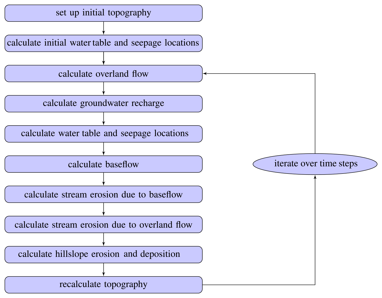
Figure 8 Flow chart for the iterative solution of the groundwater flow, overland flow and erosion equations.

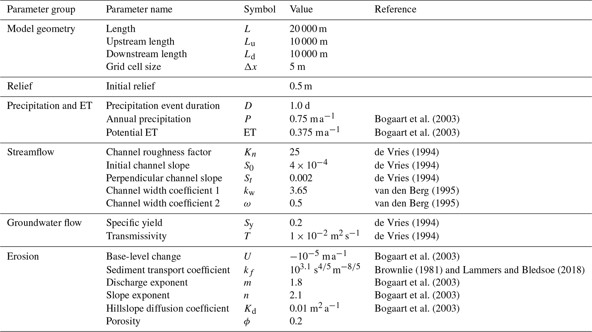
2.10 Base-case parameter values

The base-case parameter values follow de Vries (1994) and Bogaart et al. (2003), who modelled stream network and landscape evolution of the southern Netherlands under alternating glacial and interglacial conditions. Here, the parameters that represent present-day (interglacial) conditions are used. The base-case parameters are listed in Table 1. In contrast to the relatively high value for porosity of 0.4 used by Bogaart et al. (2003), a value of 0.2 is used here, which more closely follows values observed in areas covered by fluvial and aeolian sediments in the southern Netherlands (de Vries, 1994). The base-case value for transmissivity is $\mathrm{1}\times {\mathrm{10}}^{-\mathrm{2}}$ m² s⁻¹, which is based on values that range from 0.012 to 0.03 m² s⁻¹ reported by de Vries (1994). The initial slope value of $\mathrm{5}\times {\mathrm{10}}^{-\mathrm{4}}$ m m⁻¹ is equal to the average stream gradient in the southern Netherlands.

The value of the sediment transport coefficient reported by Bogaart et al. (2003) was based on the theoretical Einstein–Brown equation. Here, the value of this parameter is based on an analysis of alluvial sediment discharge data by Brownlie (1981), as reported by Lammers and Bledsoe (2018). Following the sediment discharge equation (Eq. 27), the sediment transport coefficient (k_f) can be expressed as

$$\begin{array}{}\text{(40)}& k_f={\displaystyle \frac{q_{\mathrm{s}}}{q_{\mathrm{w}}^m{S}^n}}.\end{array}$$

The compilation of total sediment discharge from flume experiments and field observations by Brownlie (1981), as reported by Lammers and Bledsoe (2018), contains n=1463 data points for which sediment discharge (q_s), water discharge (q_w) and stream slope (S) are known. Following Bogaart et al. (2003), the coefficients n and m are set to values of 1.8 and 2.1 respectively. Inserting these values into Eq. (40) allows k_f to be calculated for each of the 1463 data points. The calculated distribution of k_f using Eq. (40) is shown in Fig. 9. Comparison of the measured sediment discharge values and the denominator ($q_{\mathrm{w}}^m{S}^n$) in Eq. (40) shows that there is a reasonable correlation of the term $q_{\mathrm{w}}^m{S}^n$ with the sediment discharge rate. When using the median value of k_f=10^3.1 to predict sediment discharge, the coefficient of determination for log-transformed values of sediment discharge equals 0.62. The median value of k_f=10^3.1 was used as the base-case parameter value for the model experiments shown in this study. Note that more complex sediment transport equations that consider sediment grain size and transport thresholds yield a closer fit to the data (Lammers and Bledsoe, 2018). However, these equations were not implemented in this study to keep the calculation of sediment discharge for individual discharge events (Eq. 34) mathematically tractable.

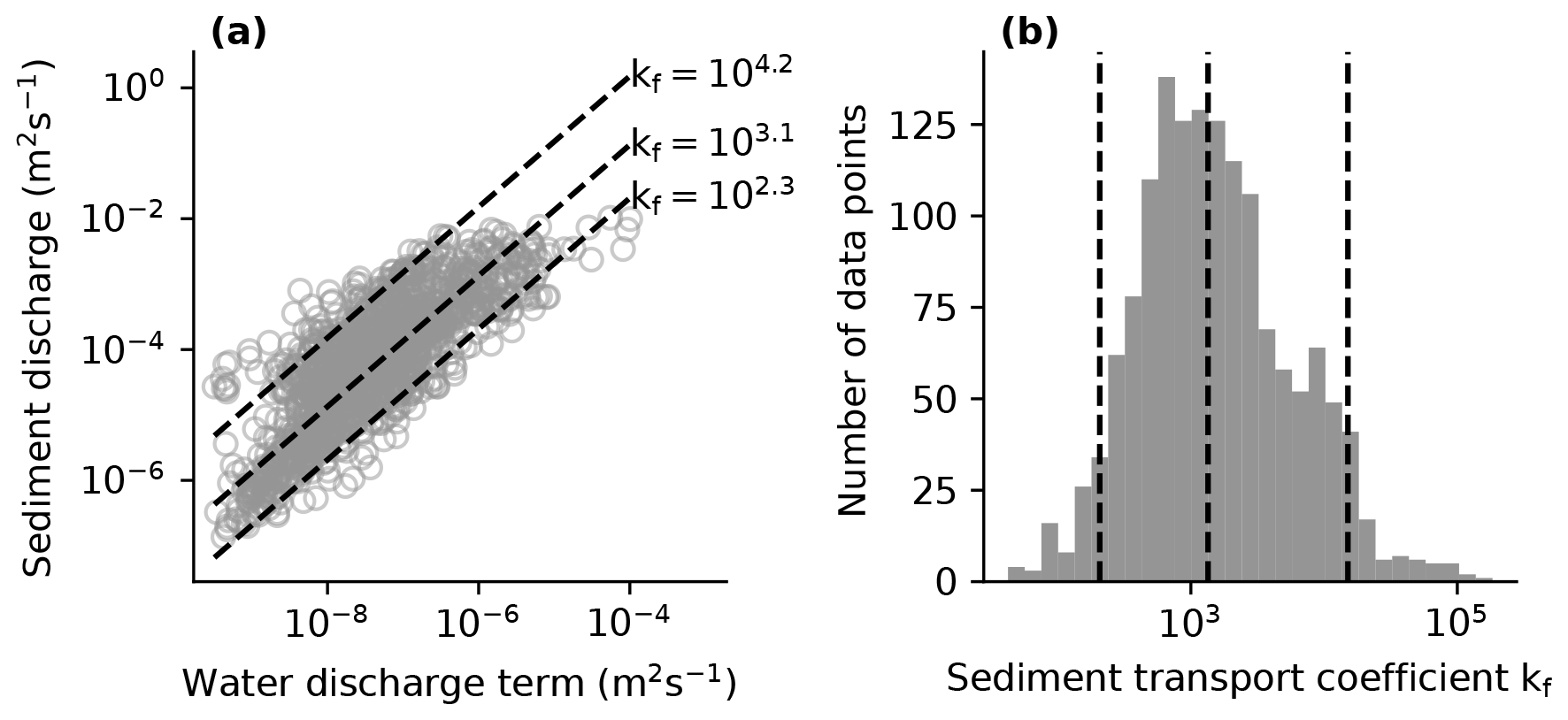
Figure 9 Comparison of measured sediment discharge and the water discharge term $q_{\mathrm{w}}^m{S}^n$ in the sediment discharge equations (Eqs. 27 and 40) (a) and the calculated variation of the sediment transport coefficient (b) in a compilation of 1463 sediment discharge data from flume experiments and field observations by Brownlie (1981), as reported by Lammers and Bledsoe (2018). The lines in panels (a) and (b) denote the 0.05, 0.5 and 0.95 quantiles of the distribution of k_f as calculated using Eq. (40).

Bogaart et al. (2003)Bogaart et al. (2003)de Vries (1994)de Vries (1994)de Vries (1994)van den Berg (1995)van den Berg (1995)de Vries (1994)de Vries (1994)Bogaart et al. (2003)Brownlie (1981)Lammers and Bledsoe (2018)Bogaart et al. (2003)Bogaart et al. (2003)Bogaart et al. (2003)

Table 1 Base-case parameter values.

2.11 Model sensitivity analyses

To explore the role of groundwater flow in erosion, a series of model experiments were conducted with different values for transmissivity and specific yield. To compare the effects of changes in groundwater flow with climate and erosion parameters, an additional set of experiments was conducted with different values for total precipitation (P_t), hillslope diffusion coefficient (K_d), sediment transport coefficient (k_f) and base-level change (U). These values are listed in Table 2.

The range of variation in the hillslope diffusion coefficient was based on Richardson et al. (2019). There is no large compilation of transmissivity data available. Models and data of the permeability of unconsolidated sediments (Gleeson et al., 2011; Luijendijk and Gleeson, 2015) and a hydrologically active layer of approximately 100 m (Gleeson et al., 2016; Jasechko et al., 2017) suggest a variation of approximately 10⁻⁷ to 10⁻¹ m² s⁻¹. Here, a smaller range of values is evaluated (10⁻⁴ to 10⁻¹ m) because, for the relatively low-relief landscape that was studied, lower values of transmissivity result in drainage densities that are fully controlled by the initial random topography. The values of specific yield are based on values reported for mixed sediments (Revil, 2002; Gleeson et al., 2014; El-husseiny, 2020). The minimum and maximum values for the sediment transport coefficient were equal to the 0.05 and 0.95 quantiles of the calculated distribution of k_f shown in Fig. 9.

Table 2 Parameter value range in model sensitivity analyses.

2.12 Additional model experiments

In addition to the model sensitivity analysis, a second set of model experiments was conducted to explore the persistence of drainage density over longer timescales. These model experiments used the modelled incised topography of the base-case model run after 10 000 years as a starting point and subsequently added another 50 000 years to the simulation, although with different parameter values that follow the sensitivity analysis reported in the previous section and Table 2. These different parameter values resulted in model simulations where the system was out of balance with the incised topography. The degree to which these runs resulted in an adjustment of the stream network and drainage density after a runtime of 10 000 and 50 000 years was recorded and used to quantify the persistence of stream networks.

3 Results

3.1 Groundwater capture

Figure 10 shows the result of an example model run using the base-case parameter values as shown in Table 1. The figure shows the evolution of the land surface from an initial randomly generated surface over a time span of 10 000 years. The system starts out with a very high drainage density, with 114 streams in a model domain that is 20 km long. Subsequently, the model evolves rapidly towards a system dominated by fewer streams over time, with the final number of 12 active streams after a runtime of 10 000 years.

The decrease in number of streams is caused by a process that is defined here as groundwater capture, by which faster eroding streams draw the water table below neighbouring streams and reduce the baseflow and saturation overland flow of these streams until they become dry. The process of groundwater catchment capture is illustrated in more detail in Fig. 11, which shows the land surface, water table and stream fluxes for three time slices before, during and after a groundwater catchment capture event. After 2251 kyr (Fig. 11a), 13 streams are still active. However, the last stream on the right-hand side has a smaller catchment area and a lower baseflow and, therefore, incises slower than its neighbouring stream. After 2457 years (Fig. 11b), the neighbouring stream has incised further and has drawn the water table below the base of the stream. The stream does generate overland flow but has ceased to generate baseflow. At 2707 years, the water table has been drawn down further and is too deep for the stream to generate saturation overland flow (i.e. all of the precipitation that falls near the stream can be accommodated in the unsaturated zone above the water table). As a result, the stream has become inactive. The stream channel has partly been filled by hillslope diffusion, as the sediment flux caused by hillslope diffusion is no longer compensated for by the removal of sediment by streamflow.

The evolution of the stream network over time is summarized in Fig. 12. Initially, each small depression is potentially an active stream channel, which results in a large number of active streams. However, as the incision of streams increases, the number of active streams drops rapidly in the first 100 years, followed by a slower reduction in the number of active streams. The last stream capture event at 2457 years is shown in Fig. 11. After this event, the drainage system remains in a steady state. Note that the model runtime in Fig. 12 was extended to 1 million years to show the evolution of the landscape and stream network over a long time span.

The initially high rate of groundwater capture is slowed down over time by the negative feedback imposed by the base level at the downstream (out-of-plane) end of the model domain. The stream slope is lower for streams that have incised deeper, which limits their incision power. The negative feedback on incision results in the establishment of a steady-state drainage network after 2500 years. For the base-case model run shown in Fig. 10, the base level is located at an elevation of −4 m, at a downstream distance of 10 000 m.

The incision and the reduction of active streams by groundwater capture also means that the area susceptible to saturation overland flow decreases over time, as saturation overland flow takes place near active stream channels where the water table is located close to the surface. Apart from a short phase at the start of the model run, streamflow and stream erosion are predominantly generated by groundwater flow, which is referred to as baseflow once it enters the stream channel (Fig. 12b, c).

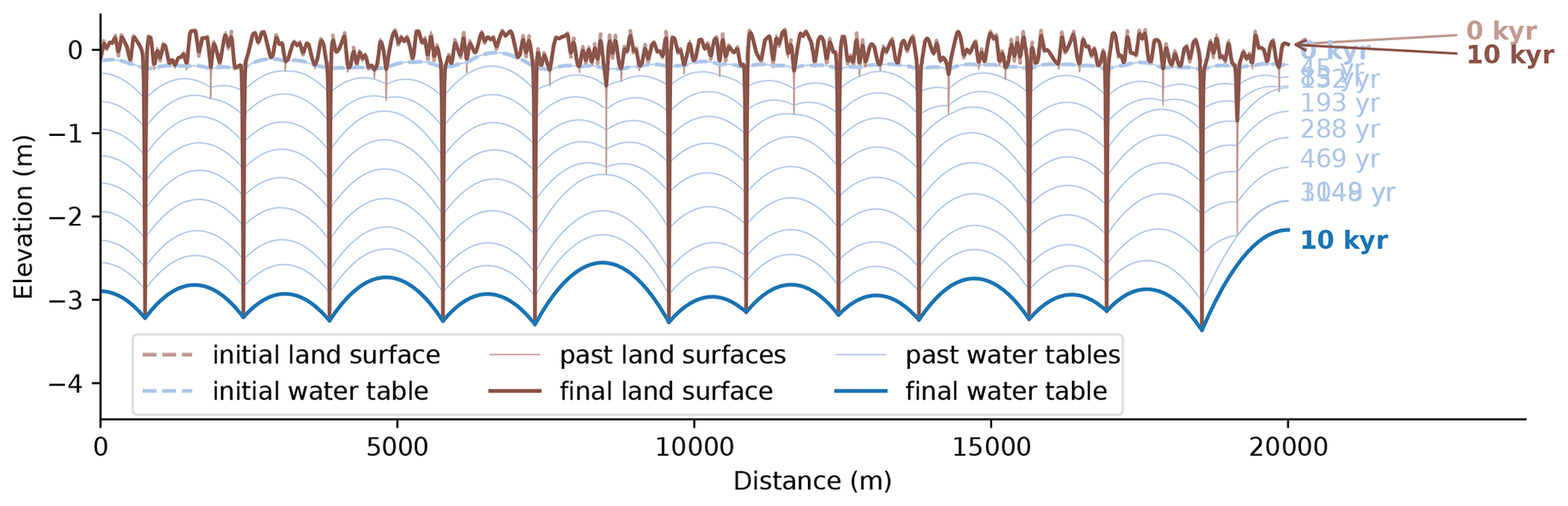
Figure 10 Modelled change in the land surface and water table over 10 000 years for the base-case model run. The results show the evolution from a random topography with a high number of streams to an incised topography with 12 active streams. The past positions of the land surface and water table show the decrease in the number of streams over time.

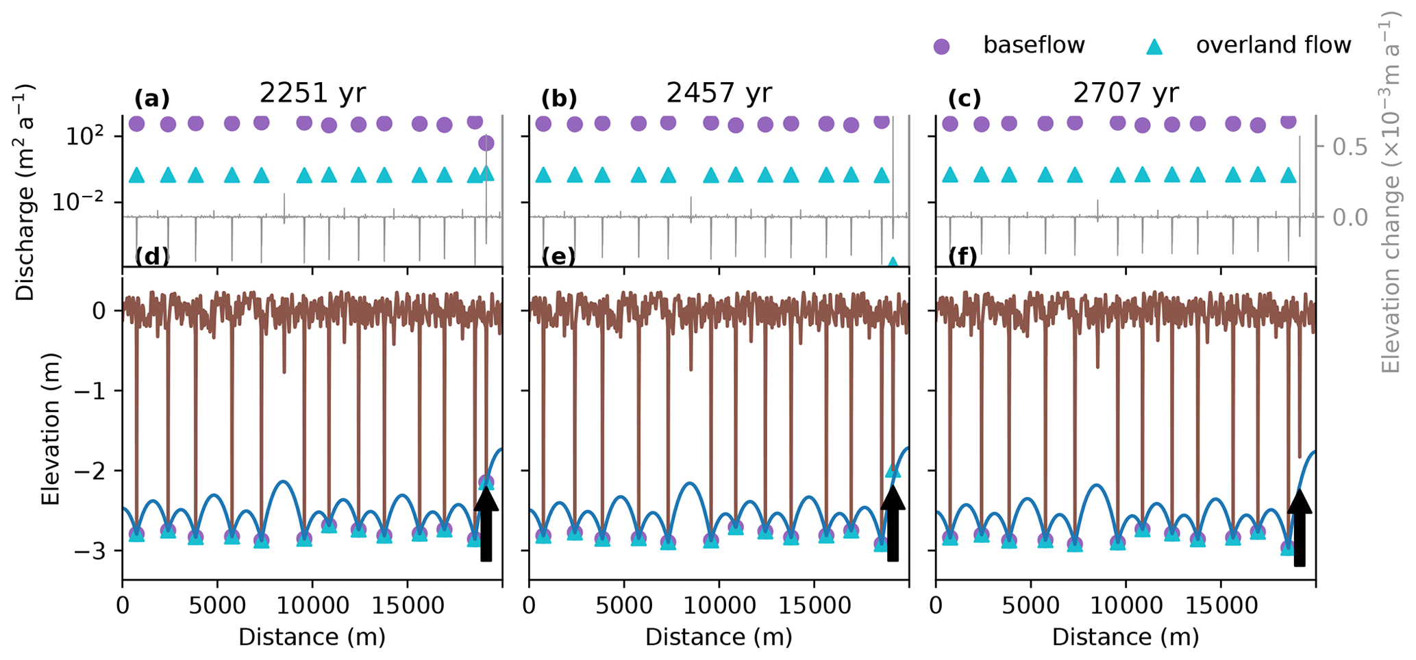
Figure 11 Illustration of groundwater capture in the base-case model run. Panels (a), (b) and (c) show modelled streamflow generated by baseflow and overland flow, and the change in elevation caused by hillslope diffusion and stream erosion for three time slices before, during and after a capture event respectively. Panels (d), (e) and (f) show the modelled position of the land surface and the water table during these three time slices. The arrow points to the stream that loses its connection with the groundwater table.

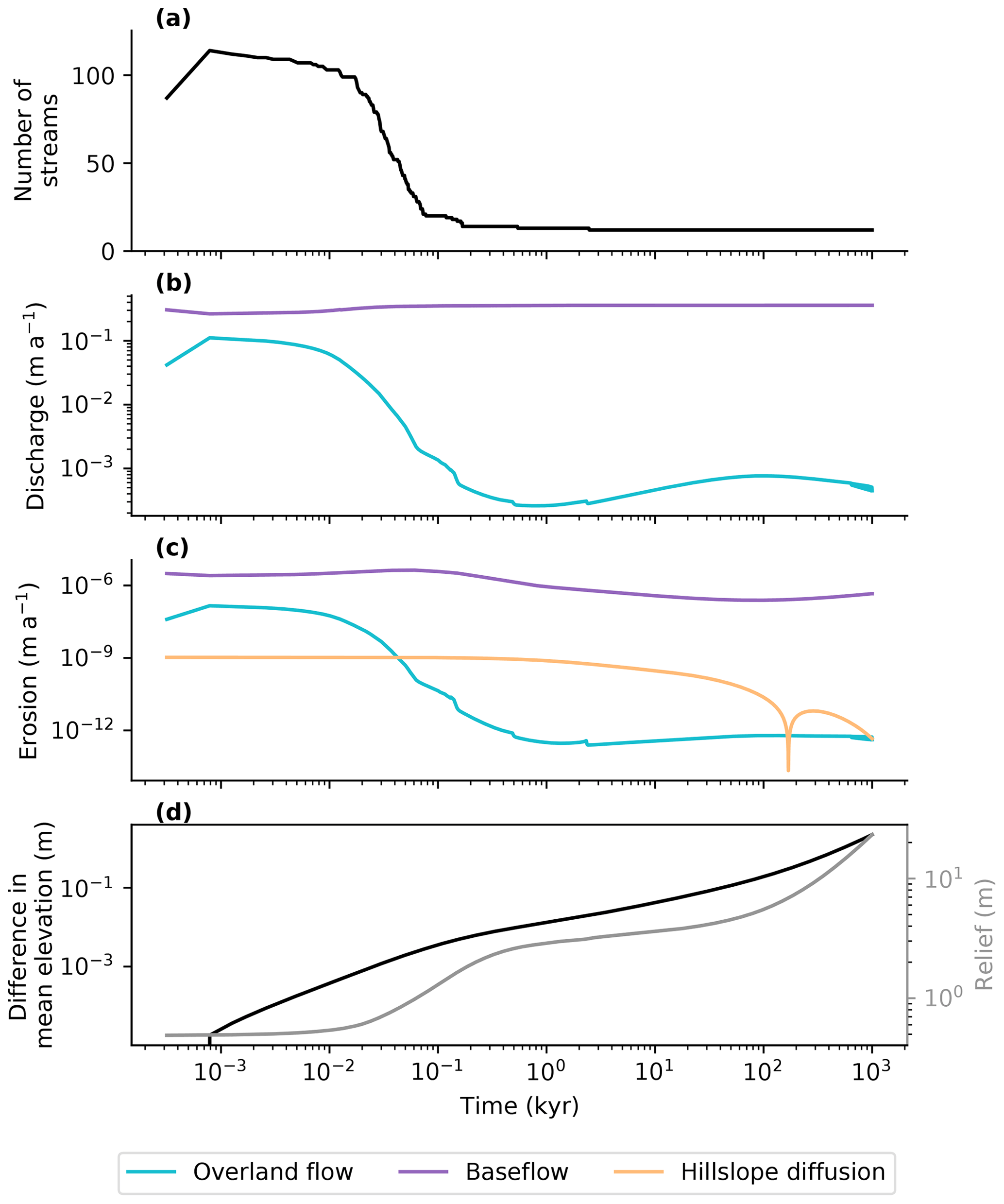
Figure 12 Changes in drainage density (a), water discharge (b), sediment flux (c), and elevation and relief (d) over a time span of 1 million years for the base-case model run. The results show a decrease in active stream channels and a decrease in saturation-excess overland flow over time as streams incise and the water table is drawn deeper below the land surface.

3.2 Sensitivity of drainage density to transmissivity

Groundwater capture is dependent on the transmissivity of the subsurface. This is illustrated by three model runs with different values of transmissivity (Fig. 13). The model run with the lowest transmissivity shows the highest drainage density (Fig. 13a), and the model run with a highest value of transmissivity shows the lowest value of drainage density (Fig. 13c). The reason for this is that low transmissivity results in higher water table gradients, which makes it much more difficult for streams to draw the water table below neighbouring streams and to capture their groundwater discharge. In contrast, high transmissivity results in a relatively flat water table, which means that small differences in incision can already lead to a water table that is drawn below the base of streams. There is a small positive correlation between transmissivity and stream incision rate. The lower number of streams at high values of transmissivity means that these streams receive more water and, therefore, have a higher erosion power. This effect is limited by the negative feedback on stream incision that results from a decrease in stream slope between the modelled cross section and the base level at the downstream (out-of-plane) end of the model domain. For streams with a higher rate of incision, the slope is reduced and their erosional power is decreased.

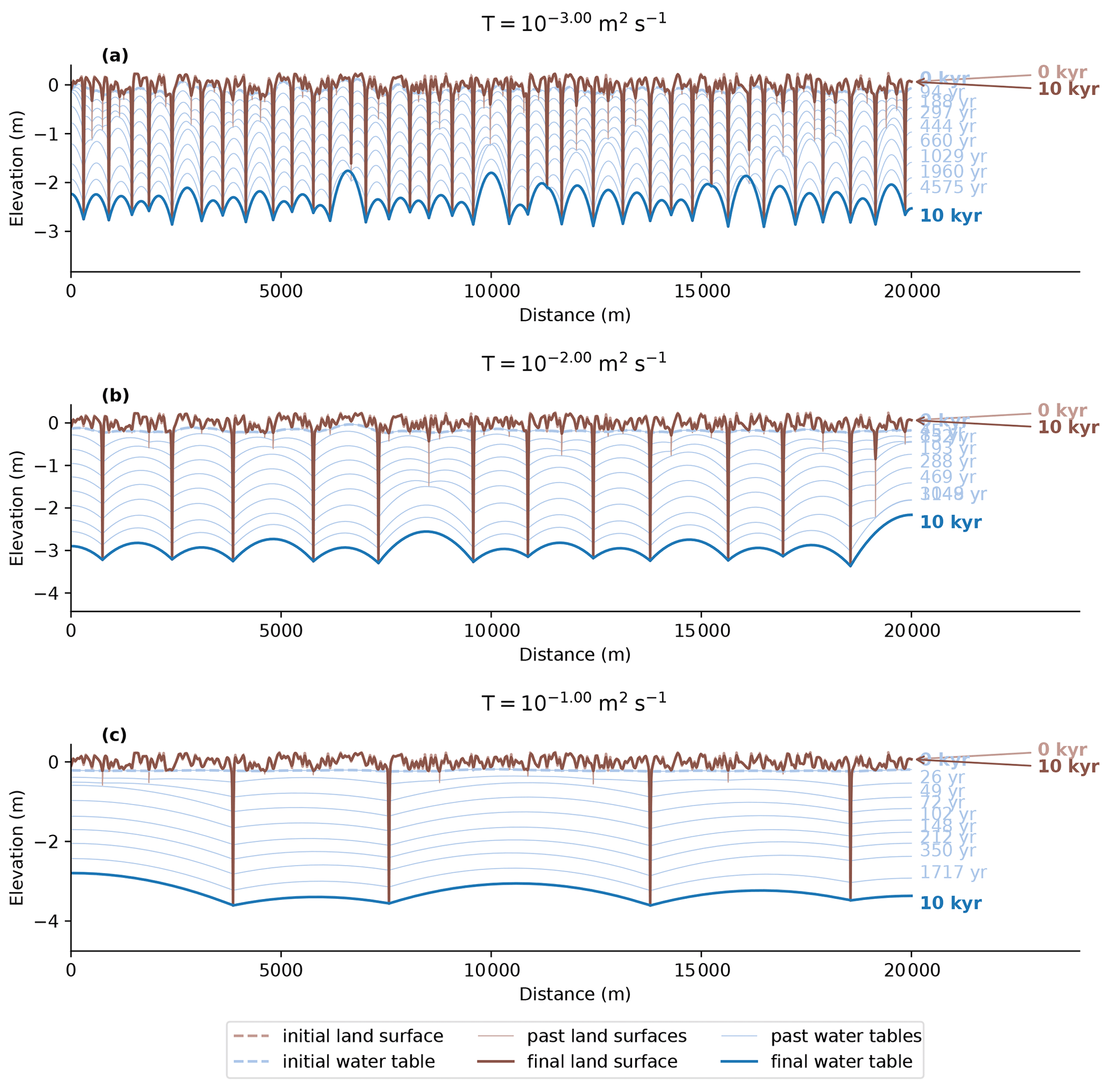
Figure 13 Modelled change in the land surface and water table over time for three model experiments with low ($T={\mathrm{10}}^{-\mathrm{3}}$ m² s⁻¹, panel a), moderate ($T={\mathrm{10}}^{-\mathrm{2}}$ m² s⁻¹, panel b) and high ($T={\mathrm{10}}^{-\mathrm{1}}$ m²s⁻¹, panel c) transmissivity. The results show a negative correlation between drainage density and transmissivity and a positive correlation between transmissivity and stream incision over the model runtime of 10 000 years.

3.3 Sensitivity of drainage density to hydrological and erosion parameters

Comparison of drainage density and incision to a number of parameters that govern erosion and streamflow show that drainage density is the most sensitive to transmissivity and initial slope (Fig. 14). Drainage density is also affected by precipitation and base-level change, whereas it is largely insensitive to specific yield, the sediment transport coefficient and the hillslope diffusion coefficient.

The strong negative correlation of drainage density and initial downstream slope is illustrated in Fig. 15 and can be explained by three effects. First, a higher stream slope means that individual streams have a higher incision power, which means that it is easier to draw the water table below adjacent streams and capture their groundwater discharge. Second, a higher stream slope means a lower base level at the downstream end of the model domain, which means that streams can incise deeper and capture more adjacent streams before the negative feedback kicks in that is associated with deep incision and a reduction in stream slope. Third, a higher initial downstream slope means that more of the total groundwater recharge is directed downstream in the out-of-plane direction, and there is less in-plane groundwater flow (Fig. 3). This results in flatter water tables and an increase in groundwater capture.

Precipitation shows a complex relation with drainage density (Fig. 14), with a positive correlation between drainage density and precipitation at moderate to high values of precipitation, but very high drainage density and low incision rates at low values of precipitation. Precipitation affects groundwater recharge. Given that groundwater flow depends on the ratio of recharge over transmissivity (see Eq. 13), recharge has an effect of equal magnitude to that of transmissivity but is opposite with respect to the direction of the effect; in other words, high precipitation and recharge result in high drainage densities and vice versa. However, at low precipitation values, this trend is reversed, as all recharge contributes to out-of-plane groundwater flow, and the in-plane groundwater flow, baseflow and overland flow rates are too low for the streams to incise. This means that the initially high number of streams does not decrease over time.

Specific yield only has a subtle effect on stream incision. Lower values of specific yield increase the volume of saturation overland flow and make it more difficult for streams to run completely dry, even if they are disconnected from the water table. However, given the subordinate importance of overland flow in generating streamflow and erosion in these model experiments, this effect is very modest and does not change the modelled drainage density or incision rate after a model runtime of 10 000 years (Fig. 14).

The sediment transport coefficient exerts a strong control on the rate of incision and controls how fast the drainage network reaches a steady state. High sediment transport coefficients result in high rates of incision and a relatively fast adjustment of the stream network. However, the rate of incision is ultimately limited by the base level at the downstream end of the model domain, as explained previously; as a result, the sediment transport coefficient only has a minor effect on the modelled drainage density (Fig. 14).

The effect of changes in the hillslope diffusion rate on the development of streams is illustrated in Fig. 16. Although hillslope diffusion may be important in determining drainage density in landscapes with higher relief (Tucker and Bras, 1998; Perron et al., 2008), the incision power of streams is high enough to outpace sediment delivery by hillslope diffusion in this case, and the sensitivity analysis shows no effect of hillslope diffusion on drainage density (Fig. 14). The results do show an effect on the lateral slope of stream valleys and on the rate of infilling of abandoned stream channels (Fig. 16).

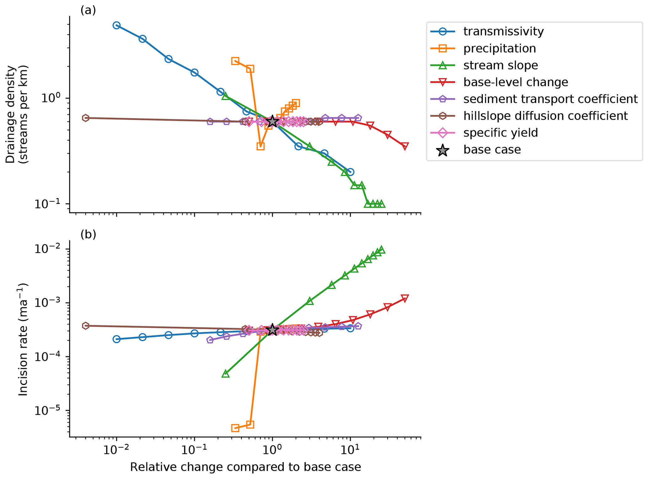
Figure 14 Sensitivity of drainage density and stream incision to hydrological and erosion parameters. The incision rate denotes the incision rate of the stream with the lowest elevation at the end of each model run. Note that the range of parameter values reflects their variability in humid and subhumid settings, as explained in the text.

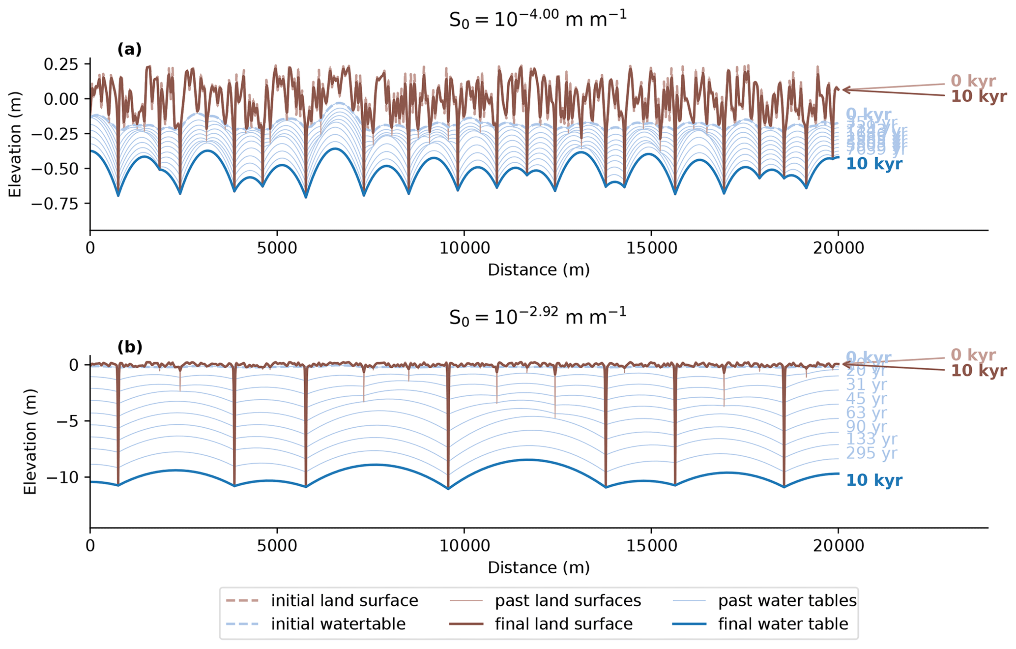
Figure 15 Sensitivity of drainage density and stream incision to initial slope, showing the effects of the lowest (a) and highest (b) slopes that were included in the model sensitivity analysis. Low slopes result in a very low incision power, whereas high slopes provide much more incision power that allows the system to evolve to a situation with fewer active streams. In addition, for low slopes, incision is limited by a relatively high base level at the downstream end of the model domain, whereas for high slopes, the base level is much lower. The base level for the model experiments shown in panels (a) and (b) is located at −2 and −13 m respectively.

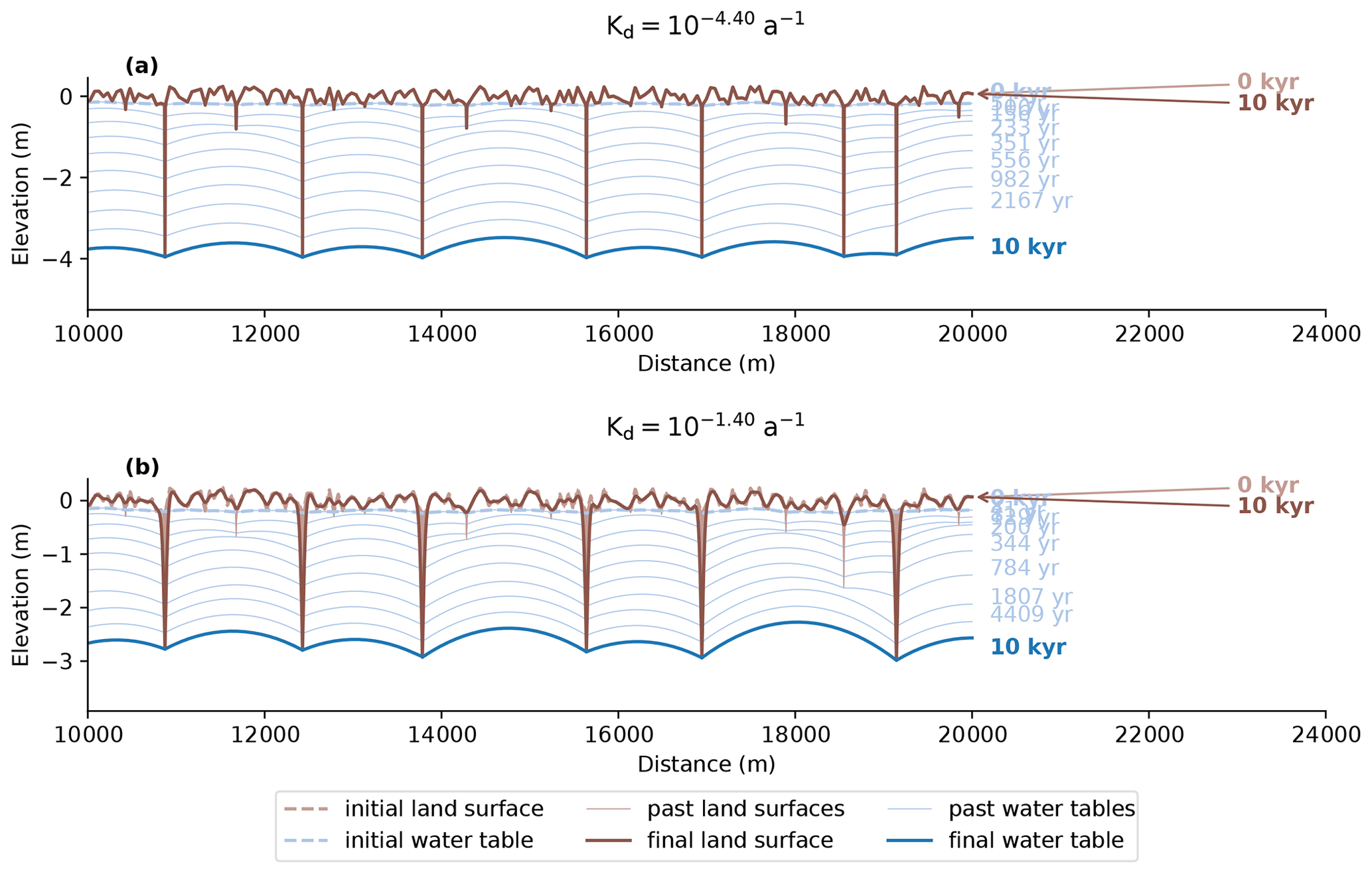
Figure 16 Sensitivity of drainage density and stream incision to hillslope diffusion rate, showing the effects of the lowest (a) and highest (b) hillslope diffusion rates found in a compilation by Richardson et al. (2019). Note that only half of the model domain is shown here to better visualize the effects of hillslope diffusion on valley slope and infill of inactive stream channels.

3.4 The persistence of stream networks

The model runs shown up until this point all started with flat topography with a random perturbation of ±0.5 m. However, the current drainage network in most natural systems started out on an older network that was, for instance, adjusted to glacial conditions during the Pleistocene. The effect of existing incised topography on the modelled adjustment of stream networks is shown in Figs. 17 and 18.

Figures 17 shows the change in the stream network following a change in slope and base level. The results indicate that pre-existing incised topography delays the evolution of stream networks to higher drainage densities, whereas an evolution to lower drainage density proceeds more rapidly. A decrease in slope S₀ from the base-case value of $\mathrm{4}\times {\mathrm{10}}^{-\mathrm{4}}$ to $\mathrm{1}\times {\mathrm{10}}^{-\mathrm{4}}$ m m⁻¹ leads to a decrease in incision over time. However, the effect on drainage density is limited. The drainage density is increased only after approximately 9000 years when the decrease in incision has progressed far enough that the water table reconnects with a previously abandoned stream channel on the right-hand side of the model domain (Fig. 17a). This demonstrates that the stream network shows a degree of delay in adjustment to new conditions that depends on the depth of the water table and the ability of the water table to reconnect with abandoned stream channels or depressions in the landscape. Conversely, an increase in slope leads to an increase in incision that allows the process of drainage capture to proceed (Fig. 17b). Differences in catchment size lead to differences in incision rates and the capture of the groundwater discharge of several small streams by neighbouring streams. This results in a reduction in active streams over time from 12 to 7.

The asymmetry in the response of the drainage network to parameter changes is also shown in the model sensitivity analyses presented in Fig. 18. Compared with model runs that start with a flat topography (Fig. 18a), the model runs that started with an incised topography (Fig. 18b, c) show a comparable response when the parameter change leads to a reduction in drainage density. However, an increase in drainage density is much harder to accomplish, as an increase in drainage density is only possible when the water table is close to the surface. For systems where incision has progressed far enough for the water table to be well below the surface, this requires large changes in precipitation or a large decrease in incision. The adjustment of incision also means that the time that has elapsed since a parameter change is important for drainage density. The delay in adjustment affects models after a runtime of 10 000 years (Fig. 18b) but is much less important for model runs that last 50 000 years (Fig. 18c). The exception is formed by changes in transmissivity, for which the effect is strong enough to generate a fast response in both directions (i.e. for both an increase and decrease in drainage density). However, abrupt changes in transmissivity are probably somewhat unlikely in reality. They could occur for areas with a gain or loss of permafrost (Bogaart et al., 2003), or in the case of the erosion of a confining layer that shields a more permeable layer.

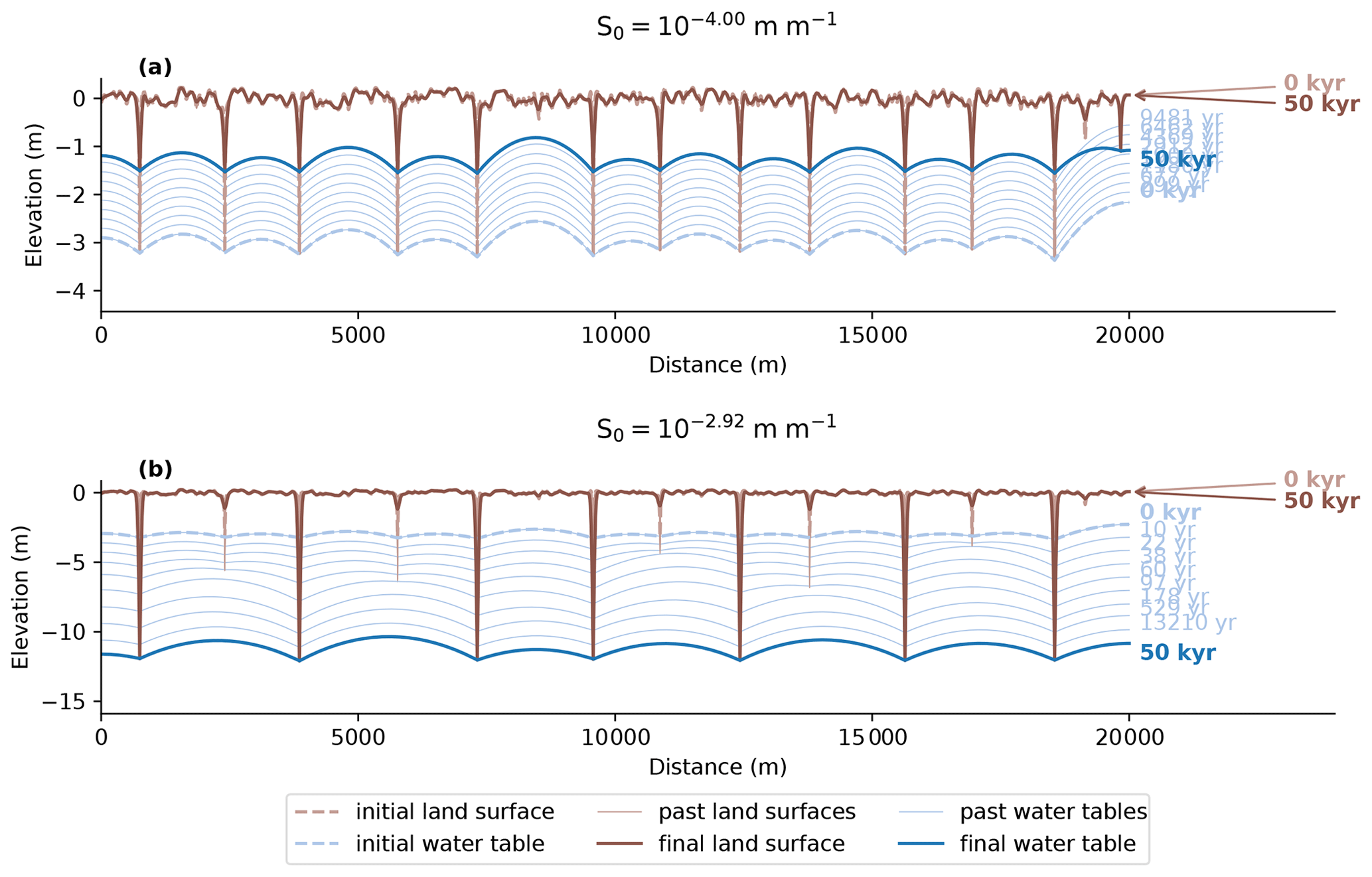
Figure 17 Modelled adjustment of a stream incision for a decrease (a) and increase (b) in slope. The results show that a decrease in slope and the corresponding increase in base level downstream leads to a reduction in stream incision (a) and vice versa (b).

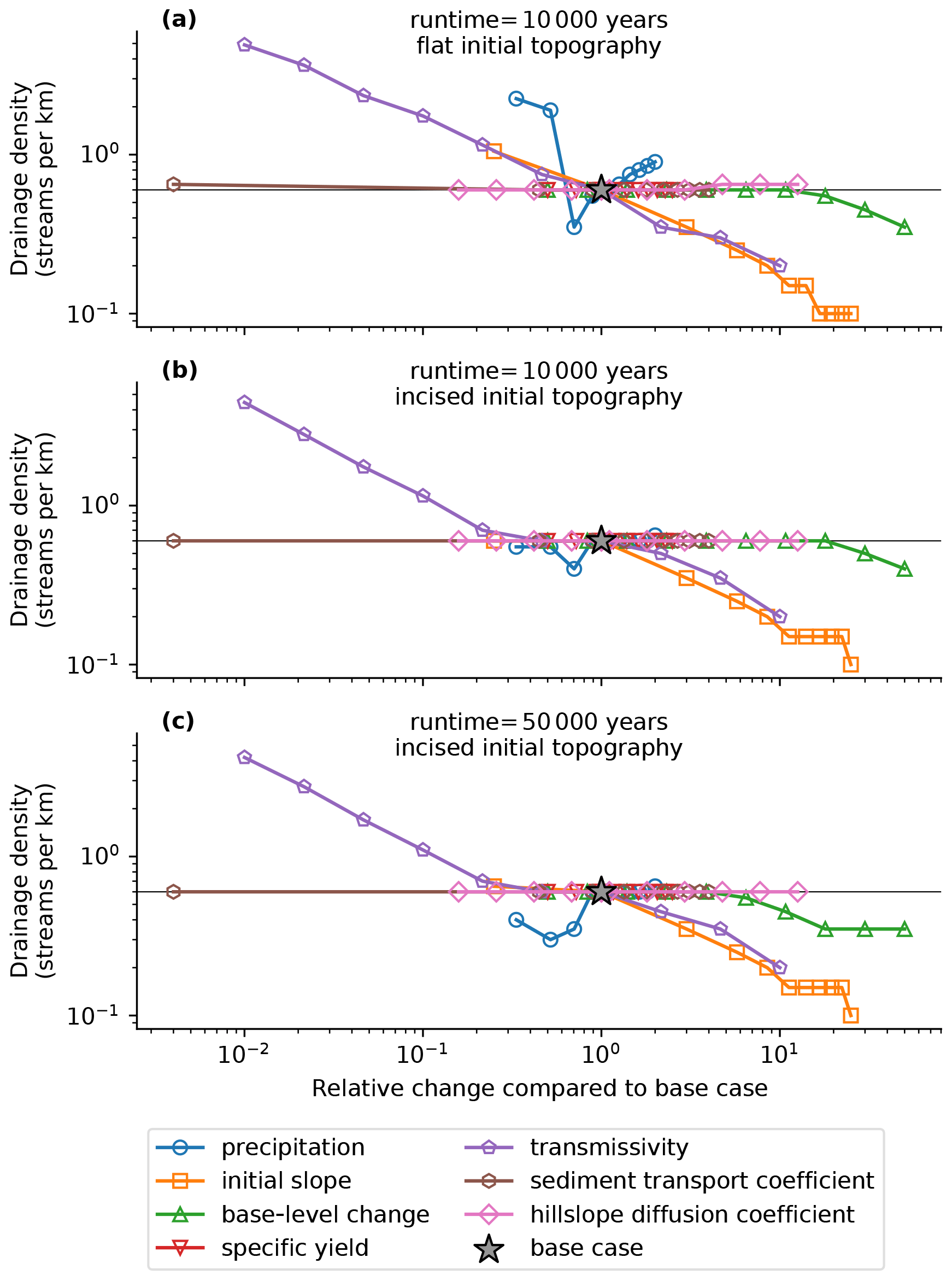
Figure 18 Sensitivity of drainage density to climate, hydrology and transmissivity parameters for different initial topographies and runtimes. Panel (a) shows the sensitivity using a flat initial topography with a perturbation of 0.5 m. Panels (b) and (c) use an incised initial topography, which is equal to the final topography of the base-case model run after a runtime of 10 000 years. For panel (b), the simulation is run for 10 000 years, and for panel (c), the runtime is 50 000 years. The results show that using an incised initial topography reduced the sensitivity of the drainage density to transmissivity and other parameters.

4 Discussion

4.1 Limitations of the model code

The model code presented here was intentionally kept as simple as possible to keep the solutions mathematically tractable and the computational effort manageable. The main limitations are that the model is 2D and only represents a system with perfectly parallel and straight streams; groundwater flow is in a steady state and the contribution of transient groundwater discharge or subsurface storm flow to streamflow is neglected; and the treatment of erosion by overland flow is highly simplified, with an instant addition of all overland flow to the nearest active stream channel as well as a highly simplified distribution of the eroded volume over the length of the channel.

In spite of these limitations, the conclusions of the importance of groundwater flow for drainage density and stream incision are arguably relatively robust. The model results show that groundwater capture is a somewhat inevitable consequence of coupling groundwater flow, streamflow and erosion equations. Regardless of the exact equations and numerical implementation used, the water table will always crop out at perennial streams, and the incision of these streams will draw the water table down. Thus, smaller streams losing their groundwater discharge and eventually falling dry is a logical consequence of differences in incision rate between streams. These conclusions are also supported by previous model studies that found that groundwater flow had a strong effect on erosion (de Vries, 1994; Huang and Niemann, 2006; Barkwith et al., 2015; Zhang et al., 2016) and that a correlation exists between permeability, transmissivity, or lithology and drainage density at a number of locations (Carlston, 1963; Luo and Stepinski, 2008; Bloomfield et al., 2011; Luo et al., 2016).

However, one thing that the model does not represent well is the initiation of stream channels. Due to the 2D nature of the model, the initial topography is represented only in the modelled cross section, and all streams are effectively parallel. This means that, initially, small streams develop in most small depressions. The presence of many small streams divides the water to be discharged over many streams, which each have a very low incision power but are nonetheless considered active streams in the model. In reality, many of these streams would not initiate, as the initial topography would not consist of a set of small depressions that are lined up and connected along an inclined slope. Instead, most of these depressions would be isolated. Therefore, the number of active streams at low runtimes should be much smaller than the high number in the model runs reported here (see e.g. Fig. 12a). In reality, the stream network would develop much more gradually by headward erosion, as shown by natural experiments (Schumm, 1956; Wells et al., 1985; Kashiwaya, 1987; Talling and Sowter, 1999). For the final model results presented in this study, the unrealistic initiation of streams is less of a problem because the stream networks adjust relatively rapidly in the first few 10 to 100 s of years, as stream incision progresses far enough for most of the initial streams to fall dry and for the initial topography to be irrelevant. Therefore, for the final model runtime of a 10 000 years, the unrealistic initiation of stream networks does not affect the results. However, the exception is formed by model runs with low transmissivity ($<{\mathrm{10}}^{-\mathrm{4}}$ m² s⁻¹) or low initial slope ($<{\mathrm{10}}^{-\mathrm{4}}$ m m⁻¹), for which the ability to capture groundwater discharge and the incision power of the streams is too low to escape the initial phase with a dense stream network.

4.2 Groundwater capture

To my knowledge, the process of groundwater capture that is illustrated here has not been proposed before. Studies by de Vries (1976) and de Vries (1994) discussed the opposite process, in which new streams establish themselves when the water table reaches the land surface following an increase in precipitation and groundwater recharge. Twidale (2004) suggested that stream incision may induce a positive feedback by increasing groundwater flow and runoff to streams that incise faster, although the study did not provide any further details.

The process of groundwater capture is expected to be important wherever streamflow is dominated by either groundwater discharge or saturation overland flow. In systems where infiltration-excess flow is dominant, which include most semi-arid and arid regions (Kidron, 2021), groundwater capture could still occur and would determine which streams discharge groundwater and are active perennially, but streams that are detached from the groundwater table would still be able to incise. In addition, groundwater capture may be less important for systems dominated by subsurface storm flow in perched aquifers that are detached from the water table. However, the importance of this flow mechanism is uncertain and is still under debate (Freeze, 1972; Chifflard et al., 2019).

Note that the difference between the groundwater capture process and the more well-studied process of stream capture (Whipple et al., 2017) is that groundwater capture does not require a physical connection between two streams and may, therefore, not leave a clear trace in the landscape, as opposed to river capture. The capture of the groundwater discharge of one stream by another results in the first stream becoming dry, but the hillslope between these streams remains intact, as can be seen in Fig. 11.

4.3 Comparison with field studies

The model study presented here used climate, hydrology and erosion parameters that were based on the southern Netherlands (de Vries, 1994; Bogaart et al., 2003). The model results match the observed drainage density and rate of incision in the southern Netherlands relatively well. The modelled drainage density after a runtime of 10 000 years is 0.6 streams per kilometre, which is close to the observed average drainage density of approximately 0.5 streams per kilometre (de Vries, 1994, 1995). In addition, the incision of approximately 3 m is also close to the values observed in the southern Netherlands. This means that the model was able to reproduce the current drainage network that likely developed in response to climate and base-level changes after the end of the Pleistocene (de Vries, 1994; Bogaart et al., 2003).

The negative correlation between transmissivity and drainage density that the model results shows (Fig. 13) has been discussed previously in the literature. Carlston (1963) used theoretical considerations to deduce that high transmissivity leads to high rates of baseflow and low rates of direct surface runoff. A compilation of 13 catchments in the eastern USA with similar climate and recharge found a negative linear correlation between baseflow and the square root of drainage density. When assuming that baseflow and transmissivity are correlated linearly, this also results in a negative correlation between the square root of drainage density and transmissivity.

Figure 19 contains a compilation of quantitative data on transmissivity and drainage density along with the model results presented in this study. The data compilation supports a negative correlation between drainage density and transmissivity. Previous work by Bloomfield et al. (2011) found a significant correlation between drainage density and hydraulic conductivity for nine catchments in the Thames Basin, UK. In addition, parts of the Oregon Cascades covered by Tertiary and Quaternary rocks showed a remarkable contrast in drainage density and incision that correlates with a difference in hydraulic conductivity and transmissivity (Luo and Stepinski, 2008; Luo et al., 2010).

Although the field data show the same trend as the model results, the predicted drainage densities for low transmissivities ($<{\mathrm{10}}^{-\mathrm{3}}$ m² s⁻¹) in the model sensitivity analysis are much higher than in the Bloomfield et al. (2011), Luo and Stepinski (2008) and Luo et al. (2010) datasets (Fig. 19). The reason for the difference is likely the relatively low initial slopes and the relatively high base level in the model runs that mimic the low relief in the southern Netherlands. Low relief and high base level limit groundwater capture and lead to high drainage density, as shown by the model sensitivity analysis (Fig. 14). In addition, most of the catchments in the Bloomfield et al. (2011) dataset and the Cascades are bedrock catchments with very different erosion parameters compared with the unconsolidated sediments in the southern Netherlands. Note that the transmissivity values for the Bloomfield et al. (2011), Luo and Stepinski (2008) and Luo et al. (2010) datasets shown in Fig. 19 are relatively uncertain. Transmissivity was estimated from reported hydraulic conductivity values using an estimated aquifer thickness of 100 m. The hydraulic conductivity values in the Bloomfield et al. (2011) dataset are partly based on grey literature and analogies with lithological units elsewhere. The values reported by Luo and Stepinski (2008) and Luo et al. (2010) are based on a method where the water table is assumed to be at the surface at groundwater divides. This is not likely to be true in all cases; therefore, these values should be considered minimum estimates.

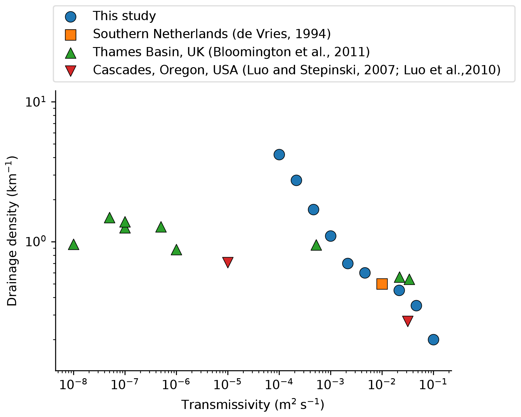
Figure 19 Comparison of the modelled relation between transmissivity and drainage density with field observations (Bloomfield et al., 2011; Luo and Stepinski, 2008; Luo et al., 2010; de Vries, 1994). The reported hydraulic conductivity values from Bloomfield et al. (2011), Luo and Stepinski (2008), and Luo et al. (2010) were converted to transmissivity via multiplication by an estimated aquifer thickness of 100 m. The model results and the field data both show a negative correlation between drainage density and transmissivity. The difference in magnitude is probably related to differences in relief and geology.

4.4 Implications for landscape evolution modelling

The strong correlation between drainage density, transmissivity and groundwater flow shown in both the model results and field data means that the inclusion of groundwater flow and a representation of the water table could strongly improve models of stream network evolution, landscape evolution, and water and sediment fluxes over geological ($>\approx {\mathrm{10}}^{\mathrm{4}}$ a) timescales. The approach shown in this study relies on a partitioning of rainfall into overland flow and groundwater flow, with groundwater flow assumed to be at steady state. The advantages of modelling steady-state, depth-integrated groundwater flow are the simplicity and low computational demands. The exchange between groundwater and surface water was modelled using a seepage algorithm. Similar seepage or drainage algorithms are also able to efficiently couple surface water and groundwater flow in depth-integrated 2D or full 3D models of groundwater flow (Batelaan and De Smedt, 2004) and would, therefore, be readily available for integration with existing landscape evolution model codes. The assumption of steady-state groundwater flow used in this study is a simplification that omits the effects of transient groundwater discharge. Transient groundwater discharge may be important to include in landscape models, as transient peak groundwater flow rates to streams may have a large effect on erosion. However, 3D models of coupled transient groundwater and surface water flow tend to be computationally demanding and often require parallel computing architectures (Kuffour et al., 2020), which limits the possibility to explore parameter space and model sensitivity. Simplified descriptions of transient groundwater flow similar to the new equation for the integrated discharge and erosion by overland flow events (Sects. 2.6.4 and 2.7.3) could be developed and added to landscape model codes. Such an approach could help constrain the importance of transient groundwater flow for stream incision for different hydrological parameters and different geographic settings.

In addition to being potentially beneficial for models of landscape evolution, a tighter integration of landscape evolution and groundwater models could also improve knowledge of groundwater and surface water systems. The groundwater table is often assumed to follow the topography to some degree, and groundwater divides are often assumed to coincide with surface water divides (Liu et al., 2020). However, the validity of this assumption in different geological settings is uncertain. Integrated landscape and groundwater flow models could help quantify the extent to which the water table can be expected to follow topography and the extent to which surface water divides and groundwater divides are expected to coincide.

5 Conclusions

A new model is presented that couples equations that govern groundwater flow, overland flow, streamflow and erosion and that represents humid regions where infiltration-excess overland flow is negligible. The coupling of these equations reveals a strong dependence of drainage density on groundwater flow and transmissivity. The dependence of drainage density on groundwater flow is controlled by a process identified here as groundwater capture, whereby faster incising streams draw the water table below neighbouring streams, which become dry and lose the ability to incise any further. This process is more efficient when the water table is relatively flat, which can be due to either low groundwater recharge or high transmissivity, with transmissivity often being the dominant control due to its high variability. Sensitivity analysis shows that the importance of transmissivity for drainage density is roughly equal to the base level and initial slope and exceeds other hydrological and erosion parameters such as precipitation and the hillslope diffusion coefficient. These results agree with published field data from the Thames Basin, UK, and the Cascades, USA, that show a negative correlation between transmissivity and drainage density. The results also imply that groundwater and transmissivity may be a dominant control on drainage density in humid regions. Landscape evolution models may need to include groundwater flow and the water table. At the same time a closer integration of landscape and groundwater data and models may help improve knowledge of the evolution of the Earth's surface.