the Creative Commons Attribution 4.0 License.
the Creative Commons Attribution 4.0 License.
 | 09 Dec 2022
Combining seismic signal dynamic inversion and numerical modeling improves landslide process reconstruction
Yifei Cui
Xinghui Huang
Jiaojiao Zhou
Wengang Zhang
Shuyao Yin
Landslides present a significant hazard for humans, but continuous landslide monitoring is not yet possible due to their unpredictability. In recent years, numerical simulation and seismic inversion methods have been used to provide valuable data for understanding the entire process of landslide movement. However, each method has shortcomings. Dynamic inversion based on long-period seismic signals gives the force–time history of a landslide using an empirical Green's function but lacks detailed flowing characteristics for the hazards. Numerical simulation can simulate the entire movement process, but results are strongly influenced by the choice of modeling parameters. Therefore, developing a method for combining those two techniques has become a focus for research in recent years. In this study, we develop such a protocol based on analysis of the 2018 Baige landslide in China. Seismic signal inversion results are used to constrain and optimize the numerical simulation. We apply the procedure to the Baige event and, combined with a field geological survey, show it provides a comprehensive and accurate method for dynamic process reconstruction. We found that the Baige landslide was triggered by detachment of the weathered layer, with severe top fault segmentation. The landslide process comprised four stages: initiation, main slip, blocking, and deposition. Multi-method mutual verification effectively reduces the inherent drawbacks of each method, and multi-method joint analysis improves the rationality and reliability of the results. The approach outlined in this study could help us to better understand the landslide dynamic process.
- Article
(17447 KB) - Full-text XML
-
Supplement
(1567 KB) - BibTeX
- EndNote


Landslides present a significant hazard for humans; the number of fatalities resulting from non-coseismic landslides between 2004 and 2016 averaged 4000 per year (Froude and Petley, 2018). However, they cannot be continuously monitored due to their unpredictability and the difficulty of their detection (Chen et al., 2013; Yamada et al., 2013; Feng et al., 2016; L. Wang et al., 2020), and the landslide movement process cannot be fully understood through post-event field investigation and remote sensing alone. Hence, to aid warning and prevention of landslide hazards and reduce associated losses, there is an urgent need to develop alternative methods to enable in-depth investigation of the dynamic characteristics of landslide generation and movement.
Landslide movement generates seismic signals that propagate to the surrounding area. The development of environmental seismology and construction of global seismic networks (Dammeier et al., 2016) means the seismic signals generated by landslide movement can be quantitatively recorded by nearby seismic stations (Walter et al., 2012; Yamada et al., 2012, 2013; Chen et al., 2013). Seismic signals generated by landslides reflect the duration, location, and scale of the event (Kao et al., 2012; Yamada et al., 2012; Chen et al., 2013); seismic signal analysis is increasingly used for landslide hazard monitoring and early warning, but it also offers a research tool for understanding landslide dynamics. The size and location of landslides can be estimated from the amplitude, frequency range, and time–frequency spectrum of the seismic signal (Favreau et al., 2010; Moretti et al., 2012, 2015), along with timing of the event (Sakals et al., 2011; Zhang et al., 2019) and landslide dynamics (Yamada et al., 2013; Hibert et al., 2015; Jiang et al., 2016). The method of detecting, locating, and identifying landslide events using broadband seismograph records is based on associating seismic signals with landslide characteristics. Some progress has been made in interpreting landslide seismic signals, but signal recognition is often hindered by interference from seismic signals generated by other factors (Feng, 2011; Zhao et al., 2015; Fuchs et al., 2018). Several methods have been developed to solve signal noise pollution (Helmstetter and Garambois, 2010; Feng, 2011), but analysis of landslide dynamic characteristics and reconstruction of landslide processes is still subject to errors and inaccuracies. Recently, filtering of seismic signals has been successfully applied to reconstruct dynamic landslide processes, allowing transition stages to be identified that are difficult to derive from field analysis alone (Yan et al., 2020a, b).
Combining seismic signal analysis with dynamic inversion can improve the extraction of landslide dynamic characteristics. Landslide dynamic inversion using long-period seismic records based on a single-force source model (Kanamori and Given, 1982; Kanamori et al., 1984; Hasegawa and Kanamori, 1987; Dahlen, 1993; Fukao, 1995) and a static point source assumption has been widely adopted to study landslide kinematics (Allstadt, 2013; Ekström and Stark, 2013; Yamada et al., 2013; Hibert et al., 2014, 2015; Moore et al., 2017; Gualtieri and Ekström, 2018; W. Li et al., 2019; Sheng et al., 2020; Zhao et al., 2020). Predictive relationships between the maximum inverted forces and sliding volume can be derived from inverted landslide force histories (Ekström and Stark, 2013; Chao et al., 2016). Landslide basal friction is estimated directly using a block model (Brodsky et al., 2003; Allstadt, 2013; Yamada et al., 2013; Zhao et al., 2015; Yu et al., 2020) or obtained from seismic analysis coupled with numerical simulation (Moretti et al., 2012, 2015; Yamada et al., 2016, 2018). Although numerical simulation of landslide dynamic processes has achieved remarkable results, there are issues with each of the following three main approaches. The continuous medium approach, including smoothed particle hydrodynamics (SPH) (Pastor et al., 2014), the material point method (MPM) (Soga et al., 2016), the finite-element method (FEM) (Muceku et al., 2016), the finite-volume method (FVM) (Pitman et al., 2003), and the finite-difference method (FDM) (Shen et al., 2020), is not very effective in describing particle separation and internal fracture of rockslides. The thin-layer models are based on the thin-layer approximation and depth-averaging process of the Navier–Stokes equations without viscosity, but a main issue is low computational accuracy (Moretti et al., 2012, 2015; Yamada et al., 2016, 2018). The discrete-element approach utilizes software such as particle flow code (PFC) (Lo et al., 2011; S. L. Zhang et al., 2020) and discrete-element method solutions (EDEM) (W. Wang et al., 2020), but a major issue is low computational efficiency. MatDEM uses an innovative matrix discrete-element method and three-dimensional contact algorithm, which can realize the efficient numerical simulation of millions of particles (Liu et al., 2013, 2017). However, studies utilizing MatDEM mostly determine the correctness of landslide simulation through comparison with post-event landslide characteristics derived from field investigation (Liu et al., 2017), which may not represent dynamic processes. An alternative approach that offers potential is to use seismic signal inversion as the constraint on landslide dynamic process (Yamada et al., 2016, 2018).
In this study, we use long-period seismic signals to obtain the dynamic characteristics of Baige landslide, China, which occurred on 10 October 2018 (termed the “10.10.” event). Combined with the inversion results, the landslide process was reconstructed by numerical simulation. Through seismic signal analysis, landslide dynamic inversion, and numerical simulation, combined with the post-event field investigation, we try to provide an improved characterization of the landslide movement process.
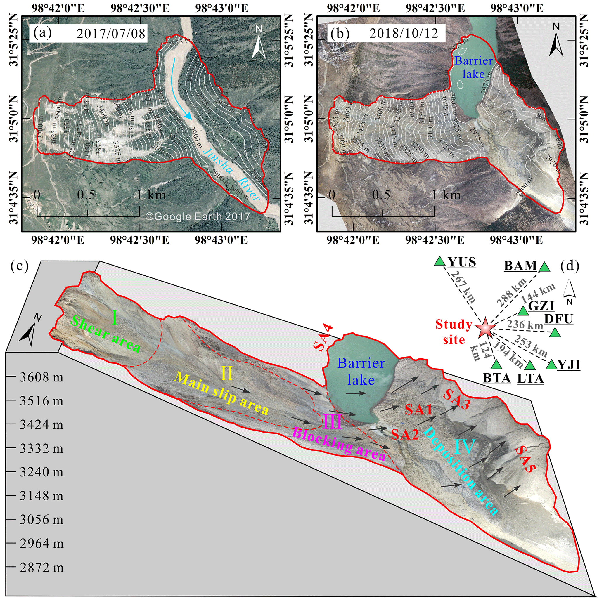
Figure 1Location of the study area. (a) Digital orthophoto map (DOM) of the Baige landslide area in 2017, (b) DOM of Baige landslide after the 2018 event, (c) schematic cross section with remote sensing overlay showing key features of the Baige landslide (SA1 and SA2 are the two main accumulation zones, the debris of SA1 is mainly from the shear area, while that of SA2 is mainly from the main slip area and blocking area; SA3 is the left bank of the river, scoured by landslide debris; SA4 is a small area of the right bank scoured by landslide debris; SA5 is the downstream left bank, which is affected by the landslide body mix with the sandblasting water), and (d) location of the Baige landslide (red star) relative to seismic stations (green triangles) used in the study. The remote sensing image map data of (a) is from the © Google Earth 2017, and the data of (b) and (c) are from the authors' own uncrewed aerial vehicle (UAV) photography measurements.
A massive landslide occurred at Baige, on the eastern Qinghai–Tibetan Plateau, China on 10 October 2018 (termed as the 10.10. event) (Fig. 1). The landslide caused the blockage of the main stream of Jinsha River and formed a barrier lake. On 12 October, the water of the barrier lake began to discharge naturally until the discharge was completed on 13 October (Liu et al., 2021). On 3 November 2018, the rock and soil mass at the trailing edge of the slide source area of the first Baige landslide was unstable again, causing the second landslide. It has been studied by many researchers, Xu et al. (2018), Deng et al. (2019) and Fan et al. (2019b) analyzed the formation mechanism and process of the landslide and found that the site is in the Jinsha River suture zone, where the influence of multiple tectonic movements provides a complicated regional tectonic profile; the main fault structures trend NW, within the Jiangda–Bolo–Jinshajiang fault zone (Fig. 2). Ouyang et al. (2019), Fan et al. (2019a), and W. Wang et al. (2020) carried out numerical simulation analysis of the Baige landslide. In this study, only the 10.10. Baige landslide was studied. The landslide can be divided into four areas, namely, shear, main slip, blocking, and deposition, with maximum and average thicknesses of 80 and 50 m (Fig. 1c). We used terrain data from Ouyang et al. (2019), comprising a 10 m resolution pre-landslide digital elevation model (DEM) from 2017, and a 5 m resolution post-slide DEM obtained through uncrewed aerial vehicle (UAV) photogrammetry in 2018 from field investigation. Based on DEM differencing, total landslide volume was calculated as 1.96×10⁷ m3. The altitude range of the initiation zone is 3523 to 3730 m. Most of the rock mass that collapsed from the steep back wall accumulated at an elevation of 3100 to 3300 m in an area of gentle slope angle from 20 to 25∘.
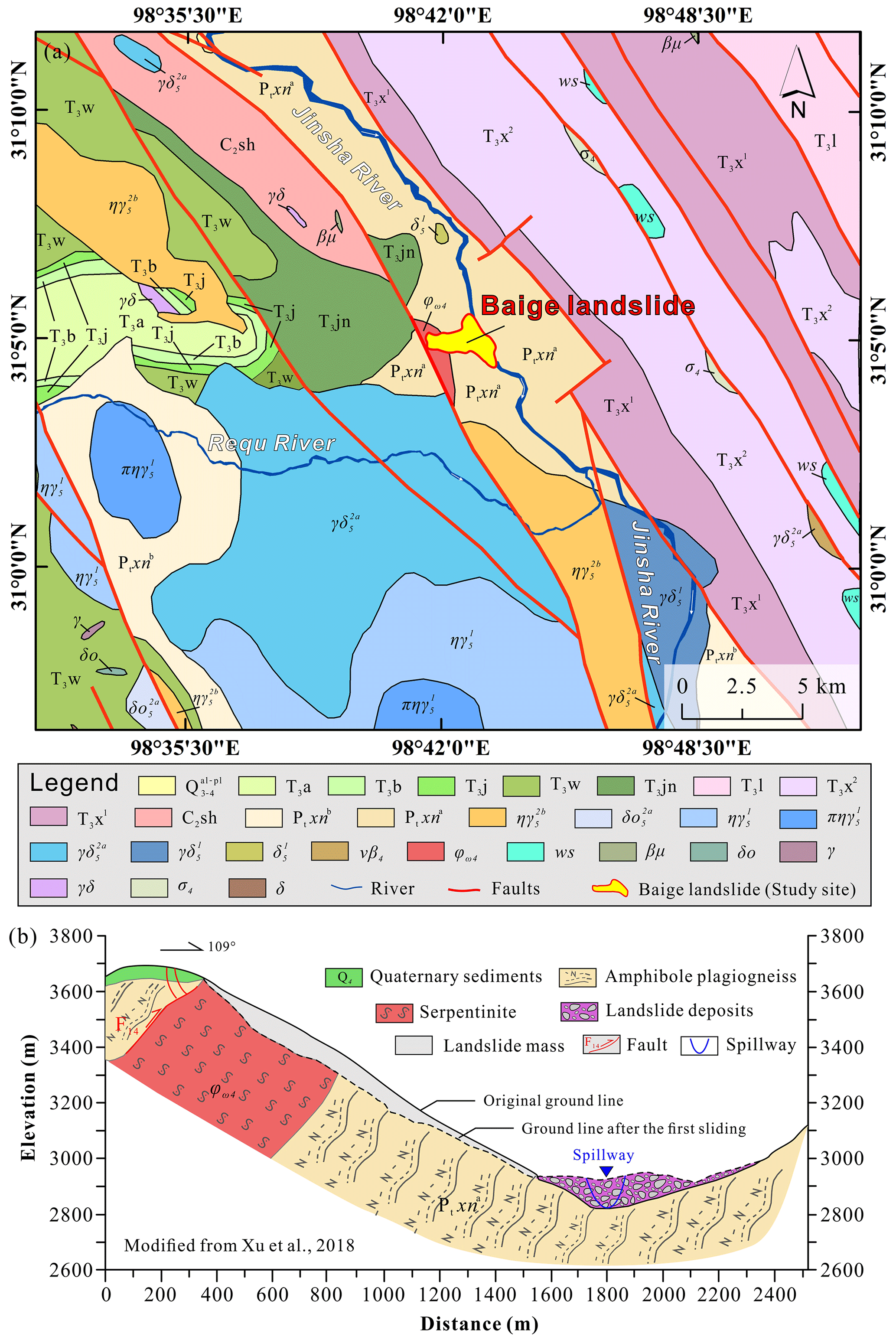
Figure 2Geology of the study area. (a) Geological map of the Baige landslide area (: Quaternary Holocene–Upper Pleistocene; T3a, T3b, T3j, T3w, T3jn, T3l, T3x2, T3x1: Upper Triassic; C2sh: Upper Carboniferous; Ptxnb, Ptxna: Proterozoic; , : Yanshan period; , , , , : Indosinian; vβ4, ϕω4, σ4: Variscan; ws: detached block; βμ: diabase–porphyrite; δo: quartz diorite veins; γ: granite veins; γδ: granodiorite dikes; δ: diorite veins). (b) Cross section of the landslide showing the geological profile. The geological map data in (a) is from C. Y. Li et al. (2019), and the cross section in (b) is modified from Xu et al. (2018).

Figure 3Probabilistic power spectral density of the vertical component at seismic station BTA. Red line in the PSD image is NHNM and green line is NLNM. Below the PSD image is a visualization of the data basis for the calculation. The top row shows data fed into the calculation, with green patches representing available data. The bottom row in blue shows the single PSD measurements that go into the histogram.
We selected broadband seismic signals from seven seismic stations that are distributed around the landslide with adequate azimuth coverage (Fig. 1d) to carry out the analysis. Landslide force history inversion uses long-period seismic waveforms and thus requires that the ambient noise at periods of tens of seconds should be at a low level in the study area. We used the probabilistic power spectral density (PSD) technique (McNamara and Buland, 2004) to characterize the background seismic noise. As illustrated by the PSD of the vertical component for seismic station BTA (Fig. 3), the main seismic energy is distributed between the new high-noise model (NHNM) and the new low-noise model (NLNM) (Peterson, 1993), indicating that the study area has a relatively good seismic observation environment. Before carrying out the dynamic inversion, we will calculate the signal-to-noise ratio (SNR) for each seismic trace and use it to determine if the trace will be used in the inversion, about which a detailed description can be found in Sect. 4.2.
3.1 Seismic data analysis
We used short-time Fourier transform (STFT) and PSD to quantitatively analyze the seismic signals for Baige landslide (Yan et al., 2020a, b). A time–frequency domain transform of the seismic signal using STFT allowed information on both the time and frequency domain distributions of the seismic signal to be obtained. The power of each unit of frequency for each frequency band component that corresponds to a specific moment was estimated based on the PSD of the seismic signal in the frequency domain.
3.2 Landslide force history inversion
Assuming the landslide source is represented as a series of time-varying forces acting on a static point, synthetic seismograms un(x,t) at the seismic station located at x can be computed by convolution of force fi(x0,t0) at x0 with nine-component Green's functions (Moretti et al., 2012; Allstadt, 2013; Ekström and Stark, 2013; Yamada et al., 2013; Hibert et al., 2014; Li et al., 2017; Gualtieri and Ekström, 2018),
where ∗ denotes convolution and bold typeface indicates a vector. The Einstein summation convention is assumed in the equation. The convolution can be rewritten as matrix product,
Suppose there are N seismic traces,
using , and , we get the linear forward model
We use uo to denote observed seismic records and define the two-norm of the vector difference between uo and u as an objective function,
An optimal solution of the forces can be obtained in a least-squares sense,
The landslide force history can be reconstructed by direct deconvolution of the observed seismograms with Green's functions, which can be readily performed in both time and frequency domains (Allstadt, 2013; Yamada et al., 2013; Li et al., 2017). We calculated Green's function at the landslide location for each seismic station using a matrix propagation method (Wang, 1999) and a 1-D layered velocity model from Crust1.0 (https://igppweb.ucsd.edu/~gabi/crust1.html, last access: 10 October 2021).
Once the landslide force history f was inverted, based on Newton's third law of motion, the forces acting on the sliding mass could be obtained by multiplying the inverted force history by −1 (Kanamori and Given, 1982; Yamada et al., 2013; Gualtieri and Ekström, 2018). The forces acting on the sliding mass can then be used to calculate its velocity and displacement distributions for a given mass (Z. Li et al., 2019; Yu et al., 2020) or to estimate the sliding mass by minimizing discrepancies with independently derived sliding trajectories (Hibert et al., 2014) using the following equations,
3.3 Numerical modeling
3.3.1 Discrete-element method
To quantitatively analyze the process of landslide initiation, movement, and accumulation for the 10.10. Baige event, we used MatDEM software, which is based on the matrix discrete-element method, to numerically simulate the landslide (Liu et al., 2017). The discrete-element method has been widely used in simulation of geological hazards (An et al., 2021; Cui et al., 2022; Fang et al., 2022). In this method, particle movement obeys Newton's second law, and particle velocity and displacement are sequentially updated to simulate the dynamic process of the landslide. In MatDEM, the landslide body is formed by the accumulation and cementation of particles endowed with specific mechanical properties, and the contacts and interactions of these particles are defined by the linear elastic bonded model, as shown in Fig. 4a. The normal force Fn and tangential force Fs between particles can be expressed by the following formulae:
where Kn is the normal stiffness, Xn is the normal relative displacement between two particles at the contact point, Ks is the tangential stiffness, and Xs is the tangential displacement.
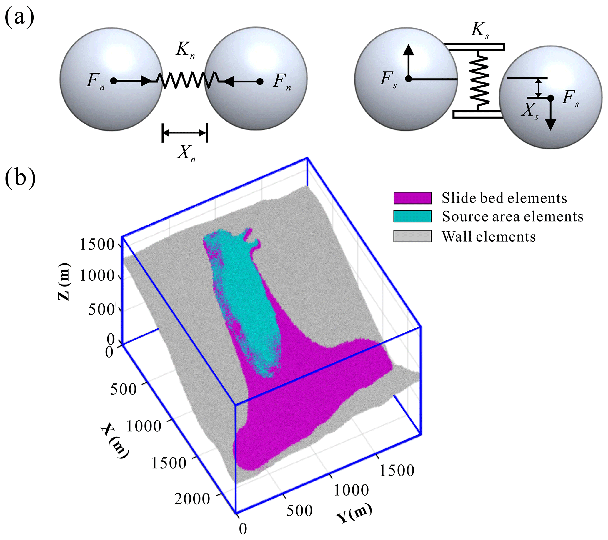
Figure 4Schematics showing properties of landslide particles and discrete-element model. (a) Linear elastic bonded model. (b) Discrete-element model of the Baige landslide (Fan et al., 2019a).
In the normal direction, when the displacement between particles Xn exceeds the fracture displacement Xb, the connection between particles is broken and the tension is set as zero. In the tangential direction, spring failure follows the Mohr–Coulomb criterion, and the tangential bond is broken when tangential force exceeds maximum shear force , meaning that only sliding friction (−μpFn) exists between particles −μpFn. The maximum normal force and maximum tangential force that the cementation between particles can withstand is
where is the shear resistance between particles and μp is the friction coefficient between particles.
3.3.2 Discrete-element model of Baige landslide
In MatDEM, the base of the landslide model is constructed of densely packed particles (20 m thick) arranged according to the topography of the slope base. The coordinates of these particles are fixed in the simulation (gray particles in Fig. 4b). The landslide area is constructed by particles accumulated in the cube model box using cutting topography of the pre- and post-landslide. Before starting the simulation, gravity is applied to particles in the sliding source area (blue particles in Fig. 4b) and sedimentary layer (20–80 m thick) (purple particles in Fig. 4b); breaking the connection between particles in the source area allows them to slide down under the action of gravity to simulate landslide initiation. We used a simulation block of m, with 582 000 particles comprising 169 000 active cells for simulating landslide movement and 413 000 boundary elements to fill the geometry (bottom) and limit the range of activity (side). Average cell size was 5 m and the real-world time 80 s.
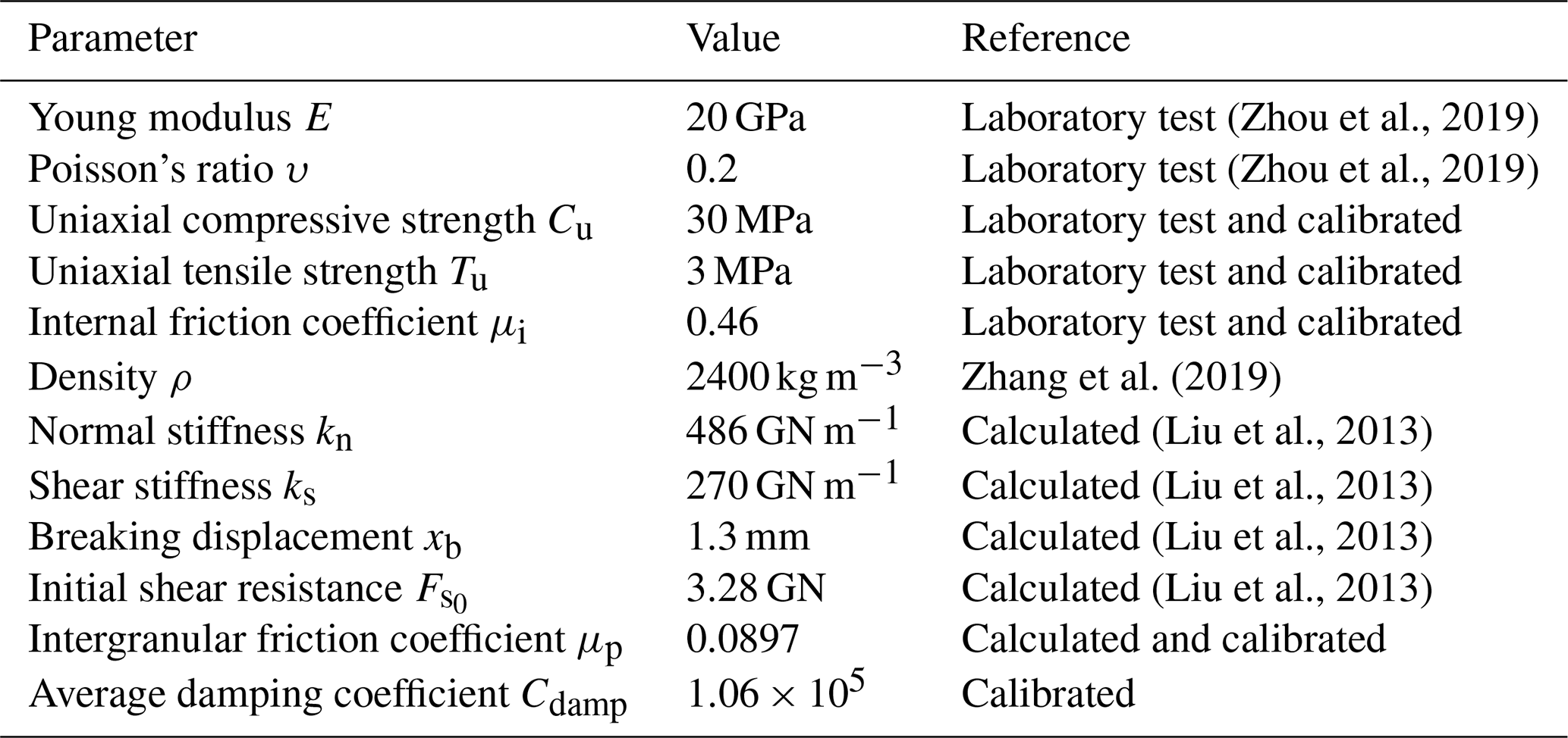
As shown in the flow chart of Fig. 5, we used the dynamic inverted from seismic signals and deposition characteristics as references for the discrete-element method simulation. Initial macro-parameter values, such as the Young modulus or Poisson's ratio, were based on results of laboratory tests on Baige landslide materials from Zhou et al. (2019), the micro-parameters, such as normal stiffness, shear stiffness, breaking displacement, and initial shear resistance of discrete-element method input, can be obtained by using the macro- and micro-conversion equations proposed by Liu et al. (2013) (see Appendix A for details). As elastic modulus and mechanical properties in laboratory tests are usually higher than those in large-scale rock masses in the field (Darlington et al., 2011), Liu et al. (2019) used MatDEM to simulate Xinmo landslide and set the Young's modulus and strength to about 40 % of the test value, and they thus obtained appropriate simulation results. Therefore, we used 40 % of the test value in our simulation.
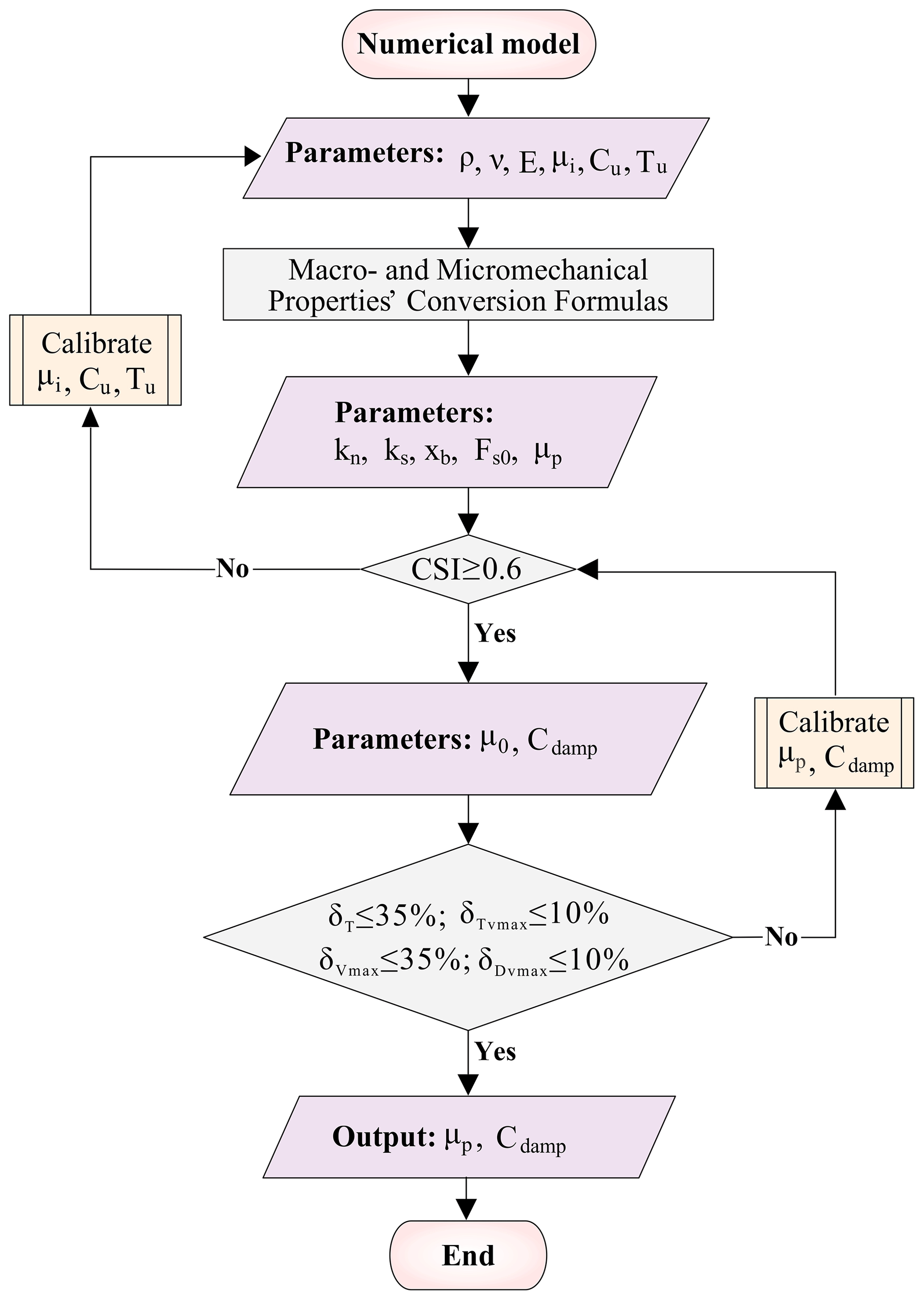
Figure 5Flowchart of the method of discrete-element parameter adjustment based on seismic signal inversion.
The second step is to use the geometry of the deposits as a reference to adjust and obtain reasonable simulation result. For the discrete-element method, the geometry of the deposits is affected by the bond strength between particles and the friction coefficient (An et al., 2020), which correspond to the fracture displacement, initial shear force, and friction coefficient between particles in MatDEM. Other parameters, such as normal stiffness and tangential stiffness, remain constant during the simulation. Accuracy of the final landslide accumulation was evaluated by the critical success index (CSI) proposed by Mergili et al. (2017a), calculated as follows:
where TP (true positive) is intersection area from both simulation and filed observation, FN (false negative) is the deposition area observed from field that simulation cannot covered, and FP (false positive) is the additional deposition area from simulation where no deposition is observed from site. CSI ranges between 0 and 1 (the higher the value, the more accurate the simulation); when CSI is 1, the simulated accumulation range coincides with the observed. An et al. (2021) conducted 25 simulations by changing parameters such as static friction coefficient, thermal weakening friction coefficient, and normal bond strength. The results showed that only eight cases had CSI > 0.6 and the highest CSI was 0.83. In addition, among the 15 groups of results simulated by Mergili et al. (2017b), the maximum CSI is 0.59. Therefore, in this study, the criterion is chosen as CSI > 0.6, and the simulated accumulation characteristics can be considered to be basically consistent with the actual situation.
The third step is to use the landslide motion velocity and displacement characteristics inverted by the seismic signal as a reference to back-calibrate parameters that affect the kinematic characteristics of the landslide, such as friction and average damping coefficients. The final values of the parameters are shown in Table 1.
Table 1Macro- and micro-mechanical parameters of Baige landslide material used in the discrete-element model.
The accuracy of simulated and inversed landslide velocity and displacement was preliminarily evaluated by the relative errors of several key points δ. Then, the square residue S2 between the simulated value and the inversion value per second was calculated, and the difference between the two groups of data in the landslide process was analyzed in detail. Related error δ and square residue S2 were calculated as follows:
where Xs is the simulated value and Xi the inversed value. X can be replaced by landslide duration T, peak velocity Vmax, time when peak velocity achieved , and peak displacement Dmax.
4.1 Seismic signal analysis
The time domain velocity curve of the seismic signal generated by the 10.10. Baige landslide is shown in Fig. 6. The SNR of the vertical (V) and east (E) components is relatively high compared to the north (N) component, roughly reflecting the main slide directions of the landslide being E and N. The post-event geological survey showed sliding was mainly in the southeast-to-south direction, approximately eastwards. The driving force of the landslide is gravity, and the surface on which the mass slides is inclined at about 35∘, thus velocity changes in the longitudinal direction are relatively large, and the SNR of the V component of the landslide signal appears high. The morphology of the landslide path means that the landslide stage has a large east–west component and a small north–south component, and in the deposition stage this reverses. This feature is consistent with the high SNR of the N component at the end of the landslide signal and low SNR of the E component.
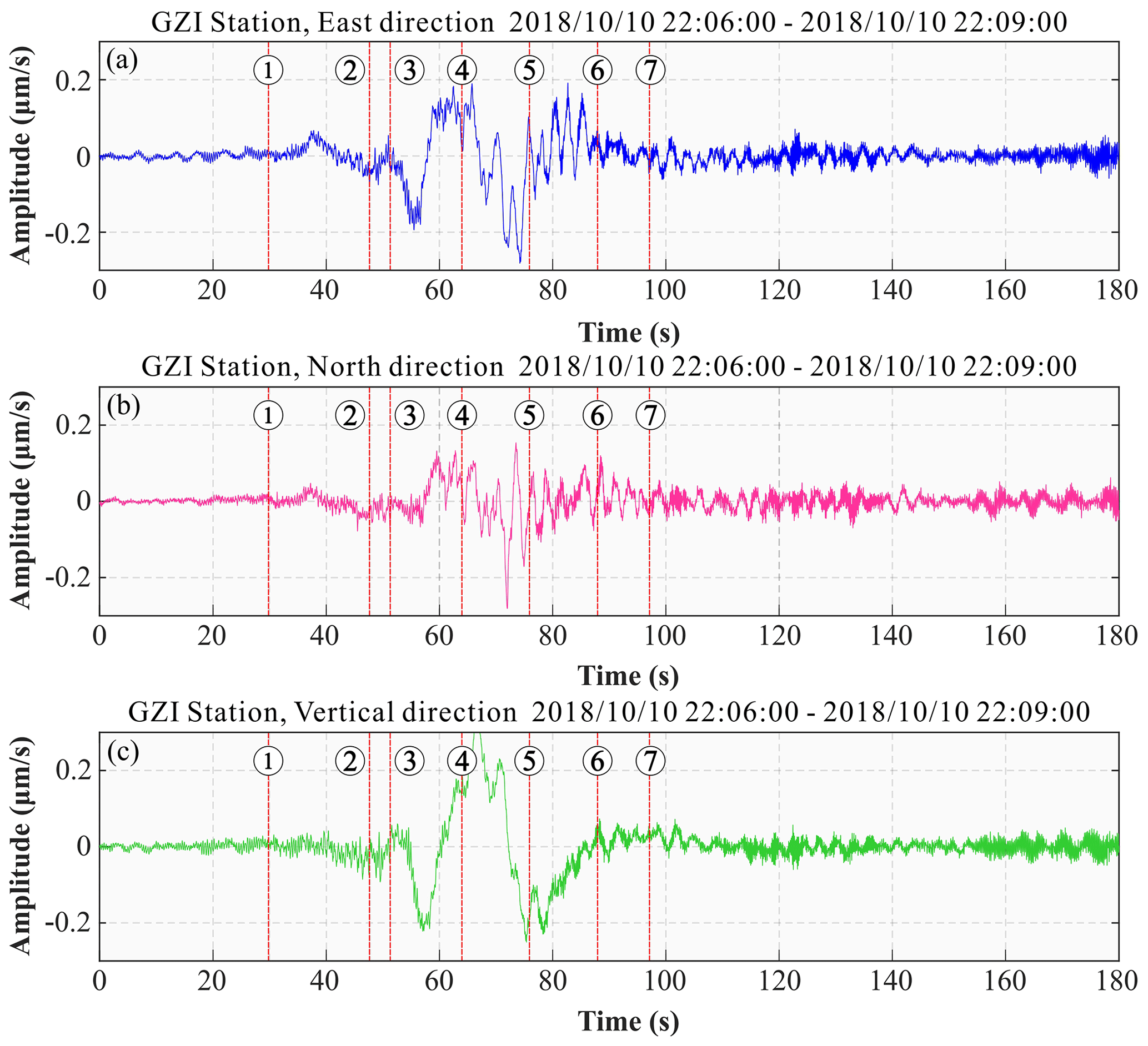
Figure 6Time domain velocity signal (E\N\V direction) of the seismic generated by the Baige landslide at GZI seismic station, visually showing a relatively high signal-to-noise ratio. The points labeled (1)–(7) refer to the characteristic stages of the Baige landslide.
Table 2The beginning characteristic stage of the Baige landslide river blocking event picked by seismic signal recorded at GZI station (all times are UTC+8).

The sliding distance of the landslide was ca. 600 m longitudinally and ca. 100 m laterally, while the receiving stations are over 100 km away; as the sliding scale is relatively small relative to the propagation distance, we treated it as a point source. The velocity curve recorded at a seismic station is the velocity of the crustal vibration below the landslide area propagating to the station, and this is roughly determined by velocity and mass of the landslide body. Therefore, characteristics of the landslide downward movement can be obtained by analyzing the velocity curve recorded at seismic stations. The seismic signal from station GZI (Fig. 6) provides an example to show the general seismic characteristics of the 10.10. Baige landslide. The time domain velocity curve recorded at GZI determines the start time of the landslide as 22:06 on 10 October 2018 (all times are UTC+8), with a duration of about 76 s between 22:06:39 and 22:07:51. Five points of velocity change are apparent during the landslide process (Fig. 6, Table 2), dividing the event into three phases of acceleration and three of deceleration.
Due to seismic wave propagation, the start time determined by the original seismic signal at the station is slightly later than the true time; what's more, the signal is mixed by longitudinal wave that stack with transverse wave, which makes the ending time picked by seismic signal much latter than the actual time. All these make the duration of the landslide derived from the original seismic signal would be lagged and longer, compared to the real time. A more accurate landslide duration can be determined by landslide force history inversion as it eliminates the propagation effect. The analysis of the velocity curve recorded at seismic stations helps us to understand the overall characteristics of the landslide and helps to verify the rationality of the subsequent Green's function stress inversion results.
The start and end time of sliding is demarcated on the time spectrum of the seismic curve (Fig. 7): strong energy clusters appear around 22:06:39, the intensity begins to decrease at 22:06:54 (UTC+8), and the frequency band narrows and the energy disappears at 22:07:27 (UTC+8). The time spectrum shows the landslide was concentrated between 22:06:40 and 22:07:01. The frequency is concentrated in the 0–1 Hz range, and the low-frequency component has a high SNR (0–0.2 Hz), which is conducive to dynamic inversion.
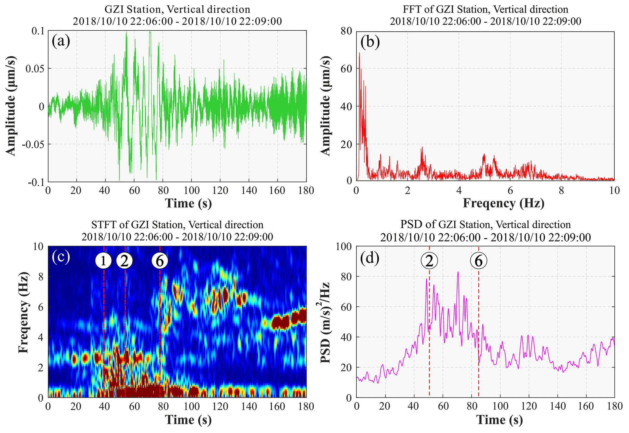
Figure 7Seismic signals of the Baige landslide as recorded at seismic station GZI. (a) Vertical seismic signal; (b) frequency spectrum; (c) time–frequency spectrum and the key times picked frequency from it, i.e., start time, first acceleration, and third deceleration, from left to right respectively; and (d) power spectral density (PSD) curve and the key times picked from it, i.e., first acceleration and third deceleration.
In Fig. 7d, the PSD curve is divided into three stages in the longitudinal direction, with the first and third stages corresponding to slow sliding and the second stage to fast sliding. Compared with the time domain stages (as in Table 2), the first PSD stage corresponds to the first acceleration and deceleration; the second stage corresponds to the second deceleration, acceleration, and third deceleration; and the third stage corresponds to the third deceleration. The PSD curve shows a marked increase in the second stage, indicating rapid downslope sliding, with multiple large fluctuations indicating rapid changes in landslide movement that are characteristic of the sliding stage.
According to Yan et al. (2021), the frequency of landslide hazard seismic signals is usually low (0–5 Hz), and the morphology in the time–frequency domain and time domain presents single-peak or double-peak characteristics, whereas the frequency of flood or high-density-flow seismic signals is usually high (5–50 Hz), and its morphology in the time–frequency domain and time domain is mostly flat. Combined with this, landslide seismic signal has relatively low frequency (0–1 Hz), and the single-peak feature in time and time-frequency characteristics is apparently different from the spectrum (main frequency: 15–30 Hz) of the outburst flood signal on 12 October 2018 (Xu et al., 2018). Therefore, we think that there was no flood discharge during the landslide process.
4.2 Dynamic inversion of landslide
Seismic data were processed using the following procedure before carrying out the landslide force history inversion. Firstly, they were deconvolved with the instrument response to obtain displacement. Following this, fourth-order Butterworth bandpass filter in the frequency band of 0.006–0.2 Hz was then applied. Finally, the records were resampled at a sampling rate of 5 Hz. The processed seismic records have a high SNR, as shown in Table 3. A total of 16 seismic traces with an SNR larger than 10 dB were selected to carry out the inversion.
Table 3SNR of seismic signals used in the inversion and CC and VR of the inversion results.
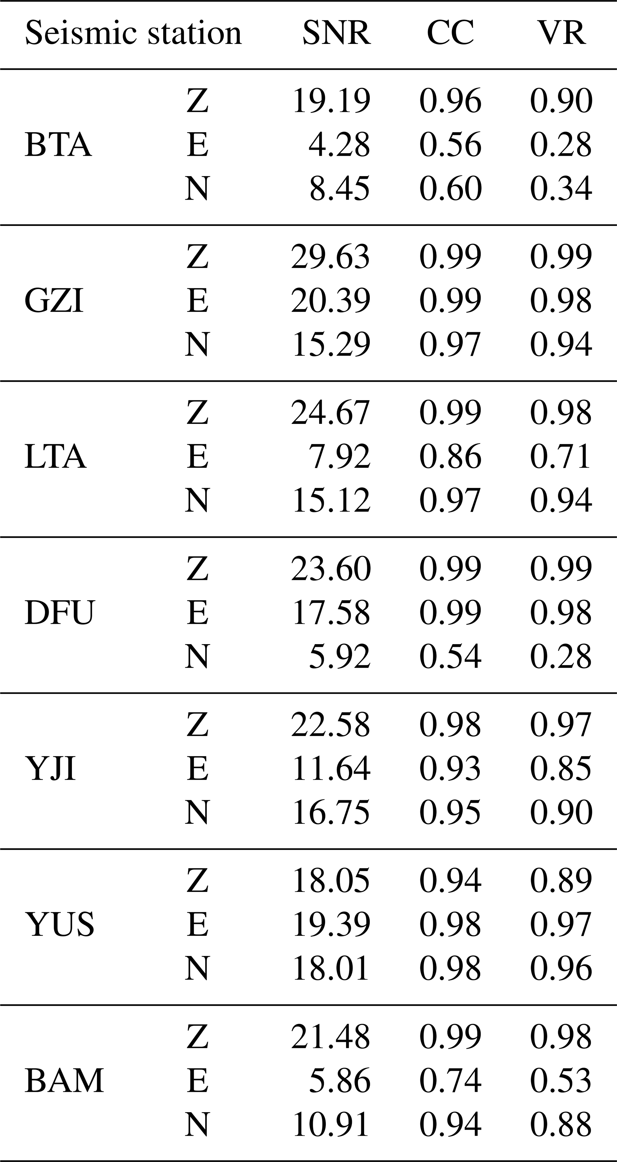
The inverted force histories are shown in Fig. 8. The good fit of the synthetic and recorded seismic waveforms in Fig. 9 and the high cross-correlation (CC) and variance reduction (VR) between synthetic and recorded seismograms provided in Table 3 indicate the high quality of the inversion results. The inverted forces show landslide initiation at , with a ∼61 s duration of the main motion.
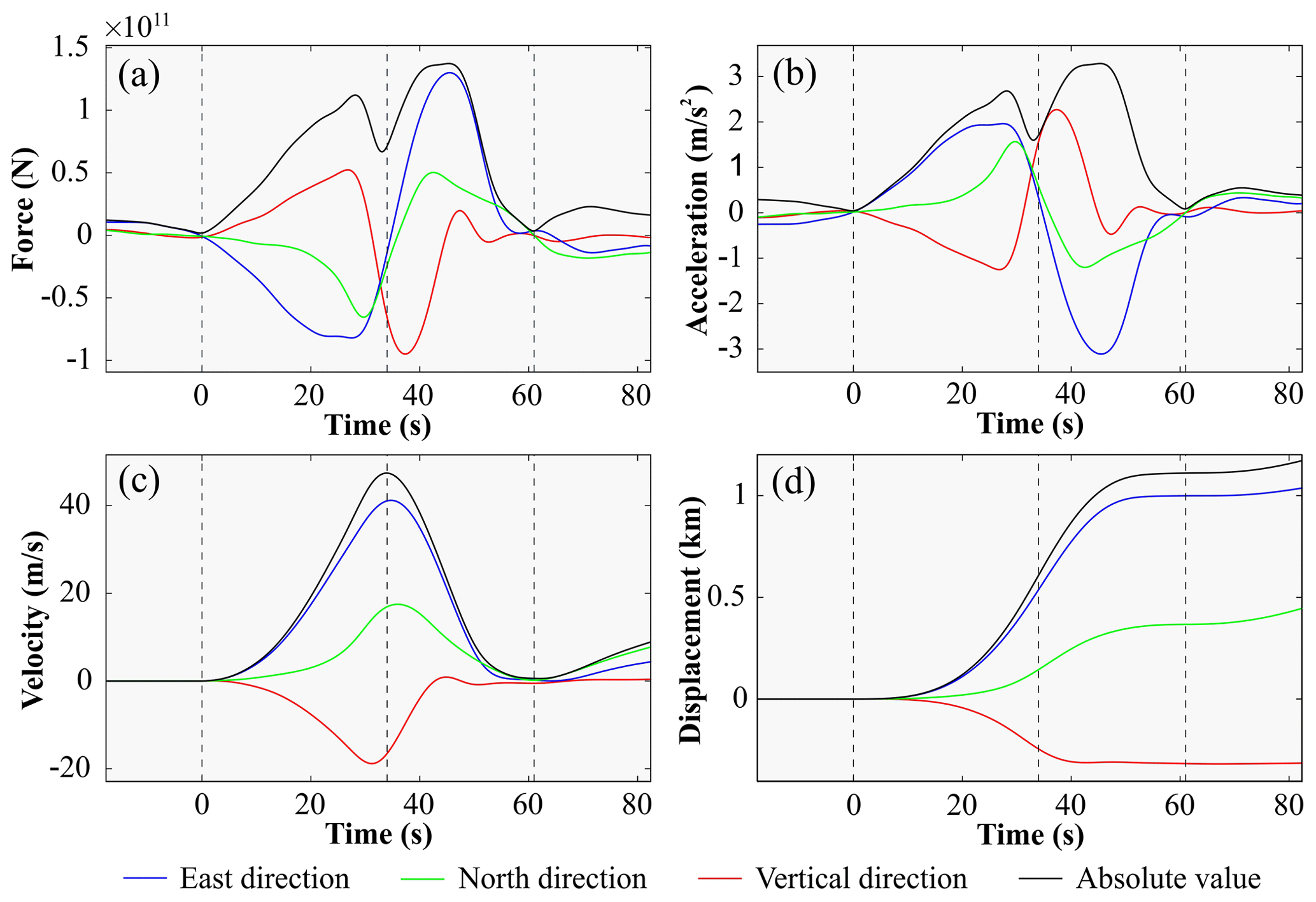
Figure 8Dynamic inversion used to obtain the Baige landslide characteristics: (a) inverted force–time history, (b) estimated acceleration distribution over time, (c) reconstructed velocity distribution over time from the inverted landslide force–time history, and (d) reconstructed displacement distribution over time from the inverted landslide force–time history. Corresponding absolute values are shown as black lines. Dashed vertical black lines mark the landslide start and end times (the left and right lines) and the time that the sliding mass reached the maximum speed (the middle line).

Figure 9Seismograms of the Baige landslide. Synthetic (red lines) and recorded (black lines) seismograms are compared. Dotted red lines indicate that the seismic trace was not used in the inversion because their SNR is smaller than 10 dB. Station name, distance from study site (km), and azimuth (degree) are given to the left of each trace (see Fig. 1d for locations), and the maximum amplitude of the three components is given (in µm) to the right.
By comparing the DEMs before and after the event, we determined the mass centers of the source area and the depositional area and subsequently derived the displacement of the center of the sliding mass. Following this, by minimizing the predicted and actual displacements, we estimated the sliding mass as 4.2×10¹⁰ kg. The recovered sliding trajectory fit well with the observations shown in Fig. 10. We used the estimated sliding mass to determine the acceleration and velocity distributions over time (Fig. 8b–d).
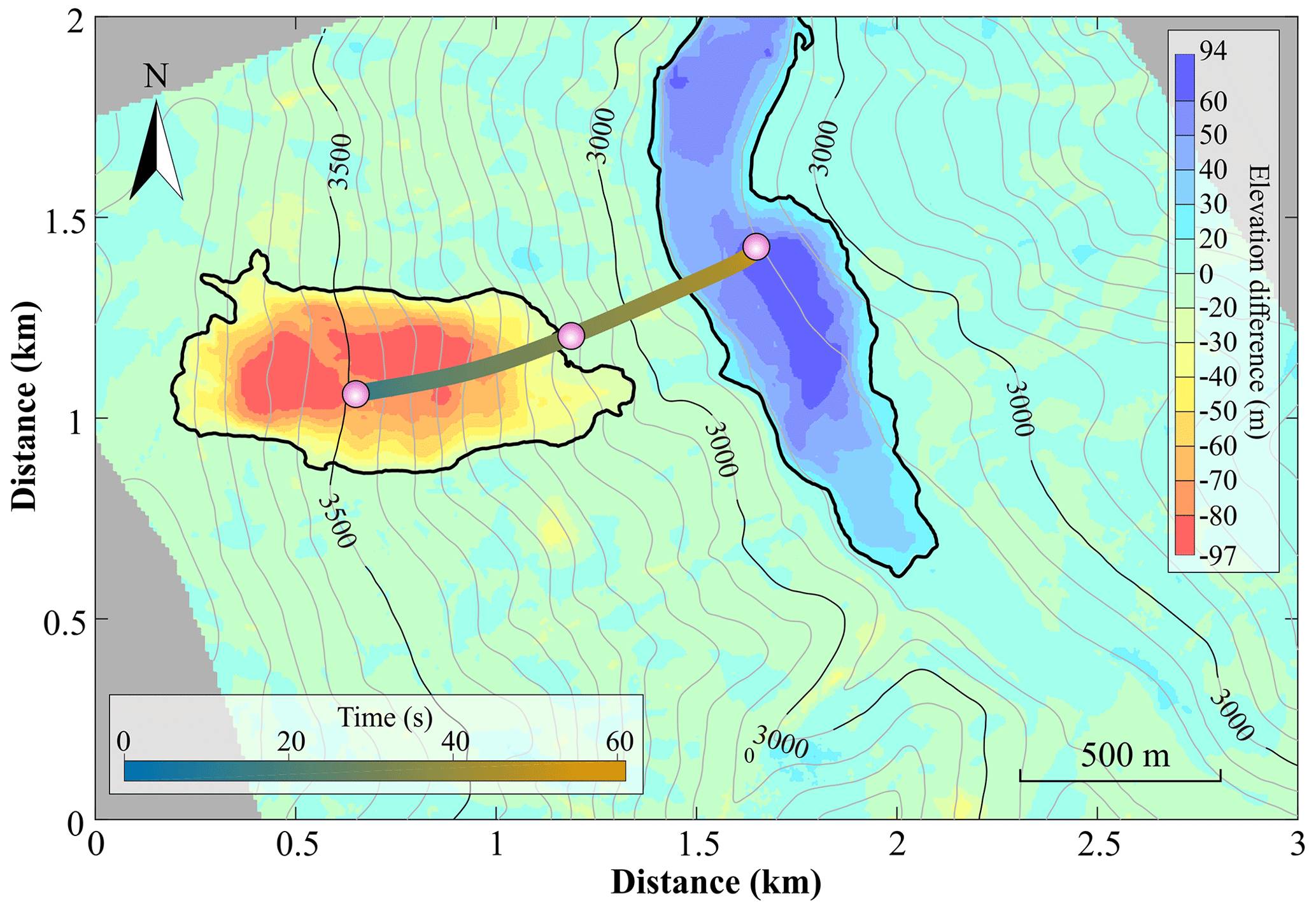
Figure 10Reconstructed horizontal trajectory of the Baige landslide from the seismic dynamic inversion. The base map is the elevation difference derived from DEMs, and the reconstructed trajectory is shown by the colored dots and connecting timeline.
The inversion results show two stages of landslide movement, 34 s of acceleration followed by 27 s of deceleration, which are separated by the vertical dashed black lines in Fig. 8. The sliding mass reached a maximum velocity of 47.4 m s−1 at the end of the acceleration stage and then rapidly decelerated (Fig. 8c). At ca. 50 s, the vertical component shows reverse force and velocity, indicating this was when the main sliding mass traveled over the Jinsha River. The force of the E and V components increases in a nearly linear manner in the first 26 s but then decreases rapidly. The reconstructed horizontal trajectory of the landslide (Fig. 10) indicates that the front of the sliding mass ran up the opposite valley wall after it crossed the Jinsha River.
4.3 Numerical modeling results
According to the results of numerical simulation, the movement process of the 10.10. Baige landslide can be divided into three stages: (1) sliding (0–20 s), (2) acceleration when entering the river (20–40 s), and (3) diffusion and accumulation (40–80 s). The velocity distribution through each stage of the simulated landslide is shown in Fig. 11.
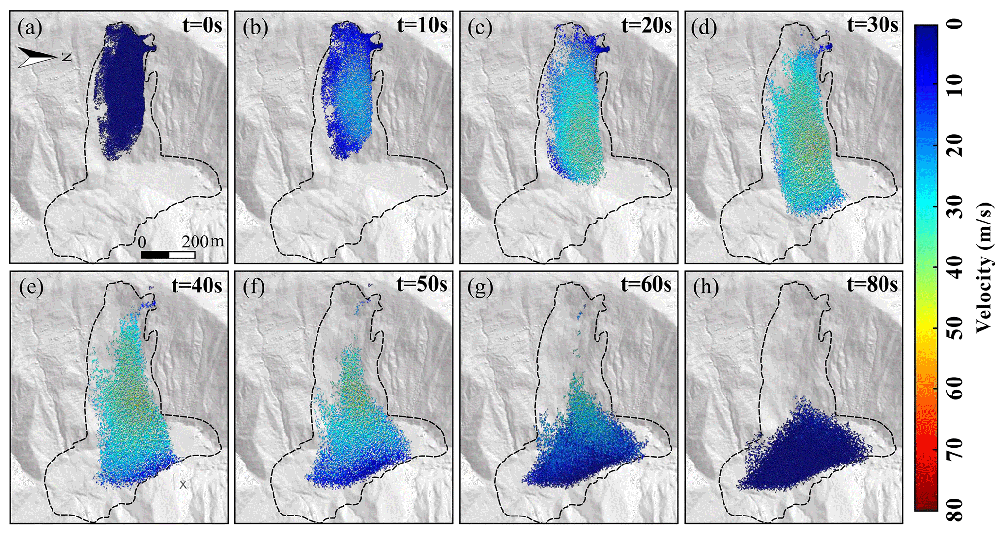
Figure 11Simulated landslide velocity distribution calculated in MatDEM: (a) t=0 s, (b) t=10 s, (c) t=20 s, (d) t=30 s, (e) t=40 s, (f) t=50 s, (g) t=60 s, (h) t=80 s. The digital terrain model (DTM) data of Fig. 11 are from the authors' own UAV photography measurements.
At the start of the simulation, the connection between particles inside and outside the sliding source area was broken simultaneously to initiate the landslide, which then rapidly fell with a constant (gravitational) acceleration. Due to the small particle friction coefficient (0.0897), simulated average velocity and average displacement growth rate are both higher than that determined in the inversion until 18 s, but their variation trends are similar. From the square residue results, there is little difference between the simulated and inverted landslide velocity and displacement at this stage, as shown in Fig. 12.
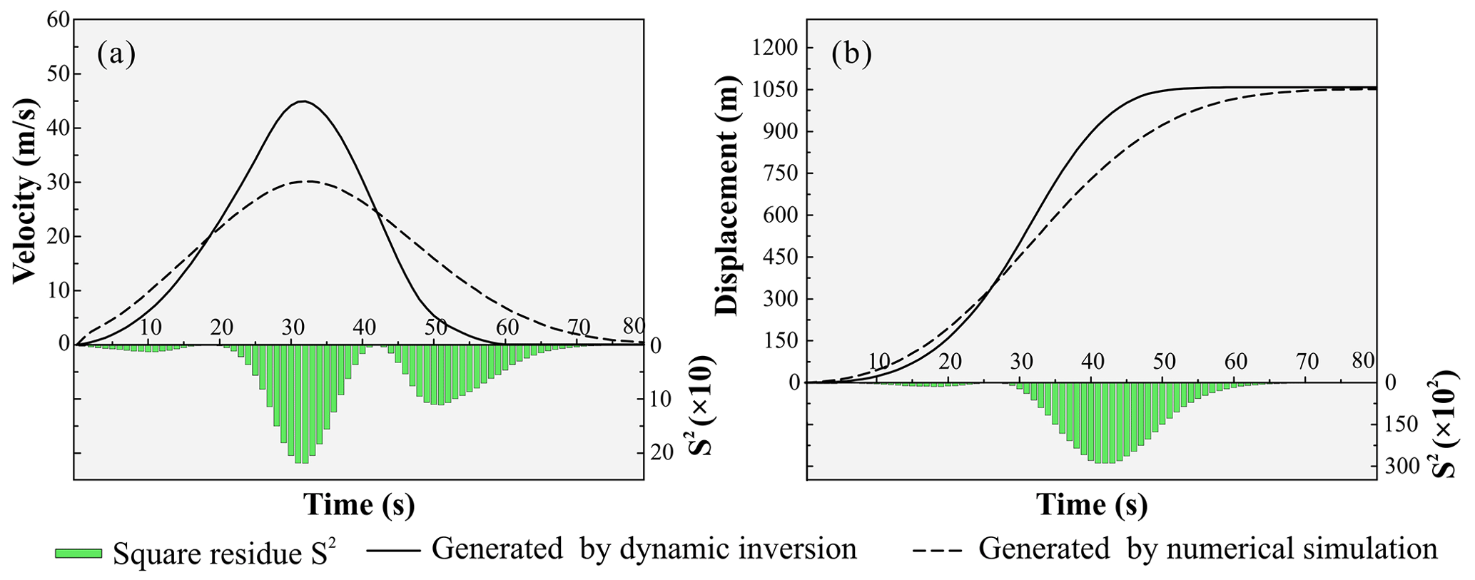
Figure 12Comparison of landslide characteristics simulated using discrete-element model with inversion results: (a) average velocity and (b) average displacement.
In the second stage, the landslide body is moving downwards at a constant acceleration in the simulation, but the inversion shows increased acceleration. Therefore, simulated average velocity and displacement appear to be substantially lower than the inversion. However, the time to reach peak velocity is similar for the simulation (32.8 s) and inversion (32 s). For both velocity and displacement, square residue between the inversion and simulation reaches a maximum in this stage, with S2 of 2.19×10² and 2.88×10⁴. At 40 s, the particles at the front edge of the landslide are stationary due to the obstacle provided by the valley wall or mountain slope on the opposite bank of Jinsha River.
In the third stage, from 40 s, particles in the middle and rear of the landslide body continue to move downwards, spreading and accumulating along the river, with a constant deceleration. After 60 s, the simulated average displacement reaches 1020 m and levels off thereafter, which corresponds well with the inversion. Most particles in the landslide body have accumulated and are stationary at this stage, but a few particles on the trailing edge are still moving. By 80 s, the average velocity tends to 0, showing that landslide movement has ended. The square residue of velocity residuals has a secondary peak around 50 s, while the displacement square residue decreases gradually. Overall, the simulated accumulation area is relatively small compared with that derived from DEM differencing, although the location of maximum thickness corresponds well (Fig. 13b). The CSI is calculated as 0.65, which suggests the simulation is moderately good.

Figure 13Comparison of elevation change associated with the Baige landslide (a) estimated from pre- and post-failure topography and (b) calculated using the discrete-element model. The remote sensing image map data of (a) and (b) are from the © Google Earth 2017.
5.1 Field observation and dynamic inversion
Using the empirical relationships of Chao et al. (2016) and Ekström and Stark (2013), the maximum inverted force of 1.37×10¹¹ N gives an estimated sliding mass of 5.5×10¹⁰ and 7.4×10¹⁰ kg, respectively, which are about 1.32 and 1.77 times our estimation of about 4.2×10¹⁰ kg from landslide force inversion. We further use a density of 2.4×10³ kg m−3 (Zhang et al., 2019) to estimate the volumes corresponding to these masses. The results are 1.75×10⁷, 2.29×10⁷, and 3.08×10⁷ m3, accounting for 89 %, 117 %, and 157 % of that derived from DEM differences, respectively. All estimated volumes are consistent with the DEM-derived volume in general, only that the estimates from empirical relationships are slightly larger. This is not surprising as we used a different frequency band in our inversion (0.006–0.2 Hz) than the two studies, e.g., Ekström and Stark (2013) used the frequency band 0.0067–0.0286 Hz (35–150 s). Previous work has shown that, for a given event, use of different frequency bands produces landslide force histories of different amplitudes (Hibert et al., 2014; Moore et al., 2017; Z. Zhang et al., 2020). As a comparison, we performed inversion in the frequency band 0.0067–0.0286 Hz, which gave a maximum force of 1.03×10¹¹ N and sliding mass estimates of 4.20×10¹⁰ and 5.60×10¹⁰ kg that are more consistent with our estimation. The newly estimated volumes from empirical relationships are also closer to the DEM-derived volume, accounting for 89 % and 119 %, respectively. Since the frequency bands that we used in the two inversions have similar lower cutoff frequencies, both of which include the duration of sliding (Gualtieri and Ekström, 2018; Toney and Allstadt, 2021), the kinematic parameters estimated from both inversion results are essentially similar in their characterization of overall landslide motion. We used the frequency band including relatively high-frequency energy (up to 0.2 Hz) in the inversion to allow for finer-scale characteristics of the forces and landslide motion to be analyzed (Zhao et al., 2015), such as the near-linear increase of the vertical component force in the first 26 s and subsequent abrupt decrease.
5.2 Link with numerical modeling
The numerical simulation combining signal inversion and field data more realistically reflects the landslide process than that based on field data alone. Differencing of pre- and post-landslide terrain data is commonly used to calibrate discrete-element simulations; however, it is a recognized limitation that this method does not inform on whether the landslide process is correctly modeled. Different combinations of discrete-element parameters may produce very similar superposition results even if the motion processes differ. In this study, the simulation is calibrated by the accumulation characteristics, and then the landslide movement process is further constrained by the inversion of the seismic signal. The final simulation results produced CSI of 0.65, of 2.5 %, δDmax of 0.6 %, δT of 33.3 %, and δVmax of 33.3 % (: error in time corresponds to peak velocity from simulated and inversed; δDmax: error in peak displacement from simulated and inversed; δT: error in time of landslide from simulated and inversed; δVmax: error in peak velocity from simulated and inversed), indicating they reflect the whole process of movement and accumulation well, overcoming the limitations of traditional methods.
Differences in the kinetic characteristics of different landslide phases between the numerical simulation and inversion are highlighted using analysis of square residue (Fig. 12). For example, the inversion results simulate the sliding stage (0–20 s) best, the diffusion and deposition stage (40–80 s) second best, and the acceleration stage (20–40 s) least. The good simulation of the sliding stage may be due to the fracture zone not yet being completely detached, so landslide movement is dominated by sliding of the whole body, which the theoretical assumption in the inversion approach. In the acceleration stage of large-scale landslides, friction between the sliding rock and soil and the base generates heat, which causes thermal compression and fluidization, leading to soil weakening (Wang et al., 2017, 2018). Reduction in the friction coefficient means the landslide moves faster; however, this factor is not considered in the current inversion model, so it underestimates peak velocity (Fig. 12). Despite the differences in kinematics, the simulation is essentially consistent with reality in terms of accumulation and movement characteristics.
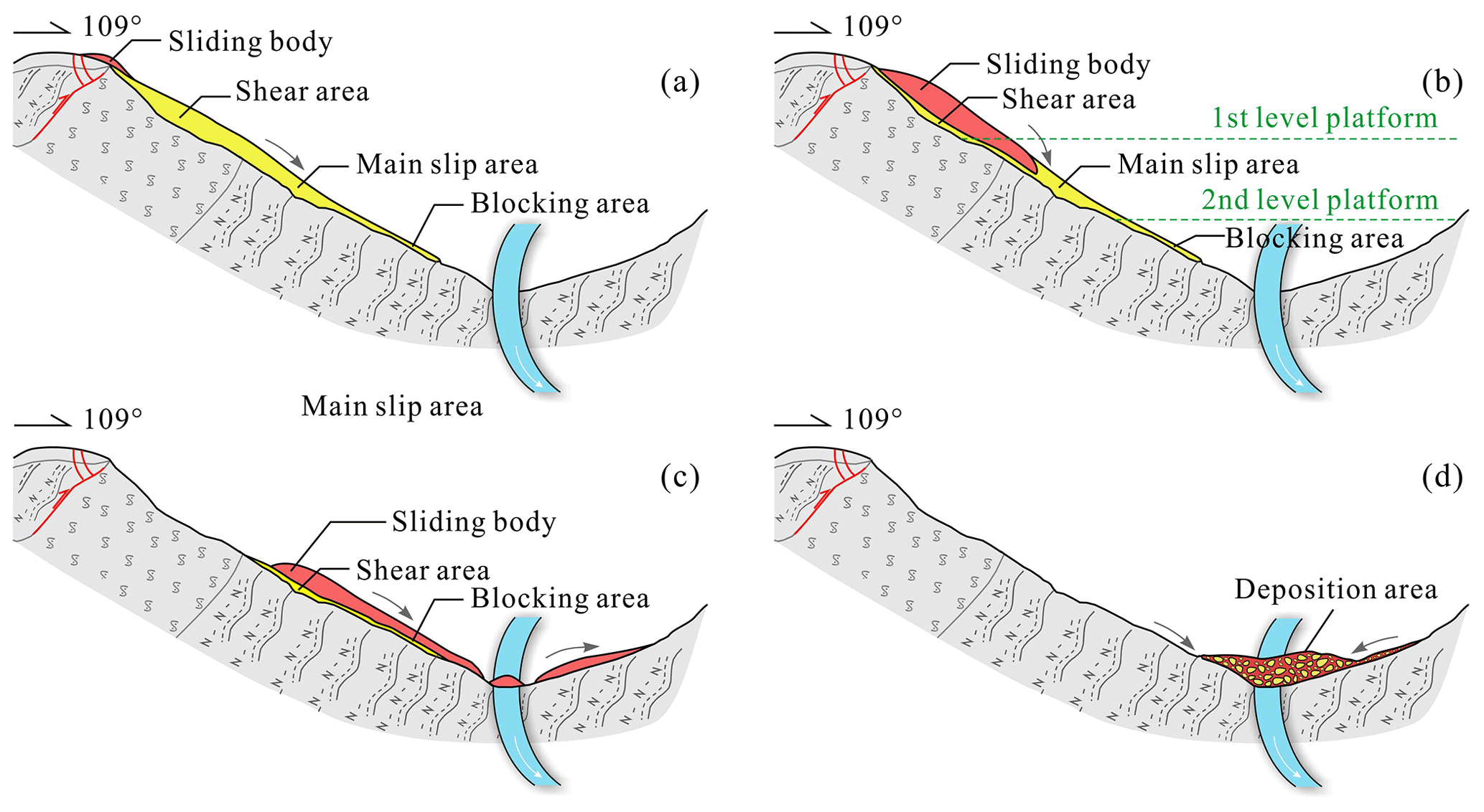
Figure 14Schematic diagram of the Baige landslide model: (a) stage 1 – initiation; (b) stage 2 – main slip; (c) stage 3 – crawling up against the slope (blocking); and (d) stage 4 – falling back and accumulation (deposition).
5.3 Reconstruction of landslide process
The Baige landslide has been the focus of much previous research (Xu et al., 2018; Deng et al., 2019; Fan et al., 2019a; Ouyang et al., 2019; Zhang et al., 2019; W. Wang et al., 2020); however, this study is the first analysis that couples seismic signal analysis, dynamic inversion, and numerical simulation. Our approach of multi-method mutual verification effectively reduces the inherent ambiguity of each method, and multi-method analysis improves the rationality and reliability of the results. Based on the characteristics of the 10.10. Baige landslide derived from our seismic signal inversion and discrete-element model simulation analysis, we have developed a generic model of landslide dynamics (Fig. 14). Our findings show the landslide was triggered by detachment of the weathered layer with severe top fault segmentation and that the landslide process comprised four stages: initiation, main slip, blocking, and deposition, as outlined below.
-
Initiation stage (Fig. 14a). The fracture zone on the upper part of the first-level platform loses stability and slides down under the action of gravity. Landslide debris is hindered by friction on the surface of the main sliding zone, so the landslide body moves relatively slowly. Increasing debris accumulates on the first-level platform and the lower main sliding area, which increases instability of the weathered layer, and other debris continues to fall downslope. The surface weathering layer of the main sliding area starts to slide, and the landslide body forms after the first fracture in the fracture development zone. Cascading from the initial fracture, continuous fracturing and sliding of the shear zone causes the landslide body to gradually increase; sliding of the top surface of the main sliding zone increases the scale of the landslide body. Downward sliding gradually accelerates as the landslide body increases, but friction in the main sliding area then acts to decelerate the mass; the deceleration process can be seen in the signal recorded at seismic station GZI (Fig. 7). As a result, acceleration increases slowly over ca. 10 s. This is evident in both the inversion and numerical simulation results.
-
Main slip stage (Fig. 14b). The main sliding area gradually loses stability and slides rapidly under the control of structural surfaces formed by weathering. The landslide body passes through the main sliding area and enters the wide and gentle second-level platform where resistance is relatively high. After crossing the second-level platform, the landslide enters the slip resistance zone where the degree of weathering is relatively weak, so the scouring action of the landslide body drives resistance. The effect of both sliding and anti-slip zones on the landslide body is relatively weak and is characterized well by the seismic signal in the time domain and the inverted acceleration curve. The initial sliding stage of the main sliding zone is reflected in the gradually increasing acceleration that peaks when the landslide body reaches the second-level platform and then decreases. When acceleration is approximately zero, the front part of the landslide has entered the river and the velocity of the landslide body peaks. The timing of maximum velocity in the inversion and simulation is consistent at 32 and 34 s, respectively (Fig. 12a).
-
Blocking stage (crawling up the opposite valley wall) (Fig. 14c). After passing through the anti-slip area, the landslide detaches at high speed at an altitude of ca. 2950 m and loses the support of the ground surface. Part of the landslide body accumulates in the river, and part hits the opposite (left) bank of the Jinsha River at a high speed and crawls upwards against the valley slope. During the upward movement, landslide debris spreads upstream and downstream, scouring the left bank of the river (SA3 in Fig. 1c) and a small area of the right bank (SA4 in Fig. 1c). Landslide debris reaches a maximum elevation of 3045 m on the opposite slope, then slides downslope under the action of gravity, forming debris strips like the scratches found on the sliding surface. Some debris remains on the relatively gentle slope of the left bank. The main feature of this process is that the action of gravity changes the force of the landslide body from dynamic to resistance; this is well reflected in the time domain seismic curve and inversion results (Fig. 8), where the acceleration switches rapidly from increasing to decreasing over ca. 10 s. As the upward crawling situation was not considered in the model design, the numerical simulation failed to describe the process.
-
Deposition stage (Falling back and accumulation) (Fig. 14d). Debris rapidly falls back down under the action of gravity, colliding with debris in the traction area of the river channel and interacting with stream flow to form a jet stream. Some finer particles in the landslide body mix with the sandblasting water to form a water–sand jet that discharges diagonally across the river toward the downstream left bank (SA5 in Fig. 1c) and upstream right bank (SA4 in Fig. 1c). Most of the detrital material stops moving and is deposited in the river channel, forming a barrier dam that starts to pond water. Under gravity and the action of water flow, small fragments at the top of the dam body lose stability and form a secondary slip zone (SA1 and SA2 in Fig. 1c) that becomes a drainage channel. The acceleration change during this downturn is roughly the same as the change trend of the main sliding phase. Acceleration first gradually increases and then decreases to zero before entering the deceleration phase. The seismic curve in the time domain and the inverted acceleration curve both characterize this process well, and the inversion results give a duration of ca. 10 s.
5.4 Research contribution
A post-event geological survey can examine depositional characteristics of the landslide and weathering and fracture conditions of rocks in the slide source area, which provide some information for understanding landslide causal processes. The seismic signal provides some information on landslide evolution. The low-frequency component reflects the overall movement trend of the landslide, and the high-frequency component reflects detailed characteristics of the movement process. Experienced researchers can reconstruct the landslide process using a combination of geological survey and seismic signal analysis. However, the propagation effect of the stratum means that the seismic signal does not completely correspond to landslide movement, may generate false images, and confounds precise determination of landslide start time and duration.
Landslide dynamic inversion based on the long-wavelength information of the seismic signal eliminates the propagation effect, which allows the dynamic parameter curve of the landslide to be obtained, giving a relatively accurate determination of landslide start and end time and event duration. The dynamic inversion result reflects the change process of the overall movement trend of the landslide (the low-frequency trend) and can be used to verify the results of combined geological survey and seismic signal analysis. The low-frequency (0–0.2 Hz) component of dynamic parameters, as provided by dynamic inversion, can guide the all band frequency motion, constraining the high-frequency (>0.2 Hz) movement analysis of the landslide process, which helps to reduce ambiguity.
The accuracy of numerical simulation results depends on scientific models and accurate parameters. When static parameters such as pre- and post-landslide topography are used to select parameters and constrain results of numerical simulation, there are often multiple solutions. The accuracy of the landslide dynamic with time evolution process will not be determined using only the calibration of the depositional morphology because different velocities and evolutionary processes may produce similar accretionary landforms (An et al., 2021; Mergili et al., 2017b), especially for large-scale landslides like Baige, which occur next to deeply incised valleys. Compared with the study of An et al. (2021), which mainly focuses on force–time history inversion, we further added the velocity and displacement characteristics retrieved from seismic signals to conduct dynamic quantitative constraints on dynamic parameters and improve the credibility of numerical simulation to carry out efficient simulation of landslide process. The improved simulation allows for in-depth analysis of frequency motion characteristics of the landslide, such as speed change, characteristics of each stage, etc. These characteristics can also be used to verify and optimize the landslide process to improve analysis results.
Each of the three methods has disadvantages which may lead to errors and ambiguities in analyzing landslides. However, the combined use and mutual verification of the different methods can effectively avoid ambiguity and improve the reasonableness of results.
In this study, we used an on-site geological survey, landslide seismic signal analysis, dynamic inversion, and numerical simulation to provide a comprehensive analysis of 10.10. Baige landslide. We used a STFT and PSD to analyze the seismic signals for Baige landslide. We then reconstructed the landslide force history by direct deconvolution of the observed seismograms with Green's functions. We then developed a method that use seismic inversion to constrain and calibrate the numerical input parameters using discrete-element method. After calibrating the parameters of the numerical models, the dynamic process of the 10.10. Baige landslide was analyzed. Nevertheless, several key issues that are not considered in the discrete-element method (leading to differences between the simulation and inversion), such as friction coefficient decreases as the landslide progresses, base entrainment, and particle breakage, should be considered in future research.
There is an analytical solution between the macro- and micro-mechanical parameters of the tightly packed discrete-element model, i.e., the conversion formula proposed by Liu et al. (2013). For the linear elastic model, there are five micro-mechanical parameters, i.e., the normal stiffness (Kn), shear stiffness (Ks), breaking displacement (Xb), shear resistance (), coefficient of friction (μp) defined by Young's modulus (E), Poisson's ratio (v), tensile strength (Tu), compressive strength (Cu), and coefficient of intrinsic friction (μi). The conversion formulae are as follows:
All raw data can be provided by the corresponding authors upon request.
The supplement related to this article is available online at: https://doi.org/10.5194/esurf-10-1233-2022-supplement.
YY is the first author, responsible for most of the work and manuscript writing. YC is the second author and the corresponding author, responsible for the numerical simulation, processing and verification of the data, and manuscript writing. XH is the third author and is responsible for all dynamic inversion methods and technology implementation. JZ is the fourth author and is responsible for the production of the article figures and tables. WZ is the fifth author, responsible for checking the overall logical structure of the article. SY and JG are the sixth and seventh author, respectively, responsible for the numerical simulations. SH is the last author, responsible for reviewing and editing the manuscript.
The contact author has declared that none of the authors has any competing interests.
Publisher's note: Copernicus Publications remains neutral with regard to jurisdictional claims in published maps and institutional affiliations.
This study was financially supported by the National Natural Science Foundation of China (grant nos. 42120104002, 41901008, U21A2008, 41941019), the Second Tibetan Plateau Scientific Expedition and Research Program (STEP) (grant no. 2019QZKK0906), the Fundamental Research Funds for the Project of Science & Technology Department of Sichuan Province (grant no. 2020YFH0085), and the State Key Laboratory of Hydroscience and Hydraulic Engineering (No. 2021-KY-04).
The probabilistic power spectral densities are calculated and plotted using ObsPy (https://docs.obspy.org/, last access: 23 October 2021).
This research has been supported by the National Natural Science Foundation of China (grant nos. 42120104002, 41901008, U21A2008 and 41941019), the Second Tibetan Plateau Scientific Expedition and Research Program (STEP) (grant no. 2019QZKK0906), the Fundamental Research Funds for the Project of Science & Technology Department of Sichuan Province (grant no. 2020YFH0085), and the State Key Laboratory of Hydroscience and Hydraulic Engineering (grant no. 2021-KY-04).
This paper was edited by Xuanmei Fan and reviewed by Zheng-yi Feng and Marc Peruzzetto.
Allstadt, K.: Extracting source characteristics and dynamics of the August 2010 Mount Meager landslide from broadband seismograms, J. Geophys. Res.-Earth, 118, 1472–1490, https://doi.org/10.1002/jgrf.20110, 2013.
An, H. C., Ouyang, C. J., Zhao, C., and Zhao, W.: Landslide dynamic process and parameter sensitivity analysis by discrete element method: the case of Turnoff Creek rock avalanche, J. Mt. Sci., 17, 1581–1595, https://doi.org/110.1007/s11629-020-5993-7, 2020.
An, H. C., Ouyang, C. J., and Zhou, S.: Dynamic process analysis of the Baige landslide by the combination of DEM and long-period seismic waves, Landslides, 18, 1625–1639, https://doi.org/10.1007/s10346-020-01595-0, 2021.
Brodsky, E. E., Gordeev, E., and Kanamori, H.: Landslide basal friction as measured by seismic waves, Geophys. Res. Lett., 30, 2236, https://doi.org/10.1029/2003GL018485, 2003.
Chao, W. A., Zhao, L., Chen, S. C., Wu, Y. M., Chen, C. H., and Huang, H. H.: Seismology-based early identification of dam-formation landquake events, Sci. Rep., 6, 19259, https://doi.org/10.1038/srep19259, 2016.
Chen, C. H., Chao, W. A., Wu, Y. M., Zhao, L., Chen, Y. G., Ho, W. Y., Lin, T. L., Kuo, K. H., and Chang, J. M.: A seismological study of landquakes using a real-time broad-band seismic network, Geophys. J. Int., 194, 885–898, https://doi.org/10.1093/gji/ggt121, 2013.
Cui, Y., Fang, F., Li, Y., and Liu, H.: Assessing effectiveness of a dual-barrier system for mitigating granular flow hazards through DEM-DNN framework, Eng. Geol., 306, 106742, https://doi.org/10.1016/j.enggeo.2022.106742, 2022.
Dahlen, F. A.: Single-force representation of shallow landslide sources, B. Seismol. Soc. Am., 83, 130–143, https://doi.org/10.1785/BSSA0830010130, 1993.
Dammeier, F., Moore, J. R., Hammer, C., Haslinger, F., and Loew, S.: Automatic detection of alpine rockslides in continuous seismic data using hidden Markov models, J. Geophys. Res.-Earth, 121, 351–371, https://doi.org/10.1002/2015jf003647, 2016.
Darlington, W. J., Ranjith, P. G., and Choi, S. K.: The Effect of Specimen Size on Strength and Other Properties in Laboratory Testing of Rock and Rock-Like Cementitious Brittle Materials, Rock Mech. Rock Eng., 44, 513–529, https://doi.org/10.1007/s00603-011-0161-6, 2011.
Deng, J. J., Gao, Y. J., Yu, Z. Q., and Xie, H. P.: Analysis on the Formation Mechanism and Process of Baige Landslides Damming the Upper Reach of Jinsha River,China, Adv. Eng. Sci., 51, 9–16, https://doi.org/10.15961/j.jsuese.201801438, 2019.
Ekström, G. and Stark, C. P.: Simple scaling of catastrophic landslide dynamics, Science, 339, 1416–1419, https://doi.org/10.1126/science.1232887, 2013.
Fan, X., Yang, F., Subramanian, S. S., Xu, Q., Feng, Z., Mavrouli, O., Peng, M., Ouyang, C., Jansen, D., and Huang, R.: Prediction of a multi-hazard chain by an integrated numerical simulation approach: the Baige landslide, Jinsha River, China, Landslides, 17, 147–164, https://doi.org/10.1007/s10346-019-01313-5, 2019a.
Fan, X., Xu, Q., Liu, J., Subramanian, S. S., He, C., Zhu, X., and Zhou, L.: Successful early warning and emergency response of a disastrous rockslide in Guizhou province, China, Landslides, 16, 2445–2457, https://doi.org/10.1007/s10346-019-01269-6, 2019b.
Fang, J., Cui, Y., Li, X., and Nie, J.: A new insight into the dynamic impact https://doi.org/10.1016/j.compgeo.2022.104790, 2022.
Favreau, P., Mangeney, A., Lucas, A., Crosta, G., and Bouchut, F.: Numerical modeling of landquakes, Geophys. Res. Lett., 37, L15305, https://doi.org/10.1029/2010gl043512, 2010.
Feng, Z.: The seismic signatures of the 2009 Shiaolin landslide in Taiwan, Nat. Hazards Earth Syst. Sci., 11, 1559–1569, https://doi.org/10.5194/nhess-11-1559-2011, 2011.
Feng, Z. Y., Lo, C. M., and Lin, Q. F.: The characteristics of the seismic signals induced by landslides using a coupling of discrete element and finite difference methods, Landslides, 14, 661–674, https://doi.org/10.1007/s10346-016-0714-6, 2016.
Froude, M. J. and Petley, D. N.: Global fatal landslide occurrence from 2004 to 2016, Nat. Hazards Earth Syst. Sci., 18, 2161–2181, https://doi.org/10.5194/nhess-18-2161-2018, 2018.
Fuchs, F., Lenhardt, W., and Bokelmann, G.: Seismic detection of rockslides at regional scale: examples from the Eastern Alps and feasibility of kurtosis-based event location, Earth Surf. Dynam., 6, 955–970, https://doi.org/10.5194/esurf-6-955-2018, 2018.
Fukao, Y.: Single-force representation of earthquakes due to landslides or the collapse of caverns, Geophys. J. Int., 122, 243–248, https://doi.org/10.1111/j.1365-246X.1995.tb03551.x, 1995.
Gualtieri, L. and Ekström, G.: Broad-band seismic analysis and modeling of the 2015 Taan Fjord, Alaska landslide using Instaseis, Geophys. J. Int., 213, 1912–1923, https://doi.org/10.1093/gji/ggy086, 2018.
Hasegawa, H. S. and Kanamori, H.: Source mechanism of the magnitude 7.2 Grand Banks earthquake of November 1929: Double couple or submarine landslide?, Bull. Seismol. Soc. Am., 77, 1984–2004, 1987.
Helmstetter, A. and Garambois, S.: Seismic monitoring of Séchilienne rockslide (French Alps): Analysis of seismic signals and their correlation with rainfall, J. Geophys. Res., 115, F03016, https://doi.org/10.1029/2009jf001532, 2010.
Hibert, C., Ekström, G., and Stark, C. P.: Dynamics of the Bingham Canyon Mine landslides from seismic signal analysis, Geophys. Res. Lett., 41, 4535–4541, https://doi.org/10.1002/2014GL060592, 2014.
Hibert, C., Stark, C. P., and Ekström, G.: Dynamics of the Oso-Steelhead landslide from broadband seismic analysis, Nat. Hazards Earth Syst. Sci., 15, 1265–1273, https://doi.org/10.5194/nhess-15-1265-2015, 2015.
Jiang, Y., Wang, G., and Kamai, T.: Fast shear behavior of granular materials in ring-shear tests and implications for rapid landslides, Acta Geotech., 12, 645–655, https://doi.org/10.1007/s11440-016-0508-y, 2016.
Kanamori, H. and Given, J. W.: Analysis of long-period seismic waves excited by the May 18, 1980, eruption of Mount St. Helens – A terrestrial monopole?, J. Geophys. Res.-Solid, 87, 5422–5432, https://doi.org/10.1029/JB087iB07p05422, 1982.
Kanamori, H., Given, J. W., and Lay, T.: Analysis of seismic body waves excited by the Mount St. Helens eruption of May 18, 1980, J. Geophys. Res.-Solid, 89, 1856–1866, https://doi.org/10.1029/JB089iB03p01856, 1984.
Kao, H., Kan, C. W., Chen, R. Y., Chang, C. H., Rosenberger, A., Shin, T. C., Leu, P. L., Kuo, K. W., and Liang, W. T.: Locating, monitoring, and characterizing typhoon-induced landslides with real-time seismic signals, Landslides, 9, 557–563, https://doi.org/10.1007/s10346-012-0322-z, 2012.
Li, C. Y., Wang, X. C., He, C. Z., Wu, X., Kong, Z. Y., and Li, X. L.: China National Digital Geological Map (Public Version at 1:200 000 Scale) Spatial Database (V1), Development and Research Center of China Geological Survey; China Geological Survey (producer), 1957, National Geological Archives of China (distributor), https://doi.org/10.23650/data.A.2019.NGA120157.K1.1.1.V1, 2019.
Li, W., Chen, Y., Liu, F., Yang, H., Liu, J., and Fu, B.: Chain-style landslide hazardous process: Constraints from seismic signals analysis of the 2017 Xinmo landslide, SW China, J. Geophys. Res.-Solid, 124, 2025–2037, https://doi.org/10.1029/2018JB016433, 2019.
Li, Z., Huang, X., Xu, Q., Yu, D., Fan, J., and Qiao, X.: Dynamics of the Wulong landslide revealed by broadband seismic records, Earth Planets Space, 69, 27, https://doi.org/10.1186/s40623-017-0610-x, 2017.
Li, Z., Huang, X., Yu, D., Su, J., and Xu, Q.: Broadband-seismic analysis of a massive landslide in southwestern China: Dynamics and fragmentation implications, Geomorphology, 336, 31–39, https://doi.org/10.1016/j.geomorph.2019.03.024, 2019.
Liu, C., Pollard, D. D., and Shi, B.: Analytical solutions and numerical tests of elastic and failure behaviors of close-packed lattice for brittle rocks and crystals, J. Geophys. Res.-Solid, 118, 71–82, https://doi.org/10.1029/2012JB009615, 2013.
Liu, C., Xu, Q., Shi, B., Deng, S., and Zhu, H.: Mechanical properties and energy conversion of 3D close-packed lattice model for brittle rocks, Comput. Geosci., 103, 12–20, https://doi.org/10.1016/j.cageo.2017.03.003, 2017.
Liu, C., Fan, X., Zhu, C., and Shi, B.: Discrete element modeling and simulation of 3-Dimensional large-scale landslide-Taking Xinmocun landslide as an example, J. Eng. Geol., 27, 1362–1370, https://doi.org/10.13544/j.cnki.jeg.2018-234, 2019.
Liu, D. Z., Cui, Y. F., Wang, H., Jin, W., Wu, C. h., Nazir, AB., Zhang, G. T., Carling, P., and Chen, H. Y.: Assessment of local outburst flood risk from successive landslides: Case study of Baige landslide-dammed lake, upper Jinsha river, eastern Tibet, J. Hydrol., 599, 126294, https://doi.org/10.1016/j.jhydrol.2021.126294, 2021.
Lo, C. M., Lin, M. L., Tang, C. L., and Hu, J. C.: A kinematic model of the Hsiaolin landslide calibrated to the morphology of the landslide deposit, Eng. Geol., 123, 22–39, https://doi.org/10.1016/j.enggeo.2011.07.002, 2011.
McNamara, D. E. and Buland, R. P.: Ambient Noise Levels in the Continental United States, Bull. Seismol. Soc. Am., 94, 1517–1527, https://doi.org/10.1785/012003001, 2004.
Mergili, M., Fischer, J. T., Krenn, J., and Pudasaini, S. P.: r. avaflow v1, an advanced open-source computational framework for the propagation and interaction of two-phase mass flows, Geosci. Model Dev., 10, 553–569, https://doi.org/10.5194/gmd-10-553-2017, 2017a.
Mergili, M., Emmer, A., Juřicová A., Cochachin, A., Fischer, J. T., Huggel, C., and Pudasaini, S. P.: How well can we simulate complex hydro-geomorphic process chains? The 2012 multi-lake outburst flood in the Santa Cruz Valley (Cordillera Blanca, Perú), Earth Surf. Proc. Land., 43, 1373–1389, https://doi.org/10.1002/esp.4318, 2017b.
Moore, J. R., Pankow, K. L., Ford, S. R., Koper, K. D., Hale, J. M., Aaron, J., and Larsen, C. F.: Dynamics of the Bingham Canyon rock avalanches (Utah, USA) resolved from topographic, seismic, and infrasound data, J. Geophys. Res.-Earth, 122, 615–640, https://doi.org/10.1002/2016JF004036, 2017.
Moretti, L., Mangeney, A., Capdeville, Y., Stutzmann, E., Huggel, C., Schneider, D., and Bouchut, F.: Numerical modeling of the Mount Steller landslide flow history and of the generated long period seismic waves, Geophys. Res. Lett., 39, L16402, https://doi.org/10.1029/2012GL052511, 2012.
Moretti, L., Allstadt, K., Mangeney, A., Capdeville, Y., Stutzmann, E., and Bouchut, F.: Numerical modeling of the Mount Meager landslide constrained by its force history derived from seismic data, J. Geophys. Res.-Solid, 120, 2579–2599, https://doi.org/10.1002/2014JB011426, 2015.
Muceku, Y., Korini, O., and Kuriqi, A.: Geotechnical analysis of hill's slopes areas in heritage town of Berati, Albania, Period. Polytech. Civ. Eng., 60, 61–73, https://doi.org/10.3311/PPci.7752, 2016.
Ouyang, C. J., An, H. C., Zhou, S., Wang, Z. W., Su, P. C., and Wang, D. P.: Insights from the failure and dynamic characteristics of two sequential landslides at Baige village along the Jinsha River, China, Landslides, 16, 1397–1414, https://doi.org/10.1007/s10346-019-01177-9, 2019.
Pastor, M., Blanc, T., Haddad, B., Petrone, S., Sanchez, M. M., Drempetic, V., Issler, D., Crosta, G. B., Cascini, L., Sorbino, G., and Cuomo, S.: Application of a SPH depthintegrated model to landslide run-out analysis, Landslides, 11, 793812, https://doi.org/10.1007/s10346-014-0484-y, 2014.
Peterson, J. R.: Observations and modeling of seismic background noise, US Geological Survey Open-File Report 93-322, US Geological Survey, https://doi.org/10.3133/ofr93322, 1993.
Pitman, E. B., Nichita, C. C., Patra, A., Bauer, A., Sheridan, M., and Bursik, M.: Computing granular avalanches and landslides, Phys. Fluids, 15, 3638–3646, https://doi.org/10.1063/1.1614253, 2003.
Sakals, M. E., Geertsema, M., Schwab, J. W., and Foord, V. N.: The Todagin Creek landslide of October 3, 2006, Northwest British Columbia, Canada, Landslides, 9, 107–115, https://doi.org/10.1007/s10346-011-0273-9, 2011.
Shen, W., Li, T., Li, P., and Lei, Y.: Numerical assessment for the efficiencies of check dams in debris flow gullies: A case study, Comput. Geotech., 122, 103541, https://doi.org/10.1016/j.compgeo.2020.103541, 2020.
Sheng, M., Chu, R., Wang, Y., and Wang, Q.: Inversion of source mechanisms for single-force events using broadband waveforms, Seismol. Res. Lett., 91, 1820–1830, https://doi.org/10.1785/0220190349, 2020.
Soga, K., Alonso, E., Yerro, A., Kumar, K., and Bandara, S.: Trends in large-deformation analysis of landslide mass movements with particular emphasis on the material point method, Géotechnique, 66, 1–26, https://doi.org/10.1680/jgeot.15.lm.005, 2016.
Toney, L. and Allstadt, K. E.: lsforce: A Python-Based Single-Force Seismic Inversion Framework for Massive Landslides, Seismol. Res. Lett., 92, 2610–2626, https://doi.org/10.1785/0220210004, 2021.
Walter, M., Arnhardt, C., and Joswig, M.: Seismic monitoring of rockfalls, slide quakes, and fissure development at the Super-Sauze mudslide, French Alps, Eng. Geol., 128, 12–22, https://doi.org/10.1016/j.enggeo.2011.11.002, 2012.
Wang, L., Wu, C. Z., Gu, X., Liu, H. L., Mei, G. X., and Zhang, W. G.: Probabilistic stability analysis of earth dam slope under transient seepage using multivariate adaptive regression splines, Bull. Eng. Geol. Environ., 79, 2763–2775, https://doi.org/10.1007/s10064-020-01730-0, 2020.
Wang, R.: A simple orthonormalization method for stable and efficient computation of Green's functions, Bull. Seismol. Soc. Am., 89, 733–741, 1999.
Wang, W., Yin, Y., Zhu, S., Wang, L., Zhang, N., and Zhao, R.: Investigation and numerical modeling of the overloading-induced catastrophic rockslide avalanche in Baige, Tibet, China, Bull. Eng. Geol. Environ., 79, 1765–1779, https://doi.org/10.1007/s10064-019-01664-2, 2020.
Wang, Y. F., Dong, J. J., Cheng, Q. G.: Velocity-dependent frictional weakening of large rock avalanche basal facies: Implications for rock avalanche hypermobility?, J. Geophys. Res.-Solid, 122, 1648–1676, https://doi.org/10.1002/2016JB013624, 2017.
Wang, Y. F., Dong, J. J., Cheng, Q. G.: Normal stress-dependent frictional weakening of large rock avalanche basal facies: Implications for the rock avalanche volume effect, J. Geophys. Res.-Solid, 123, 3270–3282, https://doi.org/10.1002/2018JB015602, 2018.
Xu, Q., Zheng, G., Li, W. L., He, C. Y., Dong, X. J., Guo, C., and Feng, W. K.: Study on Successive Landslide Damming Events of Jinsha River in Baige Village on October 11 and November 3, 2018, J. Eng. Geo., 26, 1534–1551, https://doi.org/10.13544/j.cnki.jeg.2018-406, 2018.
Yamada, M., Matsushi, Y., Chigira, M., and Mori, J.: Seismic recordings of landslides caused by Typhoon Talas (2011), Japan, Geophys. Res. Lett., 39, L13301, https://doi.org/10.1029/2012gl052174, 2012.
Yamada, M., Kumagai, H., Matsushi, Y., and Matsuzawa, T.: Dynamic landslide processes revealed by broadband seismic records, Geophys. Res. Lett., 40, 2998–3002, https://doi.org/10.1002/grl.50437, 2013.
Yamada, M., Mangeney, A., Matsushi, Y., and Moretti, L.: Estimation of dynamic friction of the Akatani landslide from seismic waveform inversion and numerical simulation, Geophys. J. Int., 206, 1479–1486, https://doi.org/10.1093/gji/ggw216, 2016.
Yamada, M., Mangeney, A., Matsushi, Y., and Matsuzawa, T.: Estimation of dynamic friction and movement history of large landslides, Landslides, 15, 1963–1974, https://doi.org/10.1007/s10346-018-1002-4, 2018.
Yan, Y., Cui, Y., Guo, J., Hu, S., Wang, Z., and Yin, S.: Landslide reconstruction using seismic signal characteristics and numerical simulations: Case study of the 2017 “6.24” Xinmo landslide, Eng. Geol., 270, 105582, https://doi.org/10.1016/j.enggeo.2020.105582, 2020a.
Yan, Y., Cui, Y., Tian, X., Hu, S., Guo, J., Wang, Z., Yin, S., and Liao, L.: Seismic signal recognition and interpretation of the 2019 “7.23” Shuicheng landslide by seismogram stations, Landslides, 17, 1191–1206, https://doi.org/10.1007/s10346-020-01358-x, 2020b.
Yan, Y., Yifei, C., Dingzhu, L, Hui, T., Yongjian, L., Xin, T., Lei, Z., and Sheng, H.: Seismic Signal Characteristics and Interpretation of the 2020 “6.17” Danba Landslide Dam Failure Hazard Chain Process, Landslides, 18, 2175–2192, https://doi.org/10.1007/s10346-021-01657-x, 2021.
Yu, D., Huang, X., and Li, Z.: Variation patterns of landslide basal friction revealed from long-period seismic waveform inversion, Nat. Hazards, 100, 313–327, https://doi.org/10.1007/s11069-019-03813-y, 2020.
Zhang, L., Xiao, T., He, J., and Chen, C.: Erosion-based analysis of breaching of Baige landslide dams on the Jinsha River, China, in 2018, Landslides, 16, 1965–1979, https://doi.org/10.1007/s10346-019-01247-y, 2019.
Zhang, S. L., Yin, Y. P., Hu, X. W., Wang, W. P., Zhang, N., Zhu, S. N., and Wang, L. Q.: Dynamics and emplacement mechanisms of the successive Baige landslides on the Upper Reaches of the Jinsha River, China, Eng. Geol., 278, 105819, https://doi.org/10.1016/j.enggeo.2020.105819, 2020.
Zhang, Z., He, S., Liu, W., Liang, H., Yan, S., Deng, Y., Bai, X., and Chen, Z.: Source characteristics and dynamics of the October 2018 Baige landslide revealed by broadband seismograms, Landslides, 16, 777–785, https://doi.org/10.1007/s10346-019-01145-3, 2019.
Zhang, Z., He, S., and Li, Q.: Analyzing high-frequency seismic signals generated during a landslide using source discrepancies between two landslides, Eng. Geol., 272, 105640, https://doi.org/10.1016/j.enggeo.2020.105640, 2020.
Zhao, J., Moretti, L., Mangeney, A., Stutzmann, E., Kanamori, H., Capdeville, Y., Calder, E. S., Hibert, C., Smith, P. J., Cole, P., and Lefriant, A.: Model space exploration for determining landslide source history from long-period seismic data, Pure Appl. Geophys., 172, 389–413, https://doi.org/10.1007/s00024-014-0852-5, 2015.
Zhao, J., Ouyang, C. J., Ni, S. D., Chu, R. S., and Mangeney, A.: Analysis of the 2017 June Maoxian landslide processes with force histories from seismological inversion and terrain features, Geophys. J. Int., 222, 1965–1976, https://doi.org/10.1093/gji/ggaa226, 2020.
Zhou, L., Fan, X., Xu, Q., Yang, F., and Gou, C.: Numerical simulation and hazard prediction on movement process characteristics of Baige landslide in Jinsha river, Eng. Geol., 27, 1395–1404, https://doi.org/10.13544/j.cnki.jeg.2019-037, 2019.
- Abstract
- Introduction
- Study area and data sources
- Methodology
- Results and analysis
- Discussion
- Conclusions
- Appendix A: Macro- and micro-conversion formula of discrete-element model
- Data availability
- Author contributions
- Competing interests
- Disclaimer
- Acknowledgements
- Financial support
- Review statement
- References
- Supplement