the Creative Commons Attribution 4.0 License.
the Creative Commons Attribution 4.0 License.
 | 24 Mar 2022
Identification of typical ecohydrological behaviours using InSAR allows landscape-scale mapping of peatland condition
Andrew V. Bradley
Roxane Andersen
Chris Marshall
Andrew Sowter
David J. Large
Better tools for rapid and reliable assessment of global peatland extent and condition are urgently needed to support action to prevent further decline of peatlands. Peatland surface motion is a response to changes in the water and gas content of a peat body regulated by the ecology and hydrology of a peatland system. Surface motion is therefore a sensitive measure of ecohydrological condition but has traditionally been impossible to measure at the landscape scale. Here we examine the potential of surface motion metrics derived from satellite interferometric synthetic aperture radar (InSAR) to map peatland condition in a blanket bog landscape. We show that the timing of maximum seasonal swelling of the peat is characterised by a bimodal distribution. The first maximum, usually in autumn, is typical of “stiffer” peat associated with steeper topographic gradients, peatland margins, and degraded peatland and more often associated with “shrub”-dominated vegetation communities. The second maximum, usually in winter, is typically associated with “softer” peat typically found in low topographic gradients often featuring pool systems and Sphagnum-dominated vegetation communities. Specific conditions of “soft” and “stiff” peats are also determined by the amplitude of swelling and multi-annual average motion. Peatland restoration currently follows a re-wetting strategy; however, our approach highlights that landscape setting appears to determine the optimal endpoint for restoration. Aligning the expectation for restoration outcomes with landscape setting might optimise peatland stability and carbon storage. Importantly, deployment of this approach, based on surface motion dynamics, could support peatland mapping and management on a global scale.
- Article
(11590 KB) - Full-text XML
-
Supplement
(825 KB) - BibTeX
- EndNote


The conservation of well-functioning peatlands and restoration of degraded peatlands to reduce and ultimately mitigate land-use-related emissions of atmospheric carbon dioxide is now a global priority (Leifeld and Menichetti, 2018; Amelung et al., 2020; Günther et al., 2020). Furthermore, to support the implementation of national peatland management plans and restoration initiatives, cost-effective measures to record current peatland condition and restoration progress are urgently required (Crump, 2017). Mapping peatland extent and condition has long been recognised as a huge challenge over large, remote, wet, and often discontinuous peat-forming regions where field-based surveys are impractical and expensive (Lees et al., 2018). Alternatives such as thematic mapping based on optical remote sensing (visible and near-infrared) are increasingly used (Artz et al., 2019; Minasny et al., 2019; Lees et al., 2020), but the number of observations in regions with frequent cloud cover such as peatland in the northern latitudes and the tropics reduces the number of possible surface observations. Radio detection and ranging (radar), which is sensitive to physical properties of the surface, provide an effective, more frequent option, given that microwave frequencies can penetrate cloud cover and return a measured signal from the ground (Minasny et al., 2019; Poggio and Gimona, 2014). For example, using the ESA Sentinel-1 synthetic aperture radar (SAR) satellites it is now possible to observe a peatland surface anywhere at high frequency (6 to 12 d) with continuous spatial coverage. When this is combined with the technique of SAR Interferometry (InSAR), it allows detection of surface displacement, an indication of peatland condition, as a time series of observations (Sowter et al., 2013).
In peatland, the rise and fall of the surface, sometimes described as “bog breathing” (Kulczynski, 1949; Baden and Eggelsmann, 1964; Mustonen and Suena, 1971; Hutchinson, 1980; Kurimo, 1983; Almendinger et al., 1986; Price, 2003; Price and Schlotzhauer, 1999), is one of the key self-regulating feedback mechanisms in peatland, providing resilience and maintaining function during periods of hydrological stress (Money and Wheeler, 1999; Waddington et al., 2015; Mahdiyasa et al., 2022). This “surface motion”, which is a poro-elastic mechanical response to ecohydrological processes, results from the collapse and expansion of large pores in response to changes in the mass of water stored and associated stresses within the peat (Price, 2003; Mahdiyasa et al., 2022). Mechanical deformation of the peat body and consequent surface motion can also modify the ecohydrology of a peatland via compaction, slope failure, and pipe formation (Waddington et al., 2010, 2015). Small-scale field observations indicate that peat surface motion is influenced by changes in water level (Roulet, 1991; Price, 2003; Kennedy and Price, 2005; Fritz at al., 2008; Alshammari et al., 2020), vegetation composition (Howie and Hebda, 2018; Alshammari et al., 2020), micro-topography (Waddington et al., 2010), accumulation and upward migration of methane bubbles (Glaser et al., 2004; Reeve et al., 2013), and land management (Kennedy and Price, 2005).
Collectively these results suggest that peatland surface motion could be a sensitive indicator of peatland function on a landscape scale. So far, InSAR investigations have focused on discrete, small-scale (<1 km2) peatlands (Fiaschi et al., 2019; Tampuu et al., 2020), identifying the potential range in timing and amplitude of seasonal peatland surface motion (Alshammari et al., 2018, 2020) and its relationship to precipitation (Fiaschi et al., 2019), water level (Alshammari et al., 2020; Tampuu et al., 2020), and vegetation composition (Alshammari et al., 2020). However, peatland landscapes contain a continuum of topographic, ecological, hydrological, and management regimes, and these small-scale studies have not captured the full spectrum of peatland conditions between degraded and near natural.
In this paper, we determine whether surface motion measured by InSAR can be used to quantify peatland condition continuously over a complex peatland landscape. Using the APSIS (Advanced Pixel System using Intermittent Small Baseline Subset, formerly known as the Intermittent Small Baseline Subset (ISBAS)) method, which is capable of generating spatially continuous measures of vertical surface motion over peatland (Sowter et al., 2013), we measure time series of surface motion over our study site at a high spatial and temporal resolution. Specific time series metrics are then compared to independent measures of peatland condition to determine their relationship. By doing this we relate surface motion metrics to the continuum of ecohydrological conditions in this peatland landscape. Finally, we demonstrate how surface motion metrics can be used to map the ecohydrology of a peatland system. By doing so we illustrate how our new approach could be applied to monitoring the response of global peatland to restoration, management, and climate change.
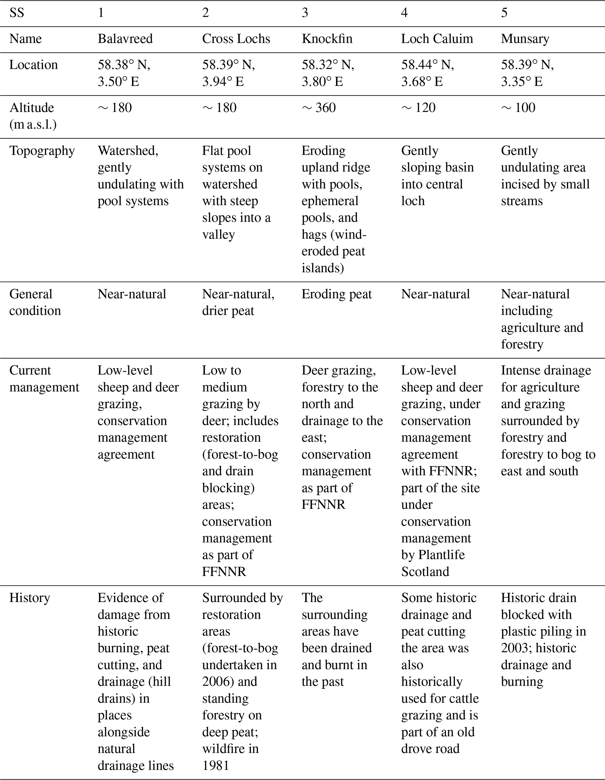
The Flow Country peatlands, northern Scotland (Andersen et al., 2018), exist in a range of topographic, hydrological, and management settings, leading to a range of different conditions, e.g. highly eroded uplands to relatively intact low-lying peatland with pool systems, with activities such as forestry, drainage, and grazing superimposed. Our chosen study site is 930 km2 of blanket bog, ranging from 50 to 600 m a.s.l. (Fig. 1). From the 19th century onwards, management has involved burning to support grouse shooting, artificial drainage of the driest areas of peatland, subsidised agricultural improvement, and later afforestation programmes (Sloan et al., 2018). More recently, near-natural areas have been designated for conservation (Lindsay et al., 1988), and previously afforested and drained areas started undergoing restoration. Some areas are also actively eroding, particularly at the highest altitudes (Hancock et al., 2018). This complex mosaic of near-natural and modified peatlands makes the study site particularly suited to an investigation on the use of InSAR for mapping the peatland condition. To understand the variation and distribution in the characteristics of the APSIS-derived time series, we analysed five well-documented 10 to 15 km2 sub-sites within the study area (Table 1; Fig. 1).
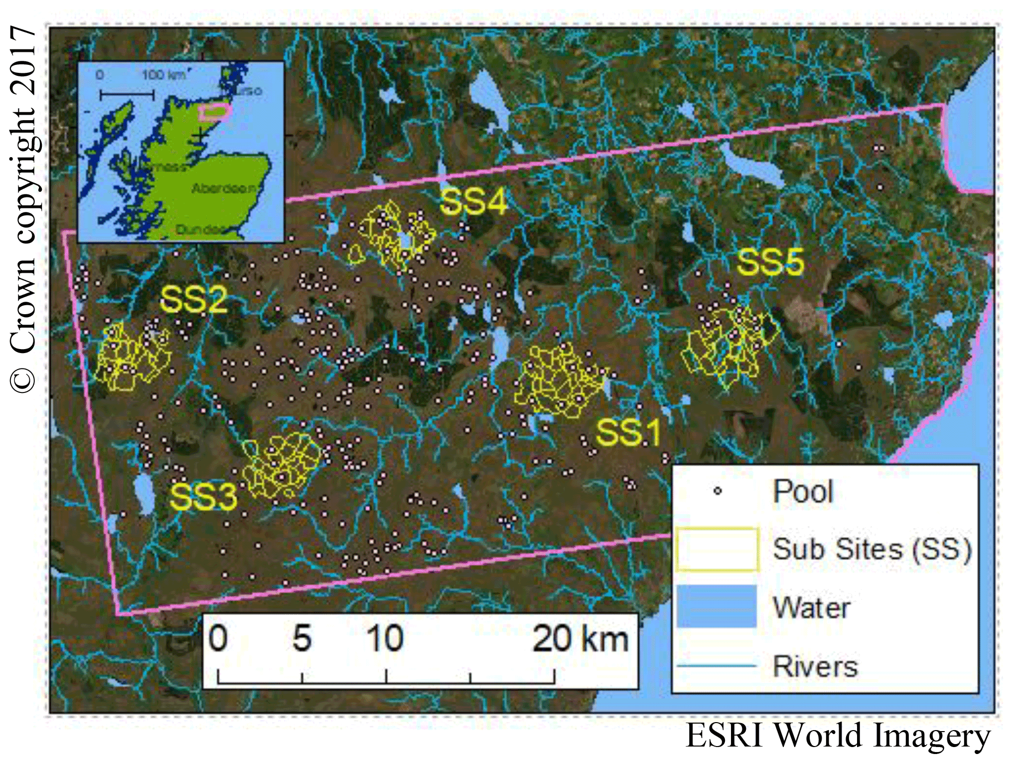
Figure 1The study location (inset) and true colour satellite image composite covering the study area, outlined, in the Flow Country, northern Scotland. Forested areas are dark green; more intensive agriculture appears as lighter greens to the north-east, with the remainder of the image mostly consisting of blanket bog. Superimposed on the image are the main river network and the location of pool features shown with sub-sites for detailed analysis marked as SS1 to SS5. Credits: Esri World Imagery; sources: ESSRI, DigitalGlobe, GeoEye, i-cubed, USDA FSA, USGS, AEX, Getmapping, Aerogrid, IGN, IGP, swisstopo, and the GIS User Community, © Crown copyright 2017. Distributed under the Open Government Licence (OGL). Ordnance Survey (Digimap Licence).
Table 1Details of the five sub-sites (SSs), which are all currently designated Site of Special Scientific Interest (SSSI), Special Protection Areas (SPA), and Special Areas of Conservation (SAC). FFNNR: Forsinard Flows National Nature Reserve.
3.1 InSAR and time series preparation
InSAR surface motion time series were calculated at a pixel resolution of 80 m × 90 m across the study site. To calculate the surface motion, we used 410 Sentinel-1A and -1B synthetic aperture radar images (descending orbit 125) gathered every 6 to 12 d between 12 March 2015 and 1 July 2019 from the European Space Agency Copernicus Open Access Hub (https://scihub.copernicus.eu, last access: 18 March 2022). Satellite interferometry was applied using these images with the APSIS technique (Sowter et al., 2013). The APSIS technique contains an adapted version of the established SBAS Differential InSAR time series algorithm (Bateson et al., 2015; Cigna and Sowter, 2017). It was designed to improve the density and spatial distribution of survey points to return measurements in vegetated areas, where Differential InSAR processing algorithms habitually struggle due to incoherence (Osmanoğlu et al., 2016; Gong et al., 2016). The APSIS algorithm was implemented using Terra Motion Limited's in-house Punnet software, which covers all aspects of processing from the co-registration of SLC (Single Look Complex) data to the generation of time series (Sowter et al., 2016). Standard interferometry image thresholds were as follows: a maximum horizontal baseline no more than 250 m, a maximum temporal separation of 1 year between image pairs using a coherence threshold of 0.25, and a minimum multi-look point acceptance threshold of 360 to a resolution of 80 m by 90 m. Motion was measured relative to a stable reference point, a building on glacial till, at Wick Airport (58.4533∘ N, 3.0879∘ W). Phase unwrapping was implemented using an in-house implementation of the Statistical-cost, Network-flow Algorithm for Phase Unwrapping (SNAPHU; Chen and Zebker, 2001). Two products were produced for each georeferenced pixel location, the multi-annual average velocity (m yr−1) of the time series calculated from the radar line of sight, and the 6–12 d time series of surface motion that detects the seasonal expansion and contraction (or bog breathing) as annual oscillations in relative height (Alshammari, et al., 2018). Each motion time series was then processed as follows.
First, using the R programming environment (R Core Team, 2013), the time series was sub-sampled into equal time intervals of 12 d, to match the longest overpass interval of Sentinel-1 images since Sentinel-1B, which reduces overpass times to 6 d, was not operational until 2016. Outliers were re-estimated using the R “tsclean” function (Box and Cox, 1964), from the R package “Forecast” (Hyndman et al., 2019). Gaps were filled with a linear interpolation using the R “approx” function (Becker et al., 1988) from the R “stats” package (R Core Team, 2020) after “spline” interpolation methods were found to produce contradictory results with adjacent time series across the largest gaps. The “detrend” R function aligned and reset each time series around zero by subtracting the mean.
Second, multichannel singular spectrum analysis (MSSA) using the SSA-MTM toolkit (Ghil et al., 2002; SPECTRA, 2021) was applied to isolate the cyclical, annual seasonal component of the time series from regional climate trends. The MSSA procedure initially calculates covariance after channel reduction with principal component analysis (PCA); then, using moving windows of 2–12 months, long enough to capture annual cycles, we recovered 80% of the signal variance in the first 20 empirical orthogonal functions (EOFs), which included the seasonal cycles in the time series. In the first instance, surface motion time series were reconstructed using EOFs 1–6. This reconstruction captured the seasonal cycles but also included longer-term climate trends, notably 3 wetter years leading to the 2018 European-wide drought (Buras et al., 2020). This climate trend causes merging and shouldering of peaks that compromised the detection of the seasonal cycles, particularly in the west of the study area, where it is wetter. To overcome this difficulty, we used a surface motion time series reconstruction using EOFs 5 and 6 (Fig. 2; Sect 1.1 and Fig. S1 in the Supplement) which extracted only the seasonal cycles. The final MSSA reconstruction provides a signal of relative movement, not absolute surface height, where a rise in the bog surface is an increase in displacement values and a fall is a decrease (Fig. 2).
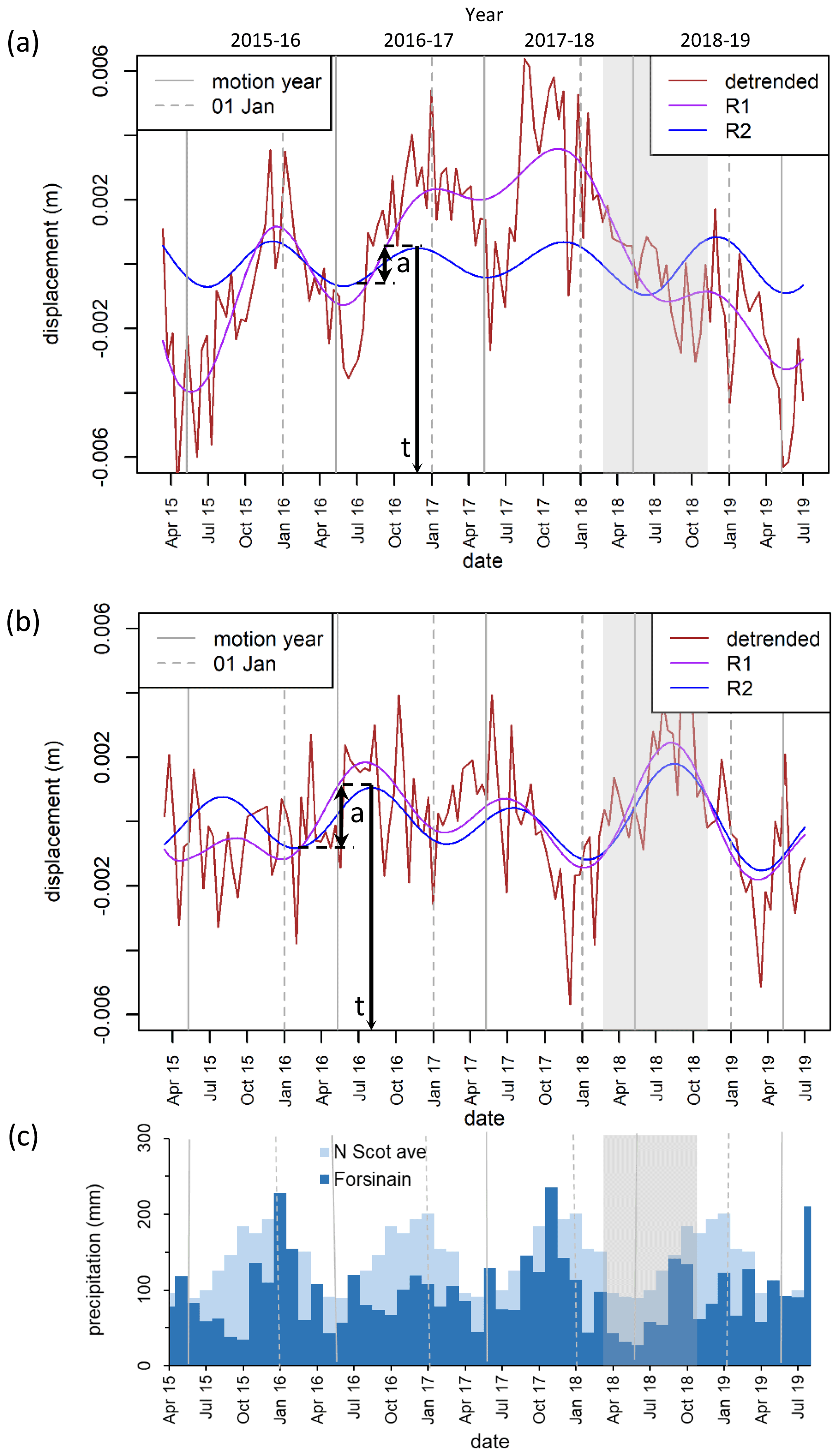
Figure 2Examples of surface motion time series and the metric definitions for (a) “soft” wet bog and (b) a “stiff” drier bog, calculated from Sentinel-1 APSIS InSAR time series data between 12 March 2015 and 1 July 2019 against (c) monthly precipitation for northern Scotland (UK Met Office 20-year average, light blue) and Forsinain in the Flow Country (Scottish Environment Protection Agency, Dark blue). The initial mean detrended time series (brown), and multichannel singular spectrum analysis (MSSA) reconstructions (R1) retaining the local climate trend (purple, a combination of empirical orthogonal functions 1–6) and R2 annual seasonal cycles (blue, a combination of empirical orthogonal functions 5 and 6) are shown. The two surface motion metrics used in the analysis are peak timing (t) and amplitude (a) shown for the surface motion year 10 May 2016 to 9 May 2017. A third surface motion metric, multi-annual average velocity, is not illustrated here as it is part of the InSAR data processing (Sect. 3.1). This asynchronous timing of peaks between (a) and (b) forms a bimodal distribution in the peak amplitude timing of the peatland landscape. The drought event of 2018 (Buras et al., 2020) is shaded and can be seen to influence relative surface motion with a local climate trend in the soft, wet bog (a).
Third, the MSSA reconstructions were then analysed for two of three surface motion metrics used to represent the condition of the peatland within each pixel for each motion year using the R “pracma” peak-find function (R Core Team, 2013). Metric one is the date of the annual peak “swelling” in the seasonal cycle (peak timing) of the MSSA reconstruction within 12 months from mid-May (Fig. 2). This has been shown to relate to peatland ecohydrology (Alshammari, et al., 2020; Tampuu et al., 2020). Metric two is the annual maximum amplitude (m) in the surface motion signal (amplitude) measured from the previous minimum of the MSSA reconstruction (Fig. 2). This is an indicator of the elastic response of the peat to changes in water storage (Roulet, 1991; Waddington et al., 2010). Metric three is the multi-annual average velocity (m yr−1) of the peatland surface calculated directly and previously described from the APSIS processing. This is a measure of vertical peatland growth (greater positive value) or subsidence (greater negative value) calculated over a fixed section of the time series (Sowter et al., 2013).
As the 2018 drought caused severe and widespread subsidence, it was found to have subdued the multi-annual average velocity and for this reason, we concentrated our analysis between 10 May 2015 and 9 May 2018, discarding the drought period. Multi-annual average velocity was recalculated accordingly. While the impacts of climate anomalies on the time series were noticeable and interesting, the first step is to gain an understanding of how InSAR data can be used to characterise peatland condition, and we focus on this aspect. We also screened time series with multiple peaks per annum or years where peaks were not discernible, and these pixels were classed as having irregular cycles. Irregular time series made up 8.4 % of the data set and are commonly associated with water courses and damaged bog (including agriculture and some forested pixels). Exclusion of these irregular time series does not affect our conclusions. Additionally, for the first year in the time series (2015 to 2016) many surface motion time series are truncated preventing the accurate calculation of amplitude or peak timing. In that year the mapping is incomplete, so for clarity we show results for a complete motion year from the mid-section of the concentrated analysis (2016 to 2017). To understand the relationships between the three metrics with respect to peatland condition we visualised the metrics in a three-axis plot (Fig. 3).

Figure 3Characteristics of the motion metrics by sub-site (SS) calculated from MSSA reconstructions of the InSAR-detected annual motion between 10 May 2016 to 9 May 2017. (a) Frequency of peak timing throughout the motion year, where May is the period of least surface motion activity, with a binomial distribution split at 10 November into an early (blue) and late (green) cluster. (b–f) Three-axis plots of the surface motion metrics: (b) SS1 Balavreed, (c) SS2 Cross Lochs, (d) SS3 Knockfin Heights, (e) SS4 Loch Caluim, (f) SS5 Munsary. Axis: x, peak time (Month); y, amplitude (Amp.: m), z, multi-annual average velocity (Vel.: m yr−1). For multi-annual average velocity, greater positive is peatland growth and greater negative is peatland subsidence. Magenta box is for visual reference. Each sub-site demonstrates a specific range in peatland condition according to the plot space it occupies.
3.2 Ecohydrological classification of the sub-sites
The training bed of the sub-sites SS1 to SS5 was divided manually into 130 smaller polygons (hereafter, sub-site polygons). Polygons ranged from (0.3 to 0.6 km2), a practical size (a) for reliable field and map-based validation and (b) to be appropriate for capturing key features of the landscape (e.g. pool systems, forestry or restoration blocks, streams and banks). To find boundaries between the polygons, one of the authors without specialist peatland knowledge searched for distinct contrasts in the landscape structure (e.g. topographic setting, natural drainage, evidence of drainage ditches and where these features would influence hydrology, forestry plantation, restoration, land management and the likely range, consistency or inconsistency in peak timing). This was possible using Google Earth, maps and the InSAR data (Supplement 1.2, Fig. S2). An additional set of 125 polygons was randomly selected across the whole study area using the Esri ArcMap “random point” tool (hereafter, random polygons). The immediate area close to the point were similarly assessed for features in the landscape, to define the polygon boundaries (most between 0.2–0.5 km2). While the sub-sites included the continuum of conditions and features adjacent to each other, the random polygons ensured that there was an improved capture of the ecohydrological states across the whole study area, reducing the likelihood that the sub-sites may have excluded a particular ecohydrological state. Summary statistics of the three surface motion metrics were calculated for each polygon. Average altitude, slope and aspect for all InSAR points in each polygon were also calculated from the Shuttle Radar Topography Mission Digital Elevation Model (Jarvis et al., 2008) to provide measures of topography (Supplement 1.3).
The full set of polygons (sub-sites and random polygons) was then passed to one of the authors with specialist peatland knowledge and based locally for a “blind” (i.e. without prior knowledge of or information about InSAR metrics within the polygons) ground-based ecohydrological classification. For each polygon, the cover of plant functional types (PFTs; Sphagnum, other mosses, shrub, sedges, grasses, rushes, and conifer trees) and the presence of hydrological features (pools, streams, drains, erosion gullies, slope) were recorded using a semi-quantitative scale (0: not present or scarce; 1: present; 2: co-dominant; 3: dominant). Current management (conservation, drainage for agriculture and peat cutting, forestry, restoration by forest-to-bog, restoration by drain blocking, and wind-farm construction) and historical management (e.g. burning, land-use conversion including wind-farm development, and restoration) were also documented for each polygon. The author responsible for classification visited and surveyed all the sub-site polygons and 86 of the random polygons (i.e. 85 % of all polygons) by walking across the area within the mapped polygon. For the random polygons where access was not permitted, shared local knowledge from stakeholders (land managers, project officers on the ground, wardens, and gamekeepers) was used instead of a field visit. In all cases, this was complemented with a combination of existing data, 1:50 000 UK Ordnance Survey maps, NatureScot National Vegetation Classification maps (SNH, 2019), and Google Earth imagery.
Using the semi-quantitative scores, the PFT and hydrology polygon attributes were clustered by similarity using a hierarchical cluster analysis (HCA; Supplement 1.4, Fig. S3). To avoid an overly split hierarchical tree with only one or two members per cluster requiring complex explanation, it was deemed more informative to analyse the PFTs, hydrology, and the topography categories separately from each other. For the PFTs, once the clustering was complete, the average score of the semi-quantitative scale of each PFT in the cluster was ranked. The top three PFTs were used to characterise and name the plant functional group composition (Tables S1–S4 in the Supplement). For data visualisation of the results, clusters were further grouped based on the dominant PFT, resulting in five plant functional groups: Sphagnum, shrub, grass, bare peat (where low or absent vegetation was dominant), and forestry (Table 2). The four polygons that were dominated by rushes (R) had shrub as a co-dominant vegetation, so they were incorporated into the shrub group. While sedges (Sg) were co-dominant in many Sphagnum and shrub polygons, they were not the dominant PFT in any cluster and therefore did not form a separate group.
Table 2Percentage proportion of clusters derived from hierarchical cluster analysis based on plant functional types (PFTs) represented in the polygons of the five sub-sites and the random polygons. Clusters are defined by the dominant (first) and co-dominant (subsequent) PFTs. PFT notations: Sp – Sphagnum; S – shrub; Sg – sedges; M – moss; G – grasses; R – rushes; F – forest; LoA – low or absent vegetation (brash, bare peat following tree felling or restoration activities, etc.). n: number of polygons. For data visualisation, the sub-site and random clusters were then grouped into five plant functional groups based on the dominant PFTs: Sphagnum, shrub, grass and rushes, bare peat, and forestry. Clusters dominated by rushes (R) were incorporated into the shrub group for data visualisation given their low number and shrub co-dominance. Bare peat and forestry were retained despite low numbers, as their vegetation is associated with specific management intervention. Footnotes describe further differences between clusters (Tables S2 and S4).
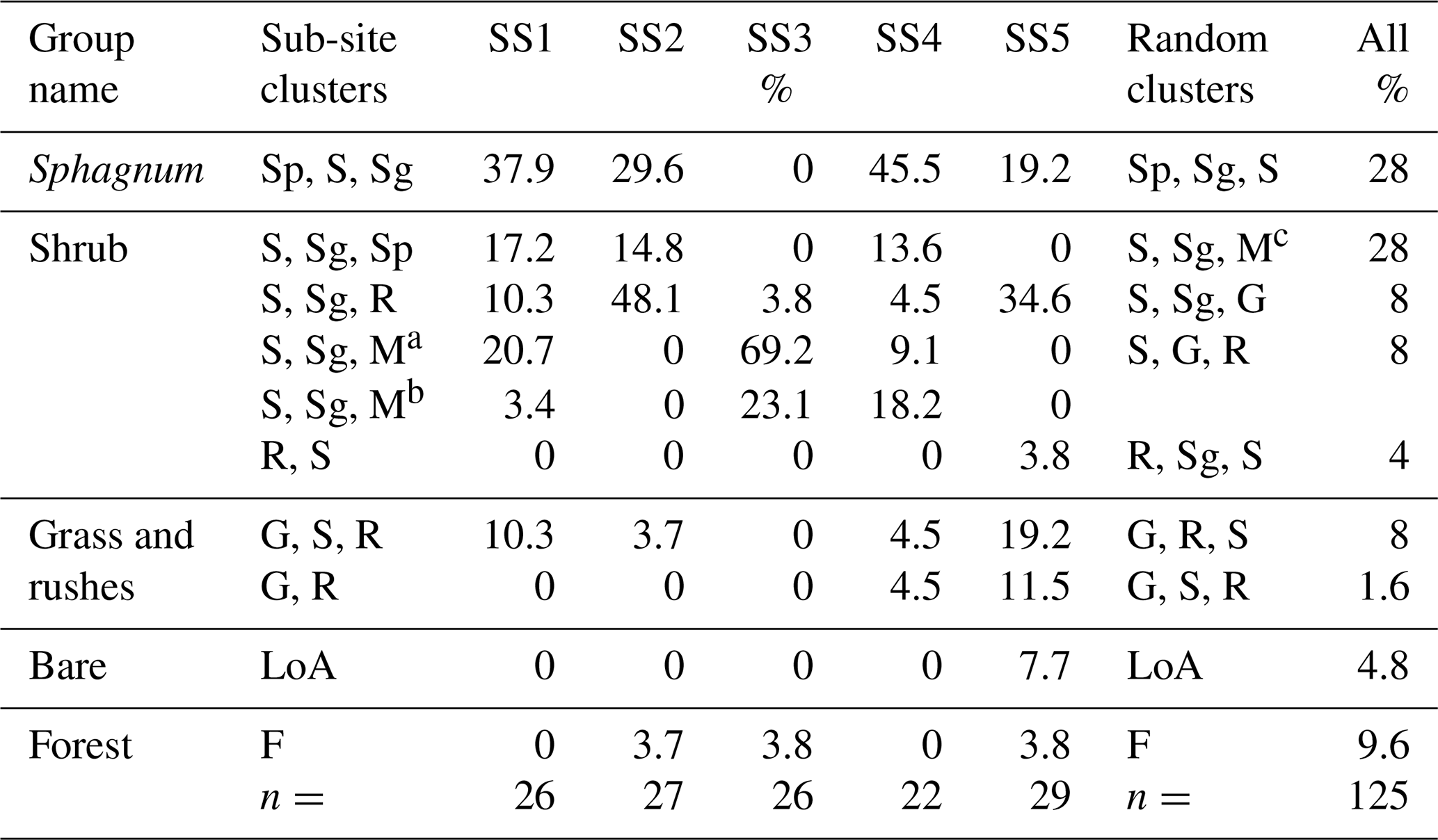
a Additional presence of G. b Additional presence of R. c Absence of G.
We also categorised topography into equal altitude belts (0–150, 151–300, and 301–450 m) and split slope face direction into four quadrants (north, east, south, and west facing) and ran the HCA. Except for the highest most eroded SS3 site, altitude and aspect did not show any meaningful cluster groups and played no further part in the analysis. The lack of topographic relationships is largely due to the gentle relief of the Flow Country, which has few sheltered slopes and deep valleys. Instead, we used average gradient (degrees) in the polygon and found a natural breakpoint at 1.5∘ that split the data set equally between flat (<1.5∘) and slope (>1.5∘).
3.3 Mapping the state of the peatland system
Within the three-axis plot, we then chose a point with a winter peak timing, a high amplitude, and extreme positive velocity, normally associated with “soft”, wet Sphagnum peat and mapped the whole study area relative to that point. The actual reference point was selected by isolating the points that peaked in the winter and then stepping down through the percentiles of the metrics distributions until the case with the most frequent timing (e.g. February), highest positive velocity (e.g. 0.006 m yr−1), and highest amplitude (e.g. 0.008 m) was identified. For the condition mapping, data for all other points in the three-axis plot were then paired with this reference point and the Euclidian distance between them in three-dimensional (Cartesian) space was calculated. Based on the subsequently observed bimodal distributions (Sect. 4; Fig. 3), if the paired point was on the opposite side of the bimodal distribution to the reference point, the Euclidian distance was mapped as a “V”-shaped path via zero velocity and zero amplitude at the mid-date, 10 November, between the earlier and later timed clusters in the distribution. Prior to calculation, the positions of the outer portions of the three-axis plot were adjusted. This is because if the paired point is before (left of) the earlier peak and after (right of) the later peak the difference between the peak timing and the origin would be overestimated. To mitigate this, these cases were folded inwards along the axis of the peak of their distributions (effectively turning the upturned “W” shape of the bimodal distribution into an “M” shape). Using the natural breaks (Jenks) classification in Esri ArcGIS as a guide, thresholds were used to classify distance from the soft, wet Sphagnum point. These values were then mapped to produce an ecohydrological classification across the whole study site.
To further validate our ecohydrological classification map, we remotely identified and marked the central locations of all the pool systems within the study area (328 in total) using Google Earth images and determined if these markers corresponded to the soft, wet Sphagnum state. Although soft, wet areas in which Sphagnum is dominant do not necessarily contain pool systems, pool systems in this area almost always contain soft, wet peat. Furthermore, in the study area, pool systems provide a spatially distributed, abundant, and easily identifiable sample of this part of the peatland system. They also correspond to the part of peatland systems most unequivocally associated with the “near-natural” ecohydrological condition in this type of upland blanket bog. As the position of each pool marker did not take into account that pool systems often display complex morphology and varying geometries (and sometimes variable condition) related to local hydrological conditions (Goode, 1973; Lindsay, 2018), there was a need to tolerate a level of spatial uncertainty. To capture this, a wider area of 150 m (using the buffer function in Esri ArcMap) was calculated around the marker. This buffer area contained at least three pixels by three pixels of the ecohydrological map. We then calculated the percentage of pixels identified in the ecohydrological classification as soft in the buffer. Pixels classed as irregular were not included in the count (Table S5). We acknowledge that we focus on one particular state of peat, which does not account for the presence of drier, thin, or damaged peat conditions. Indeed, stiffer, thin, and damaged peat cannot readily be associated with a single, well-defined and remotely identifiable feature distributed across the whole study area in the same way. For instance, whilst drains can be observed from Google Earth, their age, maintenance, and the extent of their impact on the peat would require further evidence beyond the scope of this study.
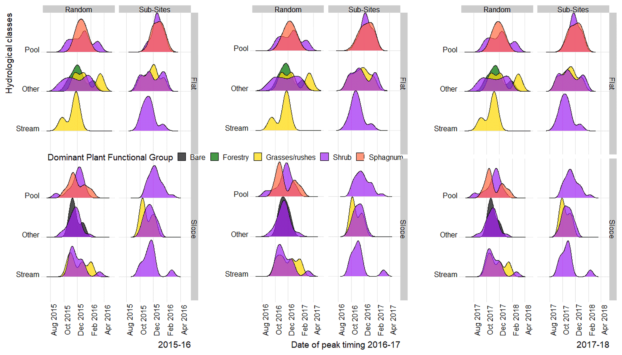
Figure 4Distribution of mean peak timing date by dominant plant functional clusters for polygons with pools, streams, or other hydrological features (e.g. drains, erosion gullies, peat cutting, or no apparent features) in either a flat (gradient < 1.5∘) or slope (gradient > 1.5∘) topographic setting for the random and sub-site polygons. Plant functional group polygons (n random/sub-site): bare – bare peat (); forestry – conifer plantation (); grasses and rushes – grass-dominated communities (), typically Molinia caerulea; shrub – shrub-dominated communities (), typically either or both of Calluna vulgaris and Erica tetralix; Sphagnum – Sphagnum-dominated communities . Sedges, rushes, and other mosses are also present, often as co-dominant species in both Sphagnum and shrub communities (see Table 2).
From the frequency histograms of maximum peak timing, we discovered a bimodal distribution, showing an early and late peak (Fig. 3a) and defined the motion year to begin at the least active swelling period on 10 May to avoid dividing periods of maximum swelling into consecutive calendar years. The bimodal distribution peaks fall between August to October and December to February, similarly illustrated in the three-axis plots (Fig. 3b–f). For each of the sub-sites, the plots of the three motion metrics show small variations in the shape and position of the data cluster reflecting the diversity of peatland conditions sampled across the landscape.
4.1 Relationship between surface motion and ecohydrology
The HCA revealed ecological groups relating to dominant plant functional types that were comparable between the sub-site and random polygons (Table 2) as well as hydrological groups separating polygons with pool systems and polygons with streams from all other polygons (Fig. S3). When the HCA classifications and topographic information (slope) were compared to the surface motion metrics, we determined the following consistent relationships for the sub-site and random-site polygons.
4.1.1 Timing, hydrology, and topography
Shifts in the peak timing distributions relate to a combination of topography, hydrology, and plant functional group (Fig. 4), and peak timings themselves were consistent within groups between the 3 motion years. Sphagnum-dominated polygons are almost exclusively associated with pools and more so on flat ground with a tendency to have a peak later in the year than most other hydrological and topographical combinations of vegetation or hydrological features. Within the hydrological class pool, polygons with topographic gradients greater than 1.5∘ (slope) for both random and sub-site polygons have their highest peak timing frequencies earlier in September and October than polygons with topographic gradients less than 1.5∘ (flat), which tend to peak in November, January, and February. The steeper gradients, at both random and sub-sites, tend to be associated with shrubs and grass-dominated vegetation communities with low frequencies of Sphagnum-dominated polygons. Polygons with pools as the dominant hydrological feature tend to have their highest frequencies from October onwards, later than polygons classed as stream or polygons with other features (drainage ditches, peat cutting, or erosion gullies).
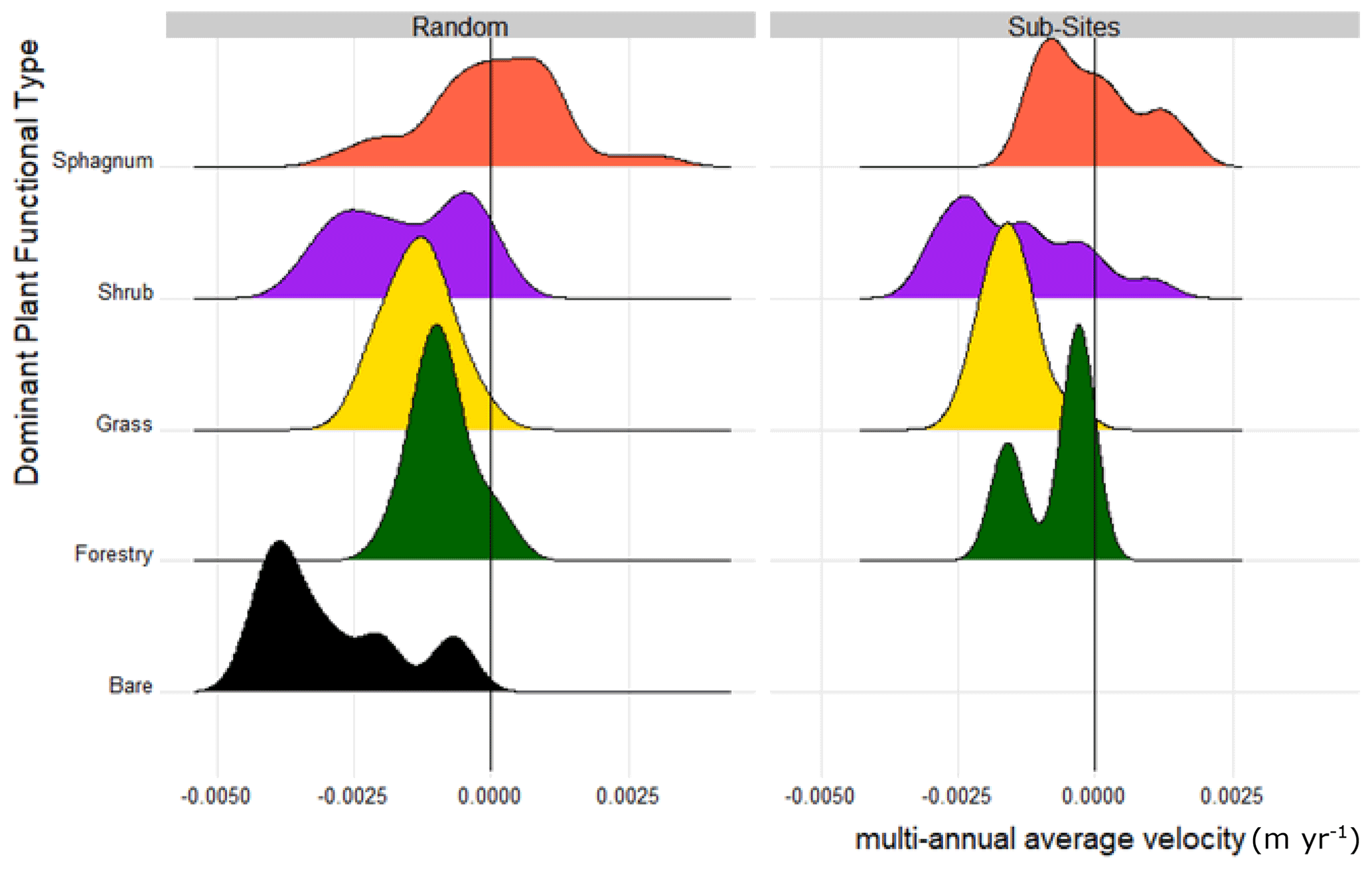
Figure 5Distribution density of multi-annual velocity for each plant functional group and polygon type plant functional polygons n (random/sub-site): bare – bare peat (); forestry – conifer plantation (); grasses and rushes – grass-dominated communities (); typically Molinia caerulea; shrub – shrub-dominated communities (), typically either or both of Calluna vulgaris and Erica tetralix; Sphagnum – Sphagnum-dominated communities . Sedges, rushes, and other mosses are also present, often as co-dominant species in both Sphagnum and shrub communities (see Table 2).
4.1.2 Multi-annual average velocity and dominant plant functional group
Multi-annual average velocities that were most positive (gain of height over time) were almost entirely dominated by Sphagnum (Fig. 5). Polygons with plant functional groups typically associated with natural or man-made drainage (shrub), disturbance (forestry and bare peat), or thin, degraded peat (grasses) consistently displayed negative long-term multi-annual average velocities (loss of mass over time) regardless of topographical setting. Sites in which grasses or forest dominate tend to have a more intermediate multi-annual average velocity than either shrub- or Sphagnum-dominant polygons. Where bare peat is dominant, multi-annual average velocities are lowest (most negative).
4.1.3 Multi-annual average velocity and management
When multi-annual average velocities are compared across different management classes (Fig. 6), the least negative values are observed under conservation management and most negative values are associated with forest-to-bog management, a restoration approach that typically involves compaction from heavy machinery during the removal of conifer stands, followed by drain blocking and surface re-profiling. This restoration class shows a broader distribution in long-term multi-annual average velocity than other management classes, reflecting a variable degree of recovery associated with differing starting conditions, time since initiation (ranging from 0 to >15 years), and techniques used in the intervention.
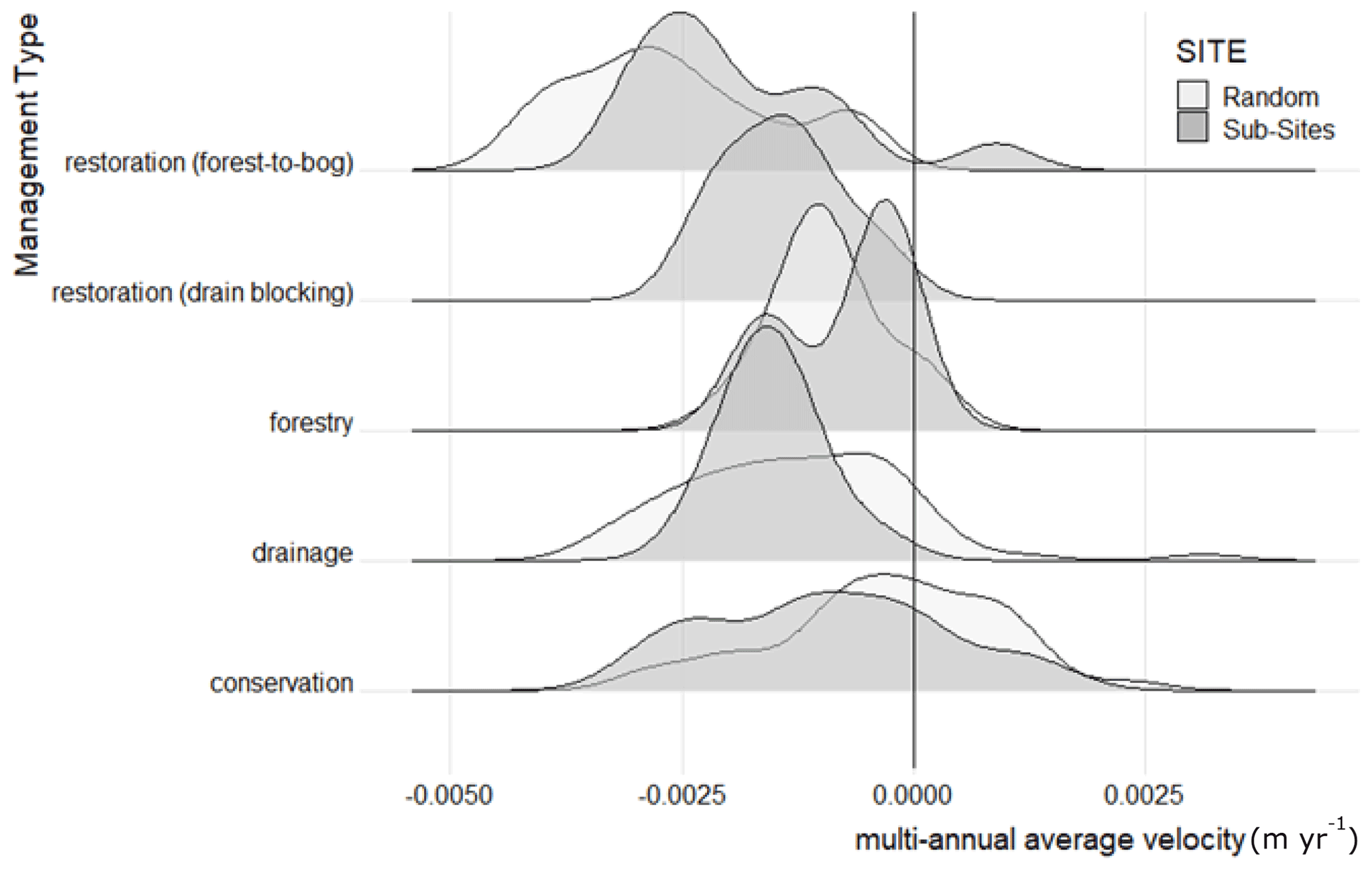
Figure 6Distribution density of multi-annual average velocity for different management groups and by polygon type (sub-site and random). Management polygons n (random/sub-site): restoration (forest-to-bog) , restoration (drain blocking) , forestry , drainage , conservation .
4.1.4 Time and magnitude of peatland swelling
The factors that influence amplitude can be deduced from relative annual amplitude change and peak timing plots for the three most dominant PFT clusters (Sphagnum, shrub, and grass) across 3 surface motion years (Fig. 7). These graphs all show a positive trend between timing (day of year) and amplitude with a tendency for higher amplitudes to usually occur later in each surface motion year. Steeper slopes tend to have the lower amplitudes that peak earlier in the surface motion year. Shallow to flat slopes tend to have higher amplitudes and peak later in the surface motion year. Year-on-year variation in the range of observed amplitudes is apparent, with a large range in 2015–2016 and smaller ranges in the 2 subsequent years. We attribute this to interannual variation and antecedent conditions in rainfall (e.g. Fig. 2c). A relatively dry 2014–2015 resulted in a strong amplitude response in 2015–2016 with lesser responses in the 2 subsequent wetter years. These differences can be related to the amount of unfilled pore space in the uppermost layer of the peat. In essence, as the peat gets wetter and the pore space fills, there is less capacity in the peat to add more water and the amplitude response diminishes. A more saturated state of the peatland in 2016–2017 and 2017–2018 was also noted in field observations.
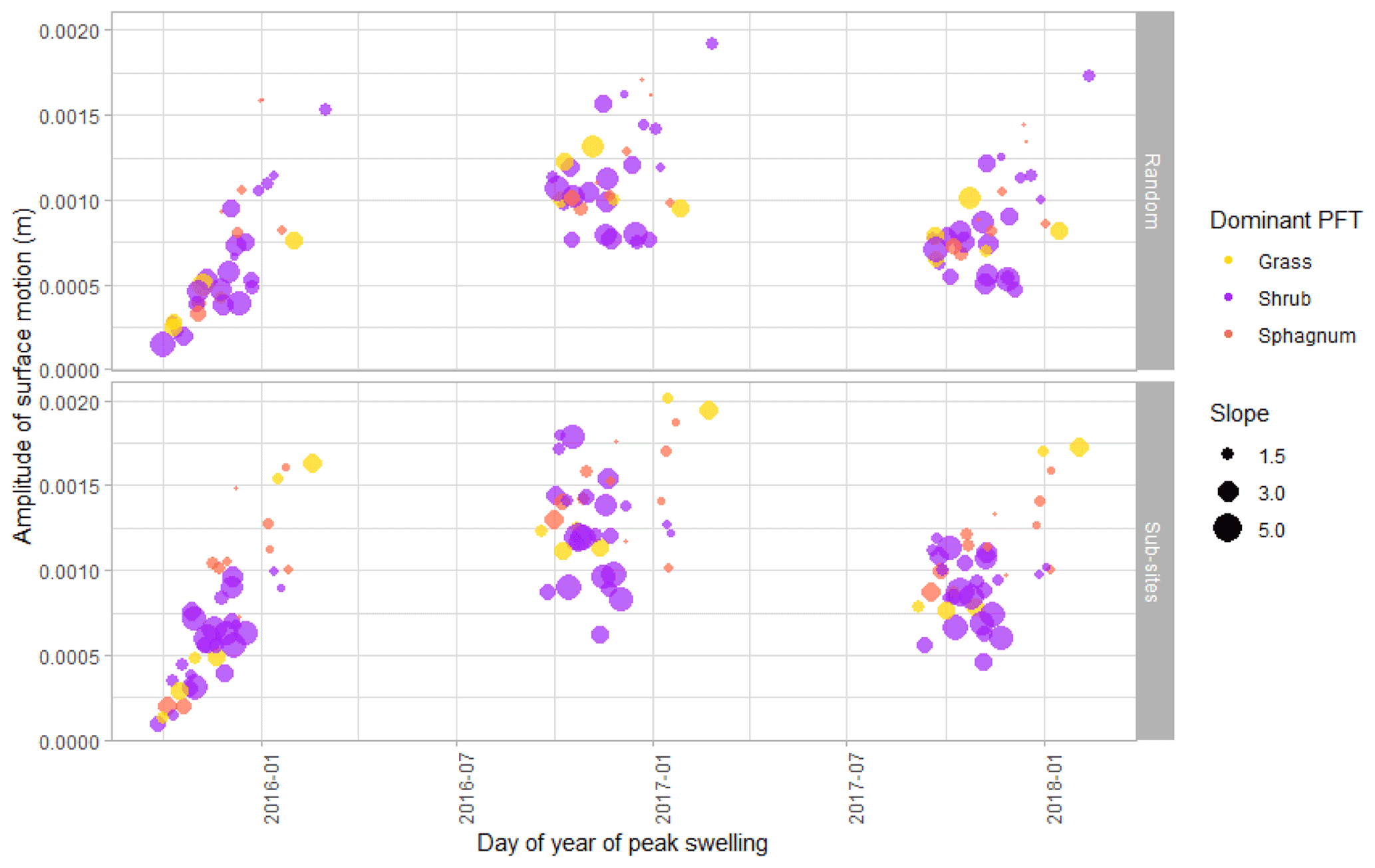
Figure 7Timing of and relative amplitude for 3 consecutive years (2015–2018) with respect to slope gradient (degrees), dominant plant functional type (PFT; grass, shrub, and Sphagnum), and polygon type (sub-site and random).
4.2 Application to large-area condition mapping
The observed relationship between surface motion metrics and ecohydrology is readily interpreted in the context of reported field measurements of peat surface motion (Howie and Hebda, 2018; Morton and Heinemeyer, 2019). Flatter sites under near-natural conditions are poorly drained, wetter, and dominated by Sphagnum spp. In turn, Sphagnum spp. have a considerable capacity for water storage as a direct result of their physiology (Kellner and Halldin, 2002), resulting in peak water storage and seasonal swelling of the surface later in the year. Drier sites with compacted peat have less capacity to store water and reach water holding capacity earlier in the autumn (Price, 2003). Furthermore, the more degraded peat at these sites is less elastic and therefore exhibits a lower-amplitude response to changes in water storage (Holden et al., 2004; Lui and Lennartz, 2019). As the seasonal water balance shifts, drier, better drained sites lose water first followed by the Sphagnum sites, which may continue to swell on account of hysteresis during the first stages of water loss (Howie and Hebda, 2018). Synthesising Sect. 4.2 (Figs. 4–7) the bimodal distribution of peatland surface motion timing within our landscape may be interpreted as reflecting two dominant components of the landscape. Wetter, flatter sites, typically dominated by Sphagnum and sedges, are soft peats; they tend to reach peak surface heights later in the year (December to February window) and have higher amplitudes and more positive velocities. Drier shrub- and grass-dominated sites are “stiff” peats; they tend to reach peak surface heights earlier in the year (August to October window), with slightly (but not exclusively) lower-amplitude oscillations and more negative velocities. Additionally, in the three-axis plot there are points characterised by both low amplitudes, negative velocities, and peak timings that can also fall outside the window of the soft and stiff class. These subtle variations in the metrics identified a third broad ecohydrological class which reflects thin peats, the most degraded and drained grass-dominated sites, or sites under restoration that are in transition to either a soft or stiff state.
Mapping and applying thresholds to the Euclidian distance calculations into these three broad peatland classes relative to the soft peat condition generated the peatland condition map (Fig. 8a). The classification produced a patchwork of conditions in the Flow Country, and the map evidences the widespread occurrence of the stiff peat condition associated with both naturally drier areas on the slopes and wet, soft peat margins but also areas made drier by a land-use history of burning and drainage. The impact of restoration activities, following the felling of forestry on deep peat in the last 25 years, can also be seen: recent forest-to-bog clearance is displayed as “thin/modified” peat, whilst areas well on their way to recovery are showing as either the soft or stiff condition (Fig. 8b and c). In polygons where forest is planted on peat, the signal is much more mixed with a greater proportion of the irregular class. This mixture is a result of the poorer SAR response over trees and the variable conditions encountered within forest stands. For example, in these forestry plantations, fire breaks, gaps between blocks (termed “rides”) and riparian areas that were never planted can still be wet, soft, and Sphagnum-rich in contrast with the planted blocks themselves. Furthermore, plantations may enclose areas of deep peat with pools and may display variable wetness and dryness depending on site and topography.
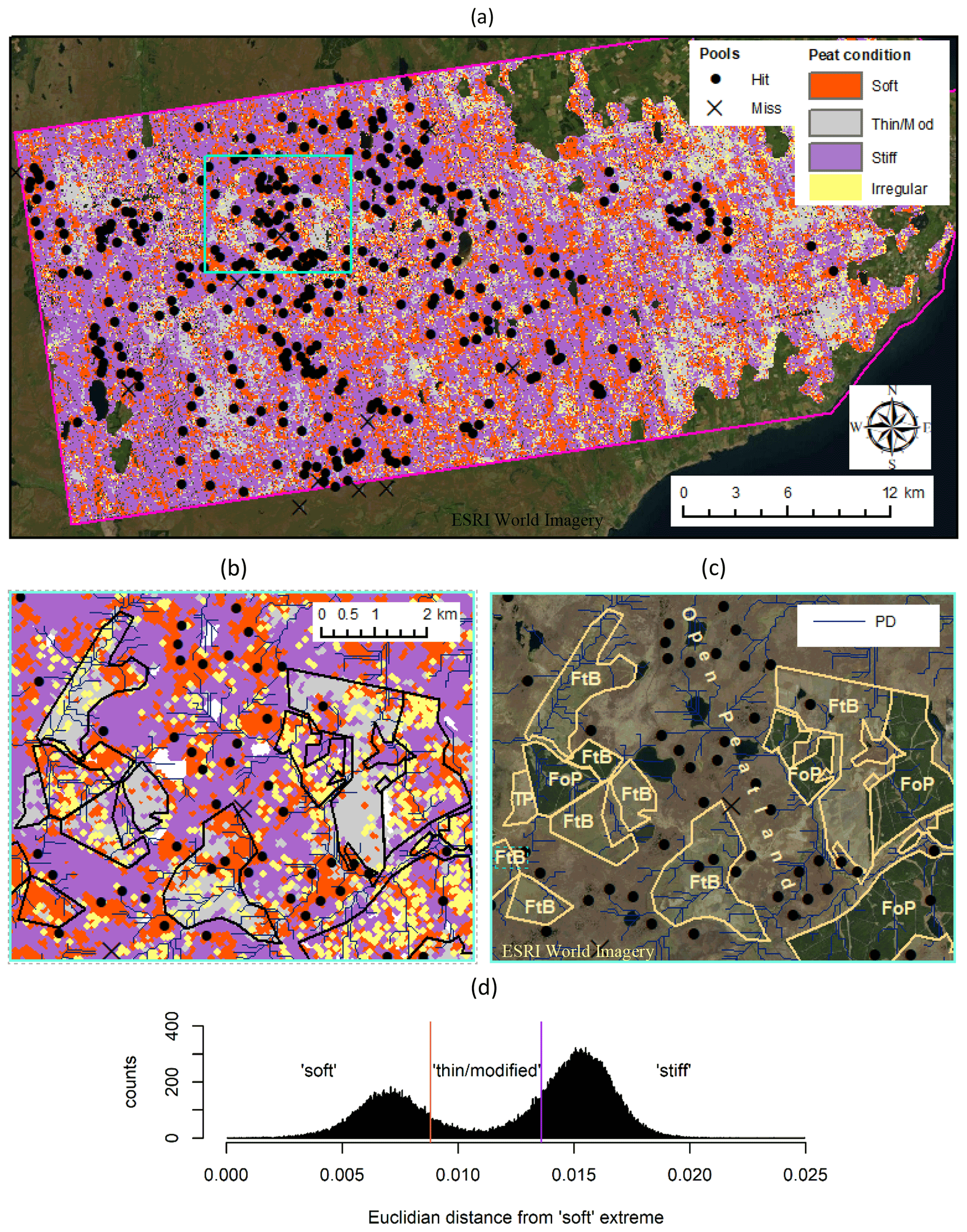
Figure 8The ecohydrological classification of “soft”, “thin/modified”, and “stiff” peatland condition, with respect to the location of pool systems, and areas of forest-to-bog restoration in the study area. (a) Classified map based on the Euclidian distance (in three-dimensional Cartesian space) from the position of the soft reference to all other points in the three-axis plot of peak timing, amplitude, and multi-annual average velocity, including the screened irregular time series for the period 10 May 2016 to 9 May 2017. Pool systems that have been correctly classified are shown as a “hit” and otherwise as a “miss”. (b) A detailed view of the classified area highlighted within (a) illustrating the relationship with hydrology, determined from a DEM (potential drainage, PD) and polygons delineating areas for restoration. (c) A true colour satellite image of area showing the restoration status of the polygons, un-felled forest on peat (FoP), peat areas at various stages or different years of forest-to-bog (FtB) restoration, and an area of thin peat (TP). (d) Frequency distribution of Euclidian distance, and the thresholds used to differentiate between the three peat conditions. Credits: the classified area (approx. 930 km2) was delineated using peat soils from the National Soil Map of Scotland (JHI, 2021). Images sourced via Esri ArcMap in 2021. Image source for (a) and (c) Esri World Imagery: Esri, DigitalGlobe, GeoEye, i-cubed, USDA FSA, USGS, AEX, Getmapping, Aerogrid, IGN, IGP, swisstopo, and the GIS User Community.
Using the criteria for the remote validation that pool systems should always include a pixel of the soft peat category within the 150 m buffer, 97.9 % () of the pool systems were identified as having at least one pixel of that class in the surrounding buffer (Table S5). A detailed inspection of the remaining 2.1 % () of pool system markers without a soft classified pixel within the 150 m buffer reveals that these pool systems all showed evidence of localised erosion or drainage causing degradation of their natural hydrology. While not validated in the same way, further inspection of our classification combined with specialist knowledge of the area indicates that the thin/modified class corresponds to areas under restoration, notably areas recently felled for forest-to-bog restoration, areas subject to intensive grazing, and thin peat soils on steeper higher ground and in valley bottoms (e.g. Fig. 8b and c). The abundance of the thin/modified class is striking in the east of the study area, and we note that this corresponds to long-term historical usage of the land for agriculture and associated cutting of peat for fuel (Andersen et al., 2018; Minasny et al., 2019).
Within the area, our method identifies approximately 254 km2 (27.3 % of the area) as soft, wet Sphagnum-dominated peat, 481 km2 (51.7 %) as stiff shrub-dominated peat, 117 km2 (12.8 %) as the thin/modified peat class, and 78 km2 (8.4 %) as irregular time series. This classification therefore provides an overall measure of the current state of this blanket bog landscape, to which future regional change, on account of climate change or restoration, may be compared.
Our most important finding is that surface motion metrics derived from APSIS InSAR time series enable almost continuous spatial and temporal characterisation of peatland condition at large scales. That the SAR data can penetrate cloud cover, measure regular physical displacement of the surface, and capture a known dynamic behaviour associated with peat resilience gives this approach a significant lead over the far more challenging effort to measure peatland condition from optical reflectance data (e.g. Artz et al., 2019). This is compounded by the fact that peatland areas are often obscured by cloud (Minasny et al., 2019). A valuable exercise would be to quantify the similarities and contrasts of motion-mapped peatland condition to optical products, and we anticipate that motion data will bring different and complementary information. This may be advantageous for restoration monitoring, and information on peatland mechanical condition from surface motion may be key to resolving weaknesses in optical studies, for example in carbon accounting (Couwenberg et al., 2011).
The sensitivity and dynamic response of surface motion metrics to changes in the state of the peatland system should make the method ideally suited to monitoring and informing peatland management and restoration. Globally, large areas of northern peatlands degraded by historic drainage, grazing, and forestry are now under or targeted for restoration (Rochefort and Andersen, 2017). Consequently, peatland conservation and restoration are increasingly perceived as critical tools in the fight against global climate change (Leifeld and Menichetti, 2018; Amelung et al., 2020; Günther et al., 2020). Restoration strategies typically involve raising water levels to re-establish wet conditions. The expectation is that this will promote Sphagnum establishment, often a key measure of the success of an intervention (Rochefort and Andersen, 2017; Bellamy et al., 2012; Caporn et al., 2018; González and Rochefort, 2019).
In the case of blanket bog landscapes, our finding of naturally stiff drier shrub and soft, wetter Sphagnum states raises the question as to whether a strategy of increasing Sphagnum cover is always an appropriate restoration target or indeed if it is the only desirable outcome for blanket bogs. In this context, an APSIS InSAR-based assessment of the condition of a whole blanket bog landscape can help guide restoration strategies by first identifying the typical natural states and hydrological structure of that landscape. Second, following intervention, this approach could enable a robust monitoring of restoration trajectories and outcomes (Marshall et al., 2021). Our study also suggests that when monitoring restoration trajectories over time, the impacts of interannual variabilities such as precipitation on the metrics would likely need to be accounted for.
In natural landscapes, these peatland states are a consequence of landscape evolution in which the vertical accumulation of peat must be counterbalanced on an appropriate spatial and temporal scale by erosion (Large et al., 2021). Drier states correspond to areas of net carbon loss due to natural drainage, incision, and erosion along peatland margins, and wetter states correspond to peatland interiors, areas with low gradient that tend towards carbon accumulation. In this context, to restore a site that is naturally stiff and dry to the soft, wet state would risk instability, while the opposite would fail to optimise carbon storage. A more suitable and sustainable ambition is to accept that restored blanket bog sites may follow different trajectories towards naturally Sphagnum or shrub states (or soft and stiff) and that these target end states will be constrained by the hydrological landscape setting, as conceptualised by Winter (1988). Our approach provides evidence for these natural states co-existing within the study areas and evidence to guide and monitor appropriate restoration trajectories within this system. Recognising and preserving this mosaic is critical in maintaining large- and small-scale peatland landscape stability and carbon balances, particularly as long-term models suggest that the natural drying out of peatland is accelerating due to drainage (Harris et al., 2020; Leifeld et al., 2019) and climate change (Gallego-Sala and Prentice, 2013).
The approach outlined here should be readily transferable to alternative peatland settings within different parts of the global peatland climate space. Using surface motion metrics identified from the InSAR time series of peatland motion, a surface deformation space for a given peatland system can be defined. The position of ecohydrological characteristics within this space can then be deployed to quantify the state of the peatland system and map changes with respect to climate change and management intervention. This capacity to customise the approach is valuable as it provides the means to measure peatland condition at a global scale. If realised, this would enhance our understanding of the large-scale functionality of peatland landscapes and provide the robust evidence base required for sustainable peatland management.
Data sets are available at https://doi.org/10.17639/nott.7123 (Bradley, 2021).
The supplement related to this article is available online at: https://doi.org/10.5194/esurf-10-261-2022-supplement.
AS led the processing of the InSAR data that AVB post-processed, analysed, and visualised. RA recorded the polygon attributes, mapped the pools, contributed to data visualisation, and completed the ground surveys with CM. DJL developed the overall idea of applying InSAR for this purpose. All authors were responsible for critical contributions, passing the final paper, and editing text and figures.
Andrew Sowter is affiliated with Terra Motion Limited. The APSIS (Advanced Pixel System using Intermittent SBAS) method is owned by the University of Nottingham and is the subject of a UK patent application (no. 1709525.8) with the inventor named as Dr. Andrew Sowter; it is currently patent pending.
Publisher's note: Copernicus Publications remains neutral with regard to jurisdictional claims in published maps and institutional affiliations.
We are not responsible for the consequences of any decisions or actions even if they have been influenced by the material and ideas in this paper.
The authors would like to thank members of the following organisations who provided access to sites for surveys or insight and local knowledge about past and present management over the study area: NatureScot Peatland ACTION, Royal Society for the Protection of Birds, Plantlife Scotland, Forestry and Land Scotland, Scottish Forestry, Welbeck Estate and Shurrery Estate. David Gee and Ahmed Athab are thanked for their assistance with the APSIS InSAR data output. The “National Soil Map of Scotland” copyright and database right lie with the James Hutton Institute v.1_4, and it is used with the permission of the James Hutton Institute. All rights reserved. Any public sector information contained in these data is licensed under the Open Government License v.2.0.
This research has been supported by the Natural Environment Research Council (InSAR TOPS grant no. NE/P014100/1 to David J. Large, Roxane Andersen and Chris Marshall) and the Leverhulme Trust (Leverhulme Leadership award grant no. 1466NS to Roxane Andersen and Chris Marshall).
This paper was edited by Daniella Rempe and reviewed by two anonymous referees.
Almendinger, J. C., Almendinger, J. E., and Glaser, P. H.: Topographic fluctuations in across a spring fen and raised bog in the Lost River Peatland, northern Minnesota, J. Ecol., 74, 393–401, https://doi.org/10.2307/2260263, 1986.
Alshammari, L., Large D. J., Boyd, D. S., Sowter, A., Anderson, R., Andersen, R., and Marsh, S.: Long-term peatland condition assessment via surface motion monitoring using the ISBAS DInSAR technique over the Flow Country, Scotland, Remote Sens., 10, 1–24, https://doi.org/10.3390/rs10071103, 2018.
Alshammari, L., Boyd, D. S., Sowter, A., Marshall, C., Andersen, R., Gilbert, P., Marsh, S., and Large, D. J.: Use of surface motion characteristics determined by InSAR to assess peatland condition, J. Geophys. Res.-Biogeo., 125, e2018JG004953, https://doi.org/10.1029/2018JG004953, 2020.
Amelung, W., Bossio, D., de Vries, W., Kögel-Knabner, I., Lehmann, J., Amundson, R., Bol, R., Collins, C., Lal, R., Leifeld, J., and Minasny, B.: Towards a global-scale soil climate mitigation strategy, Nat. Commun., 11, 1–10, https://doi.org/10.1038/s41467-020-18887-7, 2020.
Andersen, R., Cowie, N., Payne, R. J., and Subke, J. A.: The Flow Country peatlands of Scotland, Mires Peat, 23, 1–2, https://doi.org/10.19189/MaP.2018.OMB.381, 2018.
Artz, R. R. E., Johnson, S., Bruneau, P., Britton, A. J., Mitchell, R. J., Ross, L., Donaldson-Selby, G., Donnelly, D., Aitkenhead, M. J., Gimona, A., and Poggio, L.: The potential for modelling peatland habitat condition in Scotland using long-term MODIS data, Sci. Total Environ., 660, 429–442, 2019.
Baden, W. and Eggelsmann, R.: Der Wasserkreislauf eines nordwestdeutschen Hochmoores, in: Schriftenreihe des Kuratoriums fiir Kulturbauwesen, 12, Verleg Wasser und Boden, Hamburg, Germany, 156 pp., 1964.
Bateson, L., Cigna, F., Boon, D., and Sowter, A.: The application of the Intermittent SBAS (ISBAS) InSAR method to the South Wales Coalfield, UK, Int. J. Appl. Earth Obs. Geoinform., 34, 249–257, https://doi.org/10.1016/j.jag.2014.08.018, 2015.
Becker, R. A., Chambers, J. M., and Wilks, A. R.: The New S Language, Wadsworth & Brooks/Cole, ISBN 10 0412741504 and updated ISBN 13 9780412741500, 1988.
Bellamy, P. E., Stephen, L., Maclean, I. S., and Grant, M. C.: Response of blanket bog vegetation to drain-blocking, Appl. Veg. Sci., 15, 129–135, https://doi.org/10.1111/j.1654-109X.2011.01151.x, 2012.
Box, G. E. P. and Cox, D. R.: An Analysis of Transformations, J. R. Stat. Soc. B., 26, 211–252, 1964.
Bradley, A. V.: InSAR landscape scale peatland condition, Nottingham Research Data Management Repository, University of Nottingham, UK [data set], https://doi.org/10.17639/nott.7123, 2021.
Buras, A., Rammig, A., and Zang, C. S.: Quantifying impacts of the 2018 drought on European ecosystems in comparison to 2003, Biogeosciences, 17, 1655–1672, https://doi.org/10.5194/bg-17-1655-2020, 2020.
Caporn, S. J. M., Rosenburgh, A. E., Keightley, A. T., Hinde, S. L., Riggs, J. L., Buckler, M., and Wright, N. A.: Sphagnum restoration on degraded blanket and raised bogs in the UK using micropropagated source material: a review of progress, Mires Peat, 20, 1–17, https://doi.org/10.19189/MaP.2017.OMB.306, 2018.
Chen, C. W. and Zebker, H. A.: Two-dimensional phase unwrapping with use of statistical models for cost functions in nonlinear optimization, J. Opt. Soc. Am. A, 18, 338–351, https://doi.org/10.1364/JOSAA.18.000338, 2001.
Cigna, F. and Sowter, A.: The relationship between intermittent coherence and precision of ISBAS InSAR ground motion velocities: ERS-1/2 case studies in the UK, Remote Sens. Environ., 202, 177–198, https://doi.org/10.1016/j.rse.2017.05.016, 2017.
Couwenberg, J., Thiele, A., Tanneberger, F., Augustin, J., Bärisch, S., Dubovik, D., Liashchynskaya, N., Michaelis, D., Minke, M., Skuratovich, A., and Joosten, H.: Assessing greenhouse gas emissions from peatlands using vegetation as a proxy, Hydrobiologia, 674, 67–89, https://doi.org/10.1007/s10750-011-0729-x, 2011.
Crump, J. (Ed.): Smoke on water: Countering global threats from peatland loss and degradation, UNEP, GRIDA, GPI, ISBN 9788277011684, https://wedocs.unep.org/bitstream/handle/20.500.11822/22919/Smoke_water_peatland.pdf?sequence=1&isAllowed=y (last access: 18 March 2022), 2017.
Fiaschi, E. P., Holohan, M., Sheehy, M., and Floris, P. S.: InSAR Analysis of Sentinel-1 Data for Detecting Ground Motion in Temperate Oceanic Climate Zones: A Case Study in the Republic of Ireland, Remote Sens., 11, 348, https://doi.org/10.3390/rs11030348, 2019.
Fritz, C., Campbell, D. I., and Schipper, L. A.: Oscillating peat surface levels in a restiad peatland, New Zealand – magnitude and spatiotemporal variability, Hydrol. Process., 22, 3264–3274, https://doi.org/10.1002/hyp.6912, 2008.
Gallego-Sala, A. V. and Prentice, I. C.: Blanket peat biome endangered by climate change, Nat. Clim. Change, 3, 152–155, https://doi.org/10.1038/nclimate1672, 2013.
Ghil, M., Allen, M. R., Dettinger, M. D., Ide, K., Kondrashov, D., Mann, M. E., Robertson, A. W., Saunders, A., Tian, Y., Varadi, F., and Yiou, P.: Advanced spectral methods for climatic time series, Rev. Geophys., 40, 1–40, https://doi.org/10.1029/2000RG000092, 2002.
Glaser, P. H., Chanton, J. P., Morin, P., Rosenberry, D. O., Siegel, D. I., Ruud, O., Chasar, L. I., and Reeve, A. S.: Surface deformations as indicators of deep ebullition fluxes in a large northern peatland, Global Biogeochem. Cy., 18, GB1003, https://doi.org/10.1029/2003GB002069, 2004.
Gong, W., Thiele, A., Hinz, S., Meyer, F. J., Hooper, A., and Agram, P. S.: Comparison of small baseline interferometric SAR processors for estimating ground deformation, Remote Sens., 8, 330, https://doi.org/10.3390/rs8040330, 2016.
González, E. and Rochefort, L.: Declaring success in Sphagnum peatland restoration: Identifying outcomes from readily measurable vegetation descriptors, Mires Peat, 24, 1–16, https://doi.org/10.19189/MaP.2017.OMB.305, 2019.
Goode, D. A.: The significance of physical hydrology in the morphological classification of mires. Classification of Peat and Peatlands, in: Proc Int. Peat Soc. Symp., International Peat Society, Glasgow, 10–20, 1973.
Günther, A., Barthelmes, A., Huth, V., Joosten, H., Jurasinski, G., Koebsch, F., and Couwenberg, J.: Prompt rewetting of drained peatlands reduces climate warming despite methane emissions, Nat. Commun., 11, 1–5, https://doi.org/10.1038/s41467-020-15499-z, 2020.
Hancock, M. H., England, B., and Cowie, N. R.: Knockfin Heights: a high-altitude Flow Country peatland showing extensive erosion of uncertain origin, Mires Peat, 23, 1–20, https://doi.org/10.19189/MaP.2018.OMB.334, 2018.
Harris, L. I., Roulet, N. T., and Moore, T. R.: Drainage reduces the resilience of a boreal peatland, Environ. Res. Commun., 2, 065001, https://doi.org/10.1088/2515-7620/ab9895, 2020.
Holden, J., Chapman, P. J., and Labadz, J. C., Artificial drainage of peatlands: hydrological and hydrochemical process and wetland restoration, Prog. Phys. Geogr., 28, 95–123, https://doi.org/10.1191/0309133304pp403ra, 2004.
Howie, S. A. and Hebda, R. J.: Bog surface oscillation (mire breathing) a useful measure in raised bog restoration, Hydrol. Process., 32, 1518–1530, https://doi.org/10.1002/hyp.11622, 2018.
Hutchinson, J. N.: The record of peat wasteage in the East Anglian fenlands at Holme Post, 1848–1978 A.D., J. Ecol., 68, 229–249, 1980.
Hyndman, R., Athanasopoulos, G., Bergmeir, C., Caceres, G., Chhay, L., O'Hara-Wild, M., Petropoulos, F., Razbash, S., Wang, E., and Yasmeen, F.: Forecast: Forecasting functions for time series and linear models, R package version 8.5 [code], http://pkg.robjhyndman.com/forecast (last access: 18 March 2022), 2019.
Jarvis, A., Reuter, H. I., Nelson, A., and Guevara, E.: Hole-filled seamless SRTM data V4, CIAT – International Centre for Tropical Agriculture [data set], http://srtm.csi.cgiar.org (last access: 19 July 2019), 2008.
JHI – The James Hutton Institute: National Soil Map of Scotland, JHI [data set], https://www.hutton.ac.uk/learning/natural-resource-datasets/soilshutton/soils-maps-scotland, last access: 22 November 2021.
Kellner, E. and Halldin, S.: Water budget and surface-layer water storage in a Sphagnum bog in central Sweden, Hydrol. Process., 16, 87–103, https://doi.org/10.1002/hyp.286, 2002.
Kennedy, G. W. and Price, J. S.: A conceptual model of volume-change controls in the hydrology of cutover peats, J. Hydrol., 302, 13–25, https://doi.org/10.1016/j.jhydrol.2004.06.024, 2005.
Kulczynski, S.: Peat bogs of Polsie. Memoires de l'Academie Polenaise des Sciences et des Lettres, Class de Sciences Mathematiques et Naturelles Serie B: Sciences Naturelles, 15, 1949.
Kurimo, H.: Surface fluctuation in three virgin pine mires in eastern Finland, Silva Fennica, 17, 45–64, 1983.
Large, D. J., Marshall, C., Jochmann, M., Jensen, M., Spiro, B. F., and Olaussen, S.: Time, Hydrologic Landscape, and the Long-Term Storage of Peatland Carbon in Sedimentary Basins, J. Geophys. Res.-Earth, 126, e2020JF005762, https://doi.org/10.1029/2020JF005762, 2021.
Lees, K. J., Quaife, T., Artz, R. E. E., Khomik, M., and Clark, J. M.: Potential for using remote sensing to estimate carbon fluxes across Northern peatlands: a review, Sci. Total Environ., 615, 857874, https://doi.org/10.1016/j.scitotenv.2017.09.103, 2018.
Lees, K. J., Artz, R. R. E., Khomik, M., Clark, J., Ritson, J., Hancock, M., Cowei, N., and Quaife, T.: Using spectral indices to estimate water content and GPP in sphagnum moss and other peatland vegetation, IEEE T. Geosci. Remote, 58, 4547–4557, 2020.
Leifeld, J. and Menichetti, L.: The underappreciated potential of peatlands in global climate change mitigation strategies, Nat. Commun., 9, 1–7, https://doi.org/10.1038/s41467-018-03406-6, 2018.
Leifeld, J., Wüst-Galley, C., and Page, S.: Intact and managed peatland soils as a source and sink of GHGs from 1850 to 2100, Nat. Clim. Change, 9, 945–947, https://doi.org/10.1038/s41558-019-0615-5, 2019.
Lindsay, R.: Peatland Classification, in: The Wetland Book I: Structure and function, management and methods, edited by: Finlayson, C., Everard, M., Irvine, K., McInnes, R. J., Middleton, B. A., Dam, A. V., and Davidson, N., Springer, 1515–1528, https://doi.org/10.1007/978-90-481-9659-3, 2018.
Lindsay, R., Charman, D. J., Everingham, F., O'reilly, R. M., Palmer, M. A., Rowell, T. A., and Stroud, D. A.: The flow country: the peatlands of Caithness and Sutherland, in: Nature Conservancy Council, Peterborough 1988, edited by: Ratcliffe, D. A. and Oswald, P. H., JNCC – Joint Nature Conservation Committee, 174 pp., https://repository.uel.ac.uk/item/86qqv (last access: 18 March 2022), 1988.
Liu, H. and Lennartz, B.: Hydraulic properties of peat soils along a bulk density gradient – A meta study, Hydrol. Process., 33, 101–114, https://doi.org/10.1002/hyp.13314, 2019.
Mahdiyasa, A. W., Large, D. J., Muljadi, B. P., Icardi, M., and Triantafyllou, S.: MPeat-A fully coupled mechanical-ecohydrological model of peatland development, Ecohydrology, 15, e2361, https://doi.org/10.1002/eco.2361, 2022.
Marshall, C., Bradley, A. V., Andersen, R., and Large, D. J.: Using peatland surface motion (bog breathing) to monitor Peatland Action sites, NatureScot Research Report 1269, https://www.nature.scot/doc/naturescot-research-report-1269-using-peatland-surface-motion (last access: 18 March 2022), 2021.
Minasny, B., Berglund, Ö., Connolly, J., Hedley, C., Vries, F. D., Gimona, A., Kempen, B., Kidd, D., Lilja, H., Malone, B., McBratney, A., Roudier, P., O'Rourke, S., Rudiyanto, Padarian, J., Poggio, L., Caten, A. T., Thompson, D., Tuve, C., and Widyatmanti, W.: Digital mapping of peatlands – A critical review, Earth Sci. Rev., 196, 102870, https://doi.org/10.1016/j.earscirev.2019.05.014, 2019.
Money, R. P. and Wheeler, B. D.: Some critical questions concerning the restorability of damaged raised bogs, Appl. Veg. Sci., 2, 107–116, https://doi.org/10.2307/1478887, 1999.
Morton, P. A. and Heinemeyer, A.: Bog breathing: the extent of peat shrinkage and expansion on blanket bogs in relation to water table, heather management and dominant vegetation and its implications for carbon stock assessments, Wetl. Ecol. Manage., 27, 467–482, https://doi.org/10.1007/s11273-019-09672-5, 2019.
Mustonen, S. E. and Seuna, P.: Metsaojitusksen vaikutuksesta suon hydrologiaan, Publication 2, National Board of Waters,Water Research Institute, Finland, 1–63, http://hdl.handle.net/10138/26033 (last access: 18 March 2022), 1971.
Osmanoğlu, B., Sunar, F., Wdowinski, S., and Cabral-Cano, E.: Time series analysis of InSAR data: methods and trends, ISPRS J. Photogram. Remote Sens., 115, 90–102, https://doi.org/10.1016/j.isprsjprs.2015.10.003, 2016.
Poggio, L. and Gimona, A.: National scale 3D modelling of soil organic carbon stocks with uncertainty propagation—an example from Scotland, Geoderma, 232, 284–299, https://doi.org/10.1016/j.geoderma.2014.05.004, 2014.
Price, J. S.: Role and character of seasonal peat soil deformation on the hydrology of undisturbed cutover peatlands. Water Resour. Res., 39, 1214, https://doi.org/10.1029/2002WR001302, 2003.
Price, J. S. and Schlotzhauer, S. M.: Importance of shrinkage and compression in determining water storage changes in peat: the case of a mined peatland, Hydrol. Process., 13 2591–2601, https://doi.org/10.1002/(SICI)1099-1085(199911)13:16<2591::AID-HYP933>3.0.CO;2-E, 1999.
R Core Team: R: A language and environment for statistical computing, R Foundation for Statistical Computing, Vienna, Austria, http://www.R-project.org/ (last access: 18 March 2022), 2013.
R Core Team: “Stats v3.6.2” R package, R Foundation for Statistical Computing, Vienna, Austria [code], https://www.rdocumentation.org/packages/stats (last access: 18 March 2022), 2020.
Reeve, A. S., Glaser, P. H., and Rosenberry, D. O.: Seasonal changes in peatland surface elevation recorded at GPS stations in the Red Lake Peatlands, northern Minnesota, USA, J. Geophys. Res.-Biogeo., 118, 1616–1626, https://doi.org/10.1002/2013JG002404, 2013.
Rochefort, L. and Andersen, R.: Global Peatland Restoration after 30 years: where are we in this mossy world?, Rest. Ecol., 25, 269–270, https://doi.org/10.1111/rec.12417, 2017.
Roulet, N. T.: Surface level and water table fluctuations in a subarctic fen, Arct. Alp. Res., 23, 303–310, 1991.
SNH: Scotland Land cover and habitat map 2019, NatureScot [data set], https://www.nature.scot/landscapes-and-habitats/habitat-map-scotland (last access: 18 March 2022), 2019.
Sloan, T. J., Payne, R. J., Anderson, A. R., Bain, C., Chapman, S., Cowie, N., Gilbert, P., Lindsay, R., Mauquoy, D., Newton, A. J., and Andersen, R.: Peatland afforestation in the UK and consequences for carbon storage, Mires Peat, 23, 01, https://doi.org/10.19189/MaP.2017.OMB.315, 2018.
Sowter, A., Bateson, L., Strange, P., Ambrose, K., and Syafiudin, M. F.: DInSAR estimation of land motion using intermittent coherence with application to the South Derbyshire and Leicestershire coalfields, Remote Sens. Lett., 4, 979–987, https://doi.org/10.1080/2150704X.2013.823673, 2013.
Sowter, A., Che Amat, M., Cigna, F., Marsh, S., Athab, A., and Alshammari, L.: Mexico City land subsidence in 2014-2015 with Sentinel-1 IW TOPS: Results using the Intermittent SBAS (ISBAS) technique, Int. J. App. Earth Obs. Geoinf., 52, 230–242, https://doi.org/10.1016/j.jag.2016.06.015, 2016.
SPECTRA: SSA-MTM Toolkit for Spectral Analysis, SSA-MTM Group, Department of Atmospheric Sciences, University of California, Los Angeles [code], http://research.atmos.ucla.edu/tcd/ssa/guide/guide4.html, last access: 2 May 2021.
Tampuu, T., Praks, J., Uiboupin, R., and Kull, A.: Long Term Interferometric Temporal Coherence and DInSAR Phase in Northern Peatlands, Remote Sens., 12, 1566, https://doi.org/10.3390/rs12101566, 2020.
Waddington, J. M., Kellner, E., Strack, M., and Price, J. S.: Differential peat formation, compressibility, and water storage between peatland microforms: Implications for ecosystem function and development, Water Resour. Res., 46, W07538, https://doi.org/10.1029/2009WR008802, 2010.
Waddington, J. M., Morris, P. J., Kettridge, N., Granath, G., Thompson, D. K., and Moore, P. A.: Hydrological feedbacks in northern peatlands, Ecohydrology, 8, 113–127, https://doi.org/10.1002/eco.149, 2015.
Winter, T. C.: A conceptual framework for assessing cumulative impacts on the hydrology of nontidal wetlands, Environ. Manage., 12, 605-620, https://doi.org/10.1007/BF01867539,1988.