Unraveling the hydrology and sediment balance of an ungauged lake in the Sudano-Sahelian region of West Africa using remote sensing

The presence of ephemeral ponds and perennial lakes in the Sudano-Sahelian region of West Africa is strongly variable in space and time. Yet, they have important ecological functions and societies are reliant on their surface waters for their lives and livelihoods. It is essential to monitor and understand the dynamics of these lakes to assess past, present, and future water resource changes. In this paper, we present an innovative approach to unravel the sediment and water balance of Lac Wégnia, a small ungauged lake in Mali near the capital of Bamako. The approach uses optical remote sensing data to identify the shoreline positions over a period of 22 years (2000–2021) and then attributes water surface heights (WSHs) to each observation using the lake bathymetry. We then present a novel methodology to identify and quantitatively analyze deposition and erosion patterns at lakeshores and in lake beds. The method therefore represents a significant advancement over previous attempts to remotely monitor lakes in the West African drylands, since it considers not only changes in water depth to explain recent declining trends in lake areas, but also changes in the storage capacity. At Lac Wégnia, we recognize silting at the tributaries to the lake, but overall, erosion processes are dominant and threaten the persistence of the lake because of progressive erosion through the natural levee at the lake outlet. This factor contributes 66 %±18 % to the decreasing WSH trend, while 34 %±18 % of the dry-season lake level changes are explained by increasing evaporation from the lake and by possibly falling groundwater tables. Due to the decreasing reservoir capacity of the lake, WSHs are declining even in the wet season in spite of positive rainfall patterns.

1 Introduction

In arid and semi-arid areas of West Africa, small reservoirs and natural lakes improve the reliability of water supplies for livestock and humans and allow the diversification of agricultural activities at the local scale (Fowe et al., 2015). Wetlands are important for biodiversity maintenance, ecosystem functioning, and conservation (e.g., Brouwer et al., 2014). At the same time, water resources in sub-Saharan West Africa are under increasing pressure due to climatic changes, population growth, and land degradation (Leblanc et al., 2008; Favreau et al., 2009; Oyebande and Odunuga, 2013). Changes in land use and land cover can have unexpected consequences for the dynamics of surface waters. Famously, a phenomenon referred to as the “the Sahelian paradox” led to an increase in surface water despite a general precipitation decline during the last decades of the 20th century. The phenomenon was first reported for small watersheds in Burkina Faso by Albergel (1987) and later also for several other watersheds in the West African Sahel (Descroix et al., 2009; Amogu et al., 2010). Increasing runoff coefficients because of overall vegetation decay due to the erosion of shallow soils and long drought periods have been identified as one of the main drivers of the seemingly paradoxical ecohydrological changes (Dardel et al., 2014; Gal et al., 2017). In addition, the Sahel has seen a tendency toward rising daily precipitation extremes (Frappart et al., 2009; Panthou et al., 2014) and increasingly concentrated runoff (Gal et al., 2017). The combination of all these effects leads to both higher inflow (Gal et al., 2016) and higher sediment input to Sahelian lakes. The first has manifested in a spectacular increase in pond and lake areas in the pastoral Sahel, such as the Gourma region in northern Mali (Gardelle et al., 2010; Gal et al., 2017), and the latter in observations of increasing turbidity and suspended particulate matter in lakes and ponds of the western Sahel (Robert et al., 2017).

While the water availability in some natural freshwater reservoirs in the arid and semi-arid regions of sub-Saharan West Africa benefited from these changes in precipitation and runoff patterns, other lakes have seen strong declines in surface area. As such, Lake Chad is the most famous example. The surface area of Lake Chad decreased by more than 90 % between the 1960s and the 1980s (Pham-Duc et al., 2020; Mahmood and Jia, 2019; Gao et al., 2011). The shrinkage of Lake Chad has been attributed to severe droughts and increased irrigation withdrawals (Coe and Foley, 2001). The lake split in two parts in 1972. Because the southern pool receives more than 95 % of river inflow, the northern pool ran completely dry in the 1980s and has hardly recovered since then (Lemoalle et al., 2012). Excess water spilling to the northern pool is not sufficient to maintain a permanent free water surface, and, even without irrigation, the current climatology does not favor a single lake (Gao et al., 2011).

In the past decades, Lake Chad has become a symbol of ongoing climate change and has thus attracted a lot of research attention. Meanwhile, hydrological change at thousands of small ephemeral ponds and perennial lakes in the region remains to be investigated (Haas et al., 2009). Such lakes are often located in isolated regions with no road access during the rainy season, and the inflows to the vast majority of these water bodies are completely ungauged (Fowe et al., 2015; Gal et al., 2016). The methods developed and applied to investigate Lake Chad changes are not easily transferable to small and ungauged water bodies. Most commonly, satellite radar and laser altimetry have been used for determining variations in water surface heights in time (Crétaux and Birkett, 2006; Zhu et al., 2017; Buma et al., 2018; Pham-Duc et al., 2020; Papa et al., 2022), but the method is restricted to large lakes (>50 km²) due to the poor density of altimetry tracks and the low revisit times (Crétaux et al., 2016; Avisse et al., 2017). The lack of inflow observations in small water bodies in the Sahel makes the calibration of hydrological models for simulating the effects of human water use and climate variability on water storage and surface area (Gao et al., 2011) or for assessing streamflow trends (Mahmood and Jia, 2019) difficult, if not impossible.

Among the few studies that unraveled the water balance of small water bodies (<10 km²) in arid and semi-arid regions of sub-Saharan West Africa, Fowe et al. (2015) measured rainfall, evaporation, and reservoir water level at a small reservoir in Burkina Faso for a 2-year period. They concluded that available water resources in the studied system were adequate to fulfill existing demands. Soti et al. (2010) presented the application of a simple hydrological model to 98 seasonal ponds in northern Senegal for water level simulations. The spatiotemporal dynamics of the ponds were successfully reproduced, but the model required daily field data for calibration (rainfall, water level), and its performance strongly depended on the quality of available rainfall inputs. Gal et al. (2016) combined area–volume (AV) relationships of three small Sahelian lakes with daily evaporation and precipitation data to estimate water inflow to the lakes. They succeeded in quantifying the processes behind the Sahelian paradox by showing that the ratio between annual water inflow and precipitation has increased in the last 60 years. The study by Gal et al. (2016) demonstrated that it is possible to unravel the hydrology of small Sahelian lakes without in situ measurements. However, deriving inflows by empirical AV scaling relationships disregards the sedimentation of natural lakes. The Sahel region is marked by a high degree of weathering due to the climatic conditions (Nippes, 1984) and increasing soil erosion due to land degradation and concentrated runoff (Karambiri et al., 2003; Amogu, 2009; Descroix et al., 2009). Constant AV relationships ignore the fact that the reservoir capacity of Sahelian lakes may naturally change due to sediment deposition and erosion.

The objectives of our study are (1) to develop and test a new method for quantifying both the sediment and the water balance of an ungauged lake (Lac Wégnia in Mali) based on remote sensing information, (2) to quantify the evolution of water surface elevation and surface area over the last 22 years in the lake, and (3) to attribute possible causes to observed changes and identify adequate measures to safeguard the ecological balance and environmental equilibrium of the lake.

The method we are proposing is based on the waterline method (Mason et al., 1995). The waterline (or shoreline) refers to the water–land boundary and can be regarded as a contour line that connects points of equal elevation. The general methodology consists of detecting the ever-shifting edge of water bodies in remotely sensed images using image processing techniques and assigning heights to shoreline points using water level information or bathymetry data. The method is widely used for constructing intertidal digital elevation models (DEMs) (Salameh et al., 2019). Morphological change can then be quantitatively estimated based on DEMs generated for different years or seasons (e.g., Mason et al., 1999; Ryu et al., 2008; Heygster et al., 2010; Li et al., 2014; Xu et al., 2016). Only in recent years, likely because of better data coverage and availability of remote sensing imagery, has the method been adapted to generate time series of water surface heights (WSHs) of lakes and reservoirs (Tseng et al., 2016; Ma et al., 2019; Weekley and Li, 2019; Yue and Liu, 2019; Militino et al., 2020; Xu et al., 2020) or for water volume estimates of desert lakes (Armon et al., 2020). The method is only applicable to recently filled reservoirs or other water bodies in which the water level has increased above the level at the time the elevation data were collected. The method has not yet been employed in sub-Saharan West Africa, despite the fact that the region is particularly suitable for an application of the method because bathymetric surveys can be carried out towards the end of the dry season when the lake levels are at their lowest.

For the present work we apply the waterline method with a digital elevation model (DEM) derived from an unmanned aerial vehicle (UAV) survey in May 2019. The shorelines of Lac Wégnia are identified by leveraging the Landsat and Sentinel-2 image archives. A novel methodology is presented to identify and quantitatively analyze deposition and erosion patterns at the lakeshores and the lake bed by mapping the temporal evolution of shoreline position anomalies. Finally, reservoir capacity changes and storage variations are retrieved, which allows us to carry out a detailed water balance analysis of Lac Wégnia.

Figure 1 Overview map of Lac Wégnia. (a) Orthoimage mosaic from the UAV on 9–10 May 2019. The waterline at level 330 m a.s.l. (based on the UAV-DEM) and on the days of the UAV flights (328.7 m a.s.l.) is shown. The outflow is activated if the water level reaches above 329.8 m a.s.l. (b) Outline of the two main contributing catchments and locations of Lac Wégnia and Lac Kononi in Mali.

2 Study site and climate

Lac Wégnia ($\mathrm{13}{}^{\circ }\mathrm{18}\mathrm{’}{\mathrm{00}}^{\prime \prime }$ N, $\mathrm{08}{}^{\circ }\mathrm{07}\mathrm{’}{\mathrm{46}}^{\prime \prime }$ W) is located in southwestern Mali, approximately 75 km north of Bamakao (Fig. 1), in the watershed of the Senegal River and more specifically in the watershed of the Baoulé River, the main tributary of the Bakoy River. With an average annual rainfall of about 850 mm the lake is at the boundary between the Sahelian and the Sudanian eco-climate. The climate is characterized by convective heavy rainfall during the wet season resulting from the West African monsoon and a long dry season. The rainy season is short, typically extending from late June to mid-September. The morphology of the surrounding region is characterized by the predominance of sandstone plateaus often covered with ferruginous crusts between 300 and 400 m of altitude (de La Rocque and Renoullin, 2015).

In 2013 Lac Wégnia was defined as a Ramsar site (Coulibaly et al., 2013) and is thus designated to be a wetland of international importance under the Ramsar Convention. The entire Ramsar site has an area of 3900 ha and also includes several smaller lakes and ponds in the vicinity of Lac Wégnia (of which the largest is Lac Kononi, see Fig. 1). The freshwater lakes and marshes of the Lac Wégnia Ramsar site are unique in the region for their ecological characteristics and natural state (Coulibaly et al., 2013). Lac Wégnia plays an essential role in the natural control of floods. The seasonal water retention by the lake is important for the wetlands and the entire surrounding area. About 12 000 people depend directly on the lake and its surroundings for food and for economic activities such as fishing, raising livestock, and agriculture (DNEF/PAZU, 2018).

Lac Wégnia has two main tributaries (Fig. 1), one from the south (catchment area 742 km²) and one from the east (384 km²). The entire catchment area of the lake is about 1157 km². The lake drains at its northwestern end through a narrow gully, but outflow from the lake is only activated during the wet season. During the entire dry season the riverbed of the outlet and the tributaries is dry. Towards the end of the wet season the lake extends to an area of about 150 ha but then continuously decreases in size during the dry season. While at the beginning of the century the lake rarely decreased to areas of less than 20 ha, this is now common. In recent years the surface water area has decreased to less than 10 ha in late May and early June (de La Rocque and Renoullin, 2015). To safeguard the ecological balance, there is an urgent need to understand the causes of recent water area trends and to assess the changes in lake water storage.

3 Data

3.1 UAV data

The UAVs eBee and RTK from SenseFly were used for the realization of the aerial survey on 9–10 May 2019. The UAVs were mounted with a SenseFly S.O.D.A camera with a 20 MP sensor. Its lens was fixed at a focal length of 35 mm and the altitude of the flights was 180 m. All the aerial photographs were processed using the commercial software Agisoft Photoscan to generate the DEM. The orthomosaic images (Fig. 1a) have a spatial resolution of 3.28 cm and the DEM a resolution of 6 cm. Based on three ground control points, the mean error in the X and Y direction was estimated to be 1.6 cm and in the Z direction 5.6 cm. More technical details on the topographic survey are provided by Vandemeulebrouck et al. (2019).

3.2 Satellite remote sensing data

This research utilizes high-spatial-resolution remote sensing data from the following satellite missions: Landsat 5 (L5, 1984–2012), Landsat 7 (L7, 1999–present), Landsat 8 (L8, 2013–present), and Sentinel-2 (2015–present). We process surface reflectance images from all available scenes in the L5, L7, L8, and S2 archive from the study period of October 1999–May 2021 in Google Earth Engine (GEE, Gorelick et al., 2017).

3.3 Meteorological data

Meteorological data used in this study are provided by various gridded datasets (Table 1). We use all seven precipitation products that are available for the study region through the Earth Engine Data Catalog. Two out of the seven products also provide the necessary inputs for the calculation of evaporation rates from open-water surfaces (Sect. 4.2: GLDAS: Rodell et al., 2004, and ERA5: Hersbach et al., 2020). All datasets are characterized by high spatial (5–25 km) and temporal (hourly-daily) resolution.

In situ observations are available from a station of the Trans-African Hydro-Meteorological Observatory (TAHMO) project (van de Giesen et al., 2014) in Guioyo, approximately 25 km northwest of Lac Wégnia. We set up the station in February 2020 within a fenced school compound. The station measures precipitation, air temperature, incoming shortwave radiation, relative humidity, atmospheric pressure, wind speed, and wind direction with the ATMOS41 automatic weather station from METER. Wind data from the station are not used because of the anomalous wind conditions within the enclosed school compound where the station was set up. Furthermore, due to prolonged dry periods and bad maintenance, likely related to school closings during the Covid-19 pandemic, dust accumulated on the shortwave radiation sensor. Solar radiation data from the station were therefore also not used.

Table 1 Meteorological datasets used in this study. Also indicated are wet-season precipitation trends for Lac Wégnia that are significant at the 0.01 level (the values in brackets represent the precipitation change from 2000 to 2020 in percent). G: gauge; S: satellite; R: reanalysis; P: precipitation; T_a: air temperature; T_d: dew-point temperature; W: wind, RAD: solar radiation, Q_air: specific humidity; Pr: surface pressure; NP: near present; POS: positive trend; N: no trend.

4 Methods

4.1 Lake water balance

The equation for lake level change over a given period is defined as follows (Eq. 1):

$$\begin{array}{}\text{(1)}& \mathrm{\Delta }h=\sum _{i=t_{\mathrm{1}}}^{t_{\mathrm{2}}}(E_i+P_i+Q_i),\end{array}$$

where Δh is the change in WSH (mm) over a time period t₁ to t₂, and E_i, P_i, and Q_i (mm d⁻¹) are the daily evaporation, precipitation, and net inflow to the lake, respectively. The methodology to derive Δh, E_i, and P_i is described below. In the absence of discharge measurements, Q_i is used to close the water balance and includes all fluxes at the subsurface or surface, such as interactions with groundwater, surface water inflow and outflow, and water losses due to human and animal consumption.

The water balance components are identified for 22 dry seasons between October 1999 and May 2021. The analysis focuses on the loss part of the year to explain the ecologically most critical conditions for the lake. The period of analysis was fixed from 1 October to 15 May (227 d) to ensure comparability between years.

4.2 Evaporation from open water

The Penman equation is commonly used in the literature to estimate evaporation from lake surfaces (e.g., Gal et al., 2016; Schulz et al., 2020). This equation is based on the energy balance and aerodynamic constraints. We use the 1948 version of the Penman model (Penman, 1948) implemented in the R package “Evapotranspiration” (Guo et al., 2016). Open-water evaporation is estimated using the function ET.Penman(), whereas the arguments are set so that (1) the time step for calculation is daily, (2) the Penman 1948 wind function (Penman, 1948) is used to estimate the mass transfer component in the Penman model that influences the rate of movement of water vapor away from the evaporating surface, and (3) the evaporative surface is open water (albedo 0.08, roughness height 0.001 m). The required inputs are solar radiation (RAD), relative humidity (RH), air temperature (T_a), and wind speed (W). Due to the unavailability of nearby station data for the entire study period we assume that the weather data above the lake can be best approximated by the data from gridded products (Table 1).

For the present study these inputs are provided through the GLDAS and ERA5 datasets. The following ERA5 climate variables are used in the computation of evaporation: T_a, RAD, 2 m dew-point temperature (T_d), and wind speed at 10 m above ground level. Relative humidity is calculated from T_a and T_d via the Magnus approximation (Alduchov and Eskridge, 1996). To compute GLDAS evaporation, the same variables are used except that relative humidity is converted from specific humidity, near-surface air pressure, and T_a. Each variable is validated against station data if available from the TAHMO station in Guioyo. The Penman model is then applied separately with inputs from each of the two datasets. The final time series of open-water evaporation is obtained by taking the arithmetic mean of the two datasets.

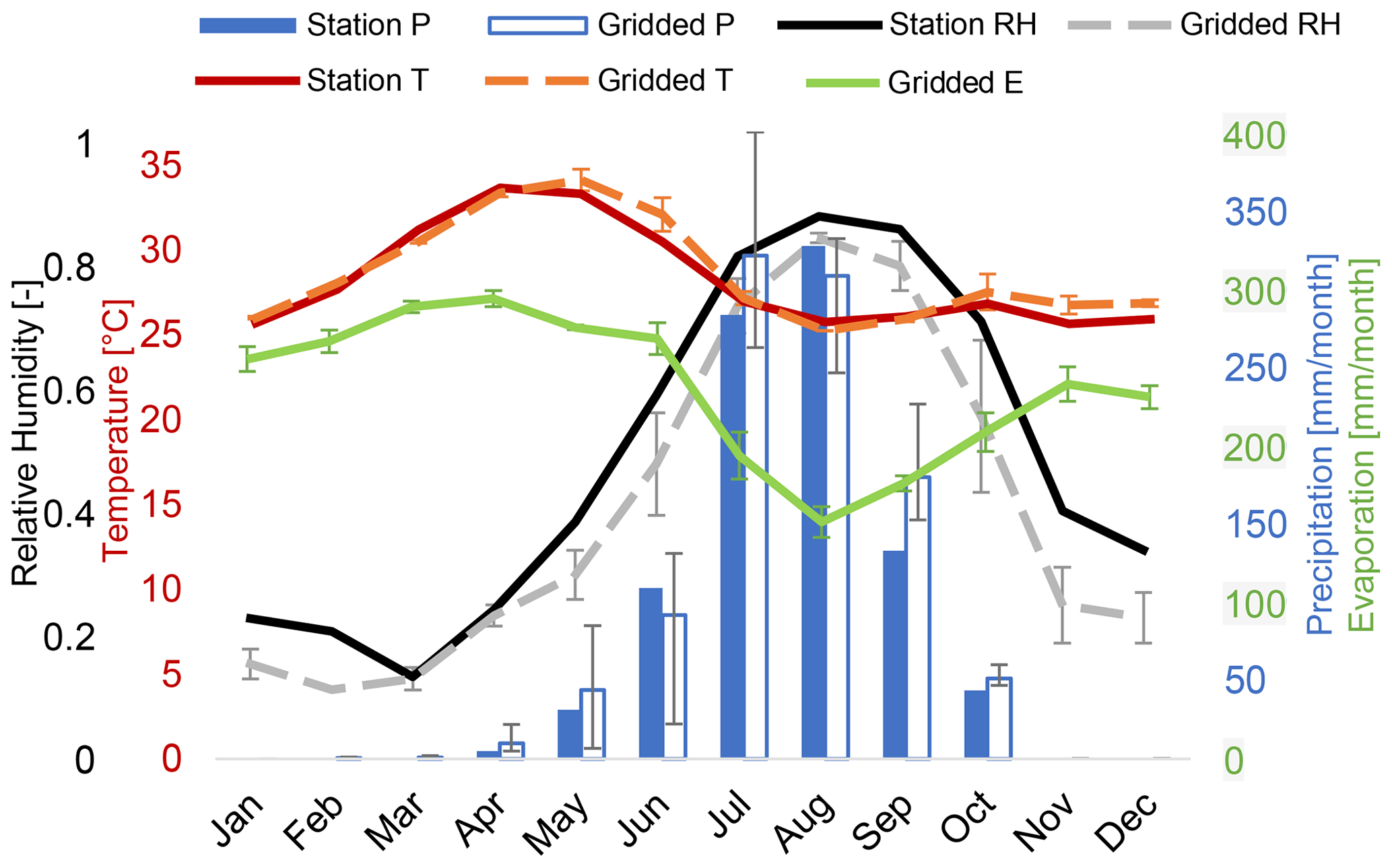
Figure 2 Climate diagram for Guioyo (located 25 km northwest of Lac Wégnia) with data from the period March 2020–February 2021. “Station” refers to the TAHMO station data and “Gridded” refers to the ensemble mean of the gridded global datasets (Table 1). The error bars represent the full range of values among gridded datasets.

4.3 Precipitation

We use the gridded rainfall products (Table 1) to estimate precipitation at Lac Wégnia and the TAHMO station data of 2020 for validation. It can be expected that the different gridded products have a substantially different performance in representing the spatiotemporal rainfall patterns (Dembélé et al., 2020). Here, we only assess the water balance of the dry period, for which rainfall is scarce, and the different products generally agree well with each other (Fig. 2). We therefore use the daily ensemble mean of all eight available products as an input for the precipitation component of the water balance.

4.4 Water surface heights (WSHs)

WSH identification is developed below and implemented as a fully automated processing chain in GEE. The procedure involves the following main steps: (i) remote sensing image selection and pre-processing, (ii) water surface detection, (iii) shoreline detection, and (iv) surface elevation retrieval.

4.4.1 Remote sensing image pre-processing

All satellite images with a cloud percentage over the study area greater than 30 % are excluded from the analysis. The remaining satellite images are co-registered with the orthoimage of the UAV survey in a stepwise manner. First, we select an S2 image that was taken approximately on the same day as the UAV survey (11 May 2019). This image is co-registered with the orthoimage. We then assume that the misalignment of images within the set of images from the same sensor is negligible (Storey et al., 2016; Nguyen et al., 2020) and apply the same displacement to all S2 images. For the Landsat sensors no images are available from the date of the UAV survey. L7 and L8 images are thus co-registered with already aligned S2 images on the same day (25 April 2020 and 11 November 2020, respectively). The L5 and S2 mission periods do not overlap. In a final step L5 images are thus co-registered with a L7 image (9 June 2007).

4.4.2 Water surface detection

Water absorbs most radiation at near-infrared wavelengths and beyond. As a result, water can be easily detected by using spectral indices. Here we use the modification of the normalized difference water index (MNDWI) for land–water classification (Xu, 2006):

$$\begin{array}{}\text{(2)}& \mathrm{MNDWI}=\left(\mathrm{green}-\mathrm{MIR}\right)/\left(\mathrm{green}+\mathrm{MIR}\right),\end{array}$$

where MIR is reflectance in the middle infrared band, and “green” is reflectance in the green band. The MNDWI has been extensively applied for water mapping (e.g., Donchyts et al., 2016; Tseng et al., 2016; Ma et al., 2019), and its good performance has been shown for both Landsat and Sentinel-2 images (Kwang et al., 2017; Yang et al., 2020).

We use a nonparametric unsupervised method based on the Canny edge filter and Otsu thresholding to distinguish between water and non-water pixels, following Donchyts et al. (2016). The Otsu algorithm (Otsu, 1979) is a widely used dynamic threshold method (e.g., Ma et al., 2019; Asfaw et al., 2020; Yang et al., 2020). The method identifies an optimal threshold to distinguish two image classes by maximizing the inter-class variance computed from a normalized image histogram. This requires a bimodal histogram distribution. If land dominates the image over water, the histograms are unbalanced. The Canny edge filter is thus used to reduce the sampling region to only areas near water–land edges. The Canny method first uses a Gaussian filter to smooth the image in order to remove the noise and then finds edges by looking for local maxima of the image intensity gradients. We use the Canny edge algorithm with the following parameters to process all images: σ=0.7 (standard deviation of the Gaussian smoothing kernel), th=0.7 (threshold used to define the sensitivity of the gradient magnitude filter), an image pixel resolution of 30 m, and a buffer around the edges of 60 m.

Binary water images are obtained at the native resolution of the sensors (30 m for Landsat, 10 m for Sentinel-2). The area of Lac Wégnia can be obtained from these images after gap filling. A simple focal-mode filter is applied to fill data gaps and void stripes in Landsat 7 images. Note that gap filling is not required for WSH retrieval, which is another advantage of the method over AV scaling.

4.4.3 Shoreline detection and elevation retrieval

The shoreline is defined as the water–land boundary of the binary water image. To retrieve the elevation of the shoreline, a 10 m buffer is added on both sides of the edge. Within this buffer we sample all DEM pixel values at a 10 m resolution and use the median to calculate a single WSH. Weekley and Li (2019) obtained slightly better results using the mean instead of the median. However, the median is less sensitive to noise and shoreline elevation anomalies (see Sect. 4.5).

A variety of factors such as local slope, mixed pixels, and water detection accuracy can impact the accuracy of the retrieved WSH (Tseng et al., 2016; Weekley and Li, 2019). Because surface water may not be correctly identified under canopies, we mask all boundary pixels that are adjacent to lush vegetation (NDVI >0.5). Note that at Lac Wégnia this situation only occurs during the wet season when the lake is completely filled. Pixels for which the retrieved mean erosion–deposition rate exceeds 10 mm yr⁻¹ are also removed from calculating the final WSH (see Sect. 4.5 below). Unfortunately, no in situ water level data are available for Lac Wégnia for a validation of the retrieved WSH data. We therefore only assess the relative accuracy of the approach by comparing WSH data obtained for the same or subsequent days from different images (acquired by Landsat and Sentinel-2 satellites).

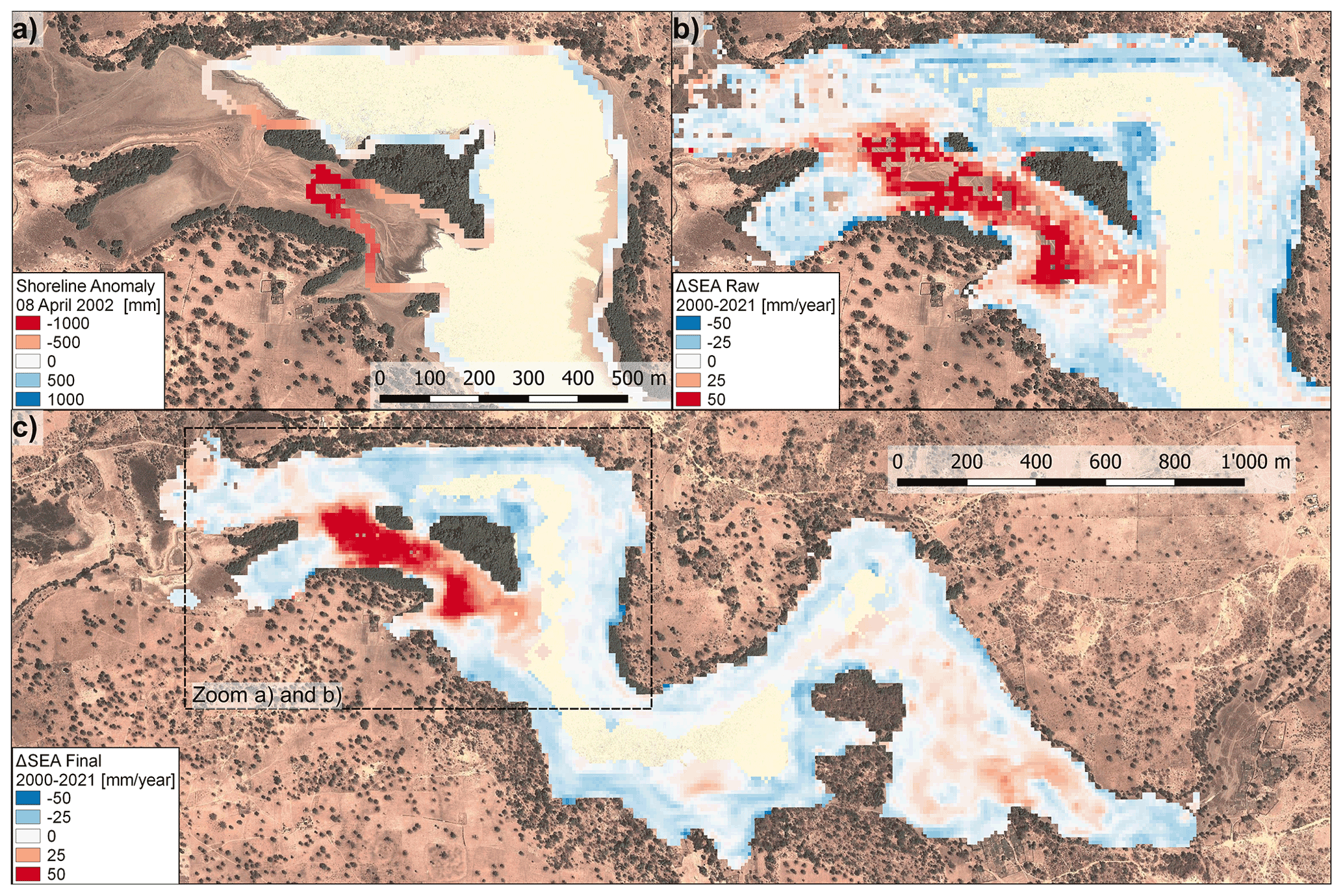
Figure 3 (a) Shoreline elevation anomalies of a Landsat 7 scene from 8 April 2002. (b) Slope of shoreline elevation anomalies (ΔSEA) for 2000–2021 in meters per year. Shown are all 10 m pixels for which data points are available from at least 6 years. (c) Gap-filled and outlier-corrected map of ΔSEA 2000–2021. Red and blue pixels point to sediment deposition and erosion, respectively. This map is used to calculate the sediment balance of Lac Wégnia. The background image is a Google Earth image from 23 March 2013 (© Google Earth 2021).

4.5 Sediment balance

The waterline method is based on the assumption of common heights of geocoded waterline pixels (Salameh et al., 2019). However, this assumption is only valid if either the elevation information is available exactly for the time of the lake boundary acquisition or if the bathymetry of the lake does not change over time. In our case a DEM is only available for May 2019, and it is very likely that over the study period of 1999–2021 there are changes in the lakeshore and bed topography due to sediment deposition and erosion. Deposition occurs preferentially on sediment deposit cones, while lakeshore erosion may take place where the banks are not protected by littoral vegetation and where rills and gullies are formed. Such local topographic changes become visible by comparing the waterlines of two scenes which represent approximately the same water level. At sediment deposition cones the waterline of the older scene bends much more inland than the more recent scene (Fig. 3a) and vice versa at erosion zones. If such “shoreline anomalies” are not too numerous, the median of all shoreline pixel elevations still provides a valid estimate of the water surface elevation, even if the lake boundary of an older scene is projected on the recent lake bathymetry. The difference between the median elevation of all shoreline pixels and a pixel elevation at a shoreline anomaly is then equal to the elevation change that has occurred at that point. In the following, we call these deviations from the median “shoreline elevation anomalies” (SEAs).

$$\begin{array}{}\text{(3)}& {\mathrm{SEA}}_{i,t}={\mathrm{WSH}}_t-{\mathrm{SE}}_{i,t}\end{array}$$

SEA_i,t in Eq. (3) is the SEA at time t at pixel i, SE_i,t is the shoreline elevation at pixel i according to the current bathymetry, and WSH_t is the median of all shoreline pixel elevations. If an SEA is positive, then erosion has since occurred, and if it is negative, deposition has occurred.

SEAs also occur if the scenes providing the lake boundaries are not well aligned with the DEM or if the shoreline delineation is erroneous. For this reason it is important to look at the evolution of SEAs over time to get a robust picture of the nature of geomorphic change on the lake shoreline. SEAs should continuously change over time at deposition or erosion zones. While SEA values for individual dates may represent noise, the longer-term trend in SEA values (ΔSEA, units mm yr⁻¹) points to deposition and erosion processes. Robustly increasing or decreasing SEA slopes can then be assumed to be equivalent to sediment deposition or erosion rates, respectively. Furthermore, SEAs may occur because of topographic slopes within the ±10 m buffer that is used for sampling shoreline pixels. For this reason, SEAs extracted at 10 m pixel resolution are smoothed by applying a morphological mean filter within 30 m square kernels.

The complete procedure to extract maps of ΔSEA can be summarized as follows. (1) Identifying the WSH of a given scene as described in Section 4.4.3. (2) Mapping of SEAs within the ±10 m buffer of each lake boundary. (3) Smoothing of SEAs with the morphological mean filter. (4) Taking the mean of all SEAs over a given pixel for a given hydrological year, resulting in 22 annual SEA maps (hydrological years 2000–2021). (5) Applying a nonparametric Sen's slope estimator to calculate ΔSEA. Sen's slope is less sensitive to outliers than the common least squares estimate using linear regression (Sen, 1968).

The validity of the procedure depends on the assumption that the median shoreline pixel elevation is a robust estimator of actual WSH. To test this assumption, steps 1–5 above are applied iteratively by always masking out areas where absolute ΔSEA exceeds 10 mm yr⁻¹ in step 1. Therefore, locations where anomalies occur get excluded from calculating WSH. After each iteration the average ΔSEA within the lake bed is calculated (hereafter referred to as the “sediment balance”), as is the fraction of the area where absolute ΔSEA does not exceed 10 mm yr⁻¹. If both indicators converge to stable values after 10 iterations, the resulting ΔSEA map can be used to identify the deposition and erosion areas that need to be masked for the calculations of the final WSH values.

Because Lac Wégnia is not an ephemeral lake but shrinks to a small size each dry season, ΔSEA cannot be calculated for lake bed pixels which are rarely or never dry. We apply a minimum threshold of six annual SEA values (∼30 %) that need to be available in order to calculate ΔSEA. Data gaps in the map (Fig. 3b) are filled with a focal mean filter (Fig. 3c) if pixels with ΔSEA values are present within a two-pixel (20 m) radius.

4.6 Trend analysis

We look for trends in the seasonal mean values of each water balance component (Eq. 1). Regression slopes are estimated using the method of Theil (1950) and Sen (1968), hereafter called Sen's slopes, and uncertainty ranges are provided by the 95 % CI of the Sen slope estimate computed using the Gilbert (1987) modification of the Theil–Sen method. The significance of the trend is assessed by Kendall's nonparametric test for a monotonic trend (Kendall, 1975).

To explain the observed lake level trends we perform an attribution analysis. Three main factors determine the lake level at the end of the dry season: (i) the initial lake level, (ii) the mean rate at which the lake level decreases over the dry season, and (iii) the length of the dry season. Changes in these three independent factors over the last 22 years can explain the observed lake level trends:

$$\begin{array}{}\text{(4)}& \mathrm{\Delta }{h}_{\mathrm{tot}}=\mathrm{\Delta }{h}_{\mathrm{rate}}+\mathrm{\Delta }{h}_{\mathrm{ini}}+\mathrm{\Delta }{h}_{\mathrm{\Delta }t}\approx \mathrm{\Delta }{h}_{\mathrm{obs}},\end{array}$$

where Δh_rate represents the lake level change that is due to the change in the rate at which the lake level decreases over the dry season, Δh_ini is the change in initial lake levels, and Δh_Δt represents the lake level change due to changes in the timing of the wet season. The sum of all effects (Δh_tot) should be approximately equal to the observed difference in dry-season lake levels (Δh_obs). Each factor is quantified based on the available WSH time series as explained in Sects. 4.6.1–4.6.3 below.

4.6.1 Dry-season lake level change rates

The number of available WSH data points varies between years due to clouds and dust storms and due to the different mission periods of the satellites. To enable comparison of WSH change rates it is therefore necessary to homogenize the WSH time series. For each hydrological year, the available data are extrapolated to cover the full dry-season period from 1 October to 15 May. The steps for extrapolation of the data are the following. (1) Smoothing the WSH time series with a 7 d window running-mean filter. (2) Calculation of the WSH change rate (Δh, units mm d⁻¹) between all subsequent dry-season data points that are separated by 8–16 d (16 d is the usual Landsat overpass interval). (3) The day of the year (DOY) of the last day of each interval is attributed to each available data point. The cloud of points is converted into a time series of average Δh seasonality by smoothing again with a 7 d window running-mean filter. (4) Data gaps are filled by using the average Δh seasonality as follows:

$$\begin{array}{}\text{(5)}& \mathrm{\Delta }{h}_{\mathrm{gap}}=\sum _{i=t_{\mathrm{1}}}^{t_{\mathrm{2}}}\mathrm{\Delta }{h}_{{\mathrm{ref}}_i}\times {\displaystyle \frac{\mathrm{\Delta }{h}_{{\mathrm{obs}}_{t\mathrm{3}-t\mathrm{4}}}}{{\sum }_{i=t_{\mathrm{3}}}^{t_{\mathrm{4}}}\mathrm{\Delta }{h}_{{\mathrm{ref}}_i}}},\end{array}$$

where Δh_gap is the interpolated WSH change (units mm) for a given time period of missing data between t₁ and t₂, $\mathrm{\Delta }{h}_{{\mathrm{ref}}_i}$ is the reference WSH change (units mm d⁻¹) described by the average Δh seasonality for a given DOY, and $\mathrm{\Delta }{h}_{{\mathrm{obs}}_{t\mathrm{3}-t\mathrm{4}}}$ is the observed WSH difference between t₃ and t₄. The time period t₃ to t₄ has to cover at least 50 % of the entire period of 1 October to 15 May. Hydrological years for which less than 50 % of the dry period is covered by available WSH observations are not considered for the Δh_rate trend analysis. For all other hydrological years, an average Δh_rate is calculated based on the gap-filled dry-season WSH difference. The Sen slope test is applied to assess the multiyear trend in Δh_rate. The gap-filled dry-season WSH difference is also used together with E and P to derive ΔQ for each hydrological year based on Eq. (1).

4.6.2 Initial lake levels

During the wet season when the lake is completely full, the lake level raises above the elevation of the outlet and consequently the outflow becomes activated. However, shortly after the end of the wet season, due to the lack of further inflow into the lake, the lake level equals the elevation of the outlet (hereafter also called the “dead storage level”) and runoff from the lake dries up. This dead storage level can be seen as the initial water level at the beginning of each dry season. The dead storage level may change over time because of geomorphological changes in the natural levee at the lake outlet but at scales that are too fine to resolve with our sediment balance approach. No direct measurements of the dead storage level are available except for 2019 when the minimum elevation of the outflow channel was 329.8 m a.s.l. As a proxy for past dead storage levels we thus determine the initial dry-season lake levels of each hydrological year. The 1 October WSHs of the homogenized WSH time series (see Sect. 4.6.1) are used for this purpose. The Sen slope test is then applied to assess the changes in initial lake levels (Δh_ini).

4.6.3 Timing of the wet season

To determine the beginning and the end of the wet season we calculate weekly totals of open-water evaporation and compare them with the precipitation sum of each calendar week. The beginning of the wet season is then defined as the first week in the year when the weekly precipitation sum exceeds the weekly evaporation. Accordingly, the dry season starts the week after the last week in the year when weekly P exceeds weekly ET. Changes in the DOY of the dry-season onset are assessed by applying the Sen slope test. To translate these changes into millimeters of water (Δh_Δt), the Sen estimate of the slope is multiplied by the multi-annual mean daily lake level change calculated based on the average Δh seasonality (see Sect. 4.6.1).

If the lake level decreases below 328.64 m a.s.l. the lake level cannot be determined because the bathymetry below that level is unknown. For some years we therefore have data gaps in the WSH time series in late May and June. For this reason, the effect of changes in the timing of the onset of the wet season on water levels is not assessed quantitatively. Because such data gaps rarely occur before 15 May, only WSH data points until that day are considered for assessing the change in end-of-dry-season lake levels.

5 Results

5.1 Validation of gridded datasets

The following variables from the gridded datasets can be validated against station data from Guioyo: precipitation, air temperature, and relative humidity (Fig. 2). Precipitation and relative humidity reveal strong seasonality with a peak around August. From November to April precipitation is practically zero. Temperature is relatively constant throughout most of the year (July to January), with slightly higher values towards the end of the dry season (April–May). The gridded datasets reproduce this seasonality very well (Fig. 2). Also, in terms of absolute differences the gridded datasets agree well with the station data: the mean monthly absolute difference between the ensemble of gridded datasets and the measurements is only 0.6 ^∘C (temperature), 12 mm (precipitation), and 8 % (relative humidity).

5.2 Lake water areas

In total, 541 satellite images from 527 d within the period 1 October 1999 to 30 June 2021 fulfill the quality criteria and are available to extract WSH data (Fig. 4a). The number of available scenes per year increases strongly in the year 2013 when Landsat 8 was launched and again in 2016 when Sentinel-2 data became available. The minimum number of scenes available per year is 4 (years 2001 and 2004), whereas the maximum is 70 (year 2020).

The extracted lake areas reveal strong seasonality in lake extent, ranging between 1 and 157 ha (Fig. 4a). The lake never fell entirely dry in the study period (de La Rocque and Renoullin, 2015).

81.9 % of the 10 m pixels within the maximum lake extent area represented the shoreline in at least one scene over the entire study period. For 5.8 % of the area no data are available because of data gaps in the DEM. The remaining 12.3 % of the area either never represented the shoreline or was masked from the DEM because of adjoining canopies below which the shoreline could not be seen.

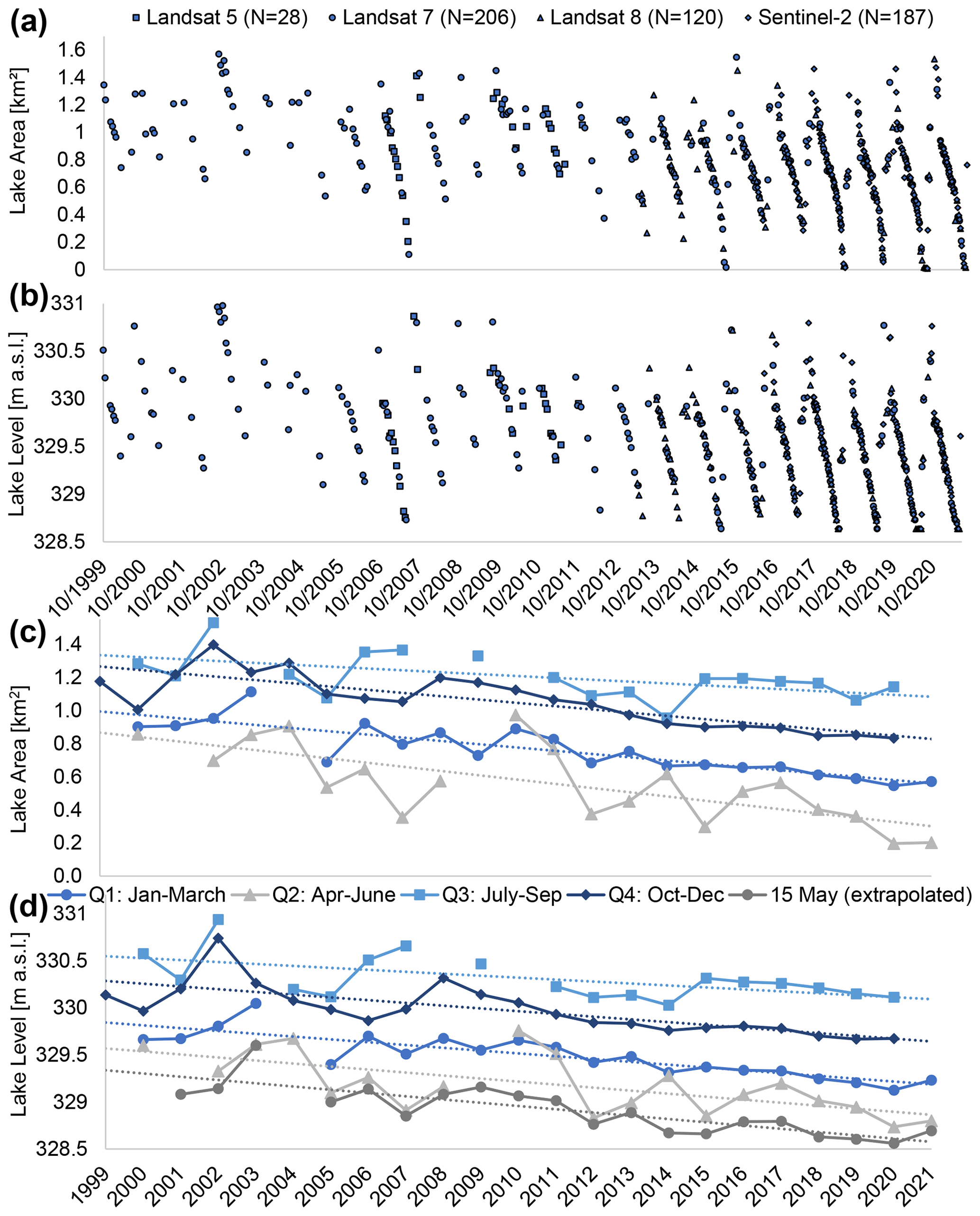
Figure 4 Time series of (a) lake area and (b) lake water level retrieved from Landsat 5, 7, and 8 as well as Sentinel-2 optical satellite imagery for the period 1 October 1999 until 30 June 2021. N is the number of scenes available from each sensor. In total 541 scenes are represented. (c) Annual average quarterly lake areas and (b) lake levels with associated linear trend lines. Lake levels from 15 May in (d) represent the level at the approximate end of the dry season and are identified based on extrapolated lake levels (Fig. 10).

5.3 Sediment deposition and erosion areas

The iterative approach to identify shoreline elevation anomalies converged to stable solutions after about five iterations (Fig. 5). After 10 iterations, the fraction of the area where absolute ΔSEA does not exceed 10 mm yr⁻¹ converged to about 67 %. This means that 33 % of the pixels for which ΔSEA estimates are available represent deposition or erosion areas that needed to be masked for obtaining the final WSHs. The sediment balance for 2000–2021 of the lake bed below the dead storage level in May 2019 converged to a value of −44 mm (Fig. 5). The negative sign means that there is more erosion than deposition in the lake bed. The sediment balance could also be determined for some areas that are presently located above the dead storage level because they were at a lower level in the past or because they represented the shoreline during the wet season when the lake outflow was activated. Here, the sediment balance was +44 mm, meaning there is more deposition than erosion. Overall, the average of all pixels for which the point sediment balance could be determined is −12 mm in 21 years.

Areas where we observe erosion are distributed over a larger area (20 % of all pixels with a valid result) than the areas where we observe deposition (13 %). The average net sediment deposition rate at locations with more deposition than erosion is 28 mm yr⁻¹, whereas at locations with net erosion the average rate is −16 mm yr⁻¹. Net sediment deposition is concentrated at a few locations such as the river deltas of the southern and eastern tributaries (Fig. 3c). The highest average deposition rates are identified at the western shore of the lake, where the southern tributary flows into the lake (up to +62 mm yr⁻¹). The erosion areas, on the other hand, are stretched along nearly the entire lakeshore (Fig. 3c), whereas the average erosion rates per pixel never exceed −20 mm yr⁻¹.

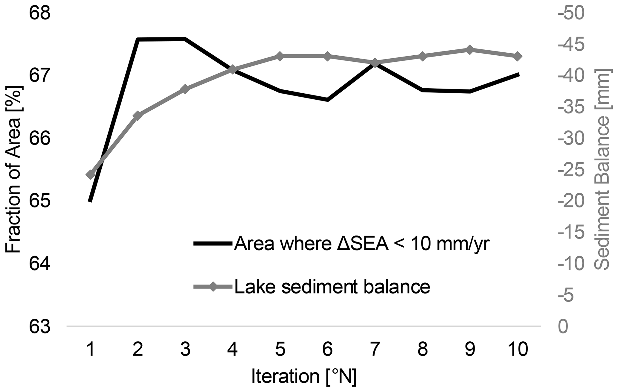
Figure 5 Lake sediment balance for the period 2000–2021 (average ΔSEA within the lake bed) and the fraction of the area where absolute ΔSEA does not exceed 10 mm yr⁻¹ as a function of the iteration number.

5.4 Lake water surface heights

The maximum WSH of the entire study period is 330.98 m a.s.l., reached on 17 October 2002. Assuming that the minimum level was not much below the minimum detectable WSH of 328.64 m a.s.l., the lake levels vary within a range of not more than 2.5 m (Fig. 4b).

The annual average quarterly lake levels reveal negative trends across all seasons (Fig. 4d). All trends are significant at the 0.01 level except the Q3 trend (July–September; $p-\mathrm{value}=\mathrm{0.028}$). The Sen slope of the linear trend lines indicates an average WSH decrease between −0.46 m (Q3) and −0.71 m (Q2: April–June) over the 22-year study period.

20 out of the 541 scenes represent a lake extent that was equal to or smaller than that on 9–10 May 2019. Such data points representing a lake level below 328.64 m a.s.l. still needed to be considered for the calculation of quarterly average lake levels. For the sake of simplicity a WSH of 328.64 m a.s.l. was assigned to such scenes.

More than one satellite image is available for 14 d, and from another 43 d satellite imagery is available from the subsequent day. Excluding 2 d for which the exact water level could not be determined because of the holes in the DEM, we obtain a total of 55 pairs of scenes suitable for analyzing the WSH error. Overall, the absolute WSH errors vary between 0.2 and 161 mm. The median absolute WSH error between scenes from the same day (Δt=0 d, N=13) is 25, and it is 33 mm if the scenes are from subsequent days ($\mathrm{\Delta }t=\mathrm{1},N=\mathrm{42}$; Fig. 6a). If the slope at the waterline was less than or equal to 1^∘, the median absolute WSH error is only 15 mm ($\mathrm{\Delta }t\le \mathrm{1},N=\mathrm{17}$), and it is 51 mm if the slope was above 1^∘ ($\mathrm{\Delta }t\le \mathrm{1},N=\mathrm{38}$).

Figure 6 Analysis of the relative error between water surface heights (WSHs) extracted from Landsat 7 and 8 scenes as well as Sentinel-2 scenes. (a) Box plot of the absolute WSH error between scenes of the same (Δt=0 d) and of subsequent days (Δt=1 d). N is the number of scene pairs available for comparison. The central mark of each box is the median, the edges are the 25th and 75th percentiles, and the whiskers extend to the most extreme data points. (b) Average slopes of waterline pixels and absolute WSH error between scenes of the same or subsequent days (Δt≤1 d).

5.5 Water balance components

Of the four water balance components, evaporation rates (E) and daily WSH changes (Δh_rate) show the most pronounced seasonality over the course of the dry season (Fig. 7). Daily rates of E increase from about 7 mm d⁻¹ in October to about 10 mm d⁻¹ in April. Δh_rate shows a similar behavior, but the rates are about 2 mm d⁻¹ lower than the daily rates of E. Because P is usually zero during the dry season, the difference between E and Δh_rate is made up by net inflow (Q). Net inflow is positive, which means that inflow is higher than outflow. Only at the beginning of the dry season, in October, is the outflow from the lake possibly still higher than inflow (Q<0 mm d⁻¹), but the uncertainty in the calculated rates is high (Fig. 7).

The average seasonality of Δh_rate that is described above is used to fill data gaps in the WSH time series, therefore enabling us to calculate average rates for the dry season of each hydrological year 2000 to 2021 (Fig. 8). Only in two years (2000 and 2004) do the available observations cover less than 50 % of the dry season, and WSHs of these years were therefore not extrapolated. The Sen slopes of the remaining 19 annual values indicate a positive trend in daily rates of E and Δh_rate, a negative trend in Q, and no trend in P (Fig. 8).

Figure 7 Rates of water balance components (lake level change: Δh_rate, net inflow: Q, precipitation: P, evaporation: E) during the dry season (1 October until 15 May). The lines and error bars indicate the mean and standard deviation, respectively, over available data points for 15 d periods. For precipitation the median and the 95 % confidence interval are shown instead of the mean and the standard deviation.

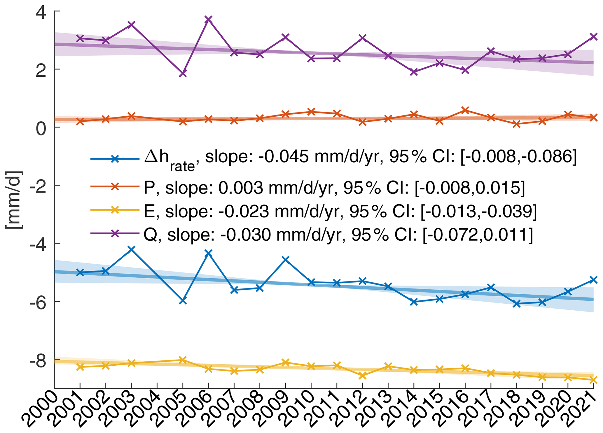
Figure 8 Average daily rates of water balance components estimated for the dry seasons in 2000–2021 (lake level change: Δh_rate, net inflow: Q, precipitation: P, evaporation: E). The transparent areas show the 95 % CI of the linear regression slope.

5.6 Attribution analysis

The accelerating dry-season WSH decrease leads to lower lake levels at the end of the dry season. The observed trends in Δh_rate cause a decrease in end-of-dry-season lake levels between 37 and 406 mm over the 22-year period (Fig. 9), considering the 95 % confidence interval (CI) of the Sen slope of the linear regression (Fig. 8). The accelerating lake level decrease can be explained by the increase in direct evaporation from the lake, explaining 62 to 186 mm of the observed negative trend in lake levels. Likely, a decrease in net inflow also contributed to a decrease in WSHs. However, according to the test for a monotonic trend, there is a probability of 14 % that net inflow has increased rather than decreased. The 95 % CI ranges from an impact on the lake level between +50 and −338 mm that is due to changes in net inflow (Fig. 9).

The observed lake level decrease over the 22-year period is much higher than what can be explained by the changes in dry-season water balance components. The average lake levels of the months January–March decreased by 644 mm (Figs. 4c and 9, 95 % CI: 451–865 mm). The extrapolated lake levels for 15 May (Fig. 10a) decreased by 414–845 mm (Fig. 4c). Even the average lake levels of the wet season decreased by 458 mm (Q3 in Fig. 4c), but the uncertainty of the regression is high (95 % CI: 33–853 mm). Variations in the timing of the dry season also cannot explain the observed lake level trends (Fig. 11).The test for a monotonic trend does not indicate that an earlier or later end of the wet season has a significant impact on the multiyear trend in WSH (Δh_Δt in Fig. 9).

In spite of an increasing trend in wet-season precipitation (ensemble mean of all precipitation products; see Table 1), the initial lake levels at the beginning of the dry season have been decreasing over time (Fig. 10). The decreasing initial lake levels explain 260–647 mm of the observed overall dry-season lake level decrease (95 % CI, Δh_ini in Fig. 9).

The sum of the Sen slope for Δh_ini, Δh_rate, and Δh_Δt results in a reconstructed lake level decrease of 631 mm (95 % CI: 377–958 mm, Δh_tot in Fig. 9), which is very similar to the measured lake level decrease (644±207 mm, Δh_meas in Fig. 9). Changes in Δh_rate explain about 34±18 % of the decrease, Δh_Δt explains 0±11 %, and the changes in initial lake levels explain the largest portion of the reconstructed dry-season lake level changes (66±18 %).

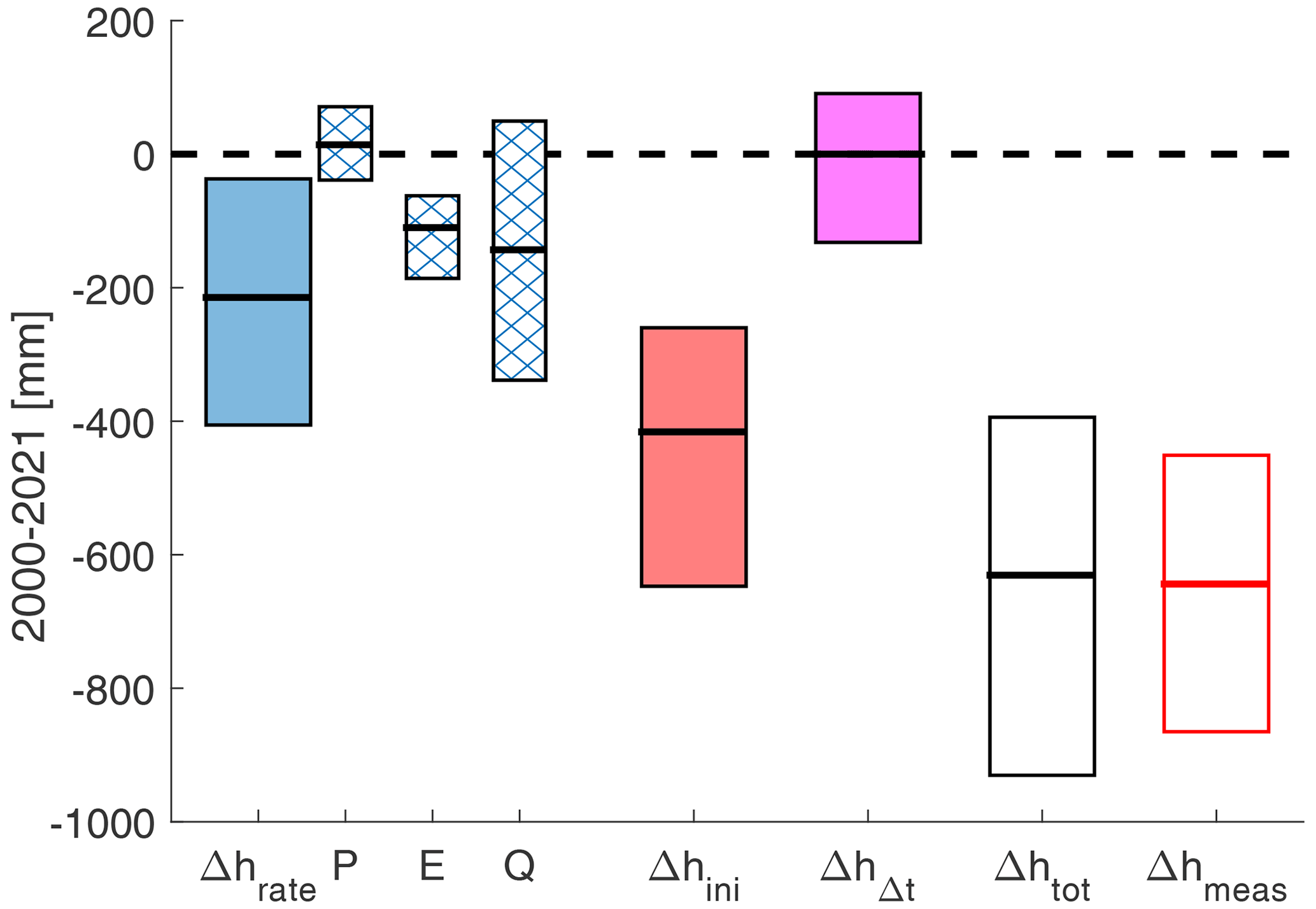
Figure 9 Impacts of hydrological changes on end-of-dry-season lake levels (95 % CI). Δh_rate represents the increasing rate of WSH decline during the dry season that is due to changes in precipitation (P), open-water evaporation (E), and net inflow (Q). Δh_ini represents the impact of lower initial lake levels at the beginning of the dry season, and Δh_Δt represents the lake level change due to changes in the timing of the wet season. Δh_tot is the sum of Δh_rate, Δh_ini, and Δh_Δt. Δh_meas is the measured difference in dry-season lake levels between 2000 and 2021 (Q1 in Fig. 4).

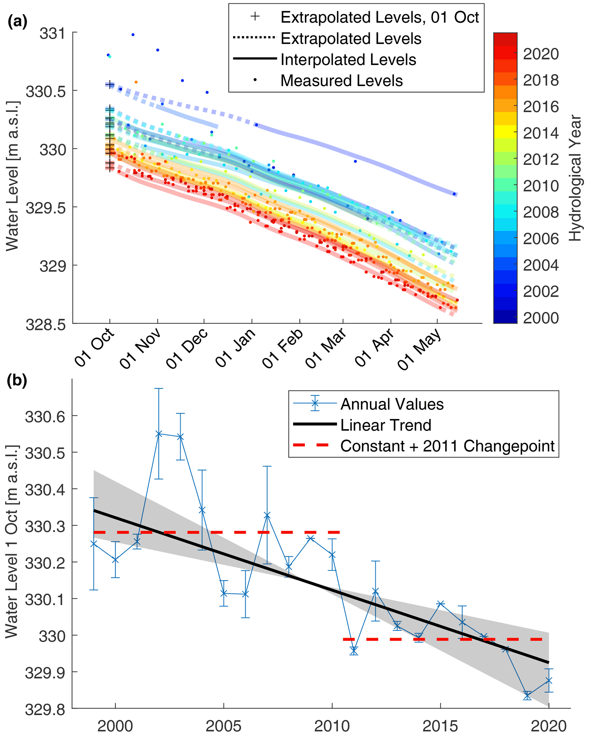
Figure 10 (a) Dry-season water levels for each hydrological year from 2000–2021. The crosses indicate the extrapolated WSH on 1 October, which is used as a proxy for the floor level at the outflow. Values above 330.4 m a.s.l. are considered outliers and are not considered for extrapolation. (b) Time series of extrapolated WSH on 1 October. Error bars represent the range of values obtained by considering the uncertainty in the rates used for extrapolation (Fig. 7). The transparent area indicates the 95 % CI of the linear regression slope. The dotted red line shows an alternative interpretation of the data, speculating that a single strong erosive event in 2011 may have lowered the outflow level by approximately 29 cm.

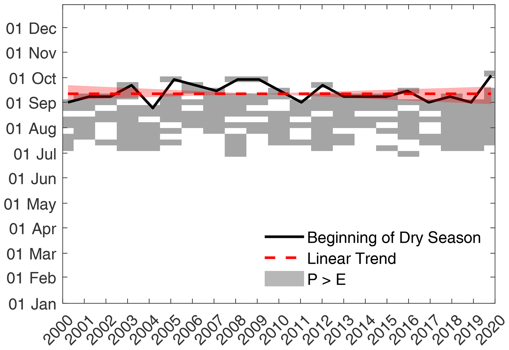
Figure 11 Date of the beginning of the dry season based on gauge-corrected satellite data (black line). The dry season is defined as the portion of the year when open-water evaporation (E) exceeds precipitation. Weeks with sufficient precipitation to satisfy E are marked in grey. The dotted red line indicates the linear regression line based on the Sen slope estimator.

6 Discussion

The careful separation of the lake sediment and the lake water balance allows us to unambiguously attribute causes to the observed trend of an ever more diminishing lake surface (Fig. 4c). The average over all grid points is negative ($-\mathrm{43}\pm \mathrm{1}$ mm over the period 2000–2021), which means that there is more erosion than deposition, and therefore silting is not the cause of the observed lake area decrease (minus 22–54 ha across all seasons, see Fig. 4c). Still, as expected, net sediment deposition is evident at the depositional plains downstream of the two tributaries. With the derived sedimentation and erosion rates for each pixel we can reconstruct the bathymetry of Lac Wégnia from the beginning of the century and compare the lake areas for given WSHs. If the WSH is between 329.4 and 329.9 m a.s.l., the lake area today is up to 4.5 ha smaller than 21 years ago (Fig. 12a), which represents about 5 % area loss.

At an elevation range between 328.7 and 329.3 m a.s.l. the lake has seen a net erosion of the lake bed (Fig. 12). According to the sediment balance, about 40 000 m³ of soil eroded from this zone over the last 21 years. The areas which see a net erosion of the ground are characterized by gentle slopes and are frequently visited by livestock for watering. The bare silty soil dries out during the dry season, gets mobilized by the cattle, and then gets suspended in the water when the water is rising again. Our calculations cannot clarify if the sediments are moved from there to deeper areas of the lake where they deposit again or if they get flushed away during the wet season. Given the fine grain size of the material we suspect that the latter is the case.

The attribution analysis has revealed that the main cause of the decreasing dry-season water level trend is lower initial lake levels at the beginning of the dry season (Fig. 9). The initial lake levels are crucial for the persistence of the lake during the dry season because the lake does not see any surface water inflow over a period of about 8 months. Less than 30 % of the water that evaporates is replaced by net inflow through groundwater exchange (Fig. 8). Decreasing initial lake levels therefore imperatively lead to decreasing WSHs at the end of the dry season. The lake might even run completely dry in the future, which is something that has never occurred in the past decades.

The lake levels at the end of the wet season mainly depend on the base level at the outflow, which defines the dead storage volume of the lake. The sediment balance around the location of the outlet indicates net erosion rates of 10±13 mm yr⁻¹, which is less than the 20±3 mm yr⁻¹ obtained for Δh_ini (Fig. 9). However, the outflow channel is only about 5 m wide and is therefore below the pixel resolution of the sediment balance map (Fig. 3c). A handmade dam with a height of about 50 cm made out of sand bags was present at the location during field visits in 2019 and 2020 (Fig. 13). According to information from local residents, the dam is not able to withstand the speed of the water leaving the lake during the rainy season and thus collapses, but it has been rebuilt each year since 2009 to reduce the outflow of water from the lake. As a consequence of the collapse of the dam, the flow velocities increase, which leads to temporarily higher erosion rates. The step between 2010 and 2011 in the time series of the 1 October water level (Fig. 10b) coincides with the timing of the first construction of the dam. The average reconstructed water levels are 29 cm higher at the beginning of the dry seasons in 1999–2010 than over the period 2011–2020 (Fig. 10b). The intervention in the riverbed in 2009 may thus have entailed a strong erosive event during the wet season of the year 2011.

Of course, lower WSHs at the beginning of the dry season could also be caused by changes in the wet-season water balance. However, the lake exceeded a level of 329.8 m a.s.l. during each wet season of the observation period (Fig. 4b). The lake thus continues to exceed the dead storage level of May 2019, which means that during the wet season, the lake recovers from the low WSHs at the end of the dry season. The duration of the wet season also did not change significantly over the observation period (Fig. 11). Our analysis even reveals positive wet-season precipitation trends for Lac Wégnia (Table 1), confirming recent findings by, e.g., Nouaceur and Murarescu (2020) and Bodian et al. (2020). These findings do not suggest that the observed changes in initial WSH at the beginning of the dry season depend on wet-season water balance changes. On the other hand, a lower dead storage level can explain the tendency of lower WSHs during the wet season (Fig. 4d) because with a lower base level at the outflow, much higher inflows would be required to reach the same water levels. Following this interpretation, according to Fig. 10b, the dead storage level of Lac Wégnia has decreased by 0.3 to 0.6 m. This is equivalent to a storage volume loss of 300 000 to 700 000 m³. About 25 % to 50 % of the storage capacity has therefore been lost since the beginning of the century.

The present study also indicates a possible decrease in net inflow to the lake during the dry season and an increase in direct evaporation from the lake (Fig. 9). Increasing evaporation may be related to increasing air temperature (Touré Halimatou et al., 2017). Since net inflow is predominantly positive (Fig. 7) but there is no surface inflow to the lake during the dry season, the inflow enters the lake through groundwater exchange. This contribution would be reduced by dropping groundwater levels, and the lake levels would gradually decrease. However, the uncertainty range of the calculated net inflow indicates that groundwater levels could also be stable (Fig. 9). Indeed, a general decrease in groundwater levels should also affect the levels and extent of other water bodies in the area, but the surface water areas of Lac Kononi in the vicinity of Lac Wégnia do not show a decreasing trend over the last 22 years (Fig. A1). Lac Kononi is a groundwater-fed lake that is not directly connected to a river channel, and its water level can therefore be used as a proxy for local groundwater levels. Unfortunately, the bathymetry of Lac Kononi is not available, and we therefore could not reconstruct its WSH as we have done for La Wégnia. Its constant lake areas, however, are an indicator for stable groundwater levels. Groundwater is not continuously monitored in the region, and it is therefore not possible to draw a final conclusion. Our findings highlight the need for the monitoring of groundwater in the region, which has an important ecological role and which is an important resource for human activities.

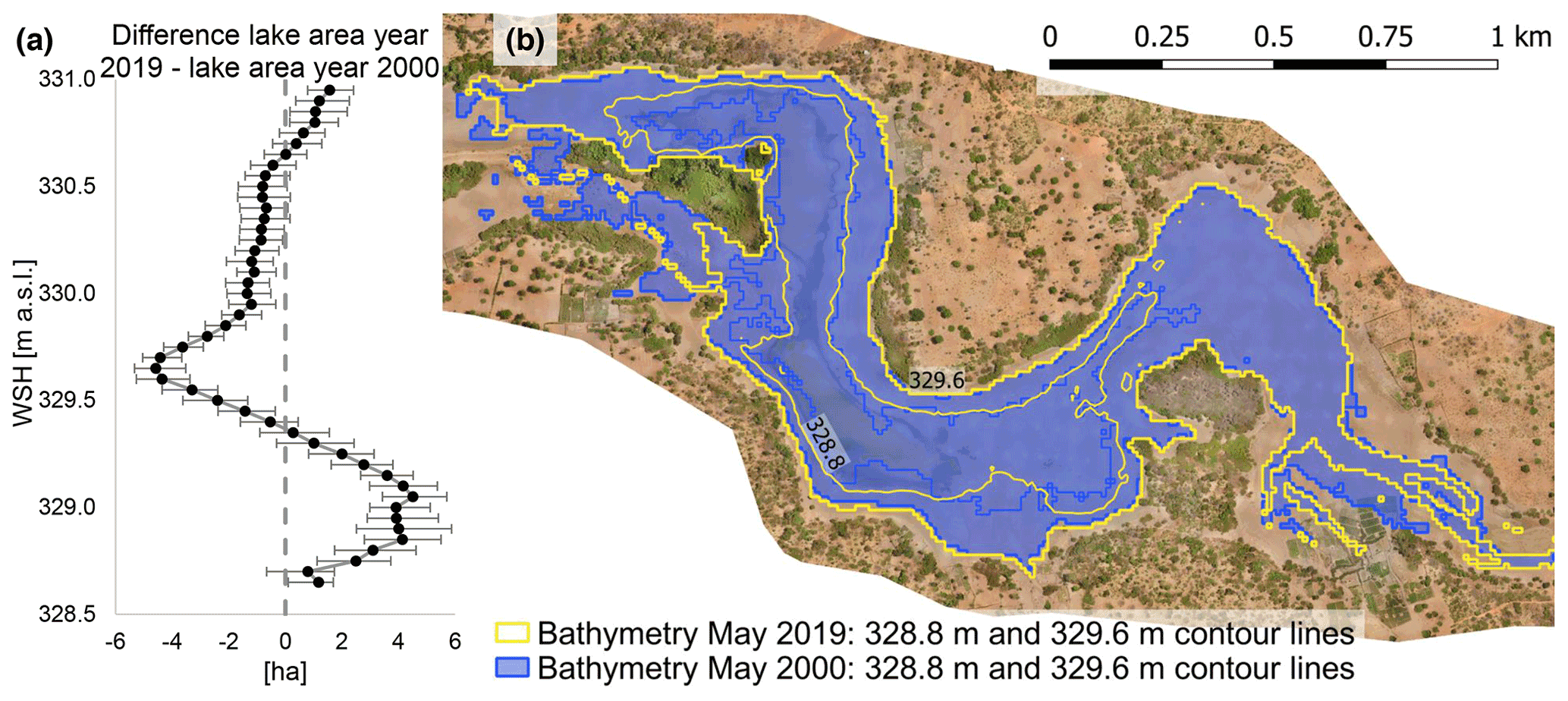
Figure 12 (a) Difference in lake area as a function of water surface height (WSH) based on the bathymetries for May 2019 and May 2000. The error bars reflect the 95 % CI of the sediment erosion and deposition rates that were used to reconstruct the bathymetry of the year 2000. (b) Lake contour lines for a WSH of 328.8 m a.s.l. and 329.6 m a.s.l. considering the bathymetries of the years 2000 and 2019, respectively.

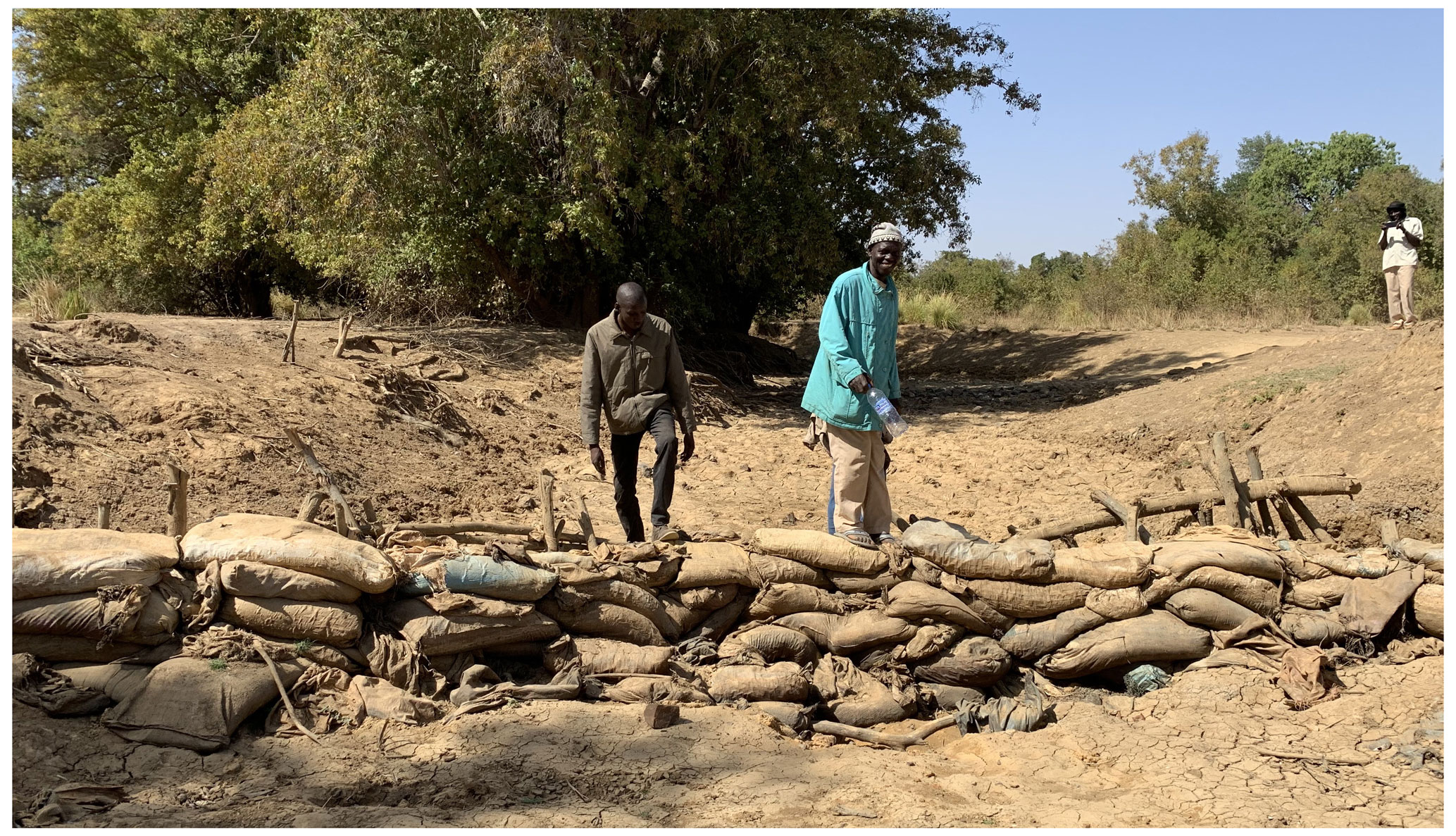
Figure 13 Photo of the handmade dam at the outlet of Lac Wégnia (9 February 2020, source: Tobias Siegfried).

7 Uncertainty assessment

Shallow slopes greatly increase the accuracy of the waterline approach (Tseng et al., 2016). The steeper the slope, the larger the elevation range within a Landsat or Sentinel-2 pixel that represents the lakeshore. The average slope of shoreline pixels at Lac Wégnia is between 0.2 and 2.25^∘ per scene, with an average of 1.06^∘ across all scenes that represent a WSH below outflow level (329.8 m a.s.l.). Assuming a horizontal error of the waterline position of one pixel (i.e., 30 m for Landsat scenes and 10 m for Sentinel-2 scenes) and a slope of 1.06^∘, we obtain vertical errors of 0.56 m (Landsat) and 0.18 m (Sentinel-2). The average number of 10 m shoreline pixels per scene is n=671 (WSH below 329.8 m a.s.l., excluding masked pixels). Assuming that the vertical error estimates above represent the standard deviation (σ) of each pixel-wise WSH estimate, we obtain a standard error of the WSH equal to $\mathit{\sigma }/\sqrt{n}$ and therefore 21 mm (Landsat) and 7 mm (Sentinel-2). These theoretical errors agree well with the identified relative errors (Fig. 6) and demonstrate that the waterline approach provides sufficient accuracy for the purpose of identifying WSHs at Lac Wégnia.

For the shoreline elevation anomalies the same considerations of accuracy apply as for the WSH estimates. The accuracy of the sediment balance estimates then mainly depends on the adequacy of the regression slopes fitted to the SEAs. For individual pixels, the average 1-σ CI of the Sen slope is quite large (±7.8 mm yr⁻¹, resulting in an uncertainty of the pixel-wise sediment balance of ±163 mm over 21 years). Sediment balances of individual pixels should therefore be interpreted with care. However, the total number of pixels for which sediment balances could be calculated is n=10 790, and the standard error of the lake sediment balance is therefore only 1.6 mm. The resulting deposition–erosion patterns (Fig. 3) agree well with the expected patterns (see the section above), which demonstrates the suitability of the approach.

The point sediment balances at individual pixels are sensitive to errors in the co-registration. According to Nguyen et al. (2020), the random offset differences between Landsat 8 and Sentinel-2 can be reduced to less than 2 m in most of the pixels with the displacement() function in GEE. We thus tested the sensitivity of the lake sediment balance to a random error in co-registration by adding a random error with a normal distribution (μ=0, σ=2 m) to the determined displacements (in both the X and Y direction). The resulting lake sediment balance over the 22-year study period changed by +9 mm from −44 to −35 mm, which can be considered an acceptable error range.

The uncertainty assessment above confirms the findings of previous studies (e.g., Tseng et al., 2016) that the accuracy of the waterline method greatly benefits from shallow slopes at the waterline, a sufficiently large number of shoreline pixels, and a low shoreline positioning uncertainty. Furthermore, our analysis benefits from high relative vertical accuracy of the DEM, cloud-free meteorological conditions during the dry season, and strong natural fluctuations of the water level. With the exception of the availability of a high-resolution DEM, the factors named above are valid for hundreds of water bodies in the Sahel and beyond. Assuming similar boundary conditions for other water bodies in the region and an acceptable sediment balance standard error of 10 mm, our approach can also be applied to ponds and reservoirs that are up to 40 times smaller than Lac Wégnia (i.e., average surface water areas of up to 2.5 ha).

Regarding the availability of lake bathymetries, our study has shown that a single UAV survey is sufficient to satisfy this point. However, We recognize that UAV surveys are impractical in many locations due to security concerns and the remoteness of the water bodies in the region. Satellite altimetry can therefore be a promising alternative for data collection in the field. Armon et al. (2020) have shown that determining the bathymetry of shallow desert lakes using ICESat-2 altimetric tracks is possible. For Lac Wégnia, however, ICESat-2 cross-sections are not yet available for the central part of the lake.

8 Conclusions

This work has demonstrated the utility of the waterline method for extracting the water levels of Lac Wégnia, a Malian lake at the boundary between the Sahelian and the Sudanian eco-climate. 541 WSH data points were obtained for the period October 1999 to June 2021. The data reveal that the lake is dwindling at alarming rates, with a decrease in the seasonal average WSH between 22 mm yr⁻¹ and 33 mm yr⁻¹, which translates to a wet-season area loss of 17 % and an end-of-dry-season area decrease of 64 % between 2000 and 2021. Based on gridded global datasets and the observed WSH changes we have successfully unraveled the dry-season water balance of the lake. The analysis revealed that a change in the water balance components explains only 34±18 % of the overall lake level decrease, while the reduction of the initial storage volume at the beginning of the dry season explains 66±18 % of the observed changes. Erosion through the natural levee at the outlet of the lake is identified as the main cause of this storage volume loss. An estimated 25 % to 50 % of the water storage capacity of Lac Wégnia has been lost since the beginning of the century. Future interventions for safeguarding the wetlands of the Ramsar site should focus on preventing erosion at the outlet channel. In this respect, efforts by local villagers to artificially raise the water table of the lake through improvised dams may be counterproductive, as they increase erosion rates if they are not properly constructed.

The waterline method was further developed in this study to identify shoreline elevation anomalies, which indicate locations with significant sediment erosion or deposition. This novel contribution to the waterline method enables the calculation of sediment balances for pixels that frequently represent the shoreline. Moreover, accounting for SEAs allows unambiguously separating lake level and terrain height changes. We could show that no significant silting took place within the study period of 22 years.

When contemplating the sedimentation and erosion of natural lakes, important parallels can be drawn for the planning of reservoirs. The proposed method and the presented results therefore have numerous potential applications. The method is portable to all water bodies with strong fluctuations of the water level over periods when optical satellite imagery is available. In the case of persistent cloud cover, the method could be extended to surface water mapping using synthetic aperture radar data (e.g., Markert et al., 2020). No in situ measurements are required to apply the method, provided that a high-resolution DEM of the bathymetry is available.

A remarkable finding of this study is that the lake levels are decreasing in spite of precipitation trends that indicate a possible increase in wet-season precipitation. This conclusion does not lack a certain irony because large areas of the Sahel region saw a surface water increase despite a general precipitation decline during the last decades of the 20th century. While the “first” Sahelian paradox could be related to large-scale ecohydrological changes, the paradox reported in this study has its main cause in the local management of the lake. The present study also indicates a possible decrease in net inflow to the lake during the dry season and an increase in direct evaporation from the lake. Both factors could also negatively impact the persistence of other water bodies in the region. However, a small groundwater-fed lake in the immediate vicinity of Lac Wégnia does not reveal a negative trend in water area, and other water bodies in the Sahel are likely benefiting from the positive rainfall trends. The obtained results should therefore not be taken as representative of the situation in the entire region, but the present study can be a showcase for unraveling the hydrology and sediment balance of other Sahelian lakes using remote sensing.

Appendix A: Supplementary figures

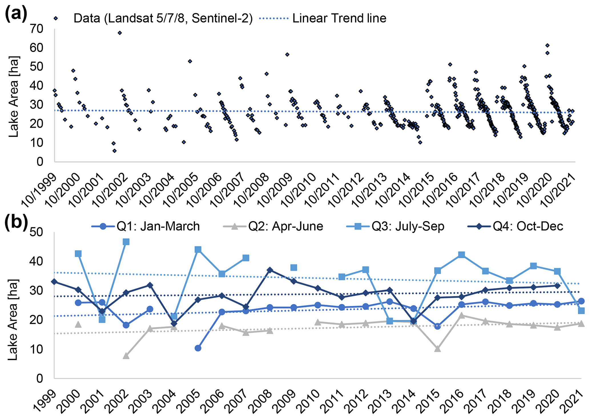
Figure A1 (a) Time series of Lac Kononi surface water area retrieved from Landsat 5, 7, and 8 as well as Sentinel-2 optical satellite imagery for the period 1 October 1999 until 30 September 2021 along with the linear trend line. (b) Annual average quarterly lake areas and associated linear trend lines. The location of Lac Kononi is indicated in Fig. 1.