the Creative Commons Attribution 4.0 License.
the Creative Commons Attribution 4.0 License.
 | 09 Sep 2022
Drainage reorganization induces deviations in the scaling between valley width and drainage area
Liran Goren
Onn Crouvi
Hanan Ginat
Eitan Shelef
The width of valleys and channels affects the hydrology, ecology, and geomorphic functionality of drainage networks. In many studies, the width of valleys and/or channels (W) is estimated as a power-law function of the drainage area (A), W=kcAd. However, in fluvial systems that experience drainage reorganization, abrupt changes in drainage area distribution can result in valley or channel widths that are disproportional to their drainage areas. Such disproportionality may be more distinguished in valleys than in channels due to a longer adjustment timescale for valleys. Therefore, the valley width–area scaling in reorganized drainages is expected to deviate from that of drainages that did not experience reorganization.
To explore the effect of reorganization on valley width–drainage area scaling, we studied 12 valley sections in the Negev desert, Israel, categorized into undisturbed, beheaded, and reversed valleys. We found that the values of the drainage area exponents, d, are lower in the beheaded valleys relative to undisturbed valleys but remain positive. Reversed valleys, in contrast, are characterized by negative d exponents, indicating valley narrowing with increasing drainage area. In the reversed category, we also explored the independent effect of channel slope (S) through the equation W=kbAbSc, which yielded negative and overall similar values for b and c.
A detailed study in one reversed valley section shows that the valley narrows downstream, whereas the channel widens, suggesting that, as hypothesized, the channel width adjusts faster to post-reorganization drainage area distribution. The adjusted narrow channel dictates the width of formative flows in the reversed valley, which contrasts with the meaningfully wider formative flows of the beheaded valley across the divide. This difference results in a step change in the unit stream power between the reversed and beheaded channels, potentially leading to a “width feedback” that promotes ongoing divide migration and reorganization.
Our findings demonstrate that valley width–area scaling is a potential tool for identifying landscapes influenced by drainage reorganization. Accounting for reorganization-specific scaling can improve estimations of erosion rate distributions in reorganized landscapes.
- Article
(9218 KB) - Full-text XML
-
Supplement
(1284 KB) - BibTeX
- EndNote


The width of channels and their hosting valleys controls river dynamics and functionality with far-reaching implications across a wide range of disciplines from flood hazards (e.g., Lóczy et al., 2009; Mashael Al, 2010; Sampson et al., 2015) to river ecosystems, river habitats (e.g., Beeson et al., 2018; Brussock et al., 1985; May et al., 2013; Sweeney et al., 2004), and hydrological modeling (e.g., Looper et al., 2012). Valley and channel width further plays a central role in landscape evolution (Amos and Burbank, 2007; Fisher et al., 2013; Hancock and Anderson, 2002). The relation between valley width, which subsumes channels, terraces, and floodplains, and other measures of valley morphology, including depth and fill thickness, is used to elucidate drainage evolution over geological timescales (e.g., Gibling, 2006; Schumm and Ethridge, 1994) and for inferring past climate changes (e.g., Dury, 1964; Hancock and Anderson, 2002; Marcotte et al., 2021) and tectonic variations (Giaconia et al., 2012). The channel width is a key component in landscape evolution for its control on the shear stress exerted by the flowing water, sediment transport capacity, and erosion rate (Whittaker et al., 2007b; Yanites et al., 2010). Particularly, many landscape evolution and hydrological models approximate the local erosion rate as a function of the channel stream power per unit channel width (Harbor, 1998; Magilligan et al., 2015).
The central role of valley and channel width across disciplines highlights the value of high-resolution width measurements, which could vary by several orders of magnitude within a single basin as well as across basins and landscapes (Schumm and Ethridge, 1994). Producing high-resolution field-based width measurement of channels and valleys is challenging and time-consuming, and in recent years a growing body of work has focused on developing tools for automatic width extraction based on remotely sensed data (e.g., Clubb et al., 2022; Fisher et al., 2013; Gilbert et al., 2016; Hilley et al., 2020; Monegaglia et al., 2018; Roux et al., 2015; Rowland et al., 2016). Although these tools represent a significant advancement in river research and management, they commonly focus on specific types of river morphology and require parameter calibrations, as well as human supervision (Fryirs et al., 2019; Golly and Turowski, 2017). Due to these limitations, in many cases, width of natural channels and valleys is estimated based on the widely recognized scaling relationships between valley width or channel width and fundamental basin fundamental basin properties such as discharge (or its proxy, drainage area), which could be relatively easily measured from digital elevation models (e.g., Lavé and Avouac, 2001; Wobus et al., 2006). Furthermore, channel width–drainage area scaling relationships are frequently used in landscape evolution models, for which channel width is implicitly parameterized based on the drainage area (e.g., Goren et al., 2014; Lague et al., 2014; Shobe et al., 2017; Yanites et al., 2013). However, studies that explored the channel width–drainage area scaling found that it is valid mostly under steady-state conditions but is less reliable when lithologic, climatic, and tectonic complexities are present in the landscape (Allen et al., 2013; Montgomery, 2004; Snyder and Kammer, 2008; Whipple et al., 2013; Yanites, 2018). Consequently, in such landscapes, a more complex scaling involving channel width, area, and slope was shown to be more applicable (Finnegan et al., 2005). While the influence of tectonic, climatic, and lithologic changes on valley and channel width has been extensively explored (e.g., Allen et al., 2013; Keen-Zebert et al., 2017; Marcotte et al., 2021), the effects of drainage reorganization, which imposes drainage area transiency, were mostly overlooked. The current study targets these effects by exploring valley and channel width scaling under transient conditions that emerge from processes of drainage reorganization.
1.1 Width–area scaling in channels and valleys
The common approach for channel width estimation relies on the seminal work of Leopold and Maddock (1953), who used empirical data to establish a power-law relation between the channel width, W [m], and discharge, Q [m3 s−1]. Combined with the documented correlation between discharge and drainage area, A [km2] (e.g., Dunne and Leopold, 1978), the scaling between channel width and drainage area is often expressed as
Leopold and Maddock's relation (Eq. 1) was established for alluvial rivers, where d was found to be ∼ 0.5. A similar scaling was later reported for bedrock rivers, with an exponent that typically ranges 0.3–0.6 (Kirby and Ouimet, 2011; Montgomery and Gran, 2001; Snyder et al., 2003; Tomkin et al., 2003; Whitbread et al., 2015; Yanites et al., 2010). The exponent's range was mostly attributed to differences in channel bank properties, with more erodible and/or fractured banks widening faster than resistant and intact banks (Spotila et al., 2015; Whitbread et al., 2015; Wohl and Achyuthan, 2002; Wohl and David, 2008). Other studies invoked climatic variations and anthropogenic disturbances to explain variations in the d exponent (Bertrand and Liébault, 2019; Faustini et al., 2009; Snyder et al., 2003).
Although Eq. (1) is commonly used as an empirical relation, it is consistent with process-based theory. Channel widening is attributed to lateral bank erosion induced by particles impacting the channel wall (Li et al., 2020; Turowski, 2018) and is governed by the mechanical properties of the bedload and the channel banks, the channel geometry, and the volume and trajectory of the bedload particles (e.g., Finnegan and Balco, 2013; Li et al., 2020; Yanites, 2018). Considering these controlling parameters, Turowski (2018) developed a model relating bedrock channel width to sediment supply, vertical erosion rate, and bank properties. Under a spatially uniform erosion rate and steady-state conditions, Turowski's model predicts that the channel width is a power-law function of the drainage area, consistent with the form of Eq. (1).
Valley widening occurs when the channel migrates and abuts the valley wall, enabling particles from the channel to erode the valley wall. The effectiveness of valley widening is thus controlled by the frequency at which the channel abuts and erodes the valley wall; this depends on the valley width, channel width, and channel mobility within the valley, which increases with sediment flux (Clubb et al., 2022). Despite the different processes that underlie the widening of channels and valleys, empirical observations suggest that the relation between the valley width and drainage area follows a power-law scaling similar to Eq. (1) (Beeson et al., 2018; Brocard and van der Beek, 2006; Clubb et al., 2022; Langston and Temme, 2019; Langston and Tucker, 2018; May et al., 2013; Schanz and Montgomery, 2016; Snyder et al., 2003; Tomkin et al., 2003). However, the reported range of the exponent d is significantly wider in valleys, ranging between negative values of −0.13 (Clubb et al., 2022) and positive values as high as 1.18 (Beeson et al., 2018). Here, too, the exponent range was attributed to differences in the properties of valley-bounding rocks (Brocard and van der Beek, 2006; Keen-Zebert et al., 2017; Langston and Temme, 2019; Schanz and Montgomery, 2016) or, in some high-relief landscapes, to the spatial distribution of deep-seated landslides that can cause local recession of the valley walls and, at times, dam the valley and cause upstream aggradation and widening (Beeson et al., 2018; Clubb et al., 2022; May et al., 2013).
1.2 Width–area–slope scaling relation in channels and valleys
While the applicability of the simple power-low scaling between channel width and drainage area (Eq. 1) was demonstrated in many settings (Montgomery and Gran, 2001; Whipple et al., 2013; Whitbread et al., 2015; Wohl and David, 2008), field observations show that it is not applicable across all landscapes. Notably, the scaling was demonstrated to fail along areas of localized gradient in rock uplift, e.g., due to local faulting or folding (Allen et al., 2013; Amos and Burbank, 2007; Kirby and Ouimet, 2011; Lavé and Avouac, 2001; Yanites et al., 2010), along channels with alternating lithologies (Montgomery, 2004; Spotila et al., 2015), and in channels with transient morphologies due to temporal changes in rock uplift rate (Whittaker et al., 2007a, b; Yanites, 2018). Finnegan et al. (2005) developed a model for the case of a channel that crosses terrain with variable rock uplift rates. Adopting Manning's equation (Manning et al., 1890) and assuming a constant bankfull width-to-depth ratio along the channel, Finnegan's model predicted that the channel width depends on both the drainage area, as in Eq. (1), and the channel slope, S [m m−1]:
The exponents b and c in Finnegan's model were calculated to be 0.38 and −0.19, respectively, which are values that were later supported by observations in various field studies (Finnegan et al., 2005; Kirby and Ouimet, 2011; Spotila et al., 2015; Wright et al., 2022). In studies of transient channel adjustment to changing tectonic forcing, Whittaker et al. (2007a) and Attal et al. (2008) found that a greater absolute value of −0.44 for c produces better fits for their field observations. The slope dependency in Eq. (2) is consistent with the approach of Turowski (2018) in scenarios in which transient conditions are considered, such that the ratio of sediment flux to channel vertical erosion becomes slope-dependent.
The significance of including channel slope as a controlling parameter in Eq. (2) depends on the covariance between slope and drainage area. In steady-state drainage networks with uniform lithology, climate, and uplift rates, the channel slope, S, and the drainage area, A, covary through a power-law relation (Flint, 1974). Therefore, in these cases, the slope can be substituted by the drainage area, and Eq. (2) reduces to the form of Eq. (1). In contrast, the cases in which Eq. (2) was found to be a better predictor for channel width (Finnegan et al., 2005; Kirby and Ouimet, 2011; Spotila et al., 2015; Whittaker et al., 2007a; Wright et al., 2022) are those in which S and A do not covary.
A theory that relates valley width to drainage area and channel slope in the form of Eq. (2) was provided by Brocard and van der Beek (2006) in settings with alternating alluvial and bedrock sections. In their conceptual model, the inclusion of the channel slope, S, as a controlling parameter on the valley width emerges from spatial and temporal variations in the environmental conditions. For example, the channel steepness can serve as a proxy for lithological variations that set the mode of valley widening at different reaches. Alternatively, in scenarios of a channel incising into a wide flat valley, increased channel slope is often associated with bank steepening, resulting in bank slumping that forms a narrower valley within the preexisting valley bottom. Despite this appealing reasoning, to the best of our knowledge, so far Eq. (2) has not been used to predict valley width in any particular field setting.
1.3 Drainage reorganization and width scaling of valleys and channels
Drainage reorganization is widely recognized as an important process affecting the evolution of fluvial systems (e.g., Bishop, 1995; Fan et al., 2018; Harel et al., 2019; Prince et al., 2011; Willett et al., 2014). Reorganization occurs when drainage divides shift through time (Bishop, 1995; Davis, 1889), change basin geometry, and consequently induce changes in the distribution of discharge and drainage area along channels (e.g., Menier et al., 2017; Pechlivanidou et al., 2019). Referring to the width–area scaling in Eq. (1), addition or reduction of the drainage area is expected to result in channel and valley widening or narrowing, respectively. However, while drainage reorganization is capable of inducing relatively rapid drainage area changes, i.e., following river capture or repeated stochastic events (Shelef and Goren, 2021), width adjustment of channels and valleys most likely requires longer timescales (Brocard and van der Beek, 2006; Wright et al., 2022). Studies that measured channel widths in drainages that experienced recent anthropogenic drainage area perturbations reported ongoing width variations that prevailed for several decades (e.g., Jones, 2018; Snyder and Kammer, 2008). Based on a theoretical model, Turowski (2020) postulated that the timescale of channel width adjustment to discharge perturbations is of the order of thousands of years. For valleys, the time gap between the change in drainage area and width adjustment is expected to be even longer, most likely of the order of tens of thousands of years (Hancock and Anderson, 2002; Langston and Tucker, 2018), because valley width represents the channel location integrated over long periods (Schumm and Ethridge, 1994; Tomkin et al., 2003).
Although the potential scaling deviation following reorganization is highly consequential for fluvial landscape functionality, the effects of reorganization on fluvial channel and valley width scaling have not yet been evaluated. We hypothesize that this scaling, particularly that of the valleys, expresses the delayed response of width adjustment to drainage area changes following reorganization. Accordingly, the coefficient and exponent values that relate drainage area with valley width in reorganized drainages could meaningfully deviate from drainages that did not experience reorganization.
To test this hypothesis and to evaluate the effect of reorganization on width–area scaling of valleys and channels, we analyzed and compared the geometry of reorganized and undisturbed drainages in the southern Negev desert, Israel, where drainage reorganization is well-established by field observations (Avni et al., 2000; Ginat et al., 2000, 2002; Harel et al., 2019). In the current analysis, we aim to (i) explore if and how the scaling between valley width and drainage area in Eq. (1) varies between reorganized and non-reorganized drainages and among drainages that experienced different modes of reorganization. (ii) In cases when drainage area and slope do not covary, we study the independent slope influence on valley width scaling following Eq. (2). (iii) We compare the adjustment of channel width relative to valley width following reorganization and (iv) examine landscape evolution implications of the valley and channel width scaling in reorganized drainages.
2.1 Geologic and geomorphic setting
We explore channel and valley width scaling along ephemeral drainage networks that incise into the southeastern Negev Highlands, Israel (Fig. 1). The highlands are bounded to the east by ∼ 400–600 m high cliffs that rise above the Arava Valley, which is part of the transtensional Dead Sea plate boundary with a rift-like structure that stretches between the Dead Sea and the Gulf of Aqaba (Garfunkel, 1981; Garfunkel, 2014, Fig. 1a, b).
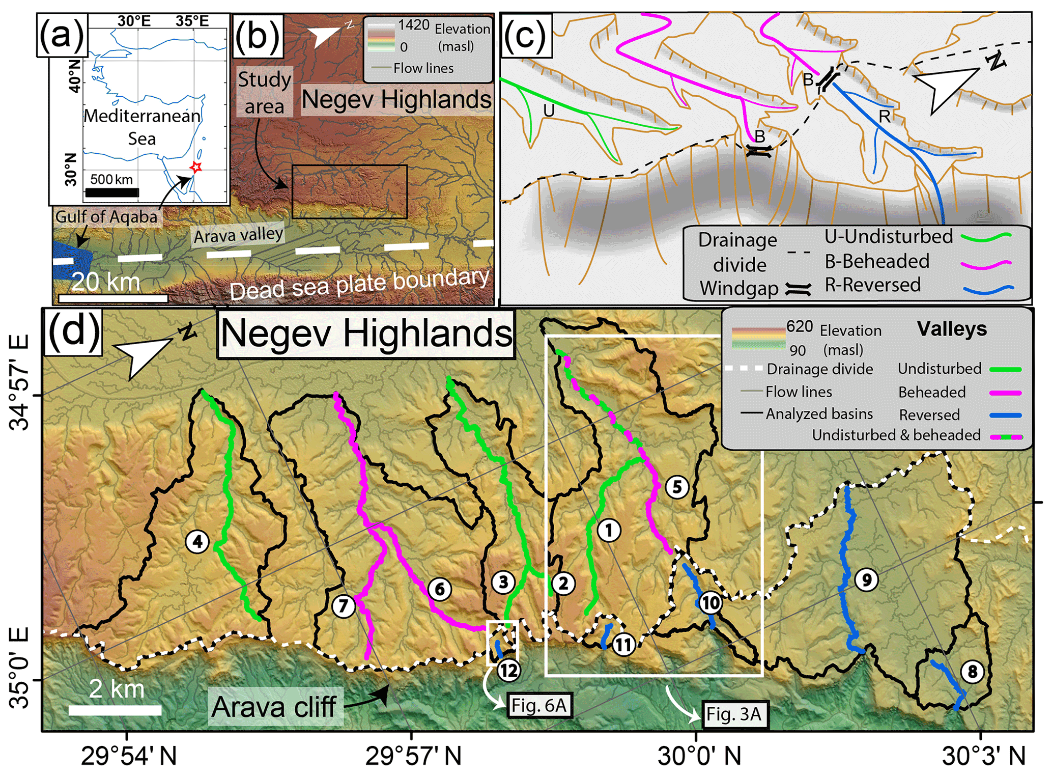
Figure 1(a) Orientation map with coastlines (blue) showing the study area location (red star). (b) Shaded elevation map, illustrating the regional rift morphology along the plate boundary (dashed white line) adjacent to the study area (black rectangle). The maps in (b) and (d) are based on the TanDEM-X 0.4 arcsec DEM (Wessel, 2016). (c) A simplified sketch of valley categorization in the study area: undisturbed valleys (green, “U” tag) are valleys that do not intersect the cliff and are minimally affected by drainage reorganization. Beheaded valleys are valleys that were beheaded due to cliff retreat or drainage reversal (pink, “B” tag), and reversed valleys (blue, “R” tag) that presently flow toward the cliff are commonly recognized by their barbed tributaries, which join the main channel at a >90∘ angle. (d) A shaded elevation map of the study area, illustrating the drainage divide (white dashed line) between the Negev Highlands and the Arava Valley. The basin boundaries (black lines) are defined by the valley section's outlet. Encircled numbers refer to the valley serial numbers in Tables 1 and 2.
The main drainage divide in the study area separates steep east-flowing basins that drain across the cliff toward the Arava Valley from west-flowing, low-relief basins that flow on the Negev Highlands (Fig. 1b–d). The lithology exposed along the highland valleys consists primarily of Cretaceous limestone and dolomite strata (Ginat, 1991). The climate is hyper-arid with average annual precipitation of ∼<50 mm (Bitan and Rubin, 1991), typically generating one to a few flash-flood events per year. These climatic conditions generally persisted through most of the Pleistocene (Amit et al., 2006, 2011), except for short episodes of wetter conditions (Ginat et al., 2018; Vaks et al., 2013).
The eastern Negev desert has been experiencing ongoing fluvial reorganization since the late Miocene (Avni et al., 2000, 2012). Before the development of the Arava Valley, rivers that originated in the Jordanian highlands, east of the Arava Valley, flowed westward, crossing the plate boundary along the Negev Highlands towards the Mediterranean (Garfunkel and Horowitz, 1966; Zilberman and Calvo, 2013). Since the Miocene, tectonic activity along the Dead Sea plate boundary has formed the Arava Valley, which gradually became a prominent base level. Consequently, during the Plio-Pleistocene, several large-scale capture events redirected major drainage systems in the Negev toward the central Arava Valley (Avni et al., 2000; Ginat et al., 2000, 2002; Guralnik et al., 2010). Field observations and a regional χ analysis (a morphometric parameter used to approximate the stability of drainage divides; Willett et al., 2014) suggest that the regional divide between the Arava Valley and the Negev Highlands is still actively migrating westward (Harel et al., 2019).
2.2 Categories and characteristics of valleys in the study area
To explore the effects of drainage reorganization on the valley width scaling relations, we analyzed 12 valley sections associated with different drainage reorganization categories. All sections are located adjacent to the Negev–Arava drainage divide (Fig. 1d), resulting in relatively small drainage areas of 0.2–14.2 km2. The valleys are incised into bedrock, generating relief of several tens of meters between the valley bottoms and the highlands' flat interfluves. The valleys were classified into three categories based on the association of the valley with the Arava cliff (Fig. 1c, d), the morphology of the valley section (Fig. 2), and additional supporting field observations. The three categories are as follows.
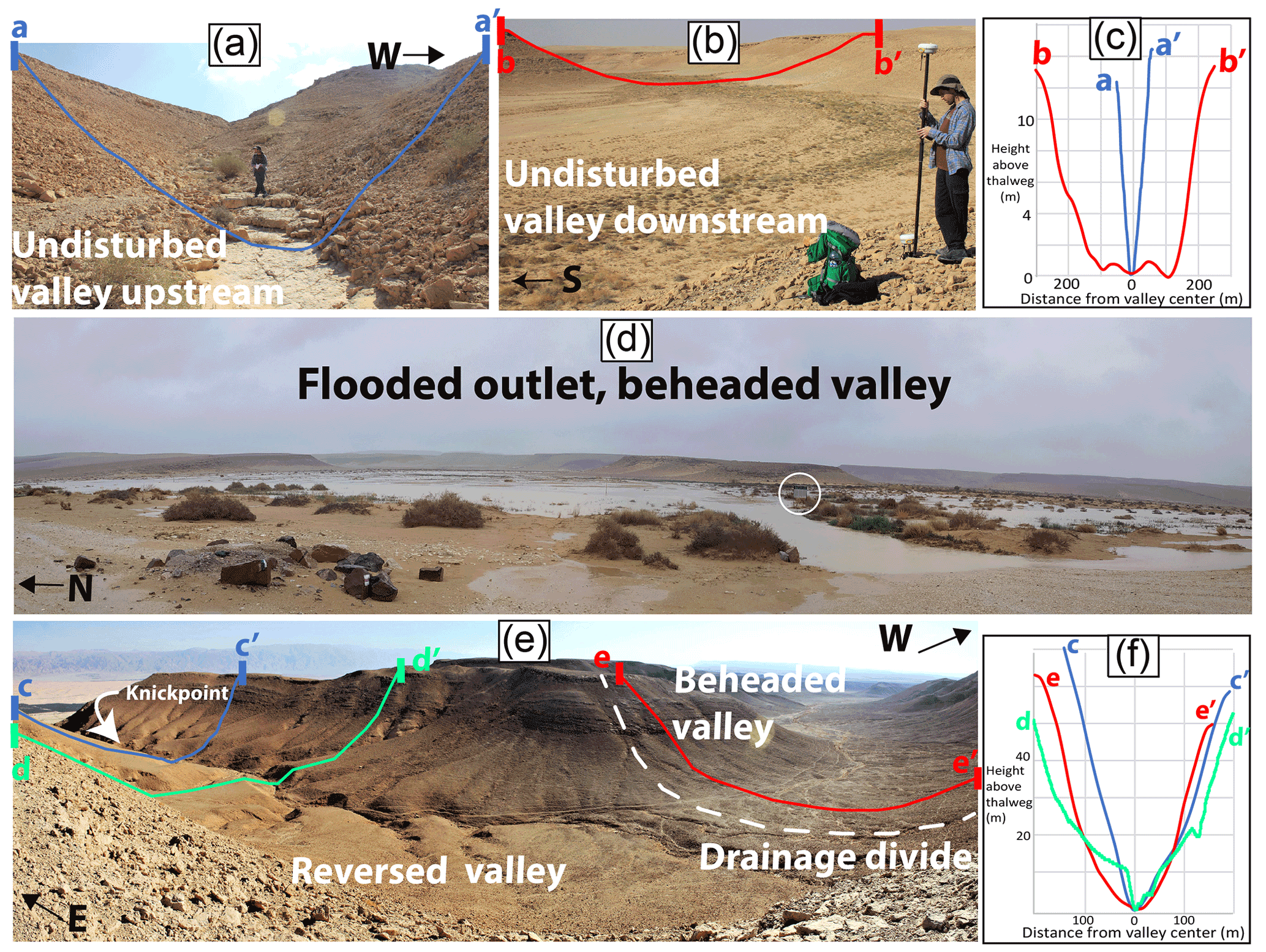
Figure 2Field photos and valley transects of valley sections in the study area. (a, b) Upstream and downstream segments of undisturbed valleys (a and b, respectively). The drainage area in panel (a) is 0.08 km2 and in panel (b) is 1.85 km2. Blue and red lines (a–a' and b–b', respectively) mark the cross-section profiles shown in panel (c). (c) Transects of a–a' and b–b'. Note the V-shaped transect near the valley head relative to the trapezoid morphology of the downstream section. (d) Flooded valley bottom at the outlet of two beheaded valleys (6 and 7) after an intense rain event in February 2020. A sign ∼ 1.5 m wide is encircled for scale. (e) Panorama of reversed and beheaded valleys (valleys 12 and 6 in Table 1 and Fig. 1d), as well as the confined, flat wind gap between them. The c–c' transect (blue) was measured near the knickpoint at the edge of the reversed section; d–d' (green) follows the terraces representing the paleo-valley and the channel that incises into them, and e–e' (red) was measured close to the wind gap on the beheaded side. (f) Cross-sections of transects c–c', d–d', and e–e', emphasizing the difference between the U-shaped transect near the wind gap (e–e'), the V-shaped channel profile incised into the U-shaped valley terraces (d–d'), and the V-shaped valley transect above the knickpoint (c–c').
-
Undisturbed valleys (n=4) are westward-flowing valley sections whose headwaters are adjacent to the cliff line and are not meaningfully beheaded. In some cases, field evidence indicates that some portions of the drainage area along the low-relief interfluves were lost due to divide migration associated with cliff receding. Yet, the receding cliff does not intersect the incised portion of the valleys; therefore, these valleys are referred to as “undisturbed”. In these valleys, the low-order (sensu Strahler) incised segments are characterized by a V-shaped morphology (Fig. 2a, c) with a bedrock valley bottom that is several meters wide. Farther downstream, typically at a distance less than 1 km from the valley head, the valley bed becomes alluviated, and its width increases to tens of meters. Higher-order valleys widen downstream at slower rates than low-order valleys and typically have a trapezoid cross-section with a sediment-filled flat valley bottom and steep valley walls (Fig. 2b–d). In the undisturbed and beheaded categories (below), the entire valley is typically occupied by a low-relief, braided, and dynamic channel system. Field observations of the fully flooded valley bottom during large rainstorm events (Fig. 2d) suggest that the formative flow width is the entire width of the valley bottom.
-
Beheaded valleys (n=3) are west-flowing sections whose headwaters were beheaded. Beheading is indicated by a wind gap, i.e., a flat, valley-confined drainage divide located along the cliff or shared with a reversed valley (described below), indicating the truncation of an incised paleo-valley that likely drained a larger area. Close to the wind gap, the beheaded valleys are characterized by a U-shaped cross-section (e.g., Figs. 1c, 2e–f, 3a, and 6a), likely controlled by the concave profiles of side colluvial aprons. West and downstream from the wind gap, beheaded valleys become indistinguishable from the undisturbed valleys with the trapezoid-shaped cross-section. Valley beheading is associated with either the receding cliff and its coinciding divide or with localized divide migration within the valley as part of a reversal process on the opposing side of the wind gap (e.g., Bishop, 1995; Harel et al., 2019; Shelef and Goren, 2021). The beheaded valleys have a valley bed morphology similar to the undisturbed category; thus, the formative flow width of the beheaded valleys is the entire width of the valley bottom.
-
Reversed valleys (n=5) host east-flowing channels that reversed their drainage direction (Bishop, 1995) from west to east. These valleys are bounded between a wind gap on the west side and a knickpoint on the east, where the channel flows across the cliff (e.g., Figs. 2e, 3a and 6a). Harel et al. (2019) identified these sections as reversed drainages based on the presence of barbed tributaries and west-grading terraces that record the antecedent valley gradient, which is opposite to the present-day channel's drainage direction. The reversed valley sections share wind gaps with beheaded valleys, indicating that they were part of an antecedent west-flowing drainage (Harel et al., 2019). The two northern reversed valleys (8 and 9 in Fig. 1d) initiate in an E–W-trending strike valley which dictates a wide wind gap (>500 m, Ginat, 1997), whereas downstream from the divide they exhibit trapezoid cross-sections. In the three other valleys, the wind gap is U-shaped, and downstream the channel incises into alluvial–colluvial valley fill, creating cut terraces and forming a V- or box-shaped channel cross-section within the broader valley (e.g., transect d–d' in Fig. 2e, f). In most cases, close to the knickpoint where the channel crosses the cliff, it incises into bedrock, and the valley cross-section changes to a V-shaped morphology (e.g., transect c–c' in Fig. 2e, f).

Figure 3Valley width measurements and regression-based models for valleys 1, 5, and 11 from Fig. 1d and Tables 1 and 2. (a) A valley bottom polygon (black) overlies a shaded elevation map based on the TanDEM-X 0.4 arcsec DEM (Wessel, 2016). Green, pink, and blue lines represent transects of undisturbed, beheaded, and reversed valley sections, respectively. Dashed lines represent measurements at valley sections downstream of confluences between undisturbed and beheaded valleys. The reversed valleys extend between the main drainage divide (dashed white curve) and knickpoints (white boxes located at the cliff–flowline intersections). (b) Linear regression fitted lines from log-transformed valley width and drainage area for the undisturbed, beheaded, and reversed valleys 1, 5, and 11, respectively. The dashed lines represent 95 % confidence bounds. The equations in the bottom right are the linear models' kc coefficients and d exponents. (c) Multivariate regression results with the associated kb coefficient as well as b and c exponents for the reversed valley 11. The 95 % confidence interval is represented by error bars.
We studied the effect of reorganization on the width scaling of valleys by exploring the coefficients and exponents that control valley width variation following Eqs. (1) and (2). Valley width–drainage area scaling, based on Eq. (1), is explored for all valley sections in our study area, and the role of the slope is explored through Eq. (2) only for the reversed sections that generally show poor correlations between slope and drainage area. In one reversed section, we focus on the scaling between channel width, drainage area, and channel slope that emerges through Eq. (2).
3.1 Drainage area and slope extraction
Elevation data were derived from TanDEM-X (Wessel, 2016) with 0.4 arcsec resolution (∼ 11.6 m px−1 in the field area). The drainage area was extracted from a flow accumulation raster, computed using a D8 flow-routing algorithm (O'Callaghan and Mark, 1984). The threshold drainage areas used for defining the flow network are specified in Table S1 in the Supplement. The channel slope used for exploring slope–area relations as well as channel and valley width predictions following Eq. (2) was estimated along the flow network (thalweg) by using the slope of a linear regression between elevation and distance over a centered 7 px running window.
3.2 Valley width measurements
To compute the coefficients and exponents of Eqs. (1) and (2) that best fit the geometry of valley sections in the study area, we extracted the valley widths along the analyzed valley sections. In the undisturbed and beheaded categories, the valley width refers to the flat valley bottom that is fully flooded during formative floods, while in the reversed category the valley width typically includes terraces that preserve former levels of the valley bottom (Harel et al., 2019). Unlike the upstream drainage area and slope, which are derived through relatively simple calculations over the digital elevation model (DEM), defining and extracting the valley width based on a DEM is not straightforward and requires a tailored procedure (Clubb et al., 2017, 2022; Golly and Turowski, 2017; Hilley et al., 2020; Roux et al., 2015; Rowland et al., 2016; Sechu et al., 2021). Particularly, the location and orientation of valley width measurements require caution because the width is often not well-defined in proximity to side tributaries and valley bends (Beeson et al., 2018; Clubb et al., 2022). To overcome these challenges, we developed a semi-automatic approach for optimal measurements of valley width.
Valley width was measured by applying two consecutive operations. First, a polygon representing the valley bottom is extracted, and second, valley width is measured over the valley bottom polygon at optimal points (Fig. 3a). The first step is achieved by applying the ArcGIS plugin VBET – “valley bottom extractor tool” (Gilbert et al., 2016). VBET identifies valley boundaries based on user-defined slope thresholds, representing the transition from the valley bottom to the hillslope. This method is particularly suited for valley morphologies wherein the valley bottom can be easily distinguished from the valley walls based on a distinct slope break, which is the case in most of the studied valley sections. VBET parameters used for the current analysis are described in Table S1 in the Supplement. Importantly, these parameters were fitted to each basin (each including one or two sections) separately by an iterative process of visually comparing the valley bottom polygons against 0.5 m px−1 aerial orthophotos and fine-tuning the parameters to achieve the best visual fit. In six basins, this procedure was not sufficient to achieve a satisfying fit between the VBET polygon and the orthophoto, mainly due to local DEM inaccuracies. In these cases, the polygons were manually edited to correct local mismatches based on the orthophotos, available topographic data, and field observations. In five of the edited polygons, the area difference between the original and the edited polygons was <5 %; in one case, the area difference was 10 % (Table S1 in the Supplement). Shapefiles of the polygons before and after manual editing are available in the Supplement (Harel, 2022a).
Valley width measurements over the VBET polygons were achieved by applying an ArcGIS-based algorithm that identifies points that are sufficiently far from bends and confluences and are located along the valley centerline (Harel, 2022b). In these optimal locations, valley transects are taken perpendicular to the centerline, whose length represents the valley width. The final output is a set of pixels located at intersections between the thalweg and the valley transects, which are assigned with valley width, drainage area, and slope values (e.g., Fig. 3a). The algorithm is described in detail in Sect. S1 and Figs. S1–S5 in the Supplement.
3.3 Regression analysis
As a preliminary step to explore valley width scaling, the covariance between slope S [m m−1] and drainage area A [km] was quantified using linear regression over binned log-transformed values (e.g., Wobus et al., 2006). For all valley sections, the best-fit values of kc and d in Eq. (1) were calculated by using a least-squares linear regression over log-transformed W [m] and A [km2] (e.g., Fig. 3b). We used units of square kilometers [km2] for drainage area to facilitate direct comparison with prior studies that conducted a similar analysis using these units (e.g., Clubb et al., 2022; Langston and Temme, 2019; Schanz and Montgomery, 2016; Tomkin et al., 2003). In the reversed category, the slope and area do not always covary; hence, in this category we used multivariate least-squares linear regression over log-transformed W [m], A [km2], and S [m m−1] to find the best-fit values of kb, b, and c in Eq. (2) (following Attal et al., 2008; Spotila et al., 2015) (e.g., Fig. 3c). In the regressions used for Eqs. (1) and (2), the data were not binned.
3.4 Detailed analysis of channel and valley width
In contrast to the undisturbed and beheaded categories, in the reversed category, the valley and the channel are decoupled. In this category, we examined how fitting the valley width compared to the channel width affects the predictors kb, b, and c in Eq. (2). Valley 12 (Fig. 1d and Tables 1 and 2) is a thoroughly surveyed site (Harel et al., 2019) that was chosen for this analysis. The channel parameters are based on a 15 cm px−1 DEM and a 3 cm px−1 orthophoto generated using a structure from motion (SfM) algorithm over drone-acquired aerial photos (80 % overlap). Here, the sub-meter-scale topography of the high-resolution DEM inhibited the VBET tool from discriminating the channel bottom precisely, and therefore the channel bottom polygon was delineated manually based on the 15 cm px−1 DEM and the 3 cm px−1 orthophoto. Then, the valley width measurement algorithm described in Sect. 3.2 was applied over the channel polygon. The drainage area and elevation data were extracted from the 15 cm px−1 DEM. The slope was calculated following the procedure described in Sect. 3.1, with a running window of 541 px, such that the length of the along-flow distance covered by the window was comparable to that used for the valleys. Finally, the best-fit kb, b, and c values were calculated using a multivariate least-square linear regression, as described in Sect. 3.3.
3.5 Validations and errors in the measurements and model
The main potential sources of valley width measurement errors originate from the DEM horizontal resolution, R (∼ 11.6 m2 px−1), and the relative vertical accuracy (∼ 2 m, Wessel, 2016). To incorporate the uncertainty stemming from the horizontal resolution of the DEM, we assigned each valley width measurement a constant error, evaluated as .
To independently explore the effect of inaccuracies in the DEM on the final valley width measurements, seven valley transects were measured with a differential GPS (DGPS). The valley bottom was extracted from the transects by applying the same criteria used to identify the slope break that was applied in VBET to that basin. The DEM-based and DGPS-based valley width measurements and their relations are shown in Fig. S6 and in Table S2 in the Supplement. The differences between the DEM-based measurements relative to the DGPS-based measurements range 2–20 m and are scale-independent. The percent deviation between the measurements is <0.3 %, except for the narrowest valley, for which ∼3 m difference between the DEM and the DGPS-based measurements yielded a percent deviation of ∼25 %. Overall, the mean percent deviation is 3.7 %, and the RMSE is 13 m (whereas the mean valley width of the seven transects is 110 m), which is smaller than the resolution-associated error of .
4.1 Slope area correlation
The slope–area relation of the studied valley sections is presented in Fig. S7 in the Supplement. The R2 vales of the slope–area regressions in the undisturbed and beheaded valleys range from 0.68 to 0.93. In the reversed valleys, the R2 of two valley sections is ∼ 0.5, and the R2 of the other three reversed valley sections is <0.14. As mentioned in Sect. 1.2, when slope and area strongly covary, Eq. (2) reduces to the form of Eq. (1). For that reason, while the valley width–drainage area scaling (Eq. 1) is computed for all valley categories, Eq. (2) is applied only for the reversed valley sections where the slope–area covariance is low.
4.2 Valley width–drainage area scaling
The best-fit coefficients and exponents of the valley sections, their 95 % confidence intervals, and the R2 for the regression are presented in Table 1 and Fig. 4. P values of the predictors and the least-square regressions are provided in Table S3 in the Supplement. The regressions are depicted in Fig. S8 in the Supplement.
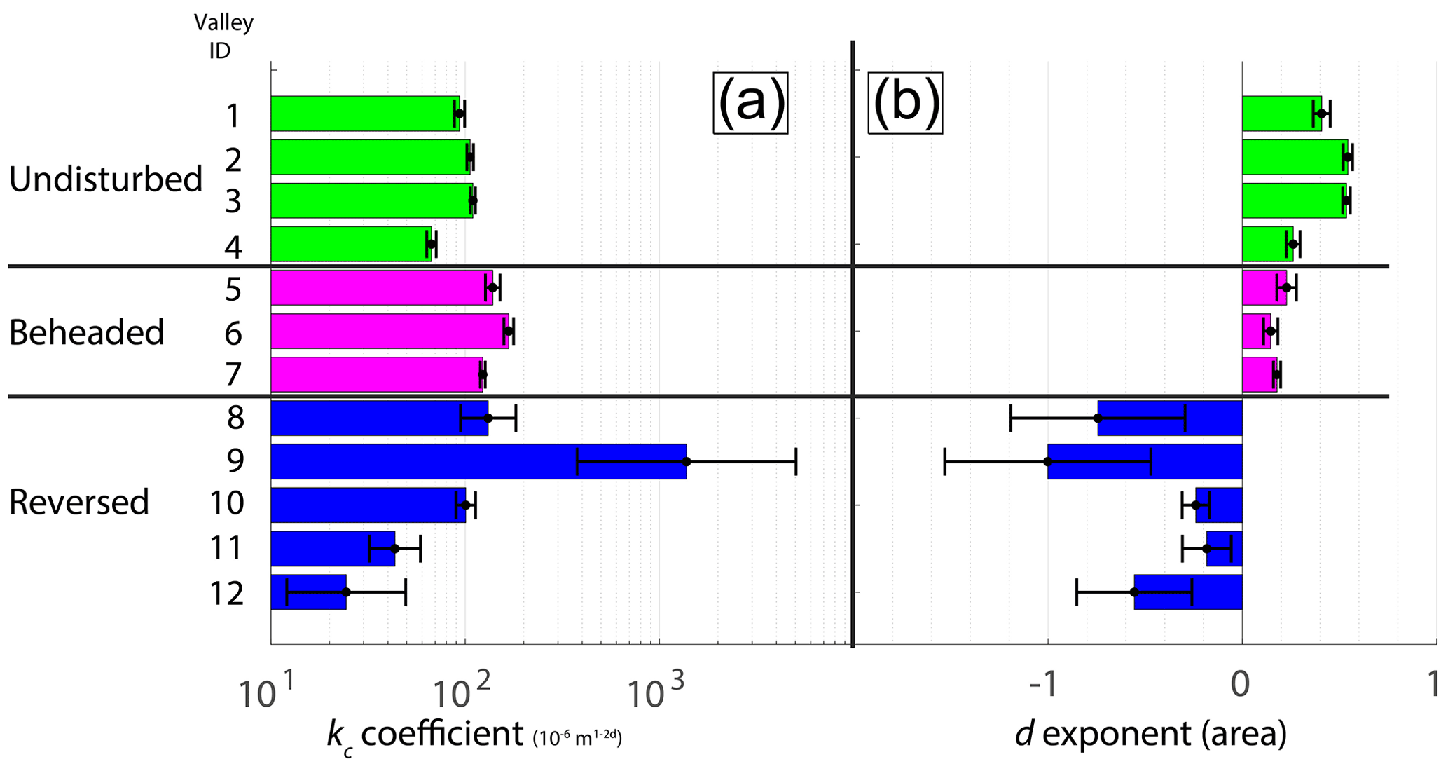
Figure 4Bar plots of the kc and d values (a, b, respectively) for valley sections of the categories defined in Fig. 1c. The error bars represent the 95 % confidence interval. Unlike the kc values, which lack a clear trend, the values of the d exponent (b) fall within a distinct range for each valley category. Note the log scale of the x axis in panel (a).
Table 1Regressions for Eq. (1), W=kcAd, applied to all valley sections.
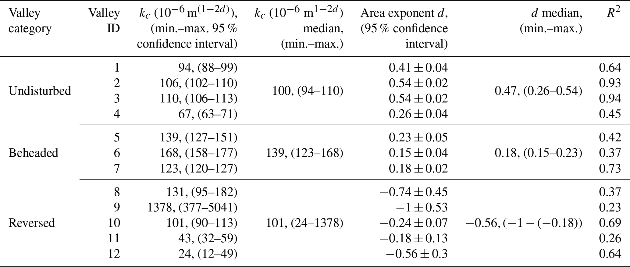
The least-square regression results reveal unique ranges of the drainage area exponents, d, for each predefined valley category (Fig. 4b). The undisturbed valleys are characterized by the highest exponents, ranging from 0.26 to 0.54, whereas the d exponents of the beheaded valleys are lower at 0.15–0.23. Uniquely, the reversed valleys have negative d exponents ranging from −0.18 to −1, indicating that in this category, the valleys narrow with increasing drainage area.
Unlike the d exponent values, the kc coefficients are nonunique for the different valley categories (Fig. 4a). The values of the kc coefficient, which represents a valley width at A=1 [km2], range from 94 to 110 (10−6 m1−2d) in the undisturbed valleys, which differs from the range of the beheaded valleys category of 123–168 (10−6 m1−2d). The kc coefficient values for the reversed valleys show large variability across 3 orders of magnitude ranging between 24 (10−6 m1−2d) and 1378 (10−6 m1−2d).
The performance of the power-law model (Eq. 1) was evaluated through the value of R2. In the undisturbed and beheaded categories, R2 ranged 0.37–0.94. In the reversed valleys, two valleys show R2 values of 0.64 and 0.69, and the three other valleys exhibited lower values of 0.23–0.37 (Table 1). The W–A relations are statistically significant for all valleys (α=0.05, Table S3 in the Supplement).
4.3 Valley width–drainage area–slope scaling in the reversed category
The results in Sect. 4.1 demonstrate that most reversed valleys are characterized by a poor correlation between slope and drainage area. Therefore, in this category, Eq. (2) may yield a better prediction for the valley width as a function of both the drainage area and slope. In Table 2 and Fig. 5, we present the results of this multivariate regression, including 95 % confidence intervals and adjusted R2. P values of the predictors and of the multivariate regressions are provided in Table S4 in the Supplement.
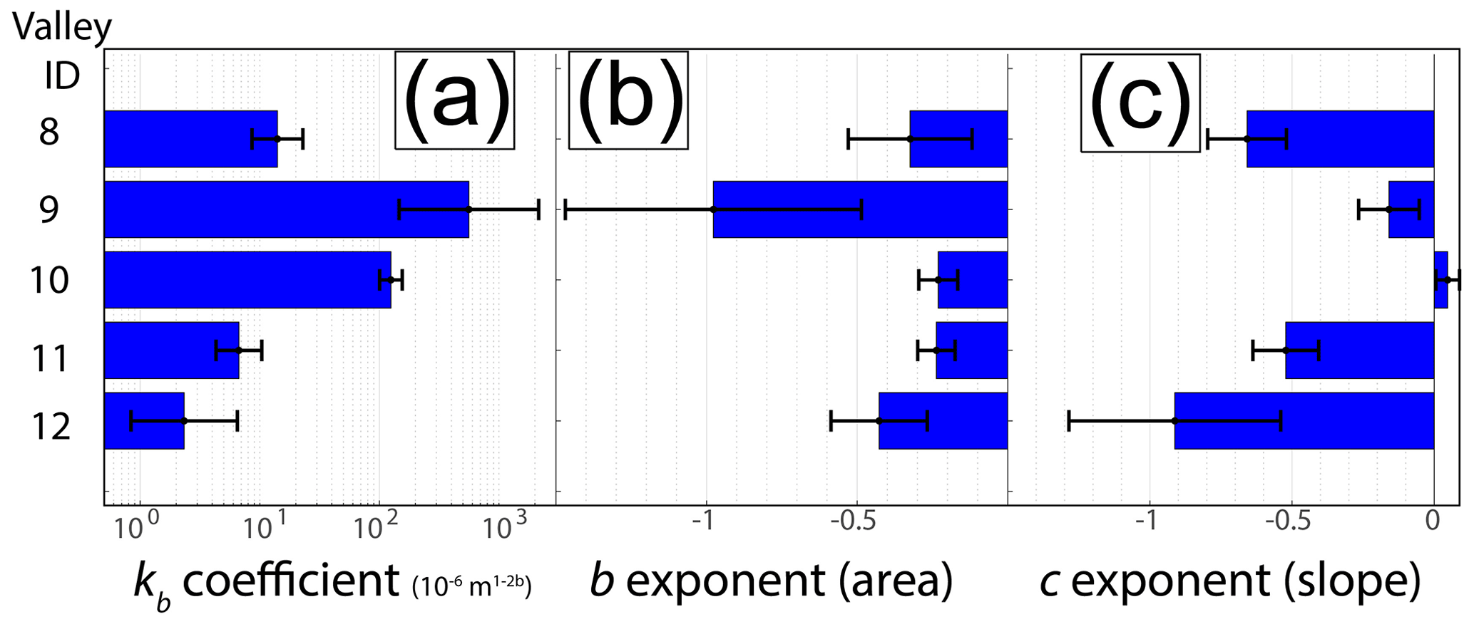
Figure 5Bar plots of the kb coefficient as well as b and c exponents in Eq. (2) for the reversed valley category (panels a, b, and c, respectively), fitted by multivariate regression. Error bars represent the 95 % confidence interval. The kb values show large variability. The area exponents, b, are generally less negative than the d exponents fitted to Eq. (1) in Table 1 and Fig. 4. Except for valley 10, the slope exponents c have negative values. In valleys 8, 11, and 12, the c exponent is more negative than the area exponent, b, reflecting the key role of slope in reversed valley width prediction. Note the log scale of the x axis in panel (a).
Table 2Regressions for Eq. (2), W=kbAbSc, applied only to the reversed valley sections.
a Adjusted R2 is used here for conservativeness. b Predictor P value >0.05. See Table S4 in the Supplement.
The results of the multivariate regression based on Eq. (2) demonstrate that in the reversed valley sections, the drainage area exponent, b, remains negative and is within the range of −0.98 to −0.23, similar to the drainage area exponent d computed based on Eq. (1) (Fig. 5b). The kb coefficients are between 2 and 561 (10−6 m1−2b) (Fig. 5a). The values of the slope exponent, c, are negative, between −0.91 and −0.16, except for valley 10, where the exponent is about zero (Fig. 5c). With the exception of valley 9, the adjusted R2 of the model is 0.74–0.92. Overall, all the adjusted R2 values based on Eq. (2) are higher than the standard R2 obtained based on Eq. (1).
4.4 Comparing valley width and channel width in a reversed drainage
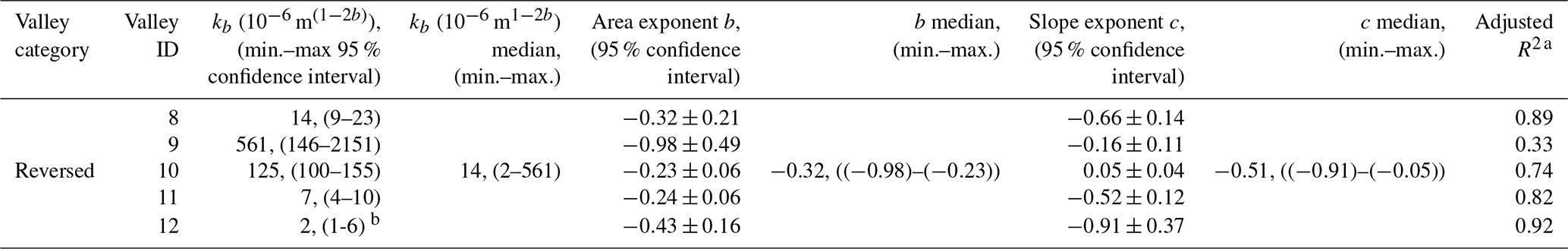
To explore the effect of the drainage area and slope on the width of the channel vs. the width of the valley in a reversed valley section, where the valley and the channel are decoupled, we extracted the predictors kb, b, and c in Eq. (2) for channel width in reversed valley 12 (Table 2, Fig. 6). The channel in valley 12 initiates east of the wind gap and incises into the erodible valley fill, where it merges with short side tributaries. Farther downstream, it merges with a barbed tributary that joins the valley from the north (Fig. 6a). At the barbed tributary junction point, the reversed channel is incised ∼ 15 m below the surface of the antecedent valley bottom. Approximately 160 m farther downstream, bedrock is exposed at the base and the north bank of the channel. The channel traverses the escarpment 40 m downstream where it forms a steep knickpoint that marks the edge of the reversed section.
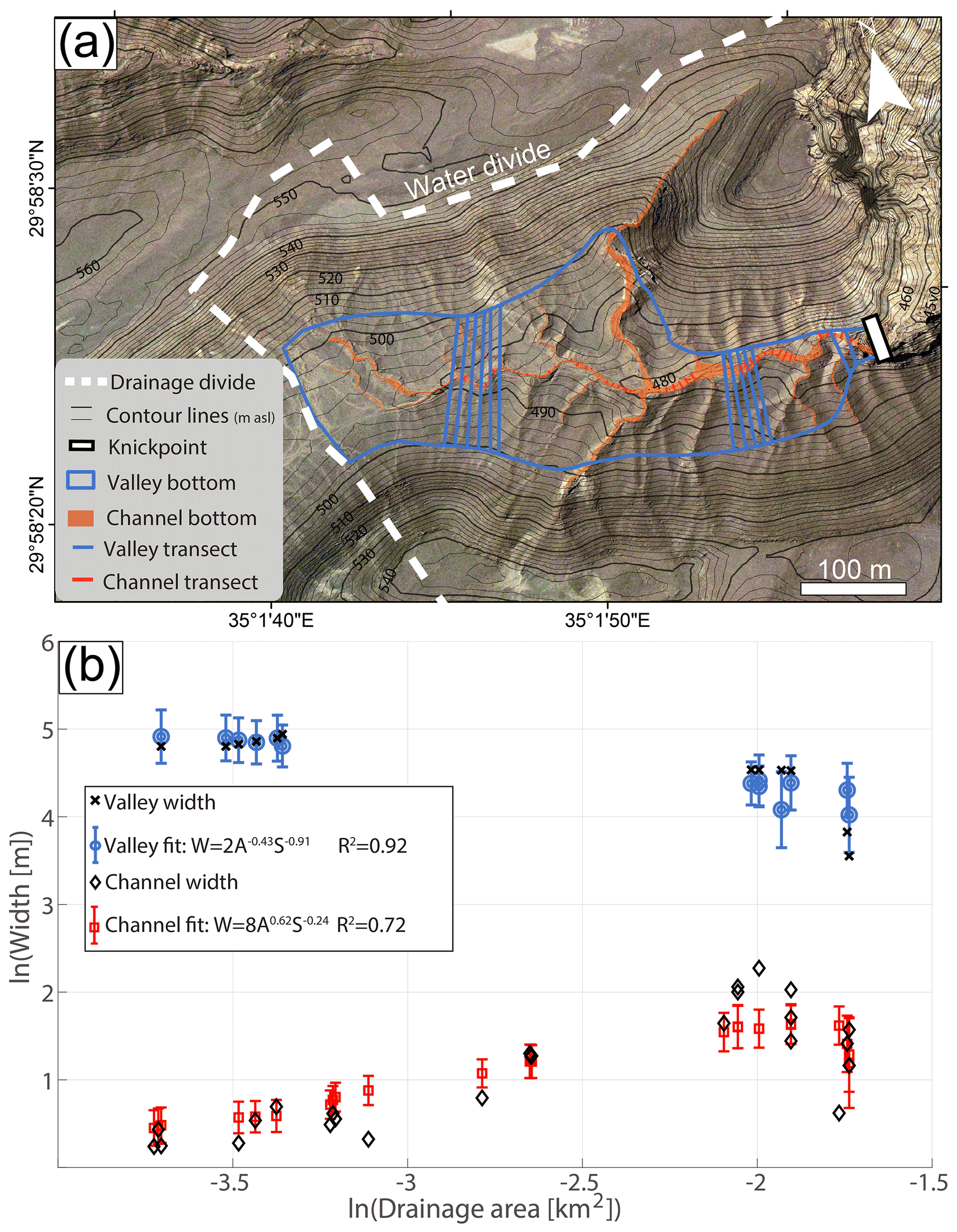
Figure 6Variations in valley and channel widths along a reversed section (valley 12 in Tables 1 and 2 as well as Fig. 1d). (a) Valley (blue) and channel (orange) polygons and width transects, sketched over a 0.5 m resolution orthophoto. The slope break between the valley bottom and the hillslope is emphasized by the density change of the 2 m contour lines (thin black lines). (b) Width–area–slope scaling of reversed valley width (data in black, fit in blue), which narrows with drainage area, contrasting with the width of the channel (data in black, fit in red) that increases downstream. This difference is expressed by the drainage area exponent, b, which is positive for the channel and negative for the valley.
Field observations show that while the reversed valley narrows downstream (i.e., eastward), the channel width increases in this direction (Fig. 6a), which is a pattern that was also observed in other reversed valley sections. In valley 12, a multivariate regression over the channel data reveals a drastically different dependency between the channel's width, drainage area, and slope compared to the valley (Fig. 6b). For the channel, the least-square multivariate regression (R2=0.72) yields a kb coefficient of 8 (10−6 m1−2b, with a 95 % coefficient interval of 3–17), a positive and high b exponent of 0.62±0.18, and a negative, statistically insignificant c exponent of . In contrast, the computed values for the valley are 2 (10−6 m with a 95 % coefficient interval of 1–6) for kb, a negative b exponent of , and a statistically significant c of .
5.1 Drainage reorganization affects the scaling of valley width–drainage area
The width–area regression results reveal that undisturbed, beheaded, and reversed valleys are characterized by a distinct range of the drainage area exponent, d, indicating the fingerprint of reorganization in the width–area scaling of valleys. In our study area, the d exponent values of the undisturbed valleys range between 0.26 and 0.54, consistent with previously published exponent values for valleys (Beeson et al., 2018; Brocard and van der Beek, 2006; Clubb et al., 2022; Langston and Temme, 2019; Schanz and Montgomery, 2016; Shepherd et al., 2013; Snyder et al., 2003; Tomkin et al., 2003). The beheaded valleys in the study area are characterized by d exponent values of 0.15–0.23. While this range partly overlaps with previously published valley width–area scaling (Beeson et al., 2018; Clubb et al., 2022; Langston and Temme, 2019; Schanz and Montgomery, 2016), it does not overlap with the d exponents of the undisturbed valleys in our study area. The low values of the d exponent of the beheaded valleys reflect a smaller increase in valley width (log (W)) per unit change in drainage area (log (A)) that is consistent with the process of beheading. During beheading, a valley loses its narrowest headwater sections, and consequently, the beheaded valley is wider at smaller drainage areas compared to undisturbed valleys (e.g., Fig. 3b). Farther downstream, as drainage area increases through contribution from non-beheaded side tributaries, the effect of beheading on drainage area decreases and the valley width–area values become similar to those of undisturbed valleys (e.g., Fig. 3a, b). Additionally, the drainage area loss reduces the discharge and sediment transport capacity near the divide and may lead to aggradation, further widening the valley bottom (Brocard and van der Beek, 2006; Langston and Tucker, 2018) in small drainage areas. These effects act to lower the slope of the log (W) [m] vs. log (A) [km2] regression line of beheaded valleys compared to undisturbed valleys (e.g., Fig. 3b).
The processes described above also increase the value of the kc coefficient of beheaded valleys compared to undisturbed valleys. However, whereas the median kc value and the overall kc range are indeed higher in beheaded valleys (Fig. 4 and Table 1), the kc difference is relatively small. The reason is likely that the kc coefficient reflects the valley width at a drainage area of 1 km2. In the study area, a 1 km2 drainage area is reached only after the beheaded section is joined by several undisturbed tributaries, which obscures the beheading influence and blurs the difference in kc coefficient among the undisturbed and beheaded valleys.
The negative value of the d exponent for the reversed valleys (between −0.18 and −1) reflects downstream valley narrowing, supporting the inferred reversal of these valley sections (Harel et al., 2019). The three southern reversed valleys (10, 11, and 12 in Tables 1 and 2 and in Fig. 1d) yield d exponents with an absolute value that is similar to that of undisturbed valley sections. This observation is consistent with the view that (i) the geometry of the antecedent valleys whose flow direction was reversed is similar to that of the undisturbed valleys (e.g., Figs. 2e, 3b, and 6), and (ii) the valley width did not drastically change following the reversal process. The d exponents in the two northern valleys (8 and 9 in Tables 1 and 2 and in Fig. 1d) have higher absolute values, reflecting strong contrast between the narrow widths close to the knickpoint (several meters) and the anomalously high widths near the wind gap (>500 m) that are likely associated with the E–W-trending strike valley that accommodates the wind gaps.
5.2 Identifying reorganization from valley width–drainage area scaling
The distinct ranges of the d exponent for the undisturbed and reorganized valley categories are consistent with the hypothesis that drainage reorganization modifies the scaling between valley width and drainage area. Based on these results, we suggest that such scaling differences could help to identify instances of drainage reorganization and point to specific categories of reorganization according to the values of inferred d exponents in these sections. Importantly, invoking d exponents to support reorganization requires comparing the suspected reorganized valley sections to undisturbed sections with similar environmental conditions because the valley widening rate could be strongly affected by local factors. Among these factors are the lithology of the valley bed and walls (Brocard and van der Beek, 2006; Langston and Temme, 2019; Langston and Tucker, 2018; Schanz and Montgomery, 2016), the climatic and glacial history of the landscape (Chen, 2021; Clubb et al., 2022; Hancock and Anderson, 2002), and geologic structures activated by tectonic forcing (Keen-Zebert et al., 2017; Whittaker et al., 2007a). Consequently, local deviations of the d exponent likely indicate reorganization only when the deviation is constrained across similar lithologic, climatic, and tectonic settings. When these conditions are met, we expect that deviations of the d exponent can serve as an effective tool for identifying reorganized drainages, regardless of the lithology and climate conditions.
5.3 Influence of channel slope on predictions of reversed valley width
Our analysis reveals that Eq. (2), which includes the local slope, yields better valley width predictions for reversed valley sections compared to Eq. (1). This is evident from the high values of adjusted R2 for the multivariate regression and the finding that in most cases, the best-fit area and slope exponents (b and c, respectively) are of the same order of magnitude.
While the relation between valley width, drainage area, and channel slope was postulated based on theoretical considerations (Brocard and van der Beek, 2006), the specific processes by which channel slope affects valley width remained vague. We suggest that in our study area, part of the correlation between the valley width and channel slope is linked to trends seen at the downstream edge of the reversed sections, above the knickpoint, where the valley narrows and the channel incises into the bedrock and steepens (e.g., valley transects in Fig. 2e, f and Fig. S9 in the Supplement). Narrowing and steepening close to the upper lip of the knickpoint are likely associated with flow acceleration above the knickpoint (Haviv et al., 2010) that forms a juvenile narrow valley (Fig. 2f). Deeper incision above the knickpoint may cause local bank collapse that erodes the remanent terraces of the paleo-valley and establishes a narrower valley that amplifies the narrowing of reversed valleys towards the knickpoints (Fig. S9 in the Supplement) and may increase the absolute value of the exponent d (Eq. 1). This process likely reflects a transient response to reorganization and the onset of valley width adjustment to the new drainage direction.
Valley 10 (Tables 1 and 2 and in Fig. 1d) is an interesting exception in this context. Here, despite a ∼ 80 m high knickpoint at the edge of the reversed section, valley narrowing above the knickpoint is not prominent, and slope increase is absent (Figs. S9 and S10 in the Supplement). The lack of incision above the knickpoint in valley 10 could imply a recent episode of knickpoint migration to its current location. Accordingly, in this case, the adjusted R2 of the multivariate regression (Eq. 2, Table 2) is only slightly higher than the standard R2 of Eq. (1) (Table 1), and the slope exponent is distinctively low (Table 2), suggesting that at this site, the inclusion of slope does not meaningfully improve the prediction of valley width.
5.4 Timescales and mechanisms of valley and channel width adjustment in reversed drainages
The comparison between the valley and channel width patterns in reversed valley 12 (Fig. 6) reveals a distinct contrast between the valley's negative b exponent, reflecting downstream valley narrowing, and the positive b exponent of the channel, reflecting downstream channel widening. We suggest that this field case demonstrates a temporal snapshot, where the channel width is adjusted to the new drainage area distribution inflicted by the drainage reversal. In contrast, the valley width is not yet adjusted to the change in drainage area (Fig. 6b), consistent with the longer timescales expected for valley adjustment relative to the channel (Hancock and Anderson, 2002; Langston and Tucker, 2018).
In the reversed category, an increase in drainage area is associated with the process of gradual divide migration within the antecedent valley (Harel et al., 2019). Field observations from valley 12 show that the latest drainage area redistribution phase is set by a small avulsion in a colluvial fan that drains the northern flank of the valley close to the wind gap (Fig. S11 in the Supplement). The main active flow path of this fan flows east toward the reversed section; however, an older path that drains westward toward the beheaded section is not completely abandoned and is likely active when the main flow path is flooded (Shelef and Goren, 2021). This setting reflects a recent episode of flow diversion and redistribution of discharge from the beheaded to the reversed valley. Therefore, the inferred positive and high exponent of the channel width–drainage area scaling (Fig. 6) demonstrates rapid channel adjustment, in line with previous studies that proposed a rapid response of channel width to environmental changes (Amos and Burbank, 2007; Attal et al., 2008; Morell et al., 2020; Snyder and Kammer, 2008; Yanites, 2018).
In deeply incised channels, where lateral erosion is minimal and hillslope erosion is enslaved to channel incision, we suggest that the time required to erode the antecedent valley bottom, t [kyr], depends on the channel's vertical incision rate, Ev [m kyr−1], the averaged hillslope angle, ∅ [m m−1], and the width of the antecedent valley, W [m]:
We apply Eq. (3) to approximate the time required for reversed valley 12 to completely erode its antecedent valley. Morphometric measurements in valley 12, based on the TanDEM-X DEM, yield a maximal valley width of 125 m near the wind gap and . Based on the ages of abandoned terraces along channels of similar drainage areas and climate (Enzel et al., 2012), we estimated Ev to range between 0.5 and 0.05 m kyr−1. With these values, Eq. (3) predicts a time range of 50–500 kyr. However, the underlying assumption of Eq. (3), that hillslopes respond instantaneously to channel incision, is not necessarily valid in arid environments where hillslope processes are slow (Ben-Asher et al., 2017; Dunne et al., 2016). The high slopes of the terrace flanks in valley 12, exceeding 0.4 in some cases, support a delayed response of the hillslope to channel incision. We therefore suggest that the predictions of Eq. (3) represent a lower bound when applied to arid environments.
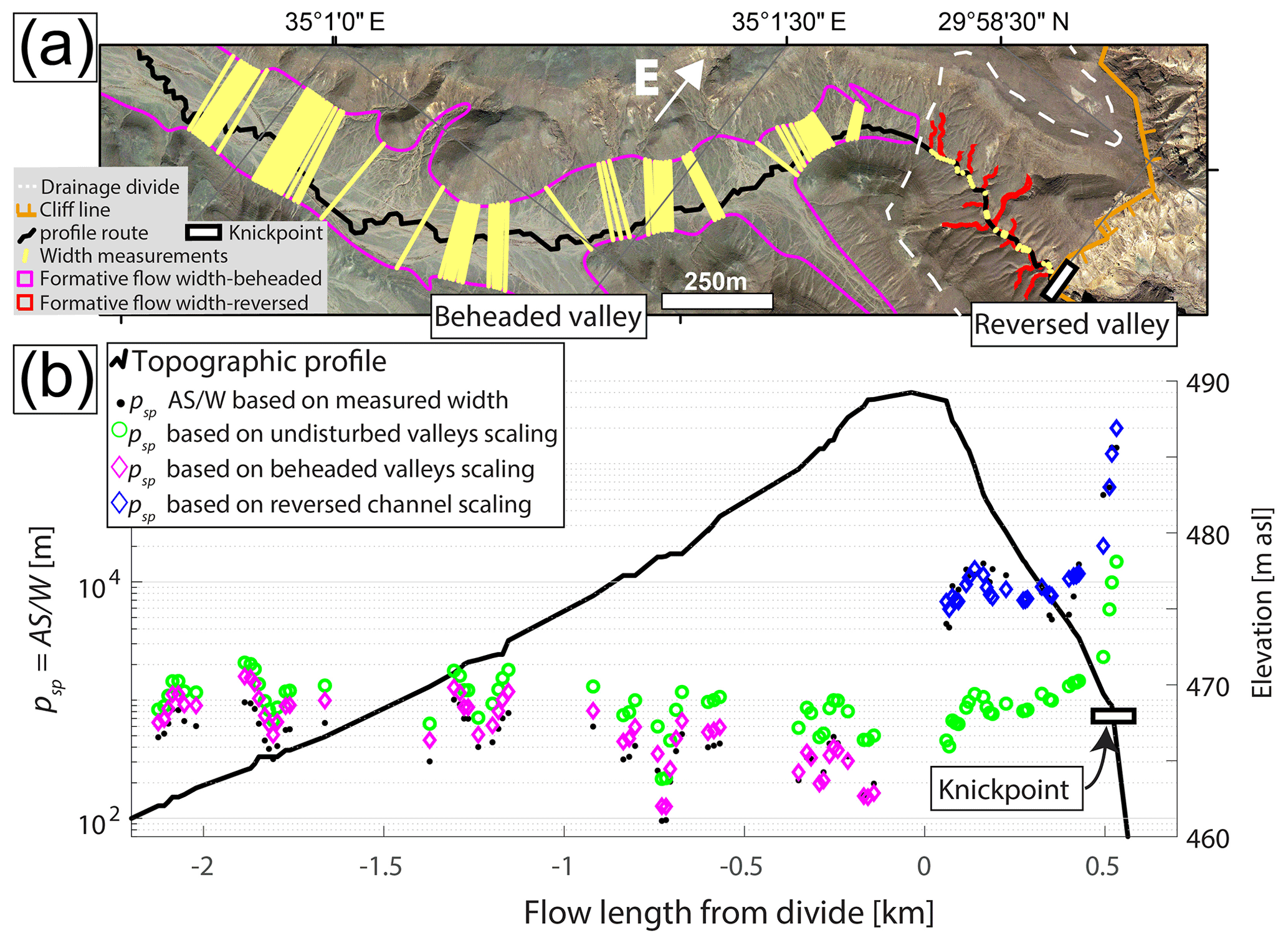
Figure 7A proxy for unit stream power () along a profile from a reversed valley (12) to a beheaded valley (6) across a wind gap. (a) An orthophoto of the reversed and beheaded valley sections that share a common wind gap. The black line marks the profile route that follows the main channels and crosses the divide. The dashed white line marks the divide, and yellow lines mark measured width transects of the formative flow width used for calculating psp. In the reversed valley, east of the wind gap, the active drainage is confined to an incised and narrow channel (Fig. 6a), whose width is used for estimating psp. West of the wind gap, in the beheaded side, the formative flow width aligns with that of the valley. (b) psp estimates based on different measurements of the formative flow width: (i) measured from DEMs (black dots), (ii) computed based on the median of the fitted predictors for undisturbed valleys in the study area (that is, without accounting for reorganization: W=100A0.47, green open circles), (iii) computed based on the scaling fitted for a beheaded valley (6 in Table 1: , pink rhombuses), and (iv) computed based on the channel scaling for a reversed channel (Fig. 6b, , blue rhombuses). The contrast between the morphological properties of the channels in the reversed and the beheaded valleys generates a distinct step change in the psp values across the wind gap, which can promote continuous wind-gap migration. The trend is not predicted by psp estimations that do not account for the unique width scaling in reorganizing valleys (green open circles).
5.5 Implications for landscape evolution
Delayed valley versus channel adjustment in response to reorganization (Fig. 6) and the diverging response of valleys of different reorganization categories (Fig. 4) have important implications for landscape evolution. We explore an example of such an implication by inspecting the influence of channel and valley width adjustment on a proxy for the unit stream power ( – W m−1; ρ: density, g: gravitational acceleration, Q: discharge), which is commonly used for evaluating fluvial erosion rate (e.g., Harbor, 1998; Magilligan et al., 2015). Given that ρg can be treated as a constant and that Q is typically proportional to drainage area, the unit stream power is proportional to [m] (Whittaker et al., 2007a). Using the width of the formative flows for W, psp is calculated to explore changes in unit stream power across the wind gap between reversed valley 12 and beheaded valley 6 (Fig. 7a).
Field observations demonstrate that the formative flows of reversed valley 12 are currently confined to the narrow, actively incising channel (Figs. 2e, 6, and 7a), resulting in comparably high values of psp. In contrast, across the wind gap, in beheaded valley 6, the psp values are an order of magnitude lower because here the wide valley defines the width of the formative flows, which fully occupy the flat alluvial valley bed (Figs. 2d and 7a). This difference results in a substantial step change in the psp values across the wind gap (Fig.7b, black dots), suggesting that the wind gap is unstable and likely to migrate in the direction of beheaded valley 6.
Harel et al. (2019) proposed that in this study area, valley reversal initiates and extends by gradual wind-gap migration along an antecedent valley. Wind-gap migration increases the drainage area along the reversed segment and, according to the response documented in valley 12, contributes to the incision of a narrow channel within the wider antecedent valley. Across the wind gap, drainage area loss hinders incision on the beheaded side, and the formative flow remains exceptionally wide. These differences in valley response and formative flow width contribute to the psp step change across the wind gap and, consequently, to erosion rate differences that promote further wind-gap migration toward the beheaded valley. This “width feedback” adds to the drainage area feedback (Willett et al., 2014) in facilitating ongoing wind-gap migration, extending the reversed segment and shrinking the beheaded segment.
Importantly, the psp values of the beheaded valley (valley 6) represent a conservative estimation. First, the flatness of the beheaded valley hints that transport-limited conditions and aggradation may dominate changes in valley bed elevation rather than vertical erosion (Brocard and van der Beek, 2006; Finnegan and Balco, 2013). Second, the limited sediment transport capacity and associated sediment aggradation over the beheaded valley bed could contribute to a relatively permeable valley fill that increases infiltration and decreases the effective discharge per drainage area.
The step change in psp values across the wind gap emphasizes the importance of accurate channel and valley width estimates when exploring the evolution of landscapes undergoing drainage reorganization. More specifically, when the width is approximated based on simple width–drainage area scaling, without accounting for the influence of reorganization (e.g., green open circles in Fig. 7b), the psp values meaningfully deviate from the measured values (green open circles relative to black dots in Fig. 7b), the aforementioned step change in psp is not recognized (Fig. 7b, green open circles), and the wind gap will be wrongly assumed as stable (Fig. 7b). In contrast, psp estimations based on scaling that account for reorganization are consistent with the measured psp values (blue and pink rhombuses relative to black dots in Fig. 7b) and emphasize the erosion rate difference between the reversed and the beheaded valley sections that reflects the instability of the wind gap between them.
Analysis of undisturbed and reorganized valley sections in the Negev desert reveals that the scaling between valley width and drainage area (Eq. 1) is affected by drainage reorganization. Each reorganization category is associated with a distinct range of drainage area exponent values, d, that relate the valley width to the drainage area. In the undisturbed valleys, the range of d exponent values is overall consistent with values reported in previous studies (e.g., Beeson et al., 2018; Clubb et al., 2022; Langston and Temme, 2019; Schanz and Montgomery, 2016). The d exponent values of the beheaded valleys are positive and smaller than in undisturbed valleys. In the reversed valleys, the d exponent values are negative, reflecting valley narrowing with increasing drainage area. We propose that these deviations could benefit future studies that aim to identify and categorize drainage reorganization by comparing the width–area scaling of suspected reorganized drainages to those of undisturbed valleys with similar lithologic, climatic, and tectonic conditions.
Most reversed valleys exhibit poor covariance between slope and drainage area. Therefore, in this category, the valley width scaling was also inspected through Eq. (2), which incorporates both the slope and drainage area as predictors of valley width. This multivariate analysis results in higher adjusted R2 values than those produced by Eq. (1) and resulted in negative exponents for both area and slope (b and c, respectively) with the same order of magnitude, indicating that they are both significant for the valley width prediction in the reversed category.
In the reversed valleys, differences in width–area–slope scaling also occur between a channel and its hosting valley. In a reversed valley section analyzed in detail, we found that the channel width is best fitted by a positive area exponent b, whereas the exponent for the valley width is negative, reflecting a faster adjustment of channel width to the post-reorganization drainage area distribution relative to the adjustment of valley width. This case study of a reversed valley section that shares a common wind gap with a beheaded valley illustrates the significance of the contrasting timescales of channel and valley width adjustment for landscape evolution. The difference between the narrow active channel in the reversed section and the wide formative flows that occupy the entire width of the beheaded valley across the wind gap results in a step change in the unit stream power across the wind gap, used here as a proxy for fluvial erosion rate. Consequently, the step change in unit stream power promotes divide migration and is a part of a divide migration feedback: erosion rate gradients across the wind gap push the wind gap toward the beheaded valley, which has a smaller unit stream power due to its wider channel and lower slope. Wind-gap migration induces rapid channel width adjustment on the extending reversed side, while on the beheaded side, adjustment is delayed, sustaining the gradient in unit stream power. This feedback suggests that the differing response of channel and valley width in different reorganization categories could maintain ongoing divide migration and may add to the slope and area feedbacks that were previously invoked as drivers of divide migration (Plant et al., 2014; Shelef and Goren, 2021; Willett et al., 2014). This width feedback could be easily overlooked if the channel width is parameterized based on a standard scaling relation, which is commonly assumed in large-scale landscape evolution models (e.g., Goren et al., 2014; Lague et al., 2014; Shobe et al., 2017; Yanites et al., 2013).
Insights from this study point to several avenues for future research. For example, what are the constraints on the timescales over which the deviation in scaling persists? How do they vary with climate and lithology? Could the values of area exponents d or b quantify the temporal state of channel and valley adjustment? And what is the relation of the dynamics and rates of divide migration to the width adjustment of valleys and channels?
The ArcGIS model for the width measurements is fully described in the Supplement and can be downloaded at https://doi.org/10.5281/zenodo.7007928 (Harel, 2022a).
The study is based on the copyrighted 12 m TanDEM-X that is available for scientific use with a service fee charge via the following link: https://tandemx-science.dlr.de/cgi-bin/wcm.pl?page=TDM-Proposal-Submission-Procedure (Wessel, 2016). The data on width, slope, and drainage area of the analyzed sections, as well as kml shapefiles of the valley bottom polygons before and after manual editing and of the width measurements, are available at https://doi.org/10.5281/zenodo.6970603 (Harel, 2022b).
The supplement related to this article is available online at: https://doi.org/10.5194/esurf-10-875-2022-supplement.
LG and ES conceptualized the project. EH developed the software for extracting valley and channel width and performing the regression, with input from LG and ES. EH analyzed the data, generated the figures, and wrote the initial draft. LG, ES, and OC reviewed and edited the paper and supervised the research. HG introduced us to the field area and contributed to the ideas presented in this paper.
The contact author has declared that none of the authors has any competing interests.
Publisher's note: Copernicus Publications remains neutral with regard to jurisdictional claims in published maps and institutional affiliations.
We thank the German Aerospace Center (DLR) for providing the 0.4 arcsec TanDEM-X. We also acknowledge our field assistants, Eitan Meidad, Gad Reifman, Haran Henig, Omri Porat, Tom Kaner, and Yaakov Prois. Elhanan Harel thanks the Nehemia Levtzion scholarship for its support. We thank Charles Shobe, George Hilley, and the anonymous reviewer for their constructive comments that significantly improved this paper. George Hilley suggested Eq. (3) for estimating the time required to eliminate the antecedent valley width.
This research has been supported by the United States–Israel Binational Science Foundation (grant nos. 1946253 (NSF) and 2019656 (BSF)).
This paper was edited by Fiona Clubb and reviewed by George Hilley, Charles Shobe, and one anonymous referee.
Allen, G. H., Barnes, J. B., Pavelsky, T. M., and Kirby, E.: Lithologic and tectonic controls on bedrock channel form at the northwest Himalayan front, J. Geophys. Res. Earth Surf., 118, 1806–1825, https://doi.org/10.1002/jgrf.20113, 2013.
Amit, R., Enzel, Y., and Sharon, D.: Permanent Quaternary hyperaridity in the Negev, Israel, resulting from regional tectonics blocking Mediterranean frontal systems, Geology, 34, 509–512, https://doi.org/10.1130/G22354.1, 2006.
Amit, R., Simhai, O., Ayalon, A., Enzel, Y., Matmon, A., Crouvi, O., Porat, N., and McDonald, E.: Transition from arid to hyper-arid environment in the southern Levant deserts as recorded by early Pleistocene cummulic Aridisols, Quat. Sci. Rev., 30, 312–323, https://doi.org/10.1016/j.quascirev.2010.11.007, 2011.
Amos, C. B. and Burbank, D. W.: Channel width response to differential uplift, J. Geophys. Res. Earth Surf., 112, 1–11, https://doi.org/10.1029/2006JF000672, 2007.
Attal, M., Tucker, G. E., Whittaker, A. C., Cowie, P. A., and Roberts, G. P.: Modelling fluvial incision and transient landscape evolution: Influence of dynamic Channel adjustment, J. Geophys. Res. Earth Surf., 113, 1–16, https://doi.org/10.1029/2007JF000893, 2008.
Avni, Y., Bartov, Y., Garfunkel, Z., and Ginat, H.: Evolution of the Paran drainage basin and its relation to the Plio-Pleistocene history of the Arava Rift western margin, Israel., Isr. J. Earth Sci., 49, 215–238, https://doi.org/10.1560/W8WL-JU3Y-KM7W-8LX4, 2000.
Avni, Y., Segev, A., and Ginat, H.: Oligocene regional denudation of the northern Afar dome: Pre- and syn-breakup stages of the Afro-Arabian plate, Bull. Geol. Soc. Am., 124, 1871–1897, https://doi.org/10.1130/B30634.1, 2012.
Beeson, H. W., Flitcroft, R. L., Fonstad, M. A., and Roering, J. J.: Deep-Seated Landslides Drive Variability in Valley Width and Increase Connectivity of Salmon Habitat in the Oregon Coast Range, JAWRA J. Am. Water Resour. Assoc., 54, 1325–1340, 2018.
Ben-Asher, M., Haviv, I., Roering, J. J., and Crouvi, O.: The influence of climate and microclimate (aspect) on soil creep efficiency: Cinder cone morphology and evolution along the eastern Mediterranean Golan Heights, Earth Surf. Process. Landforms, 42, 2649–2662, https://doi.org/10.1002/esp.4214, 2017.
Bertrand, M. and Liébault, F.: Active channel width as a proxy of sediment supply from mining sites in New Caledonia, Earth Surf. Process. Landforms, 44, 67–76, https://doi.org/10.1002/esp.4478, 2019.
Bishop, P.: Drainage rearrangement by river capture, beheading and diversion, Prog. Phys. Geogr., 19, 449–473, https://doi.org/10.1177/030913339501900402, 1995.
Bitan, A. and Rubin, S.: Climatic atlas of Israel for physical and environmental planning and design, Minist. Transp. Jerusalem, 1991.
Brocard, G. Y. and van der Beek, P. A.: Influence of incision rate, rock strength, and bedload supply on bedrock river gradients and valley-flat widths: Field-based evidence and calibrations from western Alpine rivers (southeast France), Spec. Pap. Geol. Soc. Am., 398, 101–126, 2006.
Brussock, P. P., Brown, A. V., and Dixon, J. C.: Channel Form And Stream Ecosystem Models, JAWRA J. Am. Water Resour. Assoc., 21, 859–866, https://doi.org/10.1111/j.1752-1688.1985.tb00180.x, 1985.
Chen, A.: Climatic controls on drainage basin hydrology and topographic evolution, University of Bristol, https://research-information.bris.ac.uk/ws/portalfiles/portal/280935962/Final_Copy_2021_07_01_Chen_S_A_PhD.pdf (last access: 4 September 2022), 2021.
Clubb, F. J., Mudd, S. M., Milodowski, D. T., Valters, D. A., Slater, L. J., Hurst, M. D., and Limaye, A. B.: Geomorphometric delineation of floodplains and terraces from objectively defined topographic thresholds, Earth Surf. Dynam., 5, 369–385, https://doi.org/10.5194/esurf-5-369-2017, 2017.
Clubb, F. J., Weir, E. F., and Mudd, S. M.: Continuous measurements of valley floor width in mountainous landscapes, Earth Surf. Dynam., 10, 437–456, https://doi.org/10.5194/esurf-10-437-2022, 2022.
Davis, W. M.: A river-pirate, Science, 13, 108–109, 1889.
Dunne, T. and Leopold, L. B.: Water in environmental planning, Macmillan, 1978.
Dunne, T., Malmon, D. V., and Dunne, K. B. J.: Limits on the morphogenetic role of rain splash transport in hillslope evolution, J. Geophys. Res. Earth Surf., 121, 609–622, https://doi.org/10.1002/2015JF003737, 2016.
Dury, G. H.: Principles of underfit streams, US Government Printing Office, 1964.
Enzel, Y., Amit, R., Grodek, T., Ayalon, A., Lekach, J., Porat, N., Bierman, P., Blum, J. D., and Erel, Y.: Late Quaternary weathering, erosion, and deposition in Nahal Yael, Israel: An “impact of climatic change on an arid watershed”?, Bulletin, 124, 705–722, 2012.
Fan, N., Chu, Z., Jiang, L., Hassan, M. A., Lamb, M. P., and Liu, X.: Abrupt drainage basin reorganization following a Pleistocene river capture, Nat. Commun., 9, 1–6, 2018.
Faustini, J. M., Kaufmann, P. R., and Herlihy, A. T.: Downstream variation in bankfull width of wadeable streams across the conterminous United States, Geomorphology, 108, 292–311, https://doi.org/10.1016/J.GEOMORPH.2009.02.005, 2009.
Finnegan, N. J. and Balco, G.: Sediment supply, base level, braiding, and bedrock river terrace formation: Arroyo Seco, California, USA, Bull. Geol. Soc. Am., 125, 1114–1124, https://doi.org/10.1130/B30727.1, 2013.
Finnegan, N. J., Roe, G., Montgomery, D. R., and Hallet, B.: Controls on the channel width of rivers: Implications for modeling fluvial incision of bedrock, Geology, 33, 229–232, https://doi.org/10.1130/G21171.1, 2005.
Fisher, G. B., Bookhagen, B., and Amos, C. B.: Channel planform geometry and slopes from freely available high-spatial resolution imagery and DEM fusion: Implications for channel width scalings, erosion proxies, and fluvial signatures in tectonically active landscapes, Geomorphology, 194, 46–56, https://doi.org/10.1016/j.geomorph.2013.04.011, 2013.
Flint, J. J.: Stream gradient as a function of order, magnitude, and discharge, Water Resour. Res., 10, 969–973, https://doi.org/10.1029/WR010i005p00969, 1974.
Fryirs, K. A., Brierley, G. J., Wheaton, J. M., Bizzi, S., and Williams, R.: To plug-in or not to plug-in? Geomorphic analysis of rivers using the River Styles Framework in an era of big data acquisition and automation, WIREs Water, 6, e1372, https://doi.org/10.1002/wat2.1372, 2019.
Garfunkel, Z.: Internal structure of the Dead Sea leaky transform (rift) in relation to plate kinematics, Tectonophysics, 80, 81–108, 1981.
Garfunkel, Z.: Lateral Motion and Deformation Along the Dead Sea Transform BT – Dead Sea Transform Fault System: Reviews, edited by: Garfunkel, Z., Ben-Avraham, Z., and Kagan, E., Springer Netherlands, Dordrecht, 109–150, https://doi.org/10.1007/978-94-017-8872-4_5, 2014.
Garfunkel, Z. and Horowitz, A.: The upper Tertiary and Quaternary morphology of the Negev, Israel, Isr. J. Earth Sci, 15, 101–117, 1966.
Giaconia, F., Booth-Rea, G., Martínez-Martínez, J. M., Azañón, J. M., Pérez-Peña, J. V., Pérez-Romero, J., and Villegas, I.: Geomorphic evidence of active tectonics in the Sierra Alhamilla (eastern Betics, SE Spain), Geomorphology, 145–146, 90–106, https://doi.org/10.1016/j.geomorph.2011.12.043, 2012.
Gibling, M. R.: Width and Thickness of Fluvial Channel Bodies and Valley Fills in the Geological Record: A Literature Compilation and Classification, J. Sediment. Res., 76, 731–770, https://doi.org/10.2110/jsr.2006.060, 2006.
Gilbert, J. T., Macfarlane, W. W., and Wheaton, J. M.: The Valley Bottom Extraction Tool (V-BET): A GIS tool for delineating valley bottoms across entire drainage networks, Comput. Geosci., 97, 1–14, https://doi.org/10.1016/j.cageo.2016.07.014, 2016.
Ginat, H.: The geology and geomorphology of Yotvata Region, Isr. Geol. Surv. Rep., GSI/8/91, https://www.gov.il/BlobFolder/reports/reports-1991/he/report_1991_Ginat-H-Geology-Geomorphology-Yotvata-Region-1991-GSI-08-91-MSc-Thesis-HUJI.pdf (last access: 4 September 2022), 1991 (in Hebrew with English abstract).
Ginat, H.: Paleogeography and the landscape evolution of the Nahal Hiyyon and Nahal Zihor basins (sedimentology, climatic and tectonic aspects), PhD Diss., Israel Geological Survey Report, GSI/19/97, 206, https://www.gov.il/BlobFolder/reports/reports-1997/he/report_1997_Ginat-H-Paleogeography-Landscape-Evolution-Nahal-Hiyyon-Nahal-Zihor-GSI-19-1997-PhD-Thesis.pdf (last access: 4 September 2022), 1997 (in Hebrew with English abstract).
Ginat, H., Zilberman, E., and Avni, Y.: Tectonic and paleogeographic significance of the Edom River, a Pliocene stream that crossed the Dead Sea Rift valley, Isr. J. Earth Sci., 49, 159–177, https://doi.org/10.1560/N2P9-YBJ0-Q44Y-GWYN, 2000.
Ginat, H., Zilberman, E., and Amit, R.: Red sedimentary units as indicators of Early Pleistocene tectonic activity in the southern Negev desert, Israel, Geomorphology, 45, 127–146, https://doi.org/10.1016/S0169-555X(01)00193-3, 2002.
Ginat, H., Opitz, S., Ababneh, L., Faershtein, G., Lazar, M., Porat, N., and Mischke, S.: Pliocene-Pleistocene waterbodies and associated deposits in southern Israel and southern Jordan, J. Arid Environ., 148, 14–33, https://doi.org/10.1016/j.jaridenv.2017.09.007, 2018.
Golly, A. and Turowski, J. M.: Deriving principal channel metrics from bank and long-profile geometry with the R package cmgo, Earth Surf. Dynam., 5, 557–570, https://doi.org/10.5194/esurf-5-557-2017, 2017.
Goren, L., Willett, S. D., Herman, F., and Braun, J.: Coupled numerical-analytical approach to landscape evolution modeling, Earth Surf. Process. Landforms, 39, 522–545, https://doi.org/10.1002/esp.3514, 2014.
Guralnik, B., Matmon, A., Avni, Y., and Fink, D.: 10Be exposure ages of ancient desert pavements reveal Quaternary evolution of the Dead Sea drainage basin and rift margin tilting, Earth Planet. Sci. Lett., 290, 132–141, https://doi.org/10.1016/j.epsl.2009.12.012, 2010.
Hancock, G. S. and Anderson, R. S.: Numerical modeling of fluvial strath-terrace formation in response to oscillating climate, GSA Bull., 114, 1131–1142, https://doi.org/10.1130/0016-7606(2002)114<1131:NMOFST>2.0.CO;2, 2002.
Harbor, D. J.: Dynamic equilibrium between an active uplift and the Sevier River, Utah, J. Geol., 106, 181–194, 1998.
Harel, E.: ArcGIS model for optimal valley width measurement, Zenodo [code], https://doi.org/10.5281/zenodo.7007928, 2022a.
Harel, E.: Width area slope data, valley bottom polygons and width measurements, Zenodo [data set], https://doi.org/10.5281/zenodo.6970603, 2022b.
Harel, E., Goren, L., Shelef, E., and Ginat, H.: Drainage reversal toward cliffs induced by lateral lithologic differences, Geology, 47, 928–932, https://doi.org/10.1130/G46353.1, 2019.
Haviv, I., Enzel, Y., Whipple, K. X., Zilberman, E., Matmon, A., Stone, J., and Fifield, K. L.: Evolution of vertical knickpoints (waterfalls) with resistant caprock: Insights from numerical modeling, J. Geophys. Res.-Earth, 115, F03028, https://doi.org/10.1029/2008JF001187, 2010.
Hilley, G. E., Baden, C. W., Dobbs, S. C., Plante, Z., Sare, R., and Steelquist, A. T.: A Curvature-Based Method for Measuring Valley Width Applied to Glacial and Fluvial Landscapes, J. Geophys. Res. Earth Surf., 125, e2020JF005605, https://doi.org/10.1029/2020JF005605, 2020.
Jones, J. C.: Historical channel change caused by a century of flow alteration on Sixth Water Creek and Diamond Fork River, UT, Utah State University, https://doi.org/10.26076/8475-a88e, 2018.
Keen-Zebert, A., Hudson, M. R., Shepherd, S. L., and Thaler, E. A.: The effect of lithology on valley width, terrace distribution, and bedload provenance in a tectonically stable catchment with flat-lying stratigraphy, Earth Surf. Process. Landforms, 42, 1573–1587, https://doi.org/10.1002/esp.4116, 2017.
Kirby, E. and Ouimet, W.: Tectonic geomorphology along the eastern margin of Tibet: Insights into the pattern and processes of active deformation adjacent to the Sichuan Basin, Geol. Soc. Spec. Publ., 353, 165–188, https://doi.org/10.1144/SP353.9, 2011.
Lague, D.: The stream power river incision model: Evidence, theory and beyond, Earth Surf. Process. Landforms, 39, 38–61, https://doi.org/10.1002/esp.3462, 2014.
Langston, A. L. and Temme, A. J. A. M.: Impacts of Lithologically Controlled Mechanisms on Downstream Bedrock Valley Widening, Geophys. Res. Lett., 46, 12056–12064, 2019.
Langston, A. L. and Tucker, G. E.: Developing and exploring a theory for the lateral erosion of bedrock channels for use in landscape evolution models, Earth Surf. Dynam., 6, 1–27, https://doi.org/10.5194/esurf-6-1-2018, 2018.
Lavé, J. and Avouac, J.-P.: Fluvial incision and tectonic uplift across the Himalayas of central Nepal, J. Geophys. Res. Solid Earth, 106, 26561–26591, 2001.
Leopold, L. B. and Maddock, T. J.: The Hydraulic Geomtry of Stream Channels and Some Physiographic Implications, Geol. Surv. Prof. Pap. 252, 57, 1953.
Li, T., Fuller, T. K., Sklar, L. S., Gran, K. B., and Venditti, J. G.: A Mechanistic Model for Lateral Erosion of Bedrock Channel Banks by Bedload Particle Impacts, J. Geophys. Res.-Earth, 125, e2019JF005509, https://doi.org/10.1029/2019JF005509, 2020.
Lóczy, D., Kis, É., and Schweitzer, F.: Local flood hazards assessed from channel morphometry along the Tisza River in Hungary, Geomorphology, 113, 200–209, https://doi.org/10.1016/j.geomorph.2009.03.013, 2009.
Looper, J. P., Vieux, B. E., and Moreno, M. A.: Assessing the impacts of precipitation bias on distributed hydrologic model calibration and prediction accuracy, J. Hydrol., 418, 110–122, 2012.
Magilligan, F. J., Buraas, E. M., and Renshaw, C. E.: The efficacy of stream power and flow duration on geomorphic responses to catastrophic flooding, Geomorphology, 228, 175–188, 2015.
Manning, R., Griffith, J. P., Pigot, T. F., and Vernon-Harcourt, L. F.: On the flow of water in open channels and pipes, 1890.
Marcotte, A. L., Neudorf, C. M., and Langston, A. L.: Lateral bedrock erosion and valley formation in a heterogeneously layered landscape, Northeast Kansas, Earth Surf. Proc. Land., 46, 2248–2263, https://doi.org/10.1002/esp.5172, 2021.
Mashael Al, S.: Assessment of Flood Hazard of Jeddah Area 2009, Saudi Arabia, J. Water Resour. Prot., 2, 839–847, https://doi.org/10.4236/jwarp.2010.29099, 2010.
May, C., Roering, J., Eaton, L. S., and Burnett, K. M.: Controls on valley width in mountainous landscapes: The role of landsliding and implications for salmonid habitat, Geology, 41, 503–506, https://doi.org/10.1130/G33979.1, 2013.
Menier, D., Mathew, M., Pubellier, M., Sapin, F., Delcaillau, B., Siddiqui, N., Ramkumar, M., and Santosh, M.: Landscape response to progressive tectonic and climatic forcing in NW Borneo: Implications for geological and geomorphic controls on flood hazard, Scientific Reports, 7, 457, https://doi.org/10.1038/s41598-017-00620-y, 2017.
Monegaglia, F., Zolezzi, G., Güneralp, I., Henshaw, A. J., and Tubino, M.: Environmental Modelling & Software Automated extraction of meandering river morphodynamics from multitemporal remotely sensed data, Environ. Model. Softw., 105, 171–186, https://doi.org/10.1016/j.envsoft.2018.03.028, 2018.
Montgomery, D. R.: Observations on the role of lithology in strath terrace formation and bedrock channel width, Am. J. Sci., 304, 454–476, https://doi.org/10.2475/ajs.304.5.454, 2004.
Montgomery, D. R. and Gran, K. B.: Downstream variations in the width of bedrock channels, Water Resour. Res., 37, 1841–1846, https://doi.org/10.1029/2000WR900393, 2001.
Morell, K. D., Styron, R., Stirling, M., Griffin, J., Archuleta, R., and Onur, T.: Seismic Hazard Analyses From Geologic and Geomorphic Data: Current and Future Challenges, Tectonics, 39, e2018TC005365, https://doi.org/10.1029/2018TC005365, 2020.
O'Callaghan, J. F. and Mark, D. M.: The extraction of drainage networks from digital elevation data, Comput. Vision, Graph. Image Process., 27, 247, https://doi.org/10.1016/S0734-189X(84)80047-X, 1984.
Pechlivanidou, S., Cowie, P. A., Duclaux, G., Nixon, C. W., Gawthorpe, R. L., and Salles, T.: Tipping the balance: Shifts in sediment production in an active rift setting, Geology, 47, 259–262, https://doi.org/10.1130/G45589.1, 2019.
Plant, N. G., Flocks, J., Stockdon, H. F., Long, J. W., Guy, K., Thompson, D. M., Cormier, J. M., Smith, C. G., and Miselis, J. L.: Predictions of barrier island berm evolution in a time-varying storm climatology, J. Geophys. Res.-Earth Surf., 119, 300–316, https://doi.org/10.1002/2013JF002871, 2014.
Prince, P. S., Spotila, J. A., and Henika, W. S.: Stream capture as driver of transient landscape evolution in a tectonically quiescent setting, Geology, 39, 823–826, https://doi.org/10.1130/G32008.1, 2011.
Roux, C., Alber, A., Bertrand, M., Vaudor, L., and Piégay, H.: “FluvialCorridor”: A new ArcGIS toolbox package for multiscale riverscape exploration, Geomorphology, 242, 29–37, https://doi.org/10.1016/j.geomorph.2014.04.018, 2015.
Rowland, J. C., Shelef, E., Pope, P. A., Muss, J., Gangodagamage, C., Brumby, S. P., and Wilson, C. J.: Remote Sensing of Environment A morphology independent methodology for quantifying planview river change and characteristics from remotely sensed imagery, Remote Sens. Environ., 184, 212–228, https://doi.org/10.1016/j.rse.2016.07.005, 2016.
Sampson, C. C., Smith, A. M., Bates, P. D., Neal, J. C., Alfieri, L., and Freer, J. E.: A high-resolution global flood hazard model, Water Resour. Res., 51, 7358–7381, https://doi.org/10.1002/2015WR016954, 2015.
Schanz, S. A. and Montgomery, D. R.: Geomorphology Lithologic controls on valley width and strath terrace formation, Geomorphology, 258, 58–68, https://doi.org/10.1016/j.geomorph.2016.01.015, 2016.
Schumm, S. A. and Ethridge, F. G.: Origin, evolution and morphology of fluvial valleys, Incised-Valley Systems: Origin and Sedimentary Sequences, edited by: Robert, D. W., Boyd, R., and Zaitlin, B. A., SPEM (Society for Sedimentary Geology), https://doi.org/10.2110/pec.94.12.0011, 1994.
Sechu, G. L., Nilsson, B., Iversen, B. V, Greve, M. B., Børgesen, C. D., and Greve, M. H.: A stepwise gis approach for the delineation of river valley bottom within drainage basins using a cost distance accumulation analysis, Water (Switzerland), 13, 827, https://doi.org/10.3390/w13060827, 2021.
Shelef, E. and Goren, L.: The rate and extent of wind-gap migration regulated by tributary confluences and avulsions, Earth Surf. Dynam., 9, 687–700, https://doi.org/10.5194/esurf-9-687-2021, 2021.
Shepherd, S. L., Dixon, J. C., Davis, R. K., Shepherd, S. L., Dixon, J. C., Davis, R. K., Ozark, A., Shepherd, S. L., Dixon, J. C., and Davis, R. K.: Are Ozark Streams Underfit? Using Gis to Re- Examine Dury ' s Theory of Underfit Streams Re-Examine Dury'S Theory Of Underfit Streams, Phys. Geogr., 32, 179–194, https://doi.org/10.2747/0272-3646.32.2.179, 2013.
Shobe, C. M., Tucker, G. E., and Barnhart, K. R.: The SPACE 1.0 model: a Landlab component for 2-D calculation of sediment transport, bedrock erosion, and landscape evolution, Geosci. Model Dev., 10, 4577–4604, https://doi.org/10.5194/gmd-10-4577-2017, 2017.
Snyder, N. P. and Kammer, L. L.: Dynamic adjustments in channel width in response to a forced diversion: Gower Gulch, Death Valley National Park, California, Geology, 36, 187–190, https://doi.org/10.1130/G24217A.1, 2008.
Snyder, N. P., Whipple, K. X., Tucker, G. E., and Merritts, D. J.: Channel response to tectonic forcing: Field analysis of stream morphology and hydrology in the Mendocino triple junction region, northern California, Geomorphology, 53, 97–127, https://doi.org/10.1016/S0169-555X(02)00349-5, 2003.
Spotila, J. A., Moskey, K. A., and Prince, P. S.: Geomorphology Geologic controls on bedrock channel width in large, slowly-eroding catchments: Case study of the New River in eastern North America, Geomorphology, 230, 51–63, https://doi.org/10.1016/j.geomorph.2014.11.004, 2015.
Sweeney, B. W., Bott, T. L., Jackson, J. K., Kaplan, L. A., Newbold, J. D., Standley, L. J., Hession, W. C., and Horwitz, R. J.: Riparian deforestation, stream narrowing, and loss of stream ecosystem services, Proc. Natl. Acad. Sci. USA, 101, 14132–14137, https://doi.org/10.1073/pnas.0405895101, 2004.
Tomkin, J. H., Brandon, M. T., Pazzaglia, F. J., Barbour, J. R., and Willett, S. D.: Quantitative testing of bedrock incision models for the Clearwater River, NW Washington State, J. Geophys. Res. Solid Earth, 108, 2308, https://doi.org/10.1029/2001jb000862, 2003.
Turowski, J. M.: Alluvial cover controlling the width, slope and sinuosity of bedrock channels, Earth Surf. Dynam., 6, 29–48, https://doi.org/10.5194/esurf-6-29-2018, 2018.
Turowski, J. M.: Mass balance, grade, and adjustment timescales in bedrock channels, Earth Surf. Dynam., 8, 103–122, https://doi.org/10.5194/esurf-8-103-2020, 2020.
Vaks, A., Woodhead, J., Bar-Matthews, M., Ayalon, A., Cliff, R. A., Zilberman, T., Matthews, A., and Frumkin, A.: Pliocene–Pleistocene climate of the northern margin of Saharan–Arabian Desert recorded in speleothems from the Negev Desert, Israel, Earth Planet. Sci. Lett., 368, 88–100, https://doi.org/10.1016/j.epsl.2013.02.027, 2013.
Wessel, B.: TanDEM-X Ground Segment – DEM Products Specification Document, EOC, DLR, Oberpfaffenhofen, Germany, Public Document TD-GS-PS-0021, Issue 3.1, https://tandemx-science.dlr.de/ (last access: 4 September 2022), 2016 (data available at: https://tandemx-science.dlr.de/cgi-bin/wcm.pl?page=TDM-Proposal-Submission-Procedure, 4 September 2022).
Whipple, K. X., DiBiase, R. A., and Crosby, B. T.: Bedrock Rivers, in Treatise on Geomorphology, 9, Elsevier Ltd., 550–573, https://doi.org/10.1016/B978-0-12-374739-6.00254-2, 2013.
Whipple, K. X., Forte, A. M., DiBiase, R. A., Gasparini, N. M., and Ouimet, W. B.: Timescales of landscape response to divide migration and drainage capture: Implications for the role of divide mobility in landscape evolution, J. Geophys. Res. Earth Surf., 122, 248–273, 2017.
Whitbread, K., Jansen, J., Bishop, P., and Attal, M.: Substrate, sediment, and slope controls on bedrock channel geometry in postglacial streams, J. Geophys. Res. Earth Surf., 120, 779–798, https://doi.org/10.1002/2014JF003295, 2015.
Whittaker, A. C., Cowie, P. A., Attal, M., Tucker, G. E., and Roberts, G. P.: Bedrock channel adjustment to tectonic forcing: Implications for predicting river incision rates, Geology, 35, 103–106, https://doi.org/10.1130/G23106A.1, 2007a.
Whittaker, A. C., Cowie, P. A., Attal, M., Tucker, G. E., and Roberts, G. P.: Contrasting transient and steady-state rivers crossing active normal faults: New field observations from the Central Apennines, Italy, Basin Res., 19, 529–556, 2007b.
Willett, S. D., McCoy, S. W., Taylor Perron, J., Goren, L., and Chen, C. Y.: Dynamic reorganization of River Basins, Science, 343, 6175, https://doi.org/10.1126/science.1248765, 2014.
Wobus, C., Whipple, K. X., Kirby, E., Snyder, N., Johnson, J., Spyropolou, K., Crosby, B., and Sheehan, D.: Tectonics from topography: Procedures, promise, and pitfalls, Spec. Pap. Geol. Soc. Am., 398, 55–74, https://doi.org/10.1130/2006.2398(04), 2006.
Wohl, E. and Achyuthan, H.: Substrate influences on incised-channel morphology, J. Geol., 110, 115–120, 2002.
Wohl, E. and David, G. C. L.: Consistency of scaling relations among bedrock and alluvial channels, J. Geophys. Res. Earth Surf., 113, 1–16, https://doi.org/10.1029/2008JF000989, 2008.
Wright, M., Venditti, J. G., Li, T., Hurson, M., Chartrand, S., Rennie, C., and Church, M.: Covariation in width and depth in bedrock rivers, Earth Surf. Process. Landforms, 1570–1582, https://doi.org/10.1002/esp.5335, 2022.
Yanites, B. J.: The Dynamics of Channel Slope, Width, and Sediment in Actively Eroding Bedrock River Systems, J. Geophys. Res. Earth Surf., 123, 1504–1527, https://doi.org/10.1029/2017JF004405, 2018.
Yanites, B. J., Tucker, G. E., Mueller, K. J., Chen, Y., Wilcox, T., Huang, S., and Shi, K.: Implications for the importance of channel width, 3, 1192–1208, https://doi.org/10.1130/B30035.1, 2010.
Yanites, B. J., Ehlers, T. A., Becker, J. K., Schnellmann, M., and Heuberger, S.: High magnitude and rapid incision from river capture: Rhine River, Switzerland, J. Geophys. Res. Earth Surf., 118, 1060–1084, https://doi.org/10.1002/jgrf.20056, 2013.
Zilberman, E. and Calvo, R.: Journal of African Earth Sciences Remnants of Miocene fluvial sediments in the Negev Desert, Israel, and the Jordanian Plateau: Evidence for an extensive subsiding basin in the northwestern margins of the Arabian plate, J. African Earth Sci., 82, 33–53, https://doi.org/10.1016/j.jafrearsci.2013.02.006, 2013.