The effects of late Cenozoic climate change on the global distribution of frost cracking

Frost cracking is a dominant mechanical weathering phenomenon facilitating the breakdown of bedrock in periglacial regions. Despite recent advances in understanding frost cracking processes, few studies have addressed how global climate change over the late Cenozoic may have impacted spatial variations in frost cracking intensity. In this study, we estimate global changes in frost cracking intensity (FCI) by segregation ice growth. Existing process-based models of FCI are applied in combination with soil thickness data from the Harmonized World Soil Database. Temporal and spatial variations in FCI are predicted using surface temperature changes obtained from ECHAM5 general circulation model simulations conducted for four different paleoclimate time slices. Time slices considered include pre-industrial (∼ 1850 CE, PI), mid-Holocene (∼ 6 ka, MH), Last Glacial Maximum (∼ 21 ka, LGM), and Pliocene (∼ 3 Ma, PLIO) times. Results indicate for all paleoclimate time slices that frost cracking was most prevalent (relative to PI times) in the middle- to high-latitude regions, as well as high-elevation lower-latitude areas such the Himalayas, Tibet, the European Alps, the Japanese Alps, the US Rocky Mountains, and the Andes Mountains. The smallest deviations in frost cracking (relative to PI conditions) were observed in the MH simulation, which yielded slightly higher FCI values in most of the areas. In contrast, larger deviations were observed in the simulations of the colder climate (LGM) and warmer climate (PLIO). Our results indicate that the impact of climate change on frost cracking was most severe during the PI–LGM period due to higher differences in temperatures and glaciation at higher latitudes. The PLIO results indicate low FCI in the Andes and higher values of FCI in Greenland and Canada due to the diminished extent of glaciation in the warmer PLIO climate.

1 Introduction

Climate change, mountain building, and erosion are closely linked over different spatial and temporal scales (e.g., Whipple, 2009; Adams et al., 2020). Over million-year timescales, mountain building alters global climate by introducing physical obstacles to atmospheric flow (Raymo and Ruddiman, 1992) that influence regional temperatures and precipitation (Botsyun et al., 2020; Ehlers and Poulsen, 2009; Mutz et al., 2018; Mutz and Ehlers, 2019). Over decadal to million-year timescales, climate change impacts the erosion of mountains in several ways, such as through the modification of vegetation cover (e.g., Acosta et al., 2015; Schmid et al., 2018; Werner et al., 2018; Starke et al., 2020; Schaller and Ehlers, 2022), and through its influence on physical and chemical weathering processes, as well as glacial, fluvial, and hillslope erosion (e.g., Valla et al., 2011; Herman et al., 2013; Lease and Ehlers, 2013; Perron, 2017). Climate change from the late Cenozoic to the present has played an important role in eroding mountain topography and lowland sedimentation (Hasler et al., 2011; Herman and Champagnac, 2016; Marshall et al., 2015; Peizhen et al., 2001; Rangwala and Miller, 2012). Climate change influences surface processes through not only precipitation changes, but also through seasonal temperature changes that affect physical weathering mechanisms, such as frost cracking (Anderson, 1998; Delunel et al., 2010; Hales and Roering, 2007; Walder and Hallet, 1985). Critical cracking occurs when the pressure of freezing (and expanding) water in pore walls or fractures exceeds the cohesive strength of the porous media and causes cracks to propagate (Davidson and Nye, 1985). However, subcritical cracking can also occur without exceeding thresholds (Eppes and Keanini, 2017). Frost cracking is a dominant mechanism of weathering in periglacial regions (Marshall et al., 2015) and typically occurs at latitudes greater than 30^∘ N and 30^∘ S or at high elevations.

Previous field research on frost cracking in mountain regions includes studies in, for example, the Japanese Alps (Matsuoka, 2001), Southern Alps of New Zealand (Hales and Roering, 2009), Swiss Alps (Amitrano et al., 2012; Girard et al., 2013; Matsuoka, 2008; Messenzehl et al., 2017), French western Alps (Delunel et al., 2010), Italian Alps (Savi et al., 2015), Eastern Alps (Rode et al., 2016), Austrian Alps (Kellerer-Pirklbauer, 2017), Oregon (Marshall et al., 2015; Rempel et al., 2016), and the Rocky Mountains, USA (Anderson, 1998). These studies demonstrated clear relationships between changes in near-surface air temperatures and frost cracking. Various models have also been developed to estimate frost cracking intensity (FCI) using mean annual air temperatures (MATs) (Andersen et al., 2015; Anderson, 1998; Anderson et al., 2013; Hales and Roering, 2007; Marshall et al., 2015) and in some cases with the additional consideration of sediment thickness variations over bedrock (Andersen et al., 2015; Anderson et al., 2013). These studies document the importance of time spent in the frost cracking window (FCW) for the frost cracking intensity (FCI) of a given area. The assumption of FCW is based on the premise that frost cracking occurs in response to segregation ice growth in bedrock when subsurface temperatures are between −8 and −3 ^∘C (Anderson, 1998). However, this assumption is not supported by physical models (e.g., Walder and Hallet, 1985), field data (e.g., Girard et al., 2013; Draebing et al., 2017), or lab simulations (e.g., Murton et al., 2006). The FCW depends on rock strength and crack geometry (Walder and Hallet, 1985), and thus spatial variations are expected due to lithological changes. More complex models consider near-surface thermal gradients to be a proxy for the frost cracking intensity for segregation ice growth (Hales and Roering, 2007), as well as the effects of overlying sediment layer thickness on frost cracking (Andersen et al., 2015).

Previous studies provide insight into not only observed regional variations in frost cracking, but also some of the key processes required for predicting frost cracking intensity. However, despite recognition that late Cenozoic global climate change impacts surface processes (e.g., Mutz et al., 2018; Mutz and Ehlers, 2019) and frost cracking intensity (e.g., Marshall et al., 2015), to the best of our knowledge, no study has taken full advantage of climate change predictions in conjunction with a process-based understanding of the spatiotemporal variations in frost cracking on a global scale. This study builds upon previous work by estimating the global response in FCI to different end-member climate states. Here, we complement previous work on the effects of climate on surface processes by addressing the following hypothesis: if late Cenozoic global climate change resulted in latitudinal variations in ground surface temperatures, then the intensity of frost cracking should temporally and spatially vary in such a way that leads to the occurrence of more intense frost cracking at lower latitudes during colder climates.

We do this by coupling existing frost cracking models to high-resolution paleoclimate general circulation model (GCM) simulations (Mutz et al., 2018). More specifically, we apply three different frost cracking models that are driven by predicted surface temperature changes from GCM time-slice experiments including (a) the Pliocene (∼ 3 Ma, PLIO), considered an analog for Earth's potential future due to anthropogenic climate change, (b) the Last Glacial Maximum (∼ 21 ka, LGM), covering a full glacial period, (c) the mid-Holocene (∼ 6 ka, MH) climate optimum, and (d) pre-industrial (∼ 1850 CE, PI) conditions before the onset of significant anthropogenic disturbances to climate.

2 Data

This paper builds upon and uses paleoclimate model simulations we previously published for different time periods (Mutz et al., 2018; Mutz and Ehlers, 2019). The output from those simulations was used for new calculations of FCI, as described below. More specifically, the climate and soil dataset used for this study includes simulated daily land surface temperatures (obtained from the Mutz et al., 2018, simulations) for different paleoclimatic time-slice experiments (PI, MH, LGM, and PLIO) conducted with the GCM ECHAM5 simulations and soil thickness data (Wieder et al., 2014). Due to the lack of paleo-soil thickness data, global variations in soil thickness are assumed to be uniform between all time slices investigated. The reader is advised that this assumption has limitations and would introduce uncertainty in the model results as past weathering would alter soil thickness and hence influence further weathering. However, as the main goal of this study is to simulate and analyze the climate change effect for global FCI changes in different paleoenvironmental conditions, we keep the soil thickness constant. In addition, there are no datasets available for past soil thicknesses that would allow circumventing the approach used here. Given this, we use a present-day dataset for soil thickness due to the absence of paleo-soil data.

The ECHAM5 paleoclimate simulations were conducted at a high spatial resolution (T159, roughly corresponding to an 80 km × 80 km horizontal grid at the Equator) and 31 vertical levels (to 10 hPa). ECHAM5 was developed at the Max Planck Institute for Meteorology (Roeckner et al., 2003). It is based on the spectral weather forecast model of ECMWF (Simmons et al., 1989) and is a well-established tool in modern and paleoclimate studies. The ECHAM5 paleoclimate simulations by Mutz et al. (2018) were driven with time-slice-specific boundary conditions derived from multiple modeling initiatives and paleogeographic, paleoenvironmental, and vegetation reconstruction projects (see Table 1). Details about the boundary conditions and prevailing climates for specific time slices (PI, MH, LGM, and PLIO) are provided in Mutz et al. (2018). Each simulated time slice resulted in 17 simulated model years; the first 2 years contained model spin-up effects and were discarded. The remaining 15 years of simulated climate were in dynamic equilibrium with the prescribed boundary conditions and used for our analysis.

Soil thickness data were obtained from the re-gridded Harmonized World Soil Database (HWSD) v1.2 (Wieder et al., 2014), which has a 0.05^∘ spatial resolution and depths ranging from 0 to 1 m (Fig. 1). The above soil thickness data were upscaled to match the spatial resolution of the ECHAM5 paleoclimate simulations (T159, ca. 80 km × 80 km).

Table 1 Boundary conditions of the paleoclimate simulations (Mutz et al., 2018).

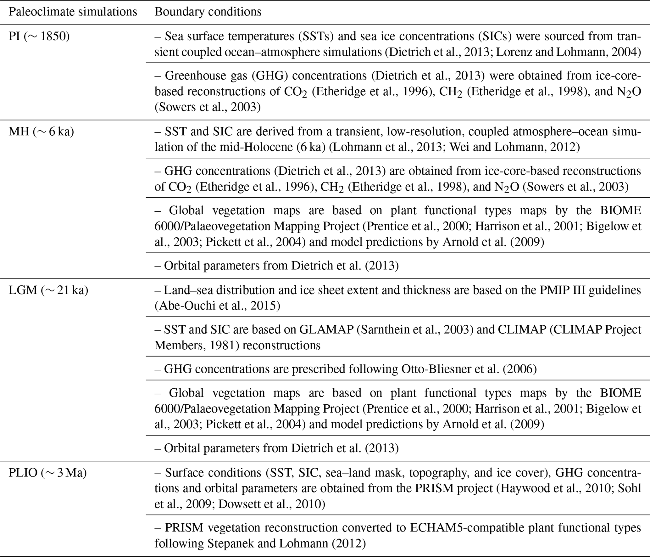
^* (SST: sea surface temperature; SIC: sea ice concentration; GHG: greenhouse gas; PMIP III: Paleoclimate Modelling Intercomparison Project, phase 3; PRISM: Pliocene Research, Interpretation and Synoptic Mapping).

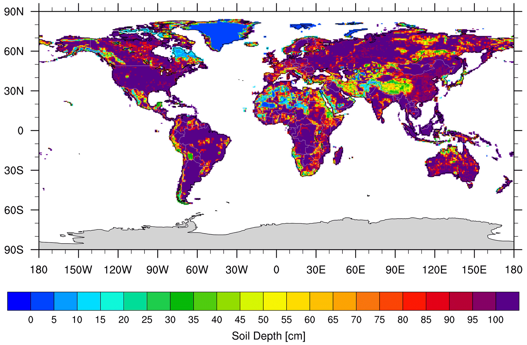
Figure 1 Soil depth map from the Harmonized World Soil Database (HWSD, version 1.2) used in this study (Wieder et al., 2014). Due to the paucity of some data inputs for paleoclimate time slices (e.g., soil thickness, rock properties, hydrology), the simulations assume present-day values.

3 Methods

In this section we present the pre-processing of GCM paleotemperature data for the calculation of mean annual temperatures (MATs) and the half-amplitude of annual temperature variations (T_a). This is followed by the description of the models (simpler to complex) that were applied to generate first-order (global) estimation of annual depth-integrated FCI for selected Cenozoic time slices.

3.1 Pre-processing of GCM simulation temperature data

We calculated the mean annual land surface temperatures (MAT) to serve as input for subsequent calculations and a reference for differences in global paleoclimate. The MATs for the paleoclimate GCM experiments (PLIO, LGM, MH, and PI) were calculated (Fig. 2) from each of the simulations' 15 years of daily land surface temperature values. In addition, the half-amplitude of annual surface temperature variations (T_a) was extracted at all surface grid locations for all years (Fig. 3). We use the MAT for ground surface temperature in subsequent calculations, following Anderson et al. (2013), Marshall et al. (2015), and Rempel et al. (2016). The maxima and minima for global average MATs and T_a values for all the time slices are shown in Table 2.

Table 2 MAT and T_a (for ground surface temperature) for pre-industrial, mid-Holocene, Last Glacial Maximum, and Pliocene simulations.

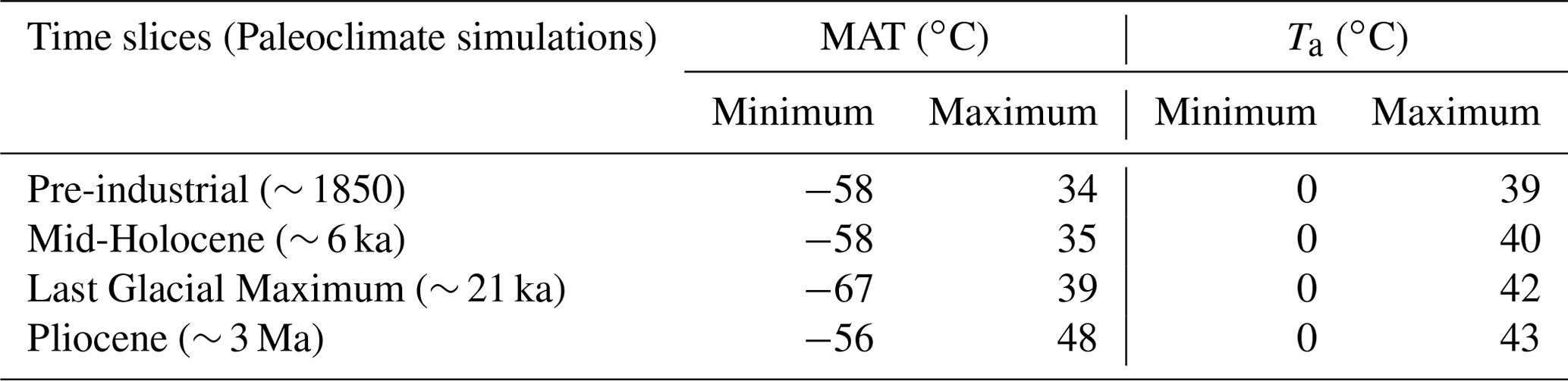
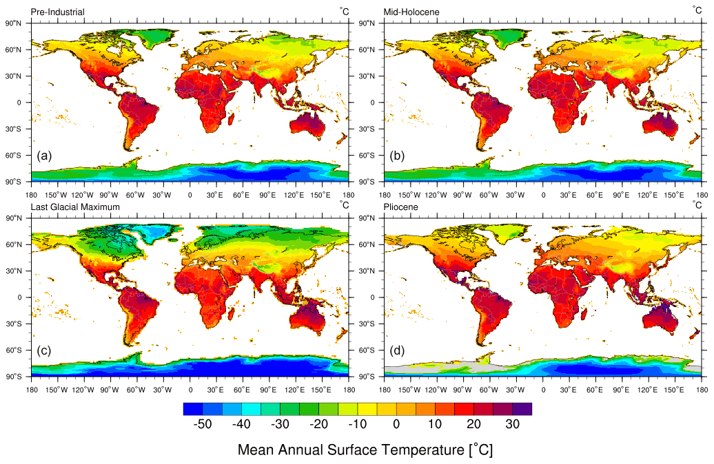
Figure 2 Mean annual surface temperature maps (15-year average) from the ECHAM5 GCM simulations for the pre-industrial (a), mid-Holocene (b), Last Glacial Maximum (c), and mid-Pliocene (d) (unit: ^∘C). These are calculated from GCM simulation output of Mutz et al. (2018) and Mutz and Ehlers (2019).

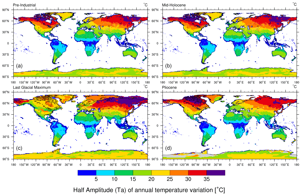
Figure 3 Half-amplitude of annual temperature variation (15-year average) for the pre-industrial (a), mid-Holocene (b), Last Glacial Maximum (c), and Pliocene (d) (unit: ^∘C). These are calculated from GCM simulation output of Mutz et al., (2018) and Mutz and Ehlers (2019).

The calculation of temporally varying subsurface temperatures follows the approach of Hales and Roering (2007) and uses the analytical solution for the one-dimensional heat conduction equation (Turcotte and Schubert, 2014) forced with daily temperatures following sinusoidal variations. While daily paleotemperatures can be obtained from Mutz et al. (2018), the daily variations produced by the GCM cannot be validated as well as seasonal or annual means. To avoid overinterpretation of the GCM simulations, we refrained from using daily paleotemperatures from Mutz et al. (2018) and instead use sinusoidal daily temperatures. Temperature variations with depth and time were calculated at each GCM grid point as

$$\begin{array}{}\text{(1)}& T\left(z,t\right)=\mathrm{MAT}+T_{\mathrm{a}}\cdot e^{-z\sqrt{\frac{\mathit{\pi }}{\mathit{\alpha }{P}_y}}}\cdot \sin \left({\displaystyle \frac{\mathrm{2}\mathit{\pi }t}{P_y}}-z\sqrt{{\displaystyle \frac{\mathit{\pi }}{\mathit{\alpha }{P}_y}}}\right),\end{array}$$

where T represents daily subsurface temperature at depth z (m) and time t (days in a year), MAT and T_a represent mean annual surface temperature and half-amplitude of annual temperature variation, respectively, P_y is the period of the sinusoidal cycle (1 year), and α is the thermal diffusivity. Thermal diffusivity values near the Earth's surface can range from 1–$\mathrm{2}\times {\mathrm{10}}^{-\mathrm{6}}$ m² s⁻¹ for most rocks (Anderson, 1998) and range 7–$\mathrm{10}\times {\mathrm{10}}^{-\mathrm{7}}$ m² s⁻¹ for other Earth materials comprising the overlying sediment layer (Eppelbaum et al., 2014). In this study, we used a thermal diffusivity of $\mathrm{1.5}\times {\mathrm{10}}^{-\mathrm{6}}$ m² s⁻¹ for bedrock and $\mathrm{8}\times {\mathrm{10}}^{-\mathrm{7}}$ m² s⁻¹ for the overlying sediment layer. The maximum depth investigated here is 20 m, as it is slightly deeper than the maximum frost penetration depth of ∼ 14 m reported by Hales and Roering (2007).

The calculation of subsurface temperatures was discretized into 200 depth intervals from the surface to the maximum depth of 20 m. Smaller depth intervals (∼ 1 cm) were used near the surface and large intervals (∼ 20 cm) at greater depths because the FCI is expected to change most dramatically near the surface and dampen with depth due to thermal diffusion (Andersen et al., 2015).

3.2 Estimation of frost cracking intensity

We applied three different approaches (models) with different levels of complexity to estimate global variations in frost cracking during different past climates (Fig. 4; Andersen et al., 2015; Anderson, 1998; Hales and Roering, 2007). The models use predicted ground surface temperatures from each grid cell in the GCM to calculate subsurface temperatures and FCI. We then calculate differences between the FCI from the PI reference simulation and the FCI predicted for the PLIO, LGM, and MH time slices to assess relative change in FCI over the late Cenozoic. The conceptual diagram (Fig. 4) illustrates differences in the models used in our study, which are discussed in detail in Sect. 3.2.1–3.2.3. Models 1–3 successively increase in complexity and consider more factors. The approach of Andersen et al. (2015), referred to here as Model 3, is the most recent and complex in its consideration of the processes (e.g., effect of soil cover on FCI) that are relevant for frost cracking. Given this, we focus our presentation of results in the main text here on Model 3, but for completeness we describe differences of Model 3 from earlier models (1–2) below . For brevity, results from the earlier models are presented in the Supplement. A flowchart illustrating our methods is presented in Fig. 5. Similar to previous studies, the hydrogeological properties of the bedrock (i.e., infiltration, water saturation, porosity, and permeability) are ignored in this study. This approach provides a simplified means for estimating the FCI for underlying bedrock at a global scale.

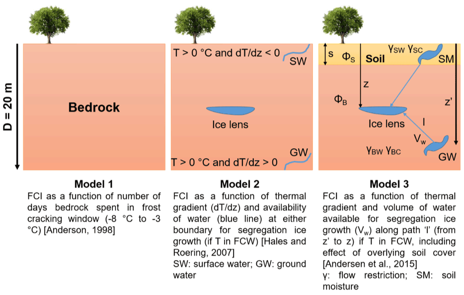
Figure 4 Conceptual diagram of the models (1, 2, and 3) used for estimating FCI (T: temperature; dT $/$ dz: thermal gradient; SW: surface water; GW: groundwater; SM: soil moisture; s: sediment thickness; φS: soil porosity, 0.02; φB: bedrock porosity, 0.3).

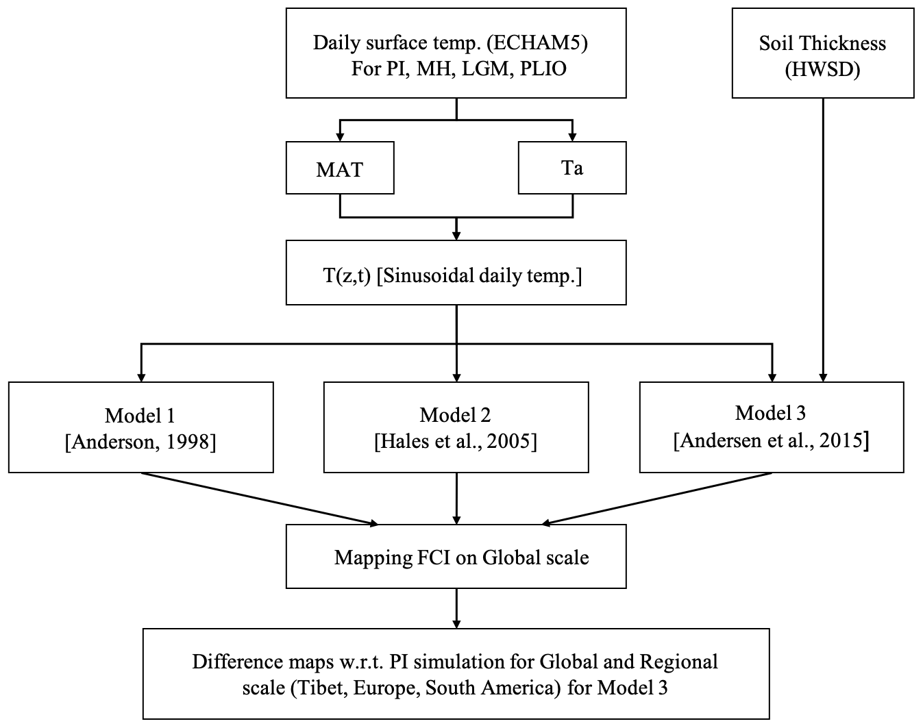
Figure 5 Flowchart describing the methods used in the study based on daily surface temperature simulated by the ECHAM GCM and soil thickness data from HWSD v1.2. Abbreviations: MAT – mean annual temperature; T_a – half-amplitude of annual temperature variation; T (z,t) – subsurface temperature at depth z and time t; FCI – frost cracking intensity.

3.2.1 Model 1: frost cracking intensity as a function of time spent in the frost cracking window (FCW)

Model 1 represents the simplest approach and applies the method of Anderson (1998). In our application of this model, we use a more representative thermal diffusivity value for rocks of $\mathrm{1.5}\times {\mathrm{10}}^{-\mathrm{7}}$ m² s⁻¹. The previous study applied a diffusivity specific to granitic bedrock. Furthermore, the boundary conditions of a low rock surface albedo (≤ 0.1) and presence of a high atmospheric transmissivity (≥ 0.9) on the surface were relaxed, as surface temperatures were used in our study instead of near-surface air temperatures.

For our implementation of Model 1, we applied Eq. (1) for sinusoidal varying daily temperatures at the surface and calculated temperatures up to 20 m depth. The number of days spent in the FCW (−8 to −3 ^∘C) for each depth interval was calculated over a period of 1 year for all time slices (PI, MH, LGM, and PLIO):

$$\begin{array}{}\text{(2)}& \mathrm{FCI}\left(z\right)=\left\{\begin{array}{l}N\left(z\right),\mathrm{if}-\mathrm{8}{}^{\circ }\mathrm{C}<T\left(z,t\right)<-\mathrm{3}{}^{\circ }\mathrm{C}\\ \mathrm{0},\mathrm{else},\end{array}\right.\end{array}$$

where FCI (z) is the frost cracking intensity at depth z. N(z) indicates the number of days the bedrock (at depth z) spends in the FCW over a period of 1 year.

Estimation of frost cracking intensity for each location included depth averaging of the FCI such that

$$\begin{array}{}\text{(3)}& \mathrm{F}\text{Ć}\mathrm{I}={\displaystyle \frac{\mathrm{1}}{D}}{\int }_{\mathrm{0}}^D\mathrm{FCI}\left(z\right)\mathrm{d}z,\end{array}$$

where FĆI is the integrated frost cracking intensity to a depth of D= 20 m. The unit of integrated frost cracking intensity in this model is days. The FCI values are calculated for all model years separately and then averaged over the total time (15 years) for each paleoclimate time slice.

3.2.2 Model 2: frost cracking intensity as a function of subsurface thermal gradients

Model 2 applies the approach of Hales and Roering (2007) to estimate FCI using climate-change-driven variations in subsurface thermal gradients. This approach extends the work of Anderson (1998) with the additional consideration of segregation ice growth. Segregated ice growth is attributed to the migration of liquid water to colder regions in shallow bedrock, accumulating in localized zones to form ice lenses and inducing weathering (Walder and Hallet, 1985).

To facilitate ice segregation growth, the model assumes the availability of liquid water (T > 0 ^∘C) at either boundary (z= 0 or z= 20 m), with a negative thermal gradient for a positive surface temperature and a positive thermal gradient for the positive lower boundary (z= 20 m) temperature. This implementation supports frost cracking in the bedrock with temperatures between −8 and −3 ^∘C (Hallet et al., 1991). In the case of permafrost areas, MAT is always negative, but as sinusoidal T(z,t) is calculated based on MAT and T_a, a positive T (> 0 ^∘C) may occur during warmer days of the year. In addition, T_a is higher for higher latitudes (Fig. 3), which are more prone to frost cracking. The model is described as follows:

$$\begin{array}{}\text{(4)}& {\displaystyle }\mathrm{FCI}\left(z,t\right)=\left\{\begin{array}{l}\left|\frac{\mathrm{d}T}{\mathrm{d}z}\right|\left(z,t\right),\mathrm{if}-\mathrm{8}{}^{\circ }\mathrm{C}<T\left(z,t\right)<-\mathrm{3}{}^{\circ }\mathrm{C}\\ \mathrm{0},\mathrm{else},\end{array}\right.\text{(5)}& {\displaystyle }\mathrm{F}\text{Ć}\mathrm{I}={\int }_{\mathrm{0}}^D{\int }_{\mathrm{0}}^{P_y}\mathrm{FCI}\left(z,t\right)\mathrm{d}t\mathrm{d}z,\end{array}$$

where FCI (z,t) is the frost cracking intensity at depth z and time t. It is an index for the absolute value of the thermal gradient at that particular depth and time that fulfills the conditions defined above.

In Eq. (5), FĆI represents the integrated FCI for a geographic location. More specifically, the FCI is integrated over 1 year at each depth and then integrated for all depth elements. D represents depth (20 m), Py is a period of the sinusoid (1 year), dt is the time interval (1 d), and dz is the depth interval, as described in Sect. 3.1. The unit of integrated frost cracking intensity, in this case, is degrees Celsius (^∘C).

3.2.3 Model 3: frost cracking intensity as a function of thermal gradients and sediment thickness

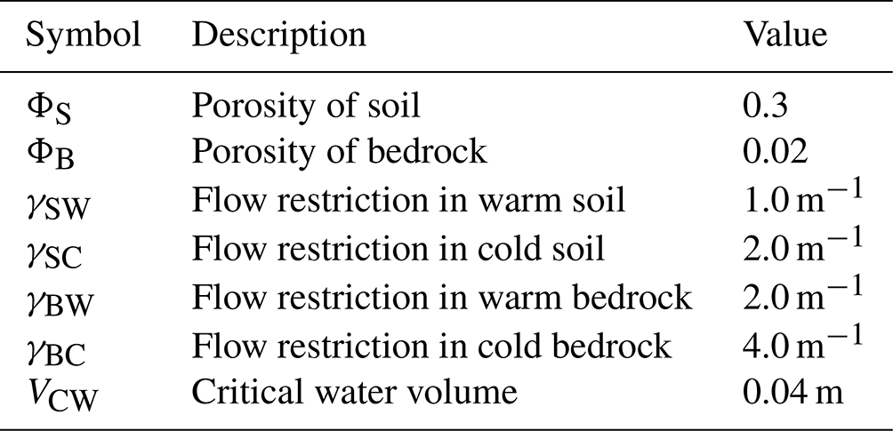
In the final (most complex) approach used in this study, the effect of an overlying soil layer (Fig. 1) is considered in addition to the subsurface thermal gradient variations with depth. This model applies the approach of Andersen et al. (2015), which extends the work of Hales and Roering (2007) and Anderson et al. (2013). The model assumptions are similar to the previous approaches. For segregation ice growth, it additionally considers the influence of the volume of water available in the proximity of an ice lens. The parameters used in Model 3 are listed below (Table 3).

Table 3 Input parameters for Model 3 (Andersen et al., 2015).

In Model 3, frost cracking intensity is estimated as a product of the thermal gradient and volume of water available (V_W) for segregation ice growth at each depth element such that

$$\begin{array}{}\text{(6)}& \mathrm{FCI}\left(z,t\right)=\left\{\begin{array}{l}\left|\frac{\mathrm{d}T}{\mathrm{d}z}\left(z,t\right)\right|V_{\mathrm{W}}\left(z\right),\mathrm{if}-\mathrm{8}{}^{\circ }\mathrm{C}<T\left(z,t\right)<-\mathrm{3}{}^{\circ }\mathrm{C}\\ \mathrm{0},\mathrm{else}\end{array}\right.,\end{array}$$

where FCI (z,t) is the frost cracking intensity in bedrock at depth z and time t, and V_W(z) is the volume of water available for segregation ice growth. V_W(z) is estimated at each depth (z) by integrating the occurrence of unfrozen water along a path l, starting at depth z and following a positive thermal gradient towards the ice lens. The volume of available water (V_W(z)) and total flow restriction (Γ(z^′)) between the depth of occurrence of water (z^′) and the location of segregation ice growth (z) are calculated using Eqs. (7) and (8), respectively (Andersen et al., 2015):

$$\begin{array}{}\text{(7)}& {\displaystyle }{V}_{\mathrm{W}}\left(z\right)={\int }_l\mathit{\varphi }\left(z^{\prime }\right)w_f\left(z^{\prime }\right)e^{-\mathrm{\Gamma }\left(z^{\prime }\right)}\mathrm{d}{z}^{\prime },\text{(8)}& {\displaystyle }\mathrm{\Gamma }\left(z^{\prime }\right)={\int }_z{{}^{\prime }}^z\mathit{\gamma }\left(z^{\prime \prime }\right)\mathrm{d}{z}^{\prime \prime },\end{array}$$

where l is the distance from depth z to the surface, lower boundary, or an interface where the thermal gradient changes sign (from positive to negative or vice versa). The penalty function $e^{-\mathrm{\Gamma }\left(z^{\prime }\right)}$ (Anderson et al., 2013) is a function of the total flow restriction (Γ(z^′)) at depth z^′. Since segregation ice growth is exhibited at sub-zero temperatures (below −3 ^∘C) and liquid water is available at positive temperatures (T > 0 ^∘C), water must migrate through a mixture of frozen and unfrozen soil or the bedrock. The variables γ_SW, γ_SC, γ_BW, and γ_BC (defined in Table 3) represent the flow restriction parameters and were used in the model to approximate a range of permeabilities (Andersen et al., 2015) but do not explicitly simulate water transport. However, it is unclear if the inclusion of the penalty function leads to a better representation of frost cracking processes. Therefore, we conducted two sets experiments for Model 3 that were conducted with and without the penalty function and are presented in Sect. 4.1 and 4.2, respectively.

The soil porosity (φ_S= 0.3) is assumed to be higher than that of bedrock (φ_B= 0.02). V_W(z) is expected to be high due to the presence of unfrozen soil in the proximity of frozen bedrock. Since Model 3 limits the positive effects of V_W to a critical water volume V_CW (Table 2, i.e., if V_W > V_CW, then V_W= V_CW), the expected high (> V_CW) values for V_W will not affect frost cracking any further.

Lastly, the integrated frost cracking intensity FĆI across Earth's terrestrial surface was calculated by depth integration of the FCI averaged over a period of 1 year (Anderson et al., 2013):

$$\begin{array}{}\text{(9)}& \mathrm{F}\text{Ć}\mathrm{I}={\displaystyle \frac{\mathrm{1}}{P_y}}\underset{\mathrm{0}}{\overset{P_y}{\int }}\underset{\mathrm{0}}{\overset{D}{\int }}\mathrm{FCI}\left(z,t\right)\mathrm{d}z\mathrm{d}t,\end{array}$$

where P_y is 1 year and D is the maximum depth investigated (20 m). The unit of integrated FCI in this model is ^∘C m. Integrated FCI is calculated for each of the GCM simulation's model years and then averaged over the total number of years (15 years).

4 Results

In the following, we document the general trends in the estimated FCI from Model 3 (Andersen et al., 2015) for all the paleoclimate time slices (PI, MH, LGM, PLIO) based on the coupling of the above models to GCM output for these time slices. We present the results for the experiments conducted with and without the penalty function separately in Sect. 4.1 and 4.2, respectively. The FCI distribution is masked for the glaciated regions during specific paleoclimate time slices, as the surface covered under ice sheets is disconnected from atmospheric processes (Grämiger et al., 2018). In the PLIO results, the regions that experienced Pleistocene glaciation are masked with the LGM glacier cover, as the assumption of comparable soil depths in these regions is heavily violated. Since spatial and temporal variations in frost cracking do not vary much between the three approaches, for brevity we focus our presentation of results on the most recent (Model 3 – Andersen et al., 2015) approach. The results of simpler approaches (Models 1, 2; Anderson, 1998, and Hales and Roering, 2007) are presented in the Supplement.

4.1 Model 3 – Scenario 1: FCI as a function of thermal gradient and soil thickness (with penalty function)

In this scenario, we estimate the global FCI distribution using Model 3 (Andersen et al., 2015) with the penalty function, which makes FCI dependent on the distance to water. The predicted global sum of FCI is greatest for the LGM (∼ 1025 ^∘C m), followed by the MH (∼ 940 ^∘C m) and PI (∼ 835 ^∘C m) simulations. The correlation between FCI values and T_a is high (Pearson r: between 0.8 and 0.89) and statistically significant (using the 95 % level as a threshold to determine significance). On the other hand, the correlation between FCI and MATs is good in the LGM (Pearson r: −0.68), moderate in the PI and MH (Pearson r: −0.3 to −0.4), and poor in the PLIO (Pearson r: −0.04).

For all paleoclimate time-slice experiments, the FCI predicted by Model 3 is in the range of 0–0.22 ^∘C m at higher latitudes (30–80^∘ N and 45–60^∘ S) (Fig. 6). The maximum FCI values are observed in the higher latitudes (50–80^∘ N) and show the same pattern as variations in T_a when T_a exceeds 30 ^∘C. In the PI and MH simulations, the highest FCI is observed in North America (40–55^∘ N and 70–80^∘ N) and Eurasia (35–50^∘ N, 55–80^∘ E and 55–80^∘ N, 80–180^∘ E), with values ranging from ∼ 0.08 ^∘C m to ∼ 0.2 ^∘C m. Low FCI can be observed in South America, with values between 0.02 ^∘C m and 0.05 ^∘C m. This is consistent with results from Models 1 and 2 (see Supplement). In the LGM simulation, the highest FCI values are observed in Alaska, Turkmenistan, Uzbekistan, eastern China, and northeastern latitudes in Eurasia (70–80^∘ N, 105–180^∘ E) with values ranging from ∼ 0.08 to ∼ 0.2 ^∘C m. In the Andes of South America, the frost cracking activity is restricted to the geographical range of 12–55^∘ S. The highest South American FCI values (∼ 0.15 to ∼ 0.22 ^∘C m) are predicted for the southern part of the continent (40–50^∘ S).

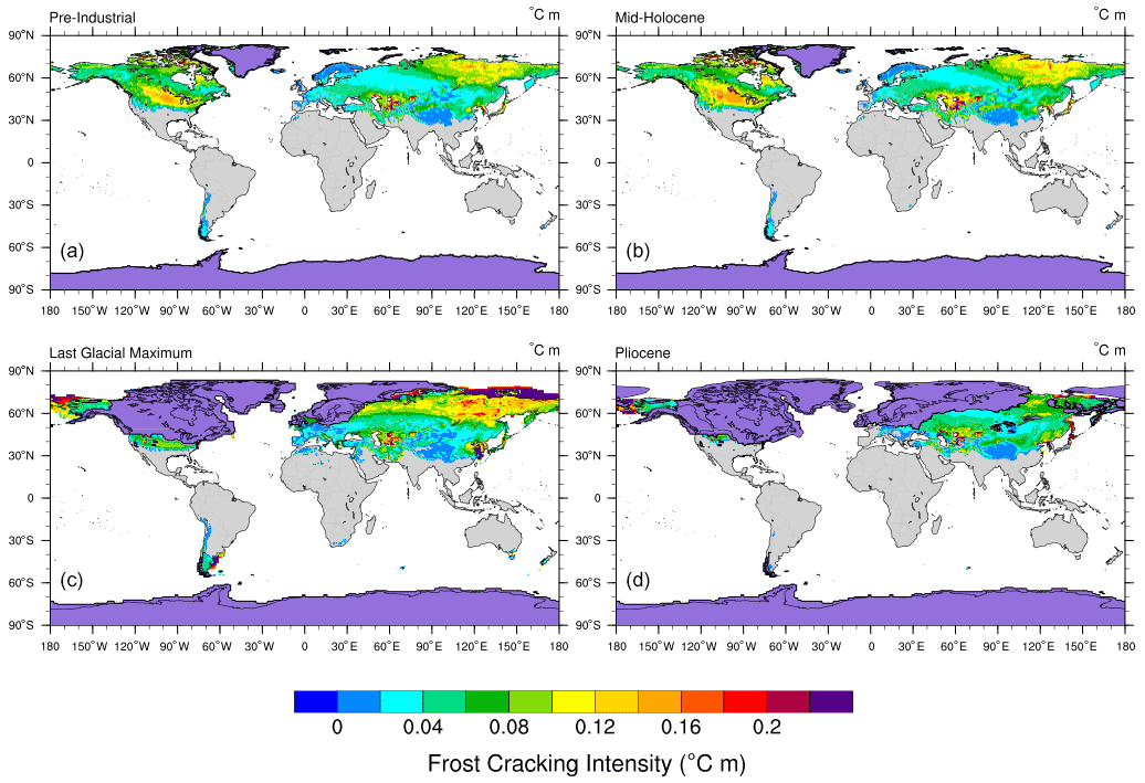
Figure 6 Model 3 (Scenario 1) predicted integrated FCI as a function of thermal gradient and sediment thickness (with the penalty function) for pre-industrial (a), mid-Holocene (b), Last Glacial Maximum (c), and mid-Pliocene (d) times (unit: ^∘C m). The grey areas in plots indicate the absence of frost cracking. For all time slices, the regions covered by ice were removed from the calculation and are highlighted in violet (Bracannot et al., 2012). For the PLIO results, the maximum Quaternary ice extent (Batchelor et al., 2019) is used, since the assumption of modern soil depth is heavily violated in these regions.

In the mid-Pliocene, the maximum FCI values are predicted in the higher latitudes, i.e., Alaska (∼ 0.15 ^∘C m to ∼ 0.22 ^∘C m). Moderately high values are predicted for the northern latitudes of Eurasia (0.05–0.16 ^∘C m). Overall, the magnitude of mid-Pliocene FCI is lower than that of all other investigated time slices. The only exceptions are some high-latitude regions (e.g., Alaska) that exhibit locally higher FCI values in the mid-Pliocene relative to the PI. Negligible frost cracking is predicted for South America, which is consistent with the results of Model 1 (Anderson, 1998).

For all the time slices, regions with positive MATs (0 to 15 ^∘C) exhibit higher values of FCI where the sediment cover is thinner (e.g., middle East Asia). In contrast, predictions of FCI in regions with negative MATs (−5 to −20 ^∘C) and high T_a (30 to 40 ^∘C) tend to be higher where sediment cover is thicker (e.g., northeastern Eurasia).

4.2 Model 3 – Scenario 2: FCI as a function of thermal gradient and soil thickness (without penalty function)

In this scenario, we estimate global FCI distribution using Model 3 (Andersen et al., 2015) without applying the penalty function (Fig. 7). The highest magnitude of frost cracking intensity is simulated for the PLIO (∼ 53 ^∘C m), followed by the MH (∼ 47 ^∘C m), PI (∼ 45 ^∘C m), and LGM (∼ 43 ^∘C m). However, the maximum global sum of FCI is observed in the MH (∼ 314 000 ^∘C m), followed by the PI (∼ 303 000 ^∘C m) and LGM (∼ 238 000 ^∘C m) simulations. Similar to the observations in Model 2 (see Supplement Fig. S2), the FCI distribution is negatively correlated with MATs (Pearson r: between −0.4 and −0.5) and T_a (Pearson r: between 0.9 and 0.95). These correlations are significant (using the 95 % threshold to determine significance).

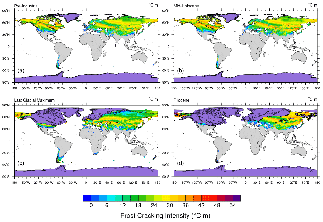
Figure 7 Model 3 (Scenario 2) predicted integrated FCI as a function of thermal gradient and sediment thickness (without the penalty function) for pre-industrial (a), mid-Holocene (b), Last Glacial Maximum (c), and mid-Pliocene (d) times (unit: ^∘C m). The grey areas in plots indicate the absence of frost cracking. For all time slices, the regions covered by ice were removed from the calculation and are highlighted in violet (Bracannot et al., 2012). For the PLIO results, the maximum Quaternary ice extent (Batchelor et al., 2019) is used, since the assumption of modern soil depth is heavily violated in these regions.

In the PI simulations, the maximum FCI values are predicted for the middle to high latitudes (i.e., FCI: 21–44 ^∘C m in 40–70^∘ N) of North America and Eurasia. Low to moderate frost cracking is predicted for South America (i.e., FCI: 6–18 ^∘C m in 20–55^∘ S). The MH simulations predict a similar FCI pattern and FCI values that are slightly higher than in the PI (e.g., FCI: 21–47 ^∘C m in 40–70^∘ N).

In the LGM simulation, major portions of North America and Europe are covered by ice sheets and thus excluded from our frost cracking models. The simulations yield maximum FCI values for Alaska (i.e., 21–44 ^∘C m) and the middle to high latitudes in Asia (i.e., FCI: 14–42 ^∘C m in 35–65^∘ N), moderate FCI values in the periglacial regions in North America (i.e., FCI: 18–33 ^∘C m in 35–42^∘ N), and low FCI values in South America (i.e., FCI: 4–18 ^∘C m in 15–55^∘ S). In the PLIO simulation, major frost cracking activity is predicted for Alaska (i.e., 21–48 ^∘C m) and the northern latitudes of Asia (i.e., FCI: 18–48 ^∘C m in 30–80^∘ N). We do not observe any significant frost cracking in Europe, North America, and South America in the PLIO simulations.

5 Discussion

In this section, we synthesize and interpret the global results of all the models, including scenarios with and without the penalty function in Model 3. For brevity, we limit our discussion of regional variations to Tibet, Europe, and South America. For other regional areas of interest to readers, the data used in the following figures are available for download (see the “Code and data availability” section). Our presentation of selected regional areas is followed by the comparison of modeled FCI with published field observations. We also compare the model outcomes of all the three models used in the study. Finally, we discuss the study's limitations.

5.1 Synthesis and interpretation

This section comprises the synthesis and interpretation of the global trends in FCI values predicted by Models 1–3 for the investigated paleoclimate simulations (PI, MH, LGM, and PLIO). In all the paleoclimate simulations, high values of FCI in northern latitudes (60–80^∘ N) in Eurasia and North America coincide with lower MATs in the range of −25 to −5 ^∘C and very high T_a values in the range of 30 to 40 ^∘C. FCI in areas with negative MATs is mainly controlled by the T_a values, as higher T_a and high thermal gradients are predicted in the subsurface and facilitate ice segregation growth (Hales and Roering, 2007; Hallet et al., 1991; Murton et al., 2006; Walder and Hallet, 1985).

We also calculated the global sum of FCI for all paleoclimate time slices to determine which Cenozoic timescale is most important for frost cracking in each model. Furthermore, we compare the global sum of FCI in MH and LGM to that of PI simulations. We do not compare the global sum of FCI in PLIO simulations, as it might be heavily affected by masking the glaciated regions. Model 1 predicts a maximum FCI for the PI. These are 3.8 % and 27 % higher than the FCI values in the MH and LGM simulations, respectively. In Model 2, MH experiences maximum FCI, which is 2.4 % higher than in the PI, while FCIs in the LGM simulation are 15 % lower than in the PI. In Model 3 (Scenario 1), the LGM and MH experience FCI values that are 22 % and 12 % higher than in the PI simulation. In Model 3 (Scenario 2), MH experiences the maximum FCI, which is 3.5 % higher than in the PI, while FCI in the LGM simulation is 21 % lower than in the PI. The global sum of FCI estimates is consistent between Models 1, 2, and 3 (Scenario 2) and suggests that maximum frost cracking (weathering) occurred during inter-glacial periods (i.e., MH and PI), while the glacial period (LGM) experienced comparatively less frost cracking. The above predictions for frost cracking (e.g., in Models 1, 2, and 3 – Scenario 2) are inconsistent with studies of global weathering fluxes during glacial and inter-glacial periods, which reported an increase in weathering of ∼ 20 % in the LGM (compared to the present) (Gibbs and Kump, 1994; Ludwig et al., 1999). This pattern is, however, predicted by Model 3 (Scenario 1) for which the maximum in global frost cracking is predicted for the glacial period (LGM). More specifically, Model 3 (Scenario 1) predicts an increase of 22 % in the global sum of FCI during LGM from PI values. This observation is also consistent with the findings of a similar work by Marshall et al. (2015), which suggested that frost weathering was higher during the LGM than today in unglaciated regions. These results highlight the importance of the penalty function (i.e., dependency of FCI on distance to water) in first-order (global) estimations of FCI.

5.2 Influence of past climate on FCI on a global scale

We have investigated the influence of climate change on frost cracking on different spatial scales and through geologic time using three different frost cracking models (Anderson, 1998; Hales and Roering, 2007; Andersen et al., 2015) and paleoclimate GCM simulations (Mutz et al., 2018). Our results for Model 3 are presented as maps showing time-slice-specific FCI anomalies relative to the PI climate simulation on a global scale (Figs. 8a, 9a, 10a) and in Europe (Figs. 8b, 9b, 10b), Tibet (Figs. 8c, 9c, 10c), and South America (Figs. 8d, 9d, 10d). Furthermore, we highlighted where continental ice was located for all time slices (PI, MH, LGM) or where Pleistocene ice cover could result in a violation of our assumption of modern soil thickness (PLIO) (Figs. 8–10). This was done to prevent unmerited regional comparisons of simulated FCI.

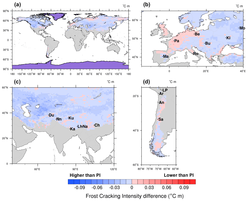
Figure 8 Differences between (Model 3) predictions of pre-industrial and mid-Holocene long-term FCI means (unit: ^∘C m) for (a) the entire Earth surface, (b) Europe, (c) South Asia, and (d) South America. Glacial cover is highlighted in violet. City abbreviations are as follows. Tibet: Du – Dushambe, Nn – Srinagar, Ku – Xinjiang, Ka – Kathmandu, Lh – Lhasa, Na – Namcha Barwa, Ch – Chenshangou; Europe: Pa – Paris, Be – Berlin, Mo – Moscow, Ki – Kyiv, Ro – Rome, Bu – Budapest, Ma – Madrid; South America: LP – La Paz, Ar – Arica, An – Antofagasta, Sa – Santiago. The regions covered by ice were removed from the calculation and are highlighted in violet (Bracannot et al., 2012).

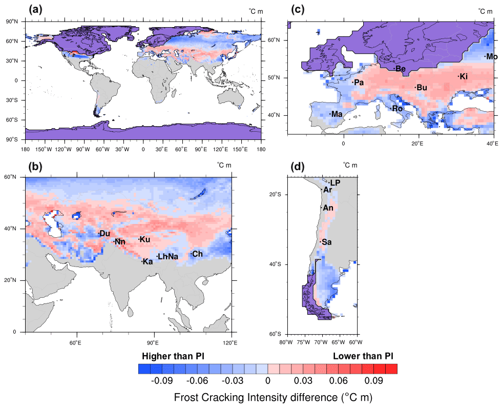
Figure 9 Differences between (Model 3) predictions of pre-industrial and Last Glacial Maximum long-term FCI means (unit: ^∘C m) for (a) the entire Earth surface, (b) Europe, (c) South Asia, and (d) South America. Glacial cover is highlighted in violet. City abbreviations are as follows. Tibet: Du – Dushambe, Nn – Srinagar, Ku – Xinjiang, Ka – Kathmandu, Lh – Lhasa, Na – Namcha Barwa, Ch – Chenshangou; Europe: Pa – Paris, Be – Berlin, Mo – Moscow, Ki – Kyiv, Ro – Rome, Bu – Budapest, Ma – Madrid; South America: LP – La Paz, Ar – Arica, An – Antofagasta, Sa – Santiago. The regions covered by ice were removed from the calculation and are highlighted in violet (Bracannot et al., 2012).

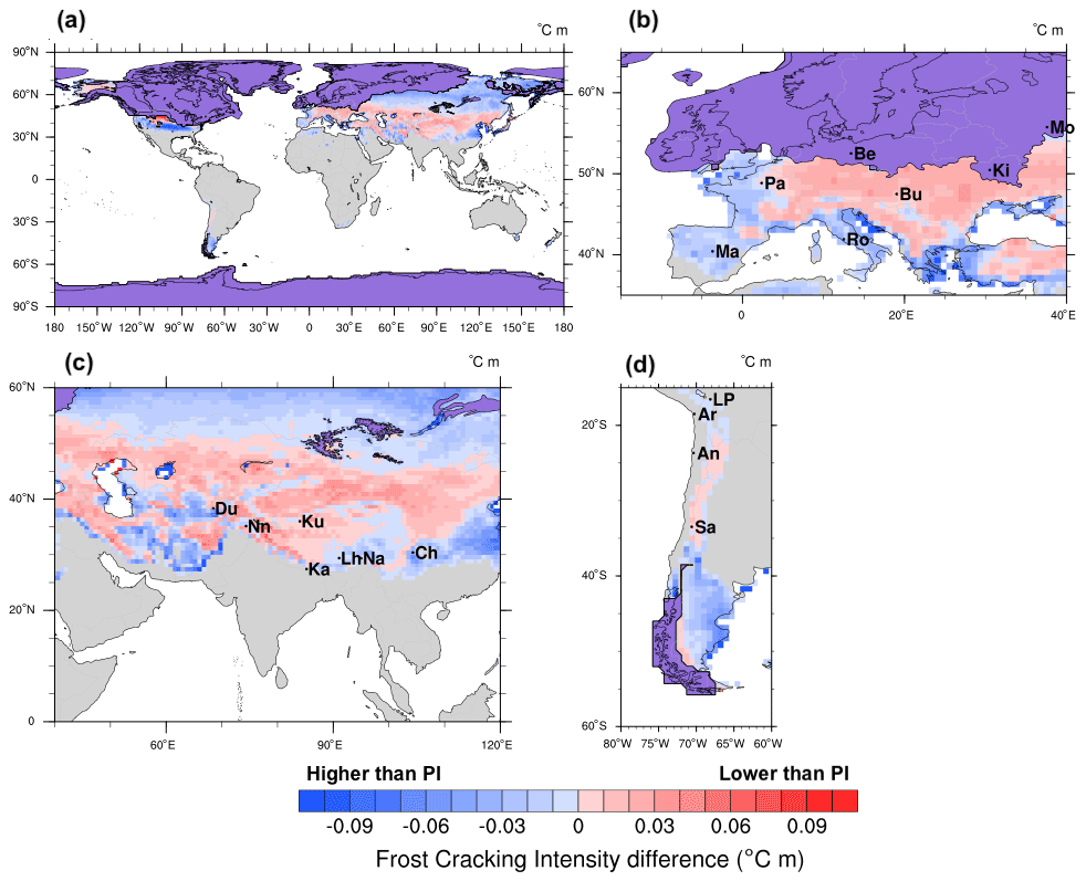
Figure 10 Differences between (Model 3) predictions of pre-industrial and Pliocene long-term FCI means (unit: ^∘C m) for (a) the entire Earth surface, (b) Europe, (c) South Asia, and (d) South America. Maximum Pleistocene glacial cover is highlighted in violet. City abbreviations are as follows. Tibet: Du – Dushambe, Nn – Srinagar, Ku – Xinjiang, Ka – Kathmandu, Lh – Lhasa, Na – Namcha Barwa, Ch – Chenshangou; Europe: Pa – Paris, Be – Berlin, Mo – Moscow, Ki – Kyiv, Ro – Rome, Bu – Budapest, Ma – Madrid; South America: LP – La Paz, Ar – Arica, An – Antofagasta, Sa – Santiago. The regions covered by ice were removed from the calculation and are highlighted in violet (Bracannot et al., 2012).

The differences in FCI between the PI and MH climate simulations are in the range of −0.04 to 0.02 ^∘C m on a global scale (Fig. 8a). The MH simulation yields higher FCI values for most regions except for parts of northern Asia, mid-western Europe, mid-North America, the Andes Mountains, and parts of Alaska and Tibet. These differences may be attributed to the slight changes in MATs in these regions. The PI–MH comparisons for Europe (Fig. 8b) reveal very small deviations in MH-FCI from PI conditions (ΔFCI $\approx -\mathrm{0.02}$ to 0.02 ^∘C m). These changes are negative in western Europe (including areas near the cities of Paris, Berlin, and Rome) and positive in eastern Europe (including Budapest, Kyiv, and Moscow). Tibet exhibits only small (∼ 0.02 ^∘C m), predominantly positive MH-FCI deviations from PI conditions (Fig. 8c). The magnitude of PI–MH FCI differences in southwestern South America (Fig. 8d) is similar to that in other regions (ΔFCI ≈ −0.02 to 0.02 ^∘C m).

5.2.1 Differences in FCI between PI and LGM climate simulations

The differences in FCI between PI and LGM on a global scale (Fig. 9a) are highest in the middle to high latitudes (∼ 42^∘ N) in North America (ΔFCI ≈ 0.08 ^∘C m) and northern Asia (∼ 75^∘ N) (ΔFCI ≈ 0.07 ^∘C m). The close proximity of these regions to the glacier cover in the LGM highlights the possibility of the presence of periglacial environments that support frost cracking (Marshall et al., 2015) during the PI. This is also observed in the middle to high latitudes in Asia (30–50^∘ N) (ΔFCI ≈ 0.04 ^∘C m), which may be attributed to the positive MATs in this region during the PI simulation.

However, in the higher latitudes of Asia (∼ 50 to 70^∘ N) and South America (∼ 40 to 50^∘ S), the LGM experiences more frost cracking than the PI (ΔFCI ≈ −0.03 to −0.06 ^∘C m). This can be attributed to higher T_a values (Fig. 3) in these regions during the LGM. In central Europe (Fig. 9b), including Paris, Budapest, and Kyiv, the PI shows higher FCI (ΔFCI ≈ 0.02–0.06 ^∘C m) than the LGM. On the other hand, the LGM simulations predict higher FCI (ΔFCI ≈ −0.02 to −0.06 ^∘C m) in southern Europe (including Madrid and Rome). Overall, the Tibetan Plateau experiences higher FCI values (ΔFCI ≈ 0.06 ^∘C m) during the PI (Fig. 9c). Only in the eastern part of Tibet, near Lhasa, are LGM-FCI values higher (ΔFCI ≈ 0.04 ^∘C m). In South America (Fig. 9d), the LGM yields lower FCI values (ΔFCI ≤ 0.06 ^∘C m) in the Andes Mountains, and the PI simulation yields lower FCI values (ΔFCI ≥ −0.06 ^∘C m) in the east of the Andes Mountains in the southern part of the region (40–50^∘ S).

5.2.2 Differences in FCI between PI and PLIO climate simulations

Frost cracking is higher in the PI than in the PLIO (Fig. 10a) (ΔFCI ≈ 0.04–0.08 ^∘C m) in the middle to high latitudes of Europe and North America (35–55^∘ N), as well as in higher latitudes in Asia (50–80^∘ N). This can be attributed to the warmer climate during PLIO and high T_a (Fig. 3) in the PI simulation. However, the PLIO exhibits marginally higher frost cracking in some regions of Asia and Alaska, where MATs are in the range of 0–5 ^∘C.

In central to southern Europe, including Madrid, Paris, Rome, Budapest, and Kyiv, PI-FCI values are moderate (ΔFCI ≈ 0.02–0.06 ^∘C m). On the Tibetan Plateau (Fig. 10c), PI-FCI values are higher (ΔFCI ≈ 0.04 ^∘C m) over most of the region, except for the eastern slopes of the Himalayas, where PLIO-FCI values are higher than in the European region (ΔFCI ≈ −0.04 ^∘C m). South America experienced largest differences in FCI (ΔFCI ≈ 0.02 to 0.08 ^∘C m) (Fig. 10d). This is likely caused by high temperatures in the Pliocene (Mutz et al., 2018), which prevented the bedrock in the midlatitude regions of South America from reaching the FCW.

In summary, the comparison of differences between paleo-FCI and PI-FCI indicates a low impact of changing surface temperatures between the PI and MH simulations on frost cracking. This is not surprising given the relatively small climatological differences between the simulations. The differences in FCI between the PLIO and PI are more varied but generally greater. The LGM simulation produced the greatest differences in FCI with respect to the PI simulation. These differences can be attributed to increased glaciation and a much colder climate in higher latitudes, including North America and Europe. High LGM-FCI values were exhibited east of the Andes Mountains in the southern part of South America, possibly due to lower MATs (Fig. 2) and high T_a values (∼ 20–25 ^∘C) (Fig. 3) during the LGM. The above interpretations are in agreement with Mutz et al. (2018) and Mutz and Ehlers (2019), who suggested minor deviation of MH MATs from PI values for these regions and higher deviations in the LGM and PLIO simulations.

5.3 Comparison to previous related studies

In this section, we discuss the broad trends of modeled FCI in the context of variations in MAT, T_a, and water availability. We do this to document how these changes compare to findings of previous studies. We found that FCI and T_a are highly (and significantly) correlated in our models. For example, Model 3 (Scenario 1) results yield significant Pearson r values in the range of 0.8–0.9. This is consistent with findings by Rempel et al. (2016), which suggested that for the same MAT and rock properties, FCI is expected to be higher for regions with higher T_a, as steeper temperature gradients support more liquid transport. Walder and Hallet (1985) suggested that FCI is higher for moderately low, negative MATs and that frost cracking in cold regions could persist due to water transport in cold bedrock. The assumption of positive temperatures (and availability of liquid water) at either boundary (i.e., at the surface and 20 m depth) in Models 1, 2, and 3 is inconsistent with the above statement. The inclusion of a penalty function, which represents the dependency of FCI on distance to water, leads to higher global sums of FCI during colder climates. More specifically, the inclusion of the penalty function predicts LGM-FCI values to be 20 % higher than in the PI. This is in line with studies of global chemical weathering fluxes (Gibbs and Kump, 1994; Ludwig et al., 1999). Finally, recent work (Marshall et al., 2015, 2017) for western Oregon, USA, suggested that periglacial processes were vigorous during the LGM, which is supported by our model showing increased FCI values in the LGM (see Fig. 9a) for periglacial regions (42–44^∘ N; 115–125^∘ W) in North America. Taken together, previous studies are consistent with the broad trends in FCI predicted by our global analysis.

5.4 Intercomparison of Models 1–3

A comparison of the FCI predicted by the three models for the different time slices highlights some key differences (Fig. 6, and Supplement Figs. S1, S2). The pattern of global sums in FCI values in specific time slices is different in all the three models, which can be attributed to different inputs considered in each model. These inputs include the availability of water for frost cracking by segregation ice growth and the volume of available water (with and without consideration of distance to water). For example, Model 1, Model 2, Model 3 (Scenario 1: with penalty function), and Model 3 (Scenario 2: without penalty function) predict the global sum of FCI to be greatest in the PI, MH, LGM, and MH, respectively.

Model 1 predicts the maximum FCI values in the regions with MATs in the range of −10 to −5 ^∘C, relatively low FCI values in regions with MATs of −5–0 ^∘C, and very low values in regions characterized by high MATs above 0 ^∘C. In contrast, Model 2 (Fig. S2) and Model 3 yield maximum FCI values for positive MATs with high T_a, as observed in previous studies (Andersen et al., 2015; Anderson et al., 2013; Hales and Roering, 2007; Marshall et al., 2015). In Model 3, the soil thickness plays an important role in the estimation of the FCI. The model predicts high FCI values for areas with low soil thickness, such as < 5 cm in Eurasia (55–80^∘ E, 35–50^∘ N) and 10 to 20 cm for North America (50–63^∘ N; 70–80^∘ N). This result is in close agreement with Andersen et al. (2015). Due to the lower penetration depths of the freezing front, the FCI is considerably dampened in the presence of the soil cover, thereby limiting the bedrock from reaching FCW in cases of positive MATs (Andersen et al., 2015).

The spatial pattern of frost cracking in Model 3 is influenced by consideration of segregation ice growth, in which the available volume of water (V_W) in the vicinity of an ice lens is critical. Segregation ice growth and sediment cover are responsible for the observed patterns in FCI. The other models considered (see Figs. S1, S2) do not explicitly account for these two processes and therefore produce different predictions of the FCI in some regions.

5.5 Model limitations

Here we discuss the limitations of the three frost cracking models and uncertainties stemming from the application of the ECHAM5 simulations as input to these models. One of the most important limitations in this study is the use of the same soil thickness for each of our paleoclimate time slices (Wieder et al., 2014). In reality, the soil thickness may be different for PI, MH, LGM, and PLIO due to erosion and sedimentation, as well as temporal variations in soil production. However, there are currently no other global estimates of paleo-soil thickness available. Therefore, using present-day thickness remains the best-informed and feasible approach. Nevertheless, we stress that our modeled FCI values should be regarded as the predicted FCI response to climate change without consideration of weathering–soil thickness dynamics. Furthermore, uniform thermal diffusivity and porosity were used for bedrock and sediment cover over the globe for simplification, even though thermal diffusivity and porosity vary for different Earth materials. The application of different thermal diffusivities for individual lithologies was not considered, although typical thermoconductivity variations of rocks can vary by a factor of 2–3 at the most (Ehlers, 2005). In addition, our models neglect the hydrogeological properties of bedrock, including moisture content and permeability, for the calculation of subsurface temperature variations, which may influence water availability for frost cracking. To the best of our knowledge, there are no global inventories of these properties that are suited for studies such as ours. In our approach, we assume that these material properties are spatially and temporally constant. As a result, our predictions are only suited as adequate representations of regional trends in FCI, and the reader is advised that local deviations from our values are likely and will depend on near-surface geologic and hydrologic variations. Although the GCM simulations presented are at a high resolution (from the perspective of the climate modeling community) they are nevertheless coarse from the perspective of local geomorphic processes. The coarse spatial resolution of our models raises several issues for more detailed geomorphic analyses. More specifically, in regions with bare bedrock, the model assumes the presence of a soil layer with 30 % porosity, which compromises our model results. Furthermore, the coarse spatial resolutions of the paleoclimate simulations (a ∼ 80×80 km horizontal grid) and low soil thickness spatial resolution (5 km) complicate the consideration of subgrid variations in regions characterized by complex and high topography (e.g., European Alps, Himalayas, or Andes). For future studies in such terrain, this problem may be addressed by regional climate downscaling (e.g., Fiddes and Gruber, 2014 and Wang et al., 2021) and the use of high-resolution lithologic and soil distribution data (when available). A further source of uncertainties stems from possible inaccuracies in paleoclimate estimates that drive the frost cracking models. The reader is referred to Mutz et al. (2018) for further discussion of the GCM's limitations. Given the above limitations, we cautiously highlight that the results presented here are essentially maps of FCI sensitivity to climate change forcing. Although broad agreement is found between our predictions and previous work (Sect. 5.5), we caution that geologic and hydrologic complexities in the “real world” may produce variations in FCI driven by hydrologic and geologic heterogeneities we are unable to account for.

Finally, it is worth noting that only selected time slices were evaluated here. Although the LGM was a significant global glacial event, previous (and more extreme) ice ages occurred in the Quaternary. Therefore, the spatial patterns of FCI predicted here may not match observations in all areas, particularly where they have a “periglacial hangover” of frost cracking from previous glaciations.

6 Conclusions

We presented three approaches to quantify the frost cracking intensity (FCI) for different times in the late Cenozoic, namely pre-industrial (PI, ∼ 1850 CE), mid-Holocene (MH, ∼ 6 ka), Last Glacial Maximum (LGM, ∼ 21 ka), and mid-Pliocene (PLIO, ∼ 3 Ma). These approaches are based on process-informed frost cracking models and their coupling to paleoclimate simulations (Mutz et al., 2018). A simple one-dimensional heat conduction model (Hales and Roering, 2007) was applied along with FCI estimation approaches from Anderson (1998) and Andersen et al. (2015). Our analysis and presentation of results focused on the most recent and more thoroughly parameterized approach of Andersen et al. (2015; Model 3). Specifically, we quantified the change in direction and magnitude of FCI in the abovementioned climate states with respect to the PI control simulation. The major findings of our study include the following.

1. The latitudinal extent of frost cracking in the PI and MH is very similar in Eurasia (28–80^∘ N), North America (40–80^∘ N), and South America (20–55^∘ S). During the LGM, the FCI extent is reduced in Eurasia (28–78^∘ N) and North America (35–75^∘ N) and increased in South America (15–55^∘ S). This can be attributed to extensive glaciation in the northern parts of Canada, Greenland, and northern Europe not favoring the frost cracking process due to more persistently cold conditions in these regions. In the PLIO, the FCI extent is similar to that of PI in Eurasia (30–80^∘ N) and North America (40–85^∘ N). PLIO-FCI values are higher in Canada (∼ 0.16 to 0.18 ^∘C m) and Greenland (∼ 0.08 ^∘C m) but significantly reduced in South America (21–55^∘ S) with values of FCI below 0.02 ^∘C m.

2. MH climatic conditions induce only small deviations of FCI from PI values, whereas the colder (LGM) and warmer (PLIO) climates produce larger FCI anomalies, which are consistent with the findings of Mutz and Ehlers (2019).

3. Global sums of the FCI predicted by Model 3 – Scenario 1, which is based on Andersen et al. (2015), making FCI dependent on distance to water, are highest for the LGM. Our models predict a global FCI increase of 22 % (relative to PI) in non-glaciated regions for this time period.

The predicted changes in FCI presented here do not entirely confirm our hypothesis that late Cenozoic global climate change resulted in varying intensity in FCI such that more intense frost cracking occurs at lower latitudes during colder climates. Of particular interest is that although we document latitudinally influenced spatial and temporal changes in FCI, these changes are not uniform at the same latitude. The largest changes in FCI between time slices occur in different geographic regions at different time periods, meaning that a more simplified approach of assuming only latitudinal shifts in FCI between cold and warm periods is not sufficient and that spatial changes in global climate need to be considered.

Finally, we suggest that Model 3 can be adapted in future work to regional conditions using field geological and hydrogeological parameters for better accuracy (Andersen et al., 2015). The results of this study can further be used in modeling the erosion and denudation processes related to frost cracking or for the interpretation of catchment average erosion rates from cosmogenic radionuclide data. Predictions for potential future sites that are prone to hazards related to frost cracking, such as rockfall, can be generated by coupling these models to climate simulations forced with different greenhouse gas concentration scenarios representing different possible climate conditions of the future.