the Creative Commons Attribution 4.0 License.
the Creative Commons Attribution 4.0 License.
 | 13 Nov 2023
On the use of convolutional deep learning to predict shoreline change
Eduardo Gomez-de la Peña
Giovanni Coco
Colin Whittaker
Jennifer Montaño
The process of shoreline change is inherently complex, and reliable predictions of shoreline position remain a key challenge in coastal research. Predicting shoreline evolution could potentially benefit from deep learning (DL), which is a recently developed and widely successful data-driven methodology. However, so far its implementation for shoreline time series data has been limited. The aim of this contribution is to investigate the potential of DL algorithms to predict interannual shoreline position derived from camera system observations at a New Zealand study site. We investigate the application of convolutional neural networks (CNNs) and hybrid CNN-LSTM (Long Short-Term Memory) networks. We compare our results with two established models: a shoreline equilibrium model and a model that addresses timescales in shoreline drivers. Using a systematic search and different measures of fitness, we found DL models that outperformed the reference models when simulating the variability and distribution of the observations. Overall, these results indicate that DL models have potential to improve accuracy and reliability over current models.
- Article
(5988 KB) - Full-text XML
- BibTeX
- EndNote


Sandy beaches – which represent a third of the world's coastlines (Luijendijk et al., 2018) – are particularly vulnerable to climate change as chronic coastal erosion is expected to occur at many locations over the coming decades (Ranasinghe, 2016; Mentaschi et al., 2018). The socio-economic damage associated with coastal erosion has raised public concern (Cooper and McKenna, 2008) and has increased awareness regarding the need for reliable coastal change projections. To fulfil this need, predictive models have been developed by the scientific community (e.g. Yates et al., 2009; Davidson et al., 2013; Vitousek et al., 2017; Montaño et al., 2021) and represent the most promising avenue towards assessing future shoreline change scenarios (e.g. Toimil et al., 2017). However, shoreline evolution is complex by nature; hence, its representation in predictive models has been a challenge undertaken with diverse modelling approaches.
One traditional approach to simulate shoreline morphodynamics is to build models that follow mass and momentum conservation laws. Models that follow these laws attempt to explicitly reproduce many of the processes involved in shoreline evolution (e.g. XBeach, by Roelvink et al., 2009). The representation of numerous processes in shoreline models has come with an inevitable high computational cost in long-term simulations, although some recent progress has been made in this regard (e.g. Luijendijk et al., 2019). Due to this disadvantage, process-based models are generally deemed inappropriate for the multiple simulations required to quantify uncertainty in shoreline change predictions – an essential requirement for informed coastal management (Ranasinghe, 2020).
Alternative models have been explored to reduce the computational costs and error accumulation found in process based models. One approach has been to use the equilibrium concept (first proposed by Wright and Short, 1984), which assumes that a unique beach equilibrium profile will develop if a beach is exposed to unchanging wave conditions. Of the models based on the equilibrium approach (e.g. Miller and Dean, 2004; Yates et al., 2009; Davidson and Turner, 2009), the ShoreFor model proposed by Davidson et al. (2013) includes a time-varying equilibrium condition that has allowed it to reproduce seasonal and interannual variability. However, in a relatively recent exercise of shoreline model comparison, it was found that equilibrium models struggle to reproduce faster-scale oscillations (Montaño et al., 2020). To address this, new shoreline models have been developed, adopting new approaches (e.g. Vitousek et al., 2017; McCarroll et al., 2021). In particular, a data-driven shoreline model (Shoreline Prediction At Different time Scales or SPADS by Montaño et al., 2021) that uses the primary timescales in shoreline change drivers has been able to reproduce fast-scale oscillations events more accurately when compared to previous approaches.
A novel approach to simulate coastal processes is the use of machine learning, a set of computer algorithms designed to recognize patterns and draw inferences from data. Previously limited by its high dependency on data quantity and quality, machine learning has unveiled its potential with the global increase of both computational power and data availability. In particular, much attention has been recently drawn to artificial neural networks, usually simply called neural networks (NNs). The simplest form of a NN has an input layer, one or more hidden layers, and an output layer, where each layer consists of an arbitrary (experience-based) number of nodes (“neurons”). As data pass through the series of layers, the nodes identify a mapping function between inputs and outputs; this mapping is then evaluated through a cost function in an iterative process to optimize performance. These simple NNs (also called multi-layer perceptrons) are the most common architecture used in coastal research (Goldstein et al., 2019) and can only capture low-level forms of insightful information. Hence, much work has been done, in recent times, to develop networks that are able to learn high-level abstractions from data. We herein refer to these deeper versions of neural networks as deep learning (DL) models. DL models have made major breakthroughs in the last decade when applied to computer science (e.g. Kobayashi et al., 2009; Hinton et al., 2012a) and more recently – although rapidly expanding – earth (Reichstein et al., 2019) and water sciences (see Sit et al., 2020, for a review). At the core of this deep learning boom are convolutional neural networks (CNNs) and Long Short-Term Memory (LSTM) networks, representing the state-of-the-art architectures being actively developed (e.g. Lees et al., 2022).
CNNs were initially introduced in their modern version by LeCun et al. (1989) and are designed to automatically extract features from raw input data. By operating on raw data, CNNs can adaptively learn from large input sequences and detect which features are the most relevant for the problem. As CNNs extract features regardless of how they occur in data, they particularly stand out at detecting compositional hierarchies, a property where high-level features are composed of low-level ones (LeCun et al., 2015). This property is commonly found in many natural signals (Murray, 2013), including coastal systems. The ability to detect compositional hierarchies regardless of prior knowledge has made CNNs a breakthrough tool for object recognition in computer science (e.g. Krizhevsky et al., 2012), with later applications in diverse fields including coastal image classification (e.g. Buscombe and Goldstein, 2022; Buscombe et al., 2023; Ellenson et al., 2020).
For problems where sequential information and temporal dependencies are involved, LSTMs (Hochreiter and Schmidhuber, 1997) have been developed to learn long-term temporal dependencies within data. Accounting for temporal dependencies could be of special relevance for coastal processes that require longer timescales (e.g. weekly, monthly) to be modelled, such as post-storm beach recovery (Castelle and Harley, 2020). However, in a recent modelling competition where LSTMs were implemented for shoreline prediction (Montaño et al., 2020), LSTM results showed to be competitive, although behind by approximately half of the competition's models. A yet unexplored avenue for shoreline prediction is combining CNN and LSTM approaches, where this hybrid approach has shown potential to predict other earth science phenomena (Reichstein et al., 2019), especially when the phenomenon's features evolve in time, such as forecasting precipitation (Shi et al., 2015), ocean temperature (Zhang et al., 2020), and atmospheric seasonality (Gupta et al., 2022).
In coastal science, DL models have been applied to modelling the surf-zone sandbar (e.g. Pape et al., 2007, 2010), sand ripples (e.g. Yan et al., 2008), and surf-zone sediment suspension (e.g. Yoon et al., 2013). The relative success of DL to address both high dimensionality and non-linear relationships has resulted in a sharp increase in the use of these methods within the scientific coastal community (see Goldstein et al., 2019, for a review). However, time series prediction in coastal science has been left out of the DL boom, as noted in the review by Goldstein et al. (2019). This research niche has recently started to be explored, with efforts including shoreline prediction (e.g. Montaño et al., 2020; Calkoen et al., 2021). In particular, the implementation of recent advances in DL – such as CNNs and CNN-LSTMs – could be beneficial to incorporate the strong auto-correlation, compositional hierarchy, and memory/storage effects of shoreline evolution (Reichstein et al., 2019).
To form a better view of DL models' potential to predict shoreline time series, we investigated the performance of CNNs and CNN-LSTMs through a series of numerical experiments. We used SPADS (Montaño et al., 2021) and ShoreFor (Davidson et al., 2013) as benchmarks to compare DL results with established approaches. Section 2 (Methods) provides a detailed description of CNNs and CNN-LSTMs, along with a description of their calibration process, data used, study site, and the experimental design. Section 3 (Results) presents the findings of the numerical experiments along with the predictive capability of the DL models. Section 4 (Discussion) discusses the results of the experiments, highlighting the advantages and disadvantages of the DL approach before presenting the conclusions.
2.1 CNNs
Motivated by the initial success of CNNs in image classification (Krizhevsky et al., 2012), these networks have been implemented successfully in different domains (LeCun et al., 2015), including time series analysis in water sciences (e.g. Van et al., 2020). CNNs have shown to be robust against noise and are able to extract deep features from data by applying discrete convolutions. When applied to time series analysis, a convolution can be visualized as sliding a one-dimensional filter along a time series. The filter itself can also be seen as applying a non-linear transformation to the time series. Following Ismail Fawaz et al. (2019), a convolution centred at a time step t is given by
where a univariate time series X of length T is convolved (dot product ⋅) with a filter ω of length l; a bias parameter b is then added before applying a non-linear function f (such as the rectified linear unit). The resulting univariate time series C is the filtered version of the original time series X. Hence, applying multiple filters on an input time series will result in a multivariate time series, where its dimensions correspond to the number of filters used. In the convolutional layers of a CNN, the same convolution C will be used to find the result for all time steps ; this enables CNNs to learn time-invariant filters. By applying multiple filters, CNNs capture multiple features of the time series.
The deep CNNs here implemented (Fig. 1) take input time series and produce predictions that map to a target time series. The CNNs consist of two convolutional layers followed by two fully connected layers (layers in which all neurons are connected to all neurons of the previous layer). In between the convolutional and fully connected layers, a sub-sampling operation is applied (max pooling). The max-pooling operation creates a new feature vector out of the largest values of each filtered time series vector. By producing a location-invariant feature vector with reduced dimensions, max-pooling layers enhance the performance of CNNs. The feature vector is then passed to the fully connected layers, where non-linear transformations are applied. In between CNNs' fully connected layers, the dropout regularization method (introduced by Hinton et al., 2012b) was implemented; when dropout is applied to a layer, a percentage of neurons are disabled with the effect of making a network more robust against overfitting. Finally, the last fully connected layer takes the non-linearly transformed result of the convolutions to make a prediction. The prediction is then evaluated with its corresponding value in the target time series.
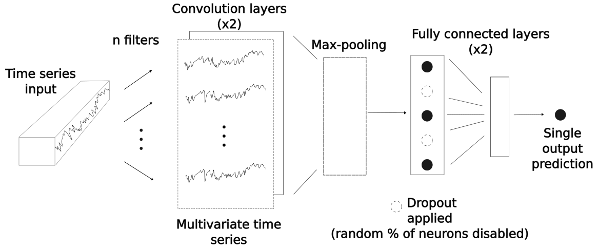
Figure 1Internal operations of a CNN. A set of filters is applied to the input time series in order to produce a multivariate time series in the convolutional layers. In the max-pooling layer (see main text), a feature vector is created that is further non-linearly transformed in the fully connected layers. In the fully connected layers, a dropout is applied for regularization purposes. A single output prediction is then produced, which is directly evaluated with its corresponding value in the target time series.
2.2 CNN-LSTMs
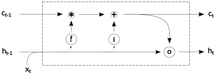
The architecture of the hybrid networks used in this study can be viewed as an array of two submodels: a CNN unit followed by a LSTM one. We first describe here LSTM generalities and functioning. This is followed by a description of the CNN-LSTM architecture implemented in this work. LSTMs are DL models are specifically designed to have memory cells (c) and hence have capacity for accumulating state information. In Fig. 2, an acyclic graph of a LSTM is presented. For each time step t, the input xt is processed and the computation of a hidden value ht is updated (being initialized as a vector of zeros in the first step). To control the memorizing process, LSTMs use “gating” mechanisms in their memory cells , where the role of each gate is to regulate the flow of information into and out of the cell. The first gate is the forget gate (introduced by Gers et al., 2000) and consists of a logistic sigmoid function σ and a pointwise multiplication operation. This gate controls which elements of the cell state vector ct−1 will be forgotten:
where Wf is a learnable weight matrix of the hidden state ht−1 and the input xt, and bf is a learnable bias vector. The resulting vector ft has values in the range (0, 1), where a value of 1 represents a complete information retention, and where 0 represents no information retention at all. In the second stage, it is decided what new information should be stored in the cell state. For this aim, the input gate is defined, where the values to be updated are specified:
where, in a similar way to the forget gate, Wi is the weight matrix, and bi is a bias vector. The resulting vector it contains information on which values will be updated, with values in the range (0, 1). This is followed by the computation of , a vector of new values – in the range (−1, 1) – that could be potentially added to the cell state:
where tanh is the hyperbolic tangent function, and Wc and bc are yet another pair of a learnable matrix and a bias vector, respectively. In the next step, we combine Eqs. (2)–(4) to update the cell state:
where × denotes element-wise multiplication. Finally, the output gate is defined. This gate controls the information that flows into the new hidden state ht and consists of a sigmoid function σ that filters which parts of the cell state will be passed on:
Then the new hidden state ht is updated:
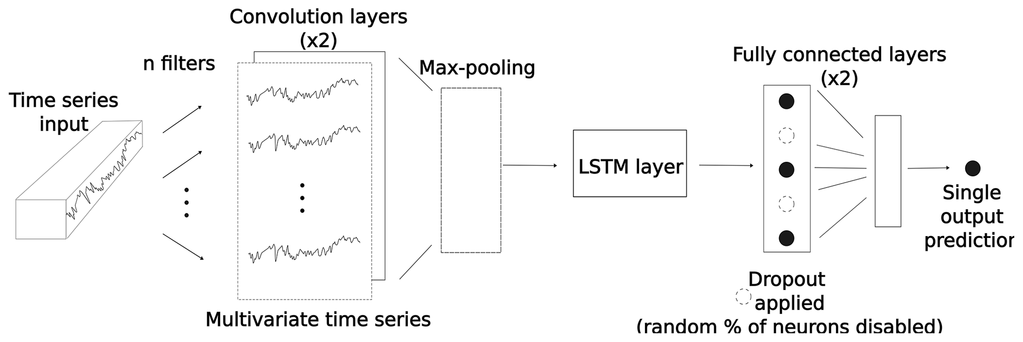
The described LSTM blocks can be either stacked in parallel to create deeper networks or used in tandem with other types of blocks to create hybrid networks, such as in CNN-LSTMs. While LSTMs were designed for sequence learning tasks (such as speech recognition), CNNs instead target spatial learning problems (such as object classification). The logic behind using hybrid CNN-LSTM networks is that the CNN component is used to extract deep features of the input data, while the LSTM component is used to learn how those features change with time. In other words, hybrid CNN-LSTM approaches are suitable for problems that have time-evolving multi-dimensional structures, a common property of coastal phenomena, where a myriad of processes encounter at diverse temporal and spatial scales.
Similarly to previously described CNN networks, the CNN unit in the implemented CNN-LSTMs consists of two convolutional layers followed by a max-pooling layer. The distilled feature vector obtained with the CNN unit is then used in the LSTM layer, where the LSTM layer allows the hybrid network to know what was predicted at the previous time step and accumulate information in the internal state (Fig. 3).
2.3 Calibration of deep learning models
DL models are trained to learn the mapping between a set of inputs and a set of outputs in an iterative cycle. During the training phase, output values are calculated within the network; these values are then compared to the “true” values with a given loss function in each step of the iteration cycle. The gradient of the loss function is then calculated explicitly with respect to the network's parameters. This is called backward propagation of errors or backpropagation for short; see Goodfellow et al. (2016) for a more detailed description. In this process, parameters and weights are adjusted to minimize the loss function in every iteration step.
Before training a network, a set of parameters must be defined; these are known as hyperparameters and control the learning process of the network. In contrast to weights and biases, whose final values are derived via training, hyperparameters are defined by the user. One example of this is the batch size, a hyperparameter that sets how many samples of the training data will be used in each iteration step before the network's parameters are updated. An epoch, defined as the period in which all the samples in the training dataset are used once to update the network, is another example of a hyperparameter.
A standard practice when calibrating DL models is to subdivide the data into three parts: the training (denoted train), development, and test sets. While the train set is used for the learning process of the network – where the weight and bias values are defined – the development set is used for evaluating the DL model while tuning model hyperparameters. Once the training and tuning processes are carried out, a final unbiased evaluation is then performed on the unseen test set.
2.4 Data
We here describe the set of inputs and outputs used to train, develop, and test the DL models. For the model inputs, we used wave and atmospheric drivers, while a shoreline time series was used as the target (or output) of our models. The study site is Tairua Beach, which is located in the Coromandel Peninsula, North Island of New Zealand (Fig. 4). Tairua Beach is a 1.2 km embayed beach with median sediment diameters (D50) of ∼0.3 mm, where the tidal range varies between 1.2–2 m. Shoreline position was captured with approximately daily observations over a period of 18 years (1999–2017) using a camera system at the south end of the beach. The image analysis and tidal correction applied to the images of the camera system are in line with previous studies (e.g. Guedes et al., 2011; Blossier et al., 2017; Montaño et al., 2020), where daily shoreline images with tidal levels between 0.45 and 0.55 m were selected in order to limit tidal influence. The images obtained were georectified and processed to extract shoreline time series. Then, in line with previous studies (e.g. Montaño et al., 2020, 2021), an alongshore-averaged cross-shore position was taken in order to obtain a single time series – the DL models' target. A weekly moving average is applied to the alongshore-averaged shoreline time series to filter noise affecting the small (less than daily) timescales, following Blossier et al. (2017) and Montaño et al. (2021).
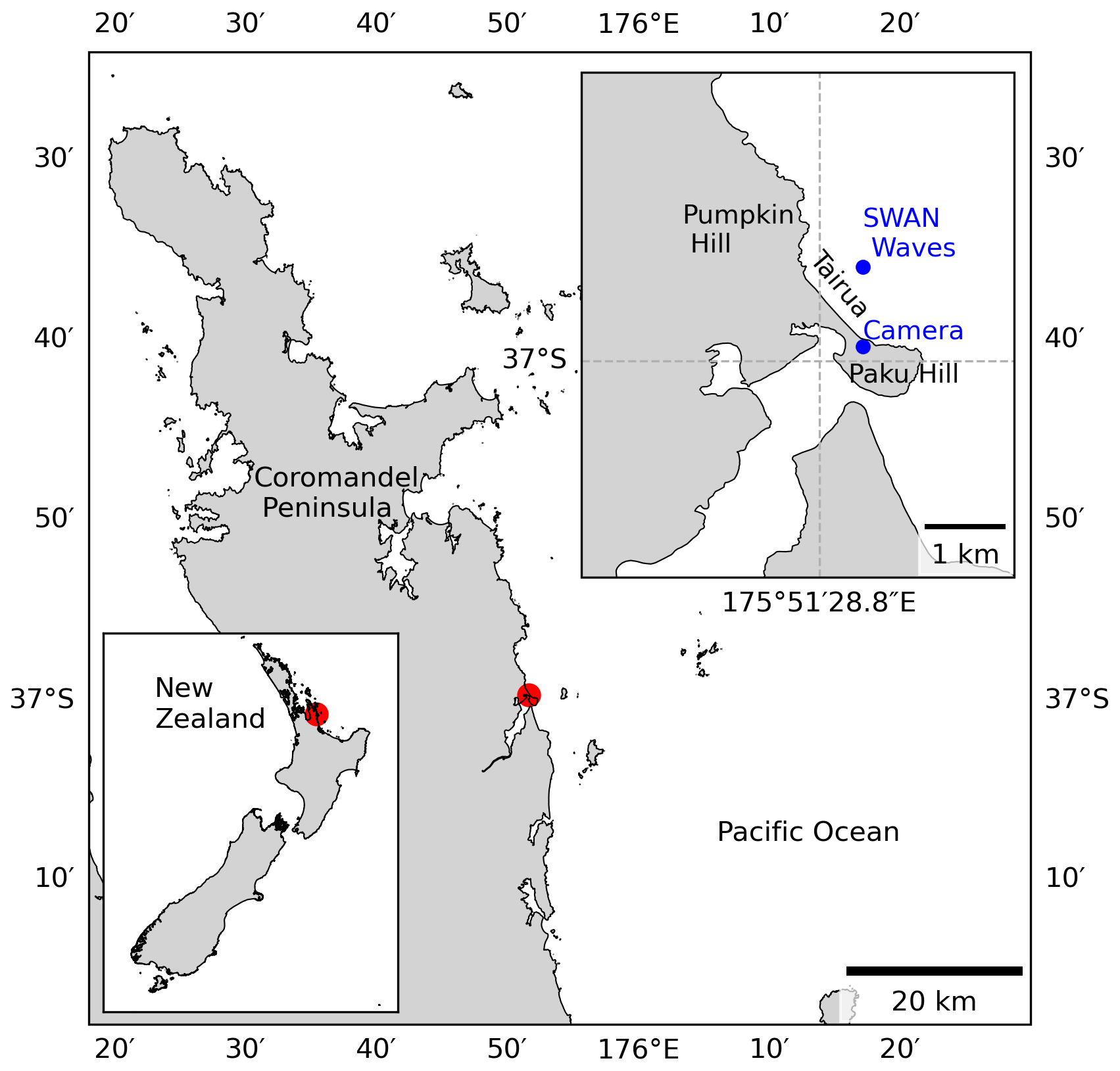
Figure 4Location of Tairua Beach on the Coromandel Peninsula in the North Island of New Zealand. Blue dots represent the installed camera system and the SWAN wave-bulk parameter location.
The traditional inputs for modelling shoreline position are wave-bulk parameters (i.e. significant wave height Hs, peak period Tp, and direction θ). We include these drivers by using the wave characteristics (at 10 m water depth) for daily-averaged time series in Montaño et al. (2020), obtained with the Simulating WAves Nearshore (SWAN; Booij et al., 1999) wave model (Fig. 5) and validated with in situ measurements in 8 m water depth. The data from the study site are freely available and have been used previously in other studies (e.g. Jaramillo et al., 2021; Vitousek et al., 2021; Lim et al., 2022).
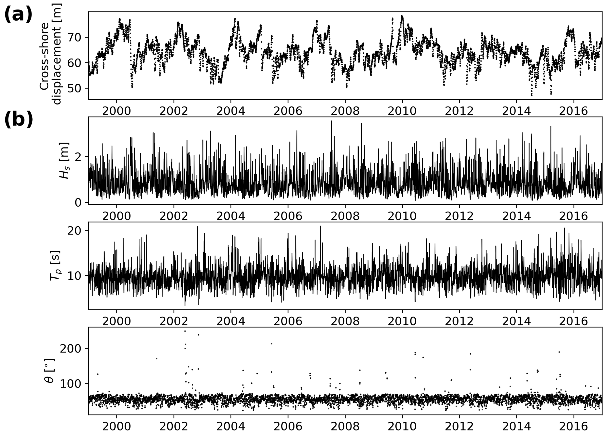
Figure 5Shoreline (target) time series, weekly averaged (a) and (b) daily wave-bulk parameters used as model inputs (Hs, Tp, θ) at Tairua Beach.
It has been shown that sea level pressure (SLP) can drive shoreline change by influencing wave climate in some study sites (e.g. Castelle et al., 2017; Harley et al., 2010). Although atmospheric drivers and wave parameters may contain similar information, atmospheric drivers may account for mean sea level fluctuations not retained in the wave parameters (Serafin and Ruggiero, 2014; Robinet et al., 2016), which in turn could improve model results. In order to account for the effects of atmospheric drivers at our study site, we included the first 10 principal components (PCs) derived from a principal component analysis of the SLP fields (carried out in Montaño et al., 2021) within the study site's wave genesis influence area. The influence area was identified using the ESTELA (Evaluating the Source and Travel time of the wave Energy reaching a Local Area) method (Pérez et al., 2014), which has been used for wave genesis characterization in other study sites (Camus et al., 2017; Cagigal et al., 2020; Silva et al., 2020; Lu et al., 2022).
To test the DL models, we use the time series previously presented in Montaño et al. (2021), generated with models SPADS (Montaño et al., 2021) and ShoreFor (Davidson et al., 2013); the coefficients for both SPADS and ShoreFor are determined in the models' calibration phase following optimization rules, no a priori information – besides wave model inputs and a shoreline target – is required.
The formulation of the equilibrium-based model ShoreFor (Davidson et al., 2013) used in Montaño et al. (2021) follows the modifications of Splinter et al. (2014), allowing for a general model with inter-site variability of model coefficients. The model contains two coefficients linked to wave-driven processes: (1) the memory decay parameter (ϕ) that describes the memory of a beach to previous wave conditions (notice this use of the concept “memory” is different than the one used in LSTMs) and (2) the rate parameter (c) that describes the sediment exchange efficiency between the beach face and surf zone. At Tairua Beach, the memory parameter ϕ has been found to be around 220 d (Montaño et al., 2021).
The data-driven model SPADS (Montaño et al., 2021) uses non-stationary time series decomposition methods to reconstruct shoreline oscillations at specific timescales (Sj) with statistically significant driver information (Y). Coefficients c that best fit the relation are optimized, where N=1, 2, …, i correspond to the number of drivers that are significant at the timescale considered, and the subindex j corresponds to the timescale of the shoreline being reconstructed.
2.5 Experimental design
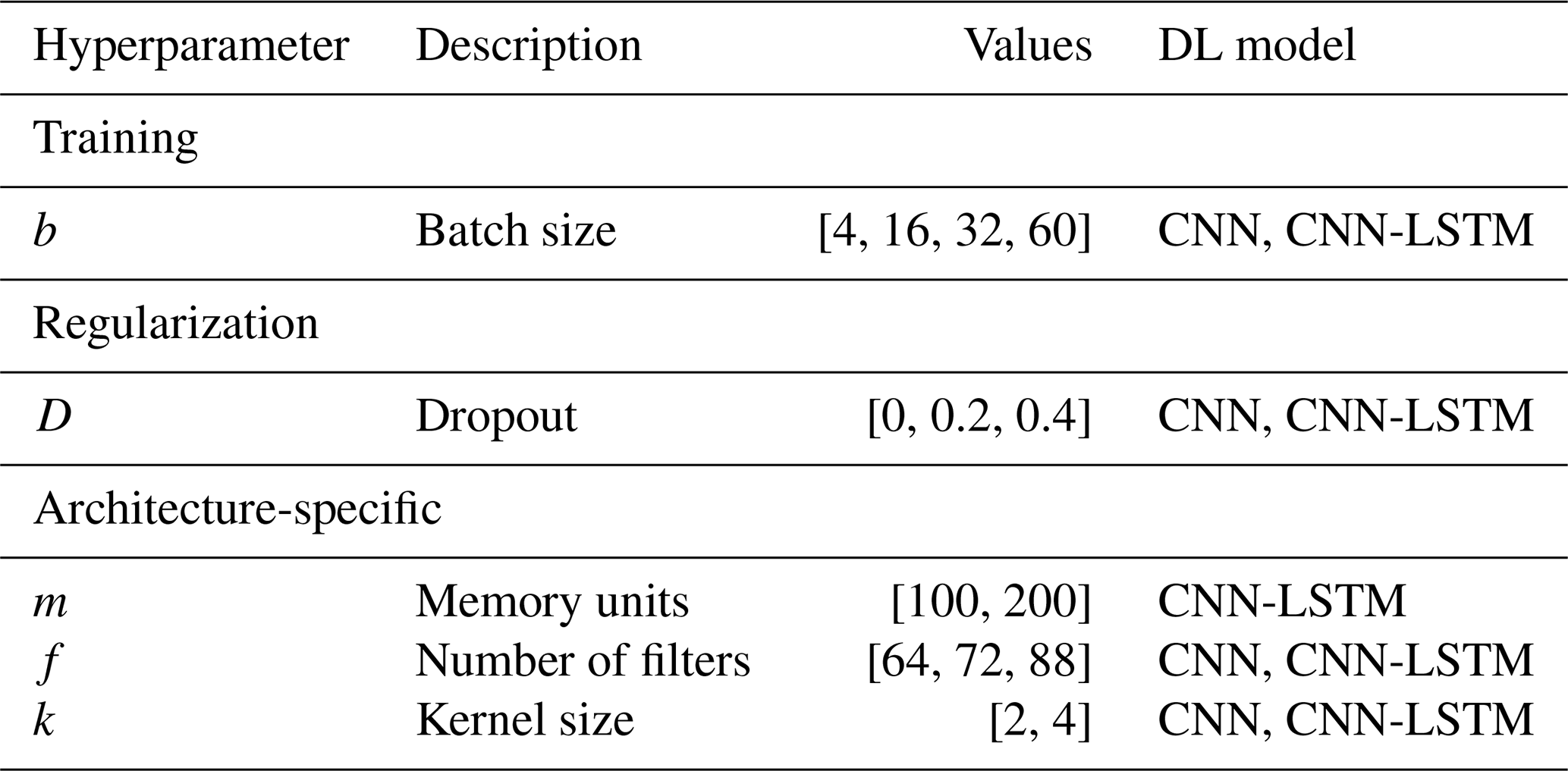
Finding well-performing model architectures and their hyperparameters is usually a hard and time-consuming process in DL (Larochelle et al., 2009). This process can also be non-intuitive, as model performance is highly sensitive to hyperparameter tuning. To shed light on the appropriate parameter space in which to train DL models when predicting shoreline time series, we designed a grid search to assess model unknowns. The focus is on exploring CNN and CNN-LSTM architectures, since LSTMs have been already implemented for our dataset (Montaño et al., 2020). In the grid search, different hyperparameters were varied according to each architecture (see Table 1). For the CNN, the number of filters and kernels in the convolutional layers was included in the grid search, while in the CNN-LSTM filters and kernels were varied in the convolutional layers and memory blocks were varied in the LSTM layers. For all networks, the batch size and the percentage of disabled neurons when applying dropout were varied in the grid search.
To train and evaluate the DL models, the data split was 14 years for the train set, 2 years for the development set, and 2 years for the test set. To carry out an efficient learning process, the inputs and outputs of the training data were normalized by removing the mean and dividing by the standard deviation. In the calibration process of DL models, it is common practice to calibrate a single network with varying random seeds. We instead used fixed realizations to allow for a straightforward and reproducible comparison with the benchmark results of ShoreFor (Davidson et al., 2013) and SPADS (Montaño et al., 2021), previously presented in Montaño et al. (2021).
Simultaneously, the designed grid search addressed the role of drivers and loss functions on network performance. With respect to the model drivers, the grid search explored wave-bulk parameters, atmospheric patterns, and the combination of these two as model inputs for DL models. These “driver” experiments were designed to gain insight into which shoreline change drivers might be relevant for the study site. In terms of the loss functions – essential components when training and evaluating DL models – the grid search addressed the use of the mean squared error (MSE) and the modified Mielke index (Duveiller et al., 2016). We use the modified Mielke index because it can be seen as a naturally bounded extension of the Pearson correlation coefficient and it also satisfies the conditions of being adimensional and symmetric (for more, see Duveiller et al., 2016). Mielke's index has previously shown useful for evaluating the ability of shoreline models to reproduce fast-scale oscillations (order of days) (Montaño et al., 2021) and can be written as (Duveiller et al., 2016)
where
Parameter n is the number of observed (x) and modelled (y) values, where and are the mean values and σx and σy are the standard deviations of the observed and simulated values, respectively; r is the Pearson correlation coefficient.
Taking into account the architectures, drivers, hyperparameters, and loss function variations in the grid search here implemented, around 1000 DL models were tested. Once the experiments were carried out, we further selected the best-performing models and performed averaging ensembles. The performance of the ensembles was analysed with Taylor diagrams (Taylor, 2001) and scatter plots. A graphical summary of the variables tested within the grid search and the metrics further used to evaluate the DL models can be seen in Fig. 6.
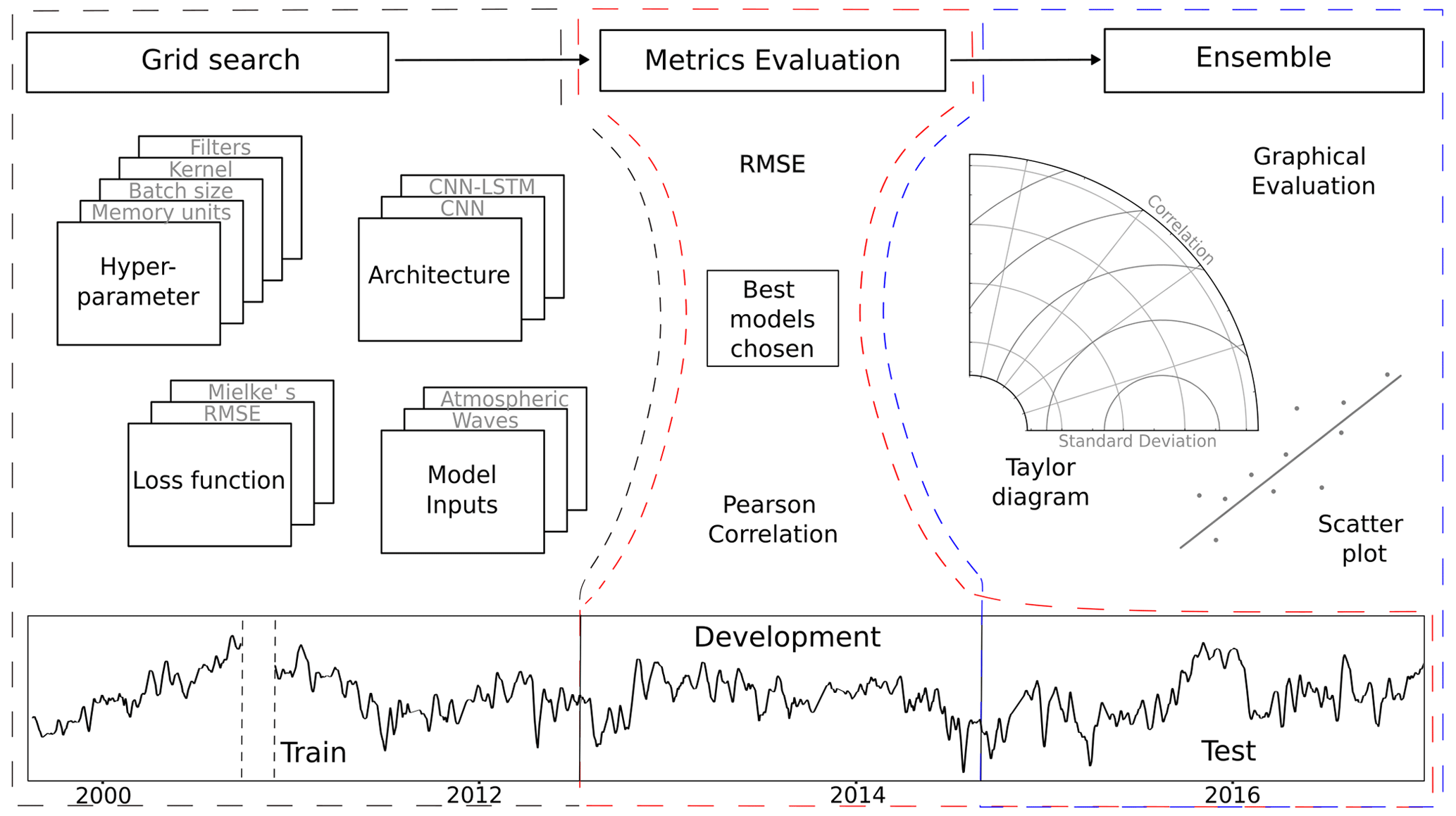
Figure 6Conceptual representation of the grid search (dashed black line), metrics evaluation (dashed red line) and ensemble (dashed blue line) processes for CNNs and CNN-LSTMs. For the grid search, the addressed model unknowns were the following: hyperparameter values, architectures, loss functions, and model inputs. Once the models were trained with 14 years of the data (train set), the models were evaluated based on their RMSE and Pearson correlations for both the development set (2 years) and the test set (2 years). Once the best-performing models were selected and an ensemble was formed, a further graphical evaluation was performed on the test set.
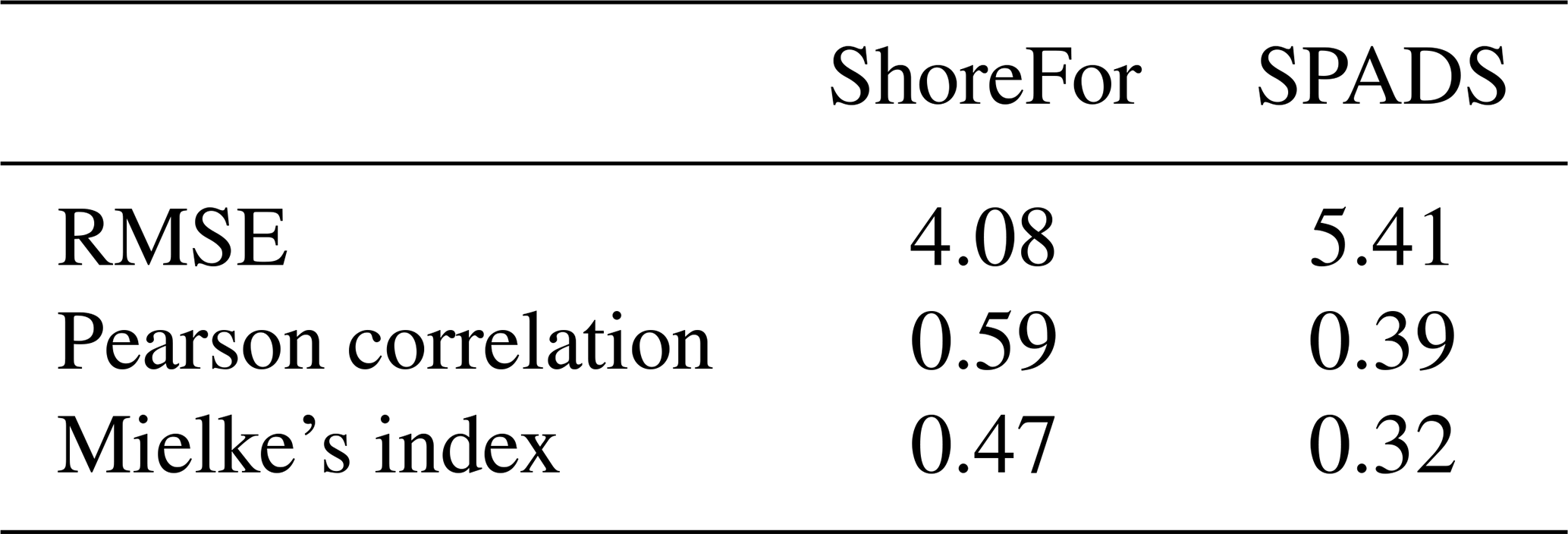
In order to visualize the performance of the multiple tests carried out with the grid search, we present a parallel coordinate plot (Fig. 7). Each subplot in Fig. 7 shows the performance of a specific set of numerical experiments, where each set is defined by the model architecture, combination of drivers, and loss function used. For all experiments, the values of the hyperparameters in Table 1 were used. An initial evaluation of model performance can also be seen in Fig. 7, where a Pearson threshold of ≥0.6 and a RMSE threshold of ≤5 m were set in both the development and test sets. These thresholds allowed for the detection of DL models that outperformed the benchmarks in terms of Pearson correlation while retaining a similar RMSE when compared to the best-performing benchmark (ShoreFor); see Table 2.
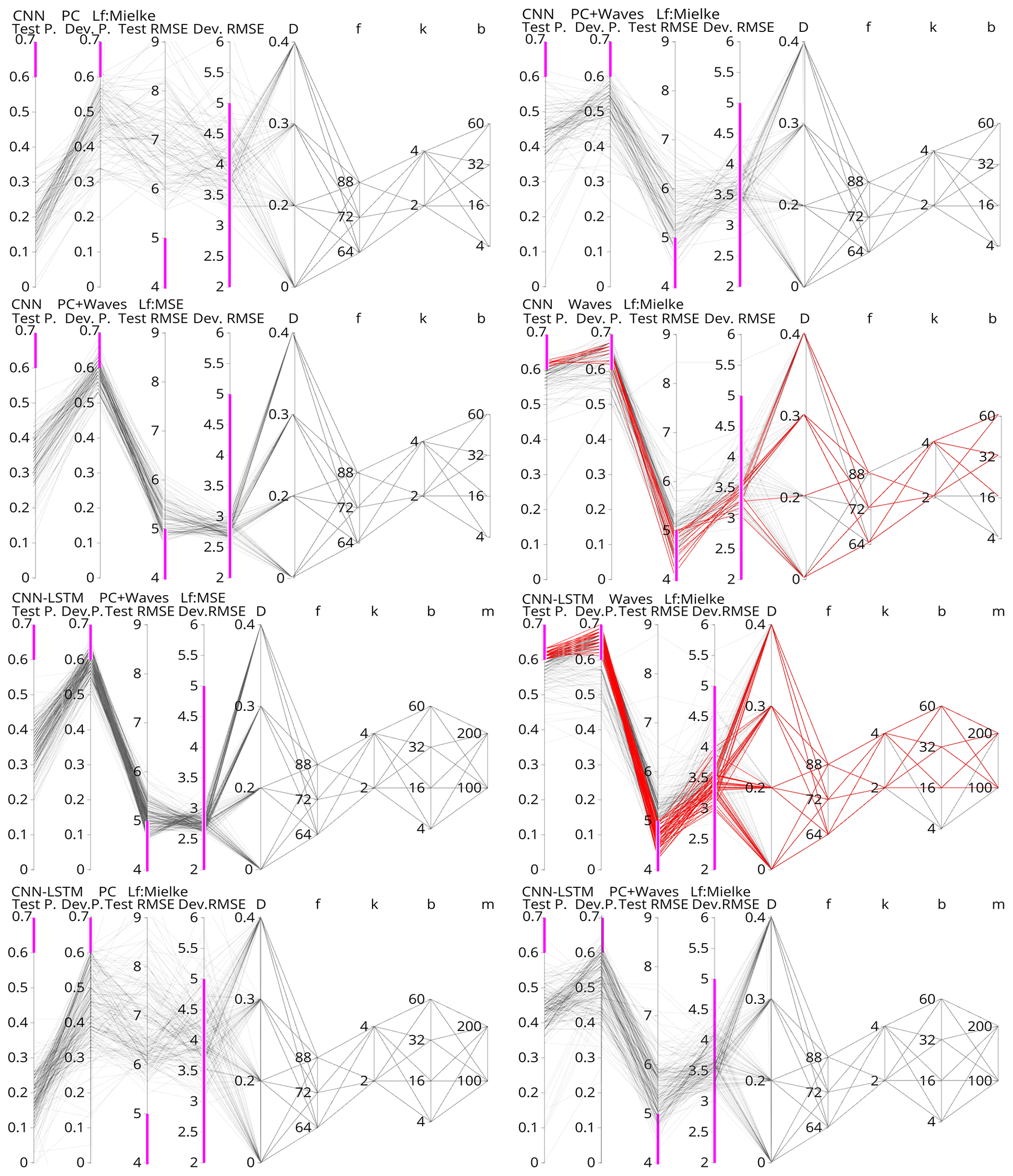
Figure 7Parallel coordinates of the numerical experiments carried out with CNN and CNN-LSTM networks. For each experiment, the first two attributes from left to right are the Pearson correlation obtained on the test and development set. The next two attributes are the RMSE on the test and development sets. The remaining five attributes are the hyperparameter values tested in the grid search: dropout percentage (D), number of filters (f), number of kernels (k), batch size (b), and memory units (m). Pink bars indicate the thresholds Pearson > 0.6 and MSE < 5, which indicate better or similar performance than the benchmarks. Models that simultaneously complied with these thresholds on the development and test sets are coloured red.
3.1 Driver experiments
As previously described, the grid search explored wave-bulk parameters, atmospheric patterns, and the combination of these two as model inputs for the DL models. These “driver” experiments were designed to gain insight into which shoreline change drivers might be relevant for the study site and period. Of all driver experiments, DL models trained solely with atmospheric patterns (represented by SLP PCs) obtained the lowest Pearson correlation coefficients (0.1–0.3) and highest RMSE values (>6 m) when compared with observations on the test dataset, while higher Pearson correlation values (0.3–0.5) and lower root-mean-square errors (RMSEs) (5–6 m) were obtained when SLP PCs along with wave-bulk parameters were used as model inputs (Fig. 7). The best-performing DL models were the ones trained solely with wave-bulk parameters, where the highest Pearson correlation values (>0.6) and lowest RMSEs (4–6 m) were obtained (Fig. 7).
The performance achieved with only-wave-trained DL models suggests that, among the two drivers tested, only wave inputs were relevant for shoreline change prediction at the study site. Although it has been discussed in previous work by Montaño et al. (2021) that differences between waves and SLP drivers could improve model performance when used together, our results indicate that the information contained in the SLP PCs does not add value to DL model predictions. This can also be seen in the apparently lower model performance when both drivers are used, an effect probably due to the well-known DL models' sensitivity to unnecessary data. Although SLP PCs were found to have little influence on shoreline change for the analysed timescale, these variables remain plausible model inputs, and in fact, the importance of atmospheric controls in shoreline change is becoming increasingly clear (e.g. Castelle et al., 2017; Vos et al., 2023).
3.2 Loss function and fine-tuning effects
As described in Sect. 2.5, the grid search also explored loss function and fine-tuning effects on previously selected architectures. The aim of the loss function trials was to explore the potential of Mielke's index for training DL models. In Fig. 7 we can see that in models that used both wave parameters and SLP PCs as inputs and MSE as the loss function, the average Pearson correlation obtained from the test set was ∼0.33 with maximum values of ∼0.55, while the RMSE minimum was ∼4.6 m. When Mielke's loss function was used instead, the average Pearson correlation obtained on the test set was ∼0.43, with maximum values of ∼0.63, while the RMSE minimum was ∼4.3 m. In other words, when Mielke's index was used as the loss function, higher correlations were obtained, although RMSE values remained similar when compared to MSE-trained networks.
The aim of exploring fine-tuning effects was to ensure robust results by obtaining populations of well-performing DL models. This was done by previously hand-picking good-performing network configurations and then performing a grid search on nearby values in the parameter space. In general, DL models proved sensitive to chosen drivers and loss function, while not much sensitivity to model hyperparameters was found, as expected. In Fig. 7 we can see 12 CNN models that met the thresholds of RMSE ≤5 m and Pearson ≥0.6 for both development and test sets, while 43 models that met those thresholds were obtained with the CNN-LSTM architecture.
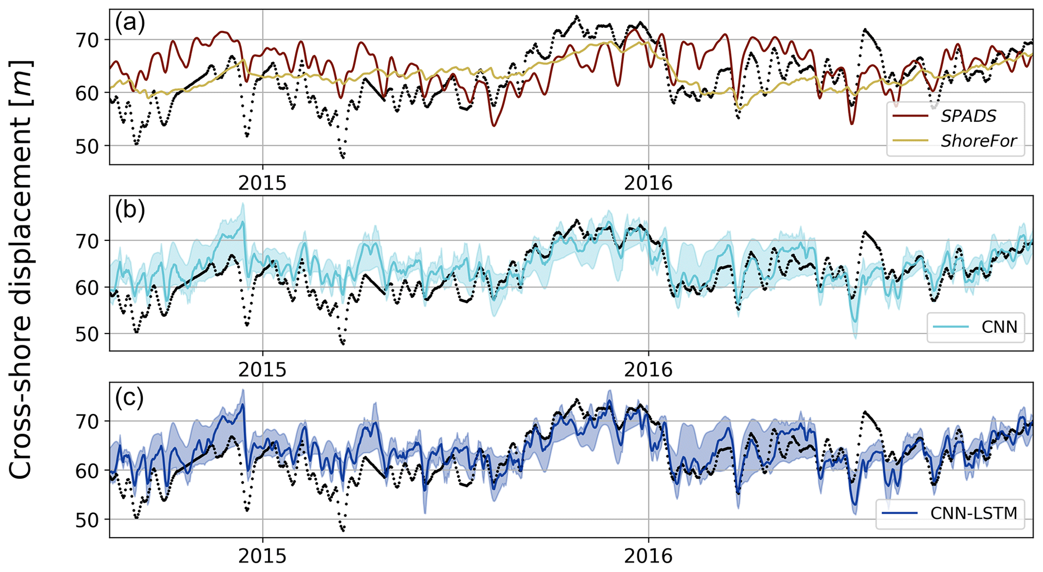
Figure 8Shoreline observations (in black) and predictions for the test set using ShoreFor and SPADS (a), CNN ensemble (b), and CNN-LSTM ensemble (c). For the CNN and CNN-LSTM ensembles, the min–max envelope is represented by shades.
3.3 Predictive capability
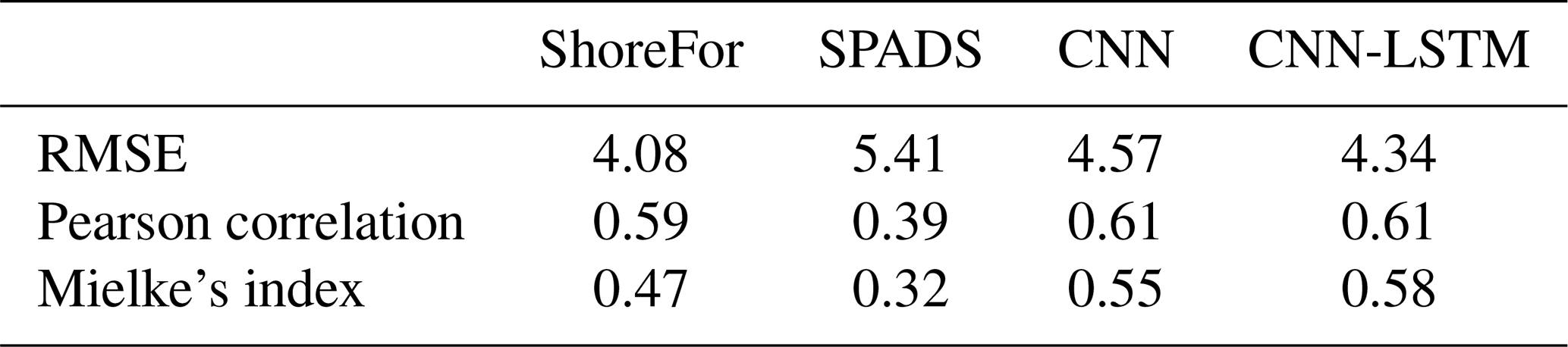
To compare the performance of CNNs and CNN-LSTMs with ShoreFor and SPADS, an averaging ensemble of the 10 best-performing DL models over CNN and CNN-LSTM populations was performed (Fig. 8). Following the results obtained in Sect. 3.1 and 3.2, the ensemble was performed over the networks of the only-wave experiments trained with Mielke's loss function. The first step taken to assess network performance was to calculate an absolute value error statistic (RMSE), along with normalized goodness-of-fit statistics (Pearson correlation and modified Mielke's index) on the test set. While the smallest RMSE was obtained with the ShoreFor model (4.08 m), the CNN-LSTM ensemble (4.34 m) and the CNN ensemble (4.57 m) closely followed, and SPADS obtained the highest value (5.41 m). On the other hand, the Pearson correlation/Mielke index was higher for the CNN-LSTM ensemble (), followed by the CNN ensemble (), ShoreFor (), and SPADS (); see Table 3.
In addition to traditional RMSE and Pearson metrics, we further analysed model performance by presenting graphical results. A Taylor diagram (Taylor, 2001) to further investigate model performance in time series variability and a density heat scatter plot to analyse model performance on data distribution are presented in Fig. 9. Both CNNs and CNN-LSTMs have the best locations in the metric space comprised by the Pearson correlation, centred RMSE, and standard deviation, with a standard deviation of ∼4.3 m for both network populations. SPADS is the second best in terms of standard deviation (3.5 m) predictability, while ShoreFor has the lowest time series standard deviation of all models (2.5 m). These results suggest that, out of the analysed models, DL models provide excellent performance as exhibited by a balance between standard deviation, Pearson correlation, and RMSE when reproducing the observations.
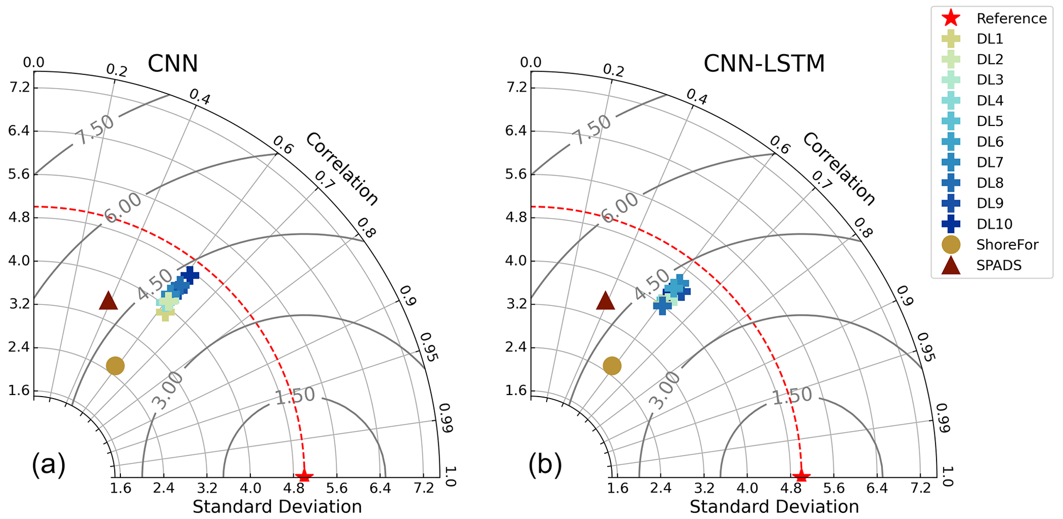
Figure 9Taylor diagrams on the test period. Performance of ShoreFor (brown), SPADS (green), and individual members of the CNN ensemble (a) and CNN-LSTM ensemble (b) compared with the observations (“ideal” performance in red).
Our results also indicate that appropriately trained DL models were the most accurate models when reproducing the distribution of observations (see Fig. 10). The location of points for each model in Fig. 10 showed that ShoreFor tended to reproduce only values near the mean, while SPADS had a more frequent overestimation of true values when compared to DL models. The absence of points in the low-value portion of all plots in Fig. 10 indicates that extreme erosion prediction remains a challenge. DL models' coverage of accretion/erosion is evident in Fig. 11, where the CNN-LSTM ensemble envelope was taken as a reference and covers 53.7 % of the observations with no time delay, with 62.1 % of the events allowing a ±1 d shift and 68.5 % of the events allowing a ±2 d shift.
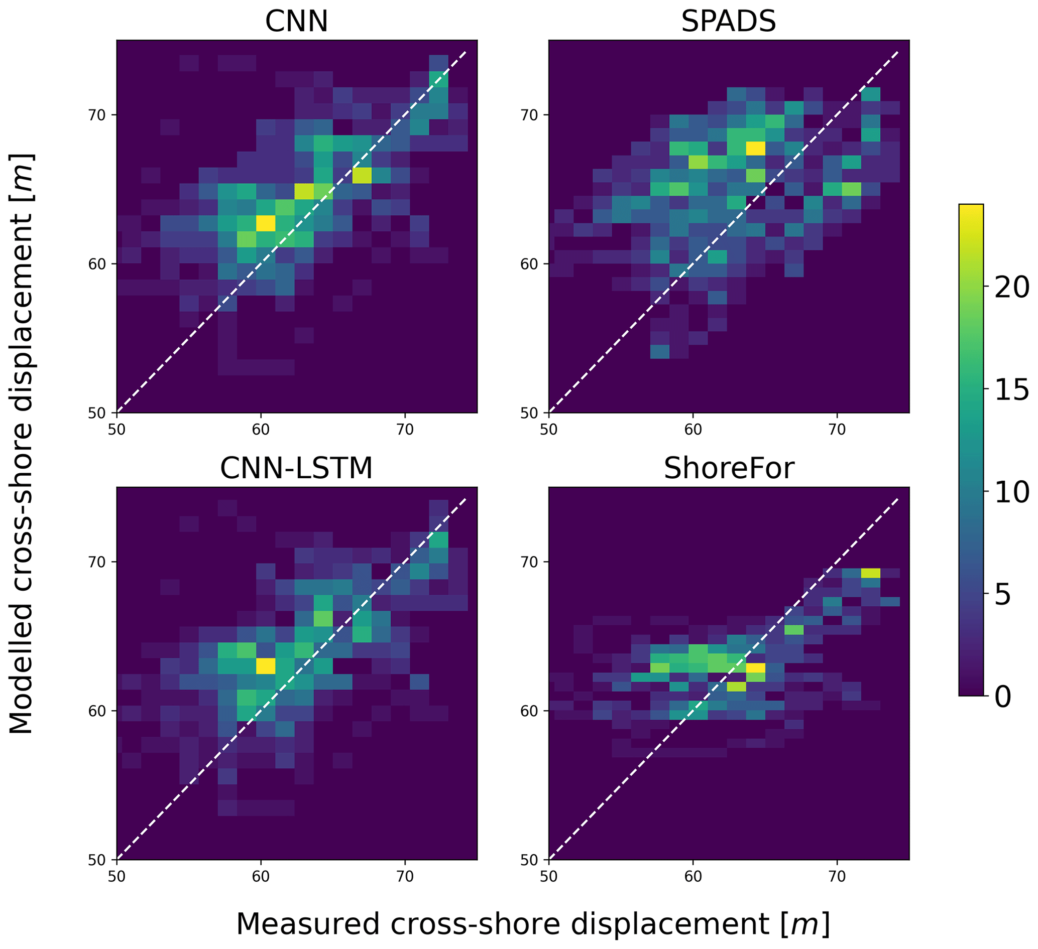
Figure 10Density heat scatter plot for the shoreline predictions of DL ensembles and benchmark models on the test period. The colour bar indicates the number of observations that fall within a given bin.
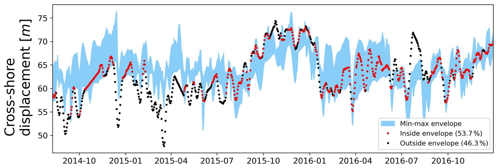
Figure 11Min–max envelope for the CNN-LSTM ensemble shoreline predictions (test period), marked in blue. Observations that fall inside the envelope (53.7 %) are marked in red, while observations that fall outside (46.3 %) are marked in black.
While there have been previous efforts to bring deep learning into shoreline time series prediction (e.g. Montaño et al., 2020; Pape et al., 2010), this work represents an extensive search and description of DL model configurations that proved effective for shoreline prediction. CNN and CNN-LSTM architectures were found to be effective, with the modified Mielke function (Duveiller et al., 2016) as an appropriate loss function for the training phase. Since shoreline evolution is known to have a strong autoregressive component, and as the LSTM unit can be seen as an element that retains detailed information on previous beach states, it would be expected that the CNN-LSTM architecture would outperform the CNN, an architecture lacking a memory unit – or an explicit memory beach parameter whatsoever. However, when comparing the performance between the CNN and CNN-LSTM, only minor differences were found (Figs. 9–11). Since the main aim of CNNs is to extract the representative features within data, one hypothesis to explain CNN competitive performance is that – despite being traditionally depicted as a strongly autoregressive process – shoreline evolution at the study site could alternatively be driven by a group of characteristic oscillations of the shoreline at different timescales. This in turn could suggest that knowing these characteristic oscillations could be sufficient for predicting shoreline evolution rather than only retaining detailed information on the immediate previous shoreline position. A similar result was found in Montaño et al. (2021), where the multiscale model SPADS with no explicit beach memory parameter was used.
The prediction of shoreline change has traditionally been made with process-based and equilibrium models (e.g. Davidson et al., 2013; Vitousek et al., 2017; Antolínez et al., 2019). But even though work is attempting to adapt shoreline models to reproduce isolated events under extreme conditions (e.g. McCall et al., 2010; Elsayed and Oumeraci, 2017), some of these models struggle to predict extreme and fast oscillations as noted in Montaño et al. (2020). As our results suggest, DL models could represent an alternative to more accurately reproduce the variability of shoreline change while simultaneously reproducing the average behaviour. In particular, DL models showed to be effective when reproducing the general distribution of observations when compared to benchmarks. Despite the above, extreme events remained a challenge to predict also for the DL approach. This could be due to the difficulty of gathering reliable data under extreme conditions (Sherwood et al., 2022) and therefore not having enough representative data of extreme events to train the models. A way this could be addressed could be by implementing a loss function in the training process that penalizes bad performance on outliers explicitly. Another possibility could be to generate synthetic data, a technique used in other fields, to compensate for the lack of data availability (e.g. Xu et al., 2020).
One of the concerns raised when using DL is its “black box”-like nature. To address this concern, an open research area in DL is the development of models that are constrained by physics principles (e.g. Wang et al., 2022). In addition, there are techniques that bring interpretability to DL models (e.g. gradient activation maps applied for coastal studies as in Rampal et al., 2022). While new models and techniques are being developed, DL models in their current state can also aid in giving insight into the study system when compared with traditional cross-shore morphodynamic models; here we showed that DL models trained with wave-bulk parameters as their only input were the most efficient when compared to traditional models, suggesting that wave parameters were the main drivers of shoreline change for the study site and test period. On the contrary, DL models trained with atmospheric drivers did not show a competitive performance, indicating that atmospheric-related drivers might have a small contribution at the study site, as reported for New Zealand in Vos et al. (2023), albeit for longer timescales than the ones analysed in this work.
DL is at an early stage of research in coastal science; while our understanding of these models deepens, we want to stress the importance of exploring DL through grid searching and ensemble modelling. The DL models developed here showed to be computationally efficient, enabling numerous trials that serve two purposes – first to find competitive configurations of DL models and second to provide a guideline on how to navigate the unknowns when using DL for the first time at a study site. When implementing our models for shoreline prediction, we addressed choosing among possible (i) model inputs, (ii) DL architectures, and (iii) model parameters.
- i.
A first layer of uncertainty lies on the chosen model inputs, where the use of grid searching allowed us to simultaneously test for combinations of atmospheric and wave inputs.
- ii.
Another layer of uncertainty is the chosen DL architecture; while previous work has been done with LSTMs in both coastal (Montaño et al., 2020) and other water sciences areas (Kratzert et al., 2018), many architectures with potential applications for earth science are yet to be studied (Reichstein et al., 2019). With the implemented grid search, we studied CNN and CNN-LSTMs, which are two types of DL models that showed competitive performance in shoreline prediction.
- iii.
The third and last unknown was parameter uncertainty, where values assigned to model parameters were varied in the grid-searching process. This allowed us to run different model versions, where an average ensemble of models was found to have competitive performance. Of the studies available for DL in shoreline prediction (e.g. Pape et al., 2010; Montaño et al., 2020), to our knowledge there is none that states the parameter values used. We here provide not only the parameter values used but also their uncertainty assessment through ensemble modelling, which could be valuable for future studies on DL models for shoreline prediction.
In previous studies, diverse metrics have been used to evaluate shoreline models' performance (e.g. Ibaceta et al., 2022; Jaramillo et al., 2020; Montaño et al., 2021), and although no consensus has been reached on a standard evaluation procedure, the current approach is to use a combination of absolute value error statistics, goodness-of-fit statistics, and graphical results, as done in other water science areas (e.g. Biondi et al., 2012). For this contribution, of particular interest was the assessment of the models' capability to reproduce the shoreline variability (which we consider to be captured by the standard deviation). Apart from an absolute value error statistic (RMSE) and a goodness-of-fit statistic (Mielke's index), we evaluated model ability to simulate observed variability with Taylor diagrams and scatter plots. The graphic results indicate that DL models outperform traditional models when simulating the variability of shoreline behaviour. The interpretation of our results could not have been achieved using only traditional metrics (i.e. RMSE, Pearson); hence, in this sense, we exhort shoreline modellers not only to continue to use a combination of metrics and graphical results but also to assure that shoreline models are being evaluated comprehensively.
This work investigated the potential of convolutional neural networks (CNNs) and CNN-LSTM (Long Short-Term Memory) networks to simulate shoreline evolution derived from camera system observations. The numerical experiments allowed us to explore the effects of varying model inputs, loss functions, and model hyperparameters in a systematic framework. The goal of this contribution was to show the potential of DL in shoreline change prediction; hence, a further exhaustive grid search for hyperparameters could be useful to find the best-performing DL model at the study site. The general findings of the experiments were the following:
-
Absolute-value-error and goodness-of-fit statistics in conjunction with graphical results indicate that DL models provide excellent performance when reproducing the observed shoreline position. In particular, the DL models implemented here were capable of reproducing the variability of shoreline evolution, outperforming established approaches.
-
DL can aid in deriving insight into which processes drive shoreline change. In this work, driver experiments indicate that shoreline change at the study site was wave-driven.
-
Model performance improved when using an extended version of the Pearson correlation coefficient as the loss function, hence demonstrating the benefit of exploring alternative metrics not only in the model evaluation stage but also in the training one.
Despite not having an explicit memory mechanism in their internal operations, CNNs performed similarly to CNN-LSTMs when simulating the observed shoreline change. Since CNN internal operations are designed to detect characteristic features of data, we hypothesize that this could be due to the nature of shoreline evolution at the site, a phenomenon that has been explained with oscillations at characteristic timescales in previous studies.
Since DL is particularly new to shoreline time series prediction, we find value in both the grid search and model ensembles here presented, since the former allowed for simultaneous tests on model unknowns, while the latter provided an uncertainty assessment of model parameter values. As a closing remark, we encourage future studies to make their data and model configurations publicly available to facilitate the implementation of DL shoreline models at multiple sites.
The alongshore-averaged cross-shore position time series, wave data, and code of the CNNs and CNN-LSTM models to reproduce the results shown here are publicly available on Zenodo at https://doi.org/10.5281/zenodo.10088350 (Gomez-de la Pena, 2023). The original shoreline data were curated by coauthor Jennifer Montaño and used in Montaño et al. (2021).
EGdlP conceived the methodology, analysed the results, and wrote the original manuscript. GC conceived the study, supervised the project, and contributed to reviewing. CW and JM contributed to reviewing.
The contact author has declared that none of the authors has any competing interests.
Publisher's note: Copernicus Publications remains neutral with regard to jurisdictional claims made in the text, published maps, institutional affiliations, or any other geographical representation in this paper. While Copernicus Publications makes every effort to include appropriate place names, the final responsibility lies with the authors.
The authors are grateful to Andres Payo, an anonymous referee, and associate editor Simon Mudd, whose comments improved the quality of the paper.
Eduardo Gomez-de la Peña is supported by The University of Auckland Doctoral Scholarship. This research has been supported by the MBIE project “Our Changing Coast” (grant no. E4349), secured by Giovanni Coco.
This paper was edited by Simon Mudd and reviewed by Andres Payo and one anonymous referee.
Antolínez, J. A., Méndez, F. J., Anderson, D., Ruggiero, P., and Kaminsky, G. M.: Predicting climate-driven coastlines with a simple and efficient multiscale model, J. Geophys. Res.-Earth, 124, 1596–1624, https://doi.org/10.1029/2018JF004790, 2019. a
Biondi, D., Freni, G., Iacobellis, V., Mascaro, G., and Montanari, A.: Validation of hydrological models: Conceptual basis, methodological approaches and a proposal for a code of practice, Phys. Chem. Earth Pt. a/b/c, 42–44, 70–76, https://doi.org/10.1016/j.pce.2011.07.037, 2012. a
Blossier, B., Bryan, K. R., Daly, C. J., and Winter, C.: Shore and bar cross-shore migration, rotation, and breathing processes at an embayed beach, J. Geophys. Res.-Earth, 122, 1745–1770, https://doi.org/10.1002/2017JF004227, 2017. a, b
Booij, N., Ris, R. C., and Holthuijsen, L. H.: A third-generation wave model for coastal regions. 1. Model description and validation, J. Geophys. Res., 104, 7649–7666, https://doi.org/10.1029/98JC02622, 1999. a
Buscombe, D. and Goldstein, E. B.: A reproducible and reusable pipeline for segmentation of geoscientific imagery, Earth Space Sci., 9, e2022EA002332, https://doi.org/10.1029/2022EA002332, 2022. a
Buscombe, D., Wernette, P., Fitzpatrick, S., Favela, J., Goldstein, E. B., and Enwright, N. M.: A 1.2 Billion Pixel Human-Labeled Dataset for Data-Driven Classification of Coastal Environments, Sci. Data, 10, 46, https://doi.org/10.1038/s41597-023-01929-2, 2023. a
Cagigal, L., Rueda, A., Anderson, D., Ruggiero, P., Merrifield, M. A., Montaño, J., Coco, G., and Méndez, F. J.: A multivariate, stochastic, climate-based wave emulator for shoreline change modelling, Ocean Model., 154, 101695, https://doi.org/10.1016/j.ocemod.2020.101695, 2020. a
Calkoen, F., Luijendijk, A., Rivero, C. R., Kras, E., and Baart, F.: Traditional vs. machine-learning methods for forecasting sandy shoreline evolution using historic satellite-derived shorelines, Remote Sens., 13, 934, https://doi.org/10.3390/rs13050934, 2021. a
Camus, P., Losada, I., Izaguirre, C., Espejo, A., Menéndez, M., and Pérez, J.: Statistical wave climate projections for coastal impact assessments, Earth's Future, 5, 918–933, https://doi.org/10.1002/2017EF000609, 2017. a
Castelle, B. and Harley, M.: Extreme events: Impact and recovery, in: Sandy Beach Morphodynamics, Elsevier, 533–556, https://doi.org/10.1016/B978-0-08-102927-5.00022-9, 2020. a
Castelle, B., Dodet, G., Masselink, G., and Scott, T.: A new climate index controlling winter wave activity along the Atlantic coast of Europe: The West Europe Pressure Anomaly, Geophys. Res. Lett., 44, 1384–1392, https://doi.org/10.1002/2016GL072379, 2017. a, b
Cooper, J. and McKenna, J.: Social justice in coastal erosion management: The temporal and spatial dimensions, Geoforum, 39, 294–306, https://doi.org/10.1016/j.geoforum.2007.06.007, 2008. a
Davidson, M. and Turner, I.: A behavioral template beach profile model for predicting seasonal to interannual shoreline evolution, J. Geophys. Res.-Earth, 114, F01020, https://doi.org/10.1029/2007JF000888, 2009. a
Davidson, M., Splinter, K., and Turner, I.: A simple equilibrium model for predicting shoreline change, Coast. Eng., 73, 191–202, https://doi.org/10.1016/j.coastaleng.2012.11.002, 2013. a, b, c, d, e, f, g
Duveiller, G., Fasbender, D., and Meroni, M.: Revisiting the concept of a symmetric index of agreement for continuous datasets, Sci. Rep., 6, 1–14, https://doi.org/10.1038/srep19401, 2016. a, b, c, d
Ellenson, A. N., Simmons, J. A., Wilson, G. W., Hesser, T. J., and Splinter, K. D.: Beach State Recognition Using Argus Imagery and Convolutional Neural Networks, Remote Sens., 12, 3953, https://doi.org/10.3390/rs12233953, 2020. a
Elsayed, S. M. and Oumeraci, H.: Effect of beach slope and grain-stabilization on coastal sediment transport: An attempt to overcome the erosion overestimation by XBeach, Coas. Eng., 121, 179–196, https://doi.org/10.1016/j.coastaleng.2016.12.009, 2017. a
Gers, F. A., Schmidhuber, J., and Cummins, F.: Learning to forget: Continual prediction with LSTM, Neural Comput., 12, 2451–2471, https://doi.org/10.1162/089976600300015015, 2000. a
Goldstein, E. B., Coco, G., and Plant, N. G.: A review of machine learning applications to coastal sediment transport and morphodynamics, Earth-Sci. Rev., 194, 97–108, https://doi.org/10.1016/j.earscirev.2019.04.022, 2019. a, b, c
Gomez-de la Pena, E.: eduardogomezdelapena/DL_shoreline_prediction: Code release with paper publication (Version 1), Zenodo [code and data set], https://doi.org/10.5281/zenodo.10088350, 2023. a
Goodfellow, I., Bengio, Y., and Courville, A.: Deep Learning, MIT Press, https://doi.org/10.1007/s10710-017-9314-z, 2016. a
Guedes, R. M. C., Bryan, K. R., Coco, G., and Holman, R. A.: The effects of tides on swash statistics on an intermediate beach, J. Geophys. Res.-Oceans, 116, C04008, https://doi.org/10.1029/2010JC006660, 2011. a
Gupta, M., Kodamana, H., and Sandeep, S.: Prediction of ENSO Beyond Spring Predictability Barrier Using Deep Convolutional LSTM Networks, IEEE Geosci. Remote Sens. Lett., 19, 1–5, https://doi.org/10.1109/LGRS.2020.3032353, 2022. a
Harley, M. D., Turner, I. L., Short, A. D., and Ranasinghe, R.: Interannual variability and controls of the Sydney wave climate, Int. J. Climatol., 30, 1322–1335, https://doi.org/10.1002/joc.1962, 2010. a
Hinton, G., Deng, L., Yu, D., Dahl, G. E., Mohamed, A.-r., Jaitly, N., Senior, A., Vanhoucke, V., Nguyen, P., and Sainath, T. N.: Deep neural networks for acoustic modelling in speech recognition: The shared views of four research groups, IEEE Sig. Process. Mag., 29, 82–97, https://doi.org/10.1109/MSP.2012.2205597, 2012a. a
Hinton, G. E., Srivastava, N., Krizhevsky, A., Sutskever, I., and Salakhutdinov, R. R.: Improving neural networks by preventing co-adaptation of feature detectors, arXiv [preprint], https://doi.org/10.48550/arXiv.1207.0580, 2012b. a
Hochreiter, S. and Schmidhuber, J.: Long Short-Term Memory, Neural Comput., 9, 1735–1780, https://doi.org/10.1162/neco.1997.9.8.1735, 1997. a
Ibaceta, R., Splinter, K. D., Harley, M. D., and Turner, I. L.: Improving multi-decadal coastal shoreline change predictions by including model parameter non-stationarity, Front. Mar. Sci., 9, 1012041, https://doi.org/10.3389/fmars.2022.1012041, 2022. a
Ismail Fawaz, H., Forestier, G., Weber, J., Idoumghar, L., and Muller, P.-A.: Deep learning for time series classification: a review, Data Min. Knowl. Discov., 33, 917–963, https://doi.org/10.1007/s10618-019-00619-1, 2019. a
Jaramillo, C., Jara, M. S., González, M., and Medina, R.: A shoreline evolution model considering the temporal variability of the beach profile sediment volume (sediment gain/loss), Coast. Eng., 156, 103612, https://doi.org/10.1016/j.coastaleng.2019.103612, 2020. a
Jaramillo, C., González, M., Medina, R., and Turki, I.: An equilibrium-based shoreline rotation model, Coast. Eng., 163, 103789, https://doi.org/10.1016/j.coastaleng.2020.103789, 2021. a
Kobayashi, N., Buck, . M., Payo, . A., and Johnson, B. D.: Berm and Dune Erosion during a Storm, J. Waterway Port Coast. Ocean Eng., 135, 1–10, https://doi.org/0.1061/(ASCE)0733-950X(2009)135:1(1), 2009. a
Kratzert, F., Klotz, D., Brenner, C., Schulz, K., and Herrnegger, M.: Rainfall–runoff modelling using long short-term memory (LSTM) networks, Hydrol. Earth Syst. Sci., 22, 6005–6022, https://doi.org/10.5194/hess-22-6005-2018, 2018. a
Krizhevsky, A., Sutskever, I., and Hinton, G. E.: Imagenet classification with deep convolutional neural networks, Adv. Neural Inform. Process. Syst., 25, 1097–1105, https://doi.org/10.1145/3065386, 2012. a, b
Larochelle, H., Bengio, Y., Louradour, J., and Lamblin, P.: Exploring strategies for training deep neural networks, J. Mach. Learn. Res., 10, 1–40, 2009. a
LeCun, Y., Boser, B., Denker, J., Henderson, D., Howard, R., Hubbard, W., and Jackel, L.: Handwritten digit recognition with a back-propagation network, Adv. Neural Inform. Process. Syst., 2, 396–404, 1989. a
LeCun, Y., Bengio, Y., and Hinton, G.: Deep learning, Nature, 521, 436–444, https://doi.org/10.1038/nature14539, 2015. a, b
Lees, T., Reece, S., Kratzert, F., Klotz, D., Gauch, M., De Bruijn, J., Kumar Sahu, R., Greve, P., Slater, L., and Dadson, S. J.: Hydrological concept formation inside long short-term memory (LSTM) networks, Hydrol. Earth Syst. Sci., 26, 3079–3101, https://doi.org/10.5194/hess-26-3079-2022, 2022. a
Lim, C., Kim, T.-K., and Lee, J.-L.: Evolution model of shoreline position on sandy, wave-dominated beaches, Geomorphology, 415, 108409, https://doi.org/10.1016/j.geomorph.2022.108409, 2022. a
Lu, W.-S., Tseng, C.-H., Hsiao, S.-C., Chiang, W.-S., and Hu, K.-C.: Future Projection for Wave Climate around Taiwan Using Weather-Type Statistical Downscaling Method, J. Mar. Sci. Eng., 10, 1823, https://doi.org/10.3390/jmse10121823, 2022. a
Luijendijk, A., Hagenaars, G., Ranasinghe, R., Baart, F., Donchyts, G., and Aarninkhof, S.: The state of the world's beaches, Sci. Rep., 8, 1–11, https://doi.org/10.1038/s41598-018-24630-6, 2018. a
Luijendijk, A., de Schipper, M., and Ranasinghe, R.: Morphodynamic acceleration techniques for multi-timescale predictions of complex sandy interventions, J. Mar. Sci. Eng., 7, 78, https://doi.org/10.3390/jmse7030078, 2019. a
McCall, R. T., De Vries, J. V. T., Plant, N., Van Dongeren, A., Roelvink, J., Thompson, D., and Reniers, A.: Two-dimensional time dependent hurricane overwash and erosion modelling at Santa Rosa Island, Coast. Eng., 57, 668–683, https://doi.org/10.1016/j.coastaleng.2010.02.006, 2010. a
McCarroll, R. J., Masselink, G., Valiente, N. G., Scott, T., Wiggins, M., Kirby, J.-A., and Davidson, M.: A rules-based shoreface translation and sediment budgeting tool for estimating coastal change: ShoreTrans, Mar. Geol., 435, 106466, https://doi.org/10.1016/j.margeo.2021.106466, 2021. a
Mentaschi, L., Vousdoukas, M. I., Pekel, J.-F., Voukouvalas, E., and Feyen, L.: Global long-term observations of coastal erosion and accretion, Sci. Rep., 8, 1–11, https://doi.org/10.1038/s41598-018-30904-w, 2018. a
Miller, J. K. and Dean, R. G.: A simple new shoreline change model, Coast. Eng., 51, 531–556, https://doi.org/10.1016/j.coastaleng.2004.05.006, 2004. a
Montaño, J., Coco, G., Antolínez, J. A., Beuzen, T., Bryan, K. R., Cagigal, L., Castelle, B., Davidson, M. A., Goldstein, E. B., and Ibaceta, R.: Blind testing of shoreline evolution models, Sci. Rep., 10, 1–10, https://doi.org/10.1038/s41598-020-59018-y, 2020. a, b, c, d, e, f, g, h, i, j, k
Montaño, J., Coco, G., Cagigal, L., Mendez, F., Rueda, A., Bryan, K. R., and Harley, M. D.: A Multiscale Approach to Shoreline Prediction, Geophys. Res. Lett., 48, e2020GL090587, https://doi.org/10.1029/2020GL090587, 2021. a, b, c, d, e, f, g, h, i, j, k, l, m, n, o, p, q, r
Murray, A. B.: Which Models Are Good (Enough), and When?, in: Treatise on Geomorphology, vol. 2, Elsevier Inc., 50–58, https://doi.org/10.1016/B978-0-12-374739-6.00027-0, 2013. a
Pape, L., Ruessink, B. G., Wiering, M. A., and Turner, I. L.: Recurrent neural network modelling of nearshore sandbar behavior, Neural Networks, 20, 509–518, https://doi.org/10.1016/j.neunet.2007.04.007, 2007. a
Pape, L., Kuriyama, Y., and Ruessink, B.: Models and scales for cross-shore sandbar migration, J. Geophys. Res.-Earth, 115, F03043, https://doi.org/10.1029/2009JF001644, 2010. a, b, c
Pérez, J., Méndez, F. J., Menéndez, M., and Losada, I. J.: ESTELA: a method for evaluating the source and travel time of the wave energy reaching a local area, Ocean Dynam., 64, 1181–1191, https://doi.org/10.1007/s10236-014-0740-7, 2014. a
Rampal, N., Shand, T., Wooler, A., and Rautenbach, C.: Interpretable Deep Learning Applied to Rip Current Detection and Localization, Remote Sens., 14, 6048, https://doi.org/10.3390/rs14236048, 2022. a
Ranasinghe, R.: Assessing climate change impacts on open sandy coasts: A review, Earth-Sci. Rev., 160, 320–332, https://doi.org/10.1016/j.earscirev.2016.07.011, 2016. a
Ranasinghe, R.: On the need for a new generation of coastal change models for the 21st century, Sci. Rep., 10, 2010, https://doi.org/10.1038/s41598-020-58376-x, 2020. a
Reichstein, M., Camps-Valls, G., Stevens, B., Jung, M., Denzler, J., and Carvalhais, N.: Deep learning and process understanding for data-driven Earth system science, Nature, 566, 195–204, https://doi.org/10.1038/s41586-019-0912-1, 2019. a, b, c, d
Robinet, A., Castelle, B., Idier, D., Le Cozannet, G., Déqué, M., and Charles, E.: Statistical modelling of interannual shoreline change driven by North Atlantic climate variability spanning 2000–2014 in the Bay of Biscay, Geo-Mar. Lett., 36, 479–490, https://doi.org/10.1007/s00367-016-0460-8, 2016. a
Roelvink, D., Reniers, A., van Dongeren, A., van Thiel de Vries, J., McCall, R., and Lescinski, J.: Modelling storm impacts on beaches, dunes and barrier islands, Coast. Eng., 56, 1133–1152, https://doi.org/10.1016/j.coastaleng.2009.08.006, 2009. a
Serafin, K. A. and Ruggiero, P.: Simulating extreme total water levels using a time-dependent, extreme value approach, J. Geophys. Res.-Oceans, 119, 6305–6329, https://doi.org/10.1002/2014JC010093, 2014. a
Sherwood, C. R., Van Dongeren, A., Doyle, J., Hegermiller, C. A., Hsu, T.-J., Kalra, T. S., Olabarrieta, M., Penko, A. M., Rafati, Y., and Roelvink, D.: modelling the morphodynamics of coastal responses to extreme events: what shape are we in?, Annu. Rev. Mar. Sci., 14, 457–492, https://doi.org/10.1146/annurev-marine-032221-090215, 2022. a
Shi, X., Chen, Z., Wang, H., Yeung, D.-Y., Wong, W.-K., and Woo, W.-C.: Convolutional LSTM network: A machine learning approach for precipitation nowcasting, in: Advances in Neural Information Processing Systems, vol. 28, edited by: Cortes, C., Lawrence, N., Lee, D., Sugiyama, M., and Garnett, R., Curran Associates, Inc., ISBN 9781510825024, 2015. a
Silva, A., Klein, A., Fetter-Filho, A., Hein, C. J., Méndez, F., Broggio, M., and Dalinghaus, C.: Climate-induced variability in South Atlantic wave direction over the past three millennia, Sci. Rep., 10, 18553, https://doi.org/10.1038/s41598-020-75265-5, 2020. a
Sit, M., Demiray, B. Z., Xiang, Z., Ewing, G. J., Sermet, Y., and Demir, I.: A comprehensive review of deep learning applications in hydrology and water resources, Water Sci. Technol., 82, 2635–2670, https://doi.org/10.2166/wst.2020.369, 2020. a
Splinter, K. D., Turner, I. L., Davidson, M. A., Barnard, P., Castelle, B., and Oltman-Shay, J.: A generalized equilibrium model for predicting daily to interannual shoreline response, J. Geophys. Res.-Earth, 119, 1936–1958, https://doi.org/10.1002/2014JF003106, 2014. a
Taylor, K. E.: Summarizing multiple aspects of model performance in a single diagram, J. Geophys. Res.-Atmos., 106, 7183–7192, https://doi.org/10.1029/2000JD900719, 2001. a, b
Toimil, A., Losada, I. J., Camus, P., and Díaz-Simal, P.: Managing coastal erosion under climate change at the regional scale, Coast. Eng., 128, 106–122, https://doi.org/10.1016/j.coastaleng.2017.08.004, 2017. a
Van, S. P., Le, H. M., Thanh, D. V., Dang, T. D., Loc, H. H., and Anh, D. T.: Deep learning convolutional neural network in rainfall–runoff modelling, J. Hydroinform., 22, 541–561, https://doi.org/10.2166/hydro.2020.095, 2020. a
Vitousek, S., Barnard, P. L., Limber, P., Erikson, L., and Cole, B.: A model integrating longshore and cross-shore processes for predicting long-term shoreline response to climate change, J. Geophys. Res.-Earth, 122, 782–806, https://doi.org/10.1002/2016JF004065, 2017. a, b, c
Vitousek, S., Cagigal, L., Montaño, J., Rueda, A., Mendez, F., Coco, G., and Barnard, P. L.: The application of ensemble wave forcing to quantify uncertainty of shoreline change predictions, J. Geophys. Res.-Earth, 126, e2019JF005506, https://doi.org/10.1029/2019JF005506, 2021. a
Vos, K., Harley, M. D., Turner, I. L., and Splinter, K. D.: Pacific shoreline erosion and accretion patterns controlled by El Niño/Southern Oscillation, Nat. Geosci., 16, 140–146, https://doi.org/10.1038/s41561-022-01117-8, 2023. a, b
Wang, N., Chen, Q., and Chen, Z.: Reconstruction of nearshore wave fields based on physics-informed neural networks, Coast. Eng., 176, 104167, https://doi.org/10.1016/j.coastaleng.2022.104167, 2022. a
Wright, L. D. and Short, A. D.: Morphodynamic variability of surf zones and beaches: a synthesis, Mar. Geol., 56, 93–118, https://doi.org/10.1016/0025-3227(84)90008-2, 1984. a
Xu, T., Coco, G., and Neale, M.: A predictive model of recreational water quality based on adaptive synthetic sampling algorithms and machine learning, Water Res., 177, 115788, https://doi.org/10.1016/j.watres.2020.115788, 2020. a
Yan, B., Zhang, Q.-H., and Wai, O. W.: Prediction of sand ripple geometry under waves using an artificial neural network, Comput. Geosci., 34, 1655–1664, https://doi.org/10.1016/j.cageo.2008.03.002, 2008. a
Yates, M. L., Guza, R. T., and O'reilly, W. C.: Equilibrium shoreline response: Observations and modelling, J. Geophys. Res, 114, 9014, https://doi.org/10.1029/2009JC005359, 2009. a, b
Yoon, H.-D., Cox, D. T., and Kim, M.: Prediction of time-dependent sediment suspension in the surf zone using artificial neural network, Coast. Eng., 71, 78–86, https://doi.org/10.1016/j.coastaleng.2012.08.005, 2013. a
Zhang, K., Geng, X., and Yan, X.-H.: Prediction of 3-D Ocean Temperature by Multilayer Convolutional LSTM, IEEE Geosci. Remote Sens. Lett., 17, 1303–1307, https://doi.org/10.1109/LGRS.2019.2947170, 2020. a