River incision, ¹⁰Be production and transport in a source-to-sink sediment system (Var catchment, SW Alps)

Detrital ¹⁰Be from continental river sands or submarine sediments has been extensively used to determine the average long-term denudation rates of terrestrial catchments, based on the assumption that the rate of cosmogenic nuclide production by the interaction of source rocks with cosmic radiation balances out the loss of these nuclides by surface denudation. However, the ¹⁰Be signal recorded in sediments may be affected at the source by the response time of mountainous catchments to high-frequency forcings. In addition, transient sediment storage in piedmonts, alluvial plains and lakes or near the coast may also induce a difference between the erosive signal and its record in the sedimentary sink. Consequently, a significant part of the signal recorded in shallow-water sediments can be lost, as deep marine sediments may simultaneously record a signal coming from newly eroded source rocks along with one coming from the destabilization of previously deposited sediments.

In this paper, we use the landscape evolution model Badlands to simulate erosion, deposition and detrital ¹⁰Be transfer from a source-to-sink sedimentary system (the Var River catchment, southern French Alps) over the last 100 kyr. We first compare model-based denudation rates with the ones that would be extracted from the ¹⁰Be record of local continental sediments (equivalent to river sands) and from sediments deposited offshore over time in order to examine if this record provides an accurate estimate of continental denudation rates. Then, we examine which conditions (precipitation rate, flexure, ice cover) satisfy published measured river incision rates and ¹⁰Be concentration in submarine sediments.

Our results, based on the Var catchment cosmic ray exposure dating and modelling indicate that, while river sands do accurately estimate the average denudation rate of continental catchments, this is much less the case for deep submarine sediments. We find that deep-sea sediments have a different and often much smoother ¹⁰Be signature than continental ones and record a significant time lag with respect to imposed precipitation rate changes, representing the geomorphological response of the margin. A model which allows us to fit both measured ¹⁰Be concentration in marine sediments and river incision rates on land involves an increase in precipitation rates from 0.3 to 0.7 m yr⁻¹ after 20 ka, suggesting more intense precipitation starting at the end of the Last Glacial Maximum.

1 Introduction

Sedimentary deposits are important archives of the tectonic and climatic history of continents: for instance, the geometry, grain size, mineralogy and geochemical signature of deposits are impacted by changes in environmental conditions (e.g. relative sea level changes and precipitation over geologic times as well as human activities during the Anthropocene) (Syvitski et al., 2022). Provided there are good enough estimates of the transfer function between these sedimentary records and their external forcing, they can be reliable tools for reconstructing climatic cycles, subsidence curves or monsoon onset, for instance (Bentley et al., 2016; Li et al., 2016; Liu et al., 2016; Wan et al., 2006). However, depending on the timescales considered, the signatures in submarine sediments of some of these external (i.e. climatic or tectonic) forcings affecting aerial catchments depend on a myriad of processes which still remain difficult to extract from the deep-sea record. To this end, one would need to evaluate not only how the eroded source responds to specific forcing but also for how long and where detrital sediments are temporarily stored and when they are re-injected into the system and eventually reach their sink.

Concerning the sediment source, mountainous catchments may not be very sensitive to high-frequency forcing, and the response time of these catchments may already affect the signal recorded in locally produced sediments (e.g. Armitage et al., 2013; Godard and Tucker, 2021; Goren, 2016; Jerolmack and Paola, 2010). Second, transient sediment storage in piedmonts, alluvial plains and lakes or near the coast may induce a large time lag between the external signal and its record in the sedimentary sink (e.g. Blöthe and Korup, 2013; Clift and Giosan, 2014; Malatesta et al., 2018; Phillips and Slattery, 2006; Romans et al., 2016). Depending on considered timescales, the erosive signal itself can be completely buffered by this process (see a complete review in Romans et al., 2016). Finally, submarine sediments can be reworked by gravitational processes, especially during sea level falls (Phillips and Slattery, 2006). As a consequence, a significant part of the signal recorded in shallow-water sediments can be lost, whereas deep marine sediments may simultaneously record a signal coming from newly eroded source rocks and another one coming from the destabilization of previously deposited sediments. In addition, relative sea level variations may affect the connectivity between aerial rivers and submarine canyons, therefore, from time to time, limiting the efficiency of sediment transport in the offshore domain (Fryirs et al., 2007).

Detrital terrestrial cosmogenic nuclide (TCN; mostly ¹⁰Be) concentrations from continental river sands or submarine sediments have been extensively used to determine the average long-term denudation rates of aerial catchments, provided enough quartz-bearing rocks outcrop at the surface to give a representative sampling of the whole catchment denudation (e.g. Bierman and Steig, 1996; von Blanckenburg, 2005; Lupker et al., 2012; Mandal et al., 2015; Siame et al., 2011; Vanacker et al., 2007). Denudation rate estimates from ¹⁰Be concentration in quartz-rich sediments are often based on the assumption that the rate of TCN production by the interaction of source rocks with cosmic radiation balances out the loss of these elements by surface denudation (Lal, 1991). Denudation rates can vary in time and space, which puts this steady-state assumption into question and may lead to under- or overestimates of the true denudation rates (Bierman and Steig, 1996). The abundance of the target mineral (i.e. quartz in the case of ¹⁰Be) in surface rocks may also vary and has to be taken into account in order to correctly estimate the total production rate of a given catchment (Bierman and Steig, 1996; Safran et al., 2005; Carretier et al., 2015).

Moreover, sediments can be seen as an amalgamation of individual grains of different sizes and with different histories: alluvial terraces contain various clasts, the TCN concentration of which is linked to the erosion rate of their catchment (inheritance) and to posterior TCN production (Repka et al., 1997). The distribution of TCN concentration in individual grains depends on the geomorphic processes acting at the source and on the post-erosion TCN production (Codilean et al., 2010). Numerical models of individual grains' journeys have shown that some grains may have very long residence times in the piedmont (i.e. of the order of 100 kyr) and may therefore be exported to their final depositional area long after they have been produced by bedrock erosion (Carretier et al., 2020). Landslides may also significantly affect denudation rate estimates from TCN if the catchment area is small (Yanites et al., 2009). Hence, understanding how detrital ¹⁰Be concentrations recorded in submarine sedimentological archives reflect denudation rates at the time of their deposition requires quantifying the following: (i) how, how fast and where ¹⁰Be is produced; (ii) how ¹⁰Be concentration in the sediments produced is representative of average catchment denudation rates at any given spatiotemporal scale (Zerathe et al., 2022); and (iii) how long it has taken for sediments, once they are produced, to reach the sedimentary sink where they have potentially been sampled.

In this paper, we adapt the surface process model Badlands (Salles, 2016) to simulate erosion, deposition and detrital ¹⁰Be transfer from a source-to-sink sediment system (the Var River catchment, southern French Alps, and its marine depositional system in the Mediterranean Sea) over the last 100 kyr. We first compare simulated denudation rates with the ones that would be inferred from the ¹⁰Be concentration of continental sediments (equivalent to river sands) or sediments deposited offshore at each time step in order to assess at which timescales the steady-state assumption is valid and whether ¹⁰Be record in detrital sediments provides an accurate estimate of continental denudation rates. Then, we examine which conditions (precipitation rate, flexure, ice cover) satisfy published river incision rates (Cardinal et al., 2022; Petit et al., 2019; Rolland et al., 2017, 2020; Saillard et al., 2014) and ¹⁰Be concentration in marine sediments (named hereafter ¹⁰Be_MS) in this particular, small-scale source-to-sink system (Mariotti et al., 2021).

2 Geomorphological and geological setting

The Var catchment in the southern French Alps is ideally suited to constrain source-to-sink processes: it is a relatively small catchment (∼2800 km²), which encompasses some of the high-altitude (∼3000 m) summits of the Alpine Mercantour crystalline massif (Fig. 1). The Var River has three main large tributaries: the Tinée and Vésubie rivers, the headwaters of which are in the crystalline massif, and the Estéron River, which flows only across the overlying Mesozoic to Cenozoic sedimentary sequence. The hydrologic regime of the Var River, dominated by flash floods, is responsible for frequent hyperpycnal flows in the submarine domain (Mulder et al., 1998). The continental floodplain and shelf at the mouth of the Var River are very narrow, and most detrital sediments are deposited offshore at the foot of the Ligurian margin (Mediterranean Sea) at depths below −2000 m. The average annual discharge at the mouth of the Var River is ∼50 m³ s⁻¹, but it can reach more than 500 m³ s⁻¹ during floods (Mulder et al., 1998). According to Mulder et al. (1998) and Syvitski et al. (2000), the suspended sediment load C_s can be obtained from the following expression:

$$\begin{array}{}\text{(1)}& C_{\mathrm{s}}=a{Q}_{\mathrm{w}}{}^b,\end{array}$$

where parameters a [M L⁻³] and b relate the sediment concentration C_s [M L⁻³] to mean discharge Q_w [L³ T⁻¹] at the river mouth, and have been estimated to be $\sim \mathrm{7.7}\times {\mathrm{10}}^{-\mathrm{4}}$ and ∼1.65 for the Var River, respectively, from direct measurements of suspended sediment concentration and water discharge (Mulder et al., 1998). Modern average denudation rate estimates of the Var River catchment from ¹⁰Be measurements in fluvial sediments range between 0.1 and 0.8 mm yr⁻¹ (Mariotti et al., 2019). Two other coastal rivers flow east of the Var catchment: the Paillon and Roya rivers, with much smaller drainage areas (258 and 601 km², respectively).

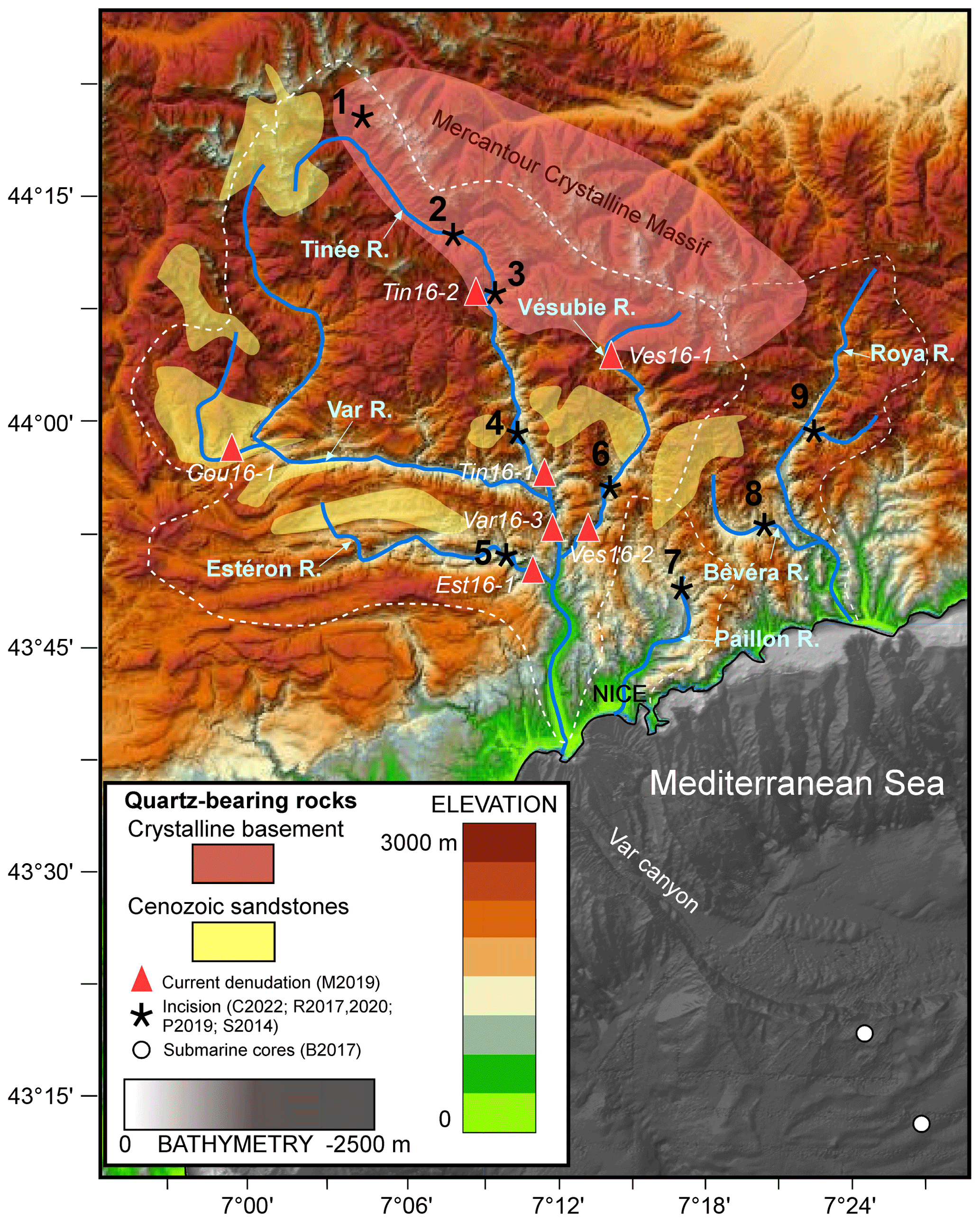
Figure 1 Topographic and bathymetric map and schematic outline of main quartz-bearing rock outcrops of the study area (transparent red and yellow patches). Dashed white lines indicate the contours of the Var, Paillon and Roya river catchments. Stars, open dots and triangles indicate the location of data constraints provided by the following: surface exposure dating of river-polished surfaces (after Saillard et al., 2014 – S2014; Rolland et al., 2017, 2020 – R2017 and R2020; Petit et al., 2019 – P2019; Cardinal et al., 2022 – C2022), geochemical analyses of submarine sediments (Bonneau et al., 2017 – B2017) and detrital ¹⁰Be in river sands (Mariotti et al., 2019 – M2019). For river-polished surfaces, the numbers refer to the following sites: 1 – Salso Moreno; 2 – Isola; 3 – Saint-Sauveur; 4 – lower Tinée; 5 – Estéron; 6 – Vésubie; 7 – Paillon; 8 – Bevera; 9 – Roya. Italic expressions refer to sample names in Mariotti et al. (2019).

A previously published paper presented detailed sedimentological and geochemical analyses of sediment cores in the sedimentary ridge located at the outlet of the Var submarine canyon (Bonneau et al., 2017) (Fig. 1). These analyses revealed a larger frequency of turbidite flows and slightly larger epsilon-Nd (ϵ_Nd) values during the Last Glacial Maximum (LGM), which is interpreted as reflecting more intense erosion, especially in the crystalline massif, and larger sediment production during glacial periods. In these cores, ¹⁰Be_MS varies between 2×10⁴ and 7×10⁴ at. g⁻¹ (atoms per gram of quartz), which corresponds to average denudation rates of 0.2 to 0.5 mm yr⁻¹ between 70 and 4 ka (Mariotti et al., 2021). On land, cosmic ray exposure (CRE) ages of polished river cliffs have revealed fast incision rates of ∼0.5 to 2 mm yr⁻¹ during the Late Pleistocene at most sites of the Var catchment and in the Bevera River (Cardinal et al., 2022; Petit et al., 2019; Rolland et al., 2017; Saillard et al., 2014). River gorges located at high altitudes in the Mercantour massif (Sites 1 and 2 in Fig. 1; red and brown dots in Fig. 2) show very fast incision (up to 4 mm yr⁻¹) starting after the Younger Dryas (YD), which can be ascribed to a transient response of formerly glaciated valleys. Most of the lower-altitude river gorges (Sites 3, 4, 5, 6 and 8 in Fig. 1; orange, yellow and green dots in Fig. 2) start to be incised around 20 ka (i.e. close to the LGM). Two other sites (7 and 9 in Fig. 1; cyan and blue dots in Fig. 2) show much lower incision rates (<0.5 mm yr⁻¹) extending from 0 to 80 ka.

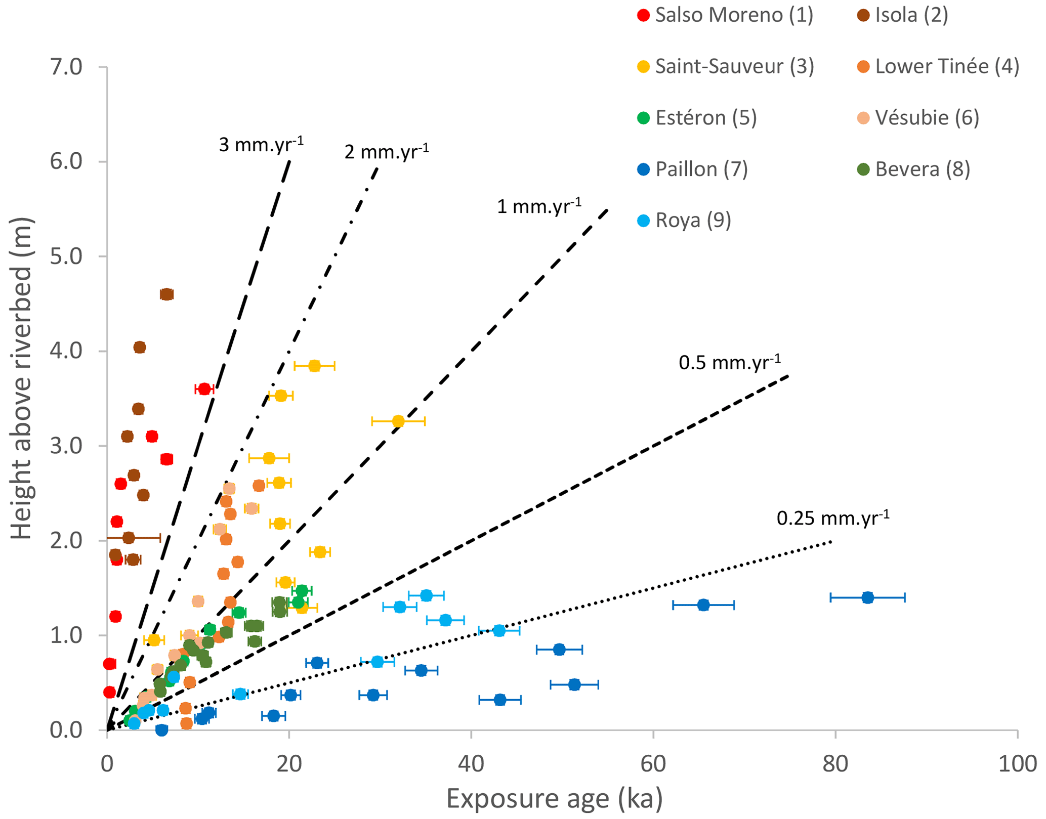
Figure 2 Altitude above the riverbed vs. cosmic ray exposure (CRE) ages and corresponding error bars in samples of river-polished surfaces of the Var, Roya and Paillon catchments (Cardinal et al., 2022; Rolland et al., 2017, 2020; Petit et al., 2019; Saillard et al., 2014). See location of the sites in Fig. 1. Dashed lines indicate constant incision rate curves for comparison.

Previously published interpretations of these data have suggested that rivers with sources in previously glaciated areas (Tinée, Vésubie) incised faster during and after the LGM not only because of increasing precipitation but also because of the massive release of glacier meltwaters and stored sediments occurring at that time (e.g. Saillard et al., 2014; Rolland et al., 2020). More recently, Cardinal et al. (2022) have pointed out a complex response of river systems of the SW French Alps to deglaciations, depending on their connection with glaciated areas and on the presence of lithological knickpoints.

To summarize, river incision data suggest the following: (1) transient and rapid incision following the Younger Dryas in high-altitude areas; (2) steady, fast incision rates of ∼1 mm yr⁻¹ for the last 15–20 kyr at almost all other points; and (3) lower incision rates of ∼0.2 to 0.5 mm yr⁻¹ in the Paillon and Roya rivers, east of the Var catchment. In all catchments, it appears that data points in the last ∼20 kyr range along slopes that define larger incision rates (sometimes by 1 order of magnitude) than average catchment denudation rates estimated from detrital ¹⁰Be in river sands or marine sediments (Mariotti et al., 2019, 2021). This is not necessarily contradictory, as incision is a local phenomenon compared to the average catchment surface denudation. In particular, gorges where fast incision occurs can typically induce a transient decoupling from the catchment base level for the surrounding hillslopes (Reinhardt et al., 2007). However, there is a fundamental difference in the interpretation of river incision rates and ¹⁰Be_MS from deep marine sediments: while gorge bedrock surface exposure ages in the last 20 kyr define high incision rates, suggesting that the post-LGM period was characterized by enhanced incision and gorge entrenchment, the geochemical signature of marine sediments is interpreted (Bonneau et al., 2017; Mariotti et al., 2021) as reflecting more intense erosion during the glacial episodes than during deglaciations.

3 Methods

3.1 Landscape evolution model

We use the landscape evolution model (LEM) Badlands (Salles, 2016) to simulate erosion and deposition on an TIN topographic grid under various tectonic (uplift) and climatic (precipitation, hillslope processes) time and space parameters. River incision is simulated using the stream power law (SPL) (Whipple and Tucker, 1999):

$$\begin{array}{}\text{(2)}& \mathit{\epsilon }=K{\left(\stackrel{\mathrm{‾}}{P}\cdot A\right)}^m{S}^n,\end{array}$$

where ε is the erosion rate [L T⁻¹], K is a dimensional coefficient that describes the erosional efficiency [L^1–2m T⁻¹], A is the drainage area [L²], $\stackrel{\mathrm{‾}}{P}$ is the spatial and temporal variation in precipitation rate P relative to a mean precipitation rate P₀ (1 m yr⁻¹; the product being used as a proxy for the discharge), S is the channel slope, and m and n are positive exponents. An $m/n$ value close to 0.5 was previously estimated in the Var and Vésubie catchments (Saillard et al., 2014; Petit et al., 2017), so in all models, we chose to set  m and n to the classically used values of 0.5 and 1, respectively, and to tune the K value in order to fit measured incision rates. Hillslope processes on land and short-distance sediment transport at sea can be simulated by a linear diffusion law:

$$\begin{array}{}\text{(3)}& {\displaystyle \frac{\mathrm{d}h}{\mathrm{d}t}}=K_{\mathrm{D}}{\mathrm{\nabla }}^{\mathrm{2}}h,\end{array}$$

where $\mathrm{d}h/\mathrm{d}t$ is the altitude change due to diffusive processes [L T⁻¹], h is the altitude [L] and K_D is the hillslope diffusion coefficient [L² T⁻¹], which can vary between the continental and marine domains. We fix the diffusion coefficient to low values (0 to 0.025 m² yr⁻¹) both on land and at sea in order to ensure that any observed smoothing effect on the ¹⁰Be record in deposited sediments is not due to diffusive processes (Table 2). For the same reason, we do not consider non-linear diffusion components. For river systems, we use the detachment-limited law (Eq. 2), but we impose sediment deposition either when the channel slope falls below a given threshold (alluvial plain deposition; see Table 3) or when the rivers reach their base level or an endorheic depression. In these cases, available sediment fluxes carried by rivers are used to compute the volume of sediments to deposit. If transported sediment fluxes, when deposited, are insufficient to fill the depression or to reach the prescribed channel slope threshold, all sediments would be deposited and the outgoing river sediment concentration would be zero. If, on the other hand, the available sediment flux exceeds the required deposition volume, the excess flux will be carried out to the downstream nodes. A low critical slope of 0.5 % is applied, except for two models where a very low threshold of 0.01 % is used in order to drastically limit alluvial plain deposition. In addition, we take into account submarine sediment transport in order to simulate the occurrence of hyperpycnal flows. Following an approach similar to Petit et al. (2015) and Thran et al. (2020), we assume that hyperpycnal flows occur when the sediment load at the river mouth is larger than a given threshold. If the flow density exceeds this threshold, instead of being deposited near the base level, sediments continue their route along the submarine slope. In addition, we assume that the flow does not incorporate water along its path. The flow density at the river mouth ρ_f [M L⁻³] can be computed as follows: (i) either with a mass estimate from water and sediment discharge (Q_w and Q_s, respectively [L³ T⁻¹]) and densities (ρ_w and ρ_s, respectively),

$$\begin{array}{}\text{(4)}& {\mathit{\rho }}_{\mathrm{f}}={\displaystyle \frac{{\mathit{\rho }}_{\mathrm{w}}\cdot Q_{\mathrm{w}}+{\mathit{\rho }}_{\mathrm{s}}\cdot Q_{\mathrm{s}}}{Q_{\mathrm{w}}+Q_{\mathrm{s}}}},\end{array}$$

or (ii) using the rating parameters a and b (Syvitski et al., 2000), which can be determined for each river system from discharge and sediment load measurements. While Eq. (4) considers the total mass of sediment transported by the river (i.e. bedload and suspended load), the rating parameters allow an empirical estimation of the suspended load, the one that effectively contributes to the increase in flow density. We consider that submarine flow can trigger bedrock erosion as for aerial channels, but the parameters of the stream power law are adjusted in order to account for (1) constant drainage area along the channel length in the submarine domain and (2) lower shear stress on the submarine channel bed compared to aerial rivers, which is simplified assuming an effective slope S_eff such that

$$\begin{array}{}\text{(5)}& S_{\mathrm{eff}}=S{\displaystyle \frac{{\mathit{\rho }}_{\mathrm{s}}-{\mathit{\rho }}_{\mathrm{w}}}{{\mathit{\rho }}_{\mathrm{s}}}}.\end{array}$$

Deposition occurs in the submarine domain either for gentle slopes (similar to alluvial plains on land) and beneath a certain depth (−2300 m in most models) corresponding to the depth of the abyssal plain. Flexural isostasy can be incorporated with a constant or space-variable effective elastic thickness (EET) used to compute the vertical motion resulting from the response of the lithosphere to loading (by ice, sedimentation or sea level rise) or unloading (deglaciation, erosion or sea level drop). A flexural isostatic response of the lithosphere is computed using the flexure equation:

$$\begin{array}{}\text{(6)}& D{\mathrm{\nabla }}^{\mathrm{4}}w(x,y)+\mathrm{\Delta }\mathit{\rho }gw(x,y)=L(x,y),\end{array}$$

where w is the vertical deflection, Δρ is the density contrast between the mantle and the filling material, L is the load (N) and D is the flexural rigidity of the lithosphere (N m):

$$\begin{array}{}\text{(7)}& D=E\cdot {\mathrm{EET}}^{\mathrm{3}}/\mathrm{12}\left(\mathrm{1}-{\mathit{\nu }}^{\mathrm{2}}\right),\end{array}$$

with E, Young's modulus, and ν, Poisson's ratio, equal to 10¹¹ Pa and 0.25, respectively. The flexure module in Badlands uses the gFlex package (Wickert, 2016). Apart from flexural response to erosion/sedimentation and ice and seawater loading and unloading during the model run, no vertical motions are applied to the topography.

3.2 Ice cover and sea level changes

As the Mercantour massif was periodically covered by glaciers during the Quaternary, we simulate the ice thickness and extent at every time step assuming that the LGM corresponds to the maximum ice extent map (Brisset et al., 2015). We consider that ice thickness varies with Mediterranean sea surface temperatures (SSTs), which ranged between ∼5 ^∘C (LGM) and ∼15 ^∘C during the considered time period (Hayes et al., 2015; Rodrigo-Gamiz et al., 2013). Glacial periods with full ice extent are imposed for SST lower than 6.5 ^∘C and complete deglaciation for SST above 11 ^∘C. Between these thresholds, the ice thickness is assumed to vary linearly with SST. In order to avoid rapid variations in the ice cover, the SST curve is smoothed using a 5 kyr sampling interval, which is then resampled at a 1 kyr step using cubic interpolation (Fig. 3). When ice thaws, an equivalent amount of water (assuming a ratio between the ice and water heights of 0.93) is released as runoff. Sea level variations can be imposed according to the Mediterranean eustatic sea level curve published in Waelbroeck et al. (2002). Badlands does not simulate glacial erosion; however, we must consider a non-zero erosion rate beneath glaciated areas in order to avoid overestimation of the ¹⁰Be concentration in sediments produced by basement erosion after glaciers retreat. For this purpose, we simulate the in situ erosion and sediment production due to glacial processes by increasing the local hillslope diffusion coefficient proportionally to the ice thickness, which will locally enhance denudation beneath glaciated areas, while river discharge is set to zero. This simplified representation is based on the assumption that glacial sediment fluxes are proportional to the topographic slope (hence to ice velocity) and that glacial erosion is related to the shear stress exerted by the glacier on the bedrock (Boulton, 1996). As glacial erosion is simulated by local processes (diffusion) and river discharge is set to zero beneath glaciers, the export of glacial sediments is very low during glaciations. Besides erosion, the effect of ice coverage is twofold: it blocks cosmic radiation so that ¹⁰Be production is zero beneath areas covered by glaciers, and it creates a positive vertical load and downward flexure of the lithosphere.

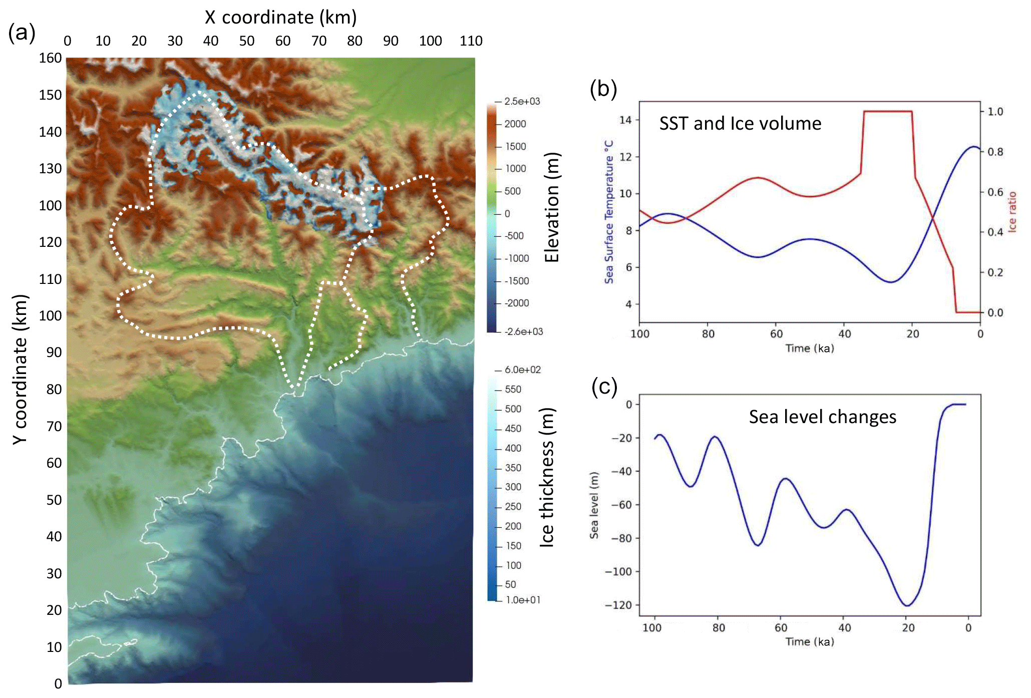
Figure 3 (a) Topography, bathymetry and maximum ice thickness (after Brisset et al., 2015) and contour of the main catchments (dashed line); (b) smoothed variations in the sea surface temperature (SST; after Hayes et al., 2015, and Rodrigo-Gamiz et al., 2013) in blue and ice thickness ratio (1 is for full ice, 0 for no ice) in red; (c) sea level variations (after Waelbroeck et al., 2002).

3.3 ¹⁰Be production and transport

¹⁰Be production rates by neutron spallation and muon capture are the same as in Mariotti et al. (2019) and computed according to Braucher et al. (2011) and Martin et al. (2017) for a latitude of 40^∘ (Table 1) using the scaling parameters by Stone (2000). Earth magnetic field variations are not considered in this study. The topographic shielding is computed from the TIN topographic grid. A shielding correction can be applied to account for the topographic smoothing due to the digital elevation model (DEM) resolution, which tends to underestimate the actual shielding (Norton and Vanacker, 2009).

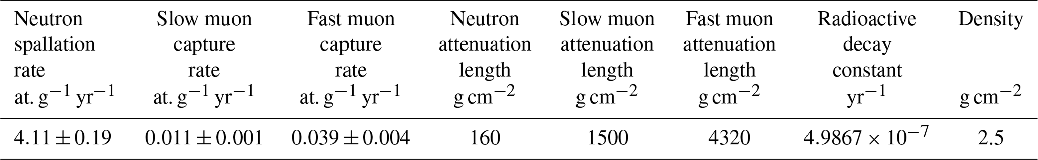
Table 1 Sea level high-latitude parameters for ¹⁰Be production (after Braucher et al., 2011).

A map of quartz-bearing rocks is defined according to the geological map of Nice and its hinterland in Rouire et al. (1980); most quartz-bearing rocks correspond either to granitic and metamorphic Palaeozoic basement rocks in the Mercantour massif or to Cenozoic sandstones in the sedimentary cover (Fig. 1). The average quartz concentration in source rocks is fixed at 50 %. The initial ¹⁰Be concentration in quartz-bearing rocks is computed assuming a steady-state average denudation rate for the whole grid. ¹⁰Be concentration N(z,t) varies with time and depth, and we simply compute it at the surface (z=0) of eroded domains (Lal, 1991):

$$\begin{array}{}\text{(8)}& {\displaystyle \frac{\mathrm{d}N(\mathrm{0},t)}{\mathrm{d}t}}=P(\mathrm{0},t)-\left(\mathit{\lambda }+{\displaystyle \frac{\mathit{\rho }\cdot \mathit{\epsilon }\left(t\right)}{\mathrm{\Lambda }}}\right)N(\mathrm{0},t),\end{array}$$

where N is the ¹⁰Be concentration (at. g⁻¹), P is the production rate (at. g⁻¹ yr⁻¹), λ is the ¹⁰Be radioactive decay constant (yr⁻¹), ρ is the rock density (g cm⁻³), Λ is the attenuation length (g cm⁻²) and ε is the erosion rate (cm yr⁻¹). At each time step, the production rate is computed taking into account the quartz abundance of the source rock and the potential shielding of cosmic rays by the surrounding topography and/or by the ice or sea cover.

¹⁰Be production results primarily from neutron spallation and fast and slow muon capture with different production rates and attenuation lengths (Braucher et al., 2011) (Table 1). Assuming that erosion and production rates are constant during a given time step of the model, we can explicitly compute the ¹⁰Be concentration in each eroded node of the source rocks at each time step, without any a priori steady-state assumption (Knudsen et al., 2019):

$$\begin{array}{}\text{(9)}& \begin{array}{rl}N(\mathrm{0},t)& =N(\mathrm{0},t-\mathrm{\Delta }t)\cdot \exp \left[-\left(\mathit{\lambda }+{\displaystyle \frac{\mathit{\rho }\cdot \mathit{\epsilon }\left(t\right)}{\mathrm{\Lambda }}}\right)\mathrm{\Delta }t\right]\\ & +{\displaystyle \frac{P(\mathrm{0},t)}{\mathit{\lambda }+\frac{\mathit{\rho }\mathit{\epsilon }\left(t\right)}{\mathrm{\Lambda }}}}\cdot \left(\mathrm{1}-\exp \left[-\left(\mathit{\lambda }+{\displaystyle \frac{\mathit{\rho }\mathit{\epsilon }\left(t\right)}{\mathrm{\Lambda }}}\right)\mathrm{\Delta }t\right]\right).\end{array}\end{array}$$

This Eulerian formulation, where the erosion rate ε is equal to the vertical velocity at which the rock material is vertically advected up to the surface is chosen because it does not necessitate computing vertical concentration profiles for each grid point.

For the initial ¹⁰Be concentration N(0, 0) we assume a steady state between ¹⁰Be production and erosion by imposing a mean long-term erosion rate ε₀:

$$\begin{array}{}\text{(10)}& N(\mathrm{0},\mathrm{0})={\displaystyle \frac{P(\mathrm{0},\mathrm{0})}{\frac{\mathit{\rho }\cdot {\mathit{\epsilon }}_{\mathrm{0}}}{\mathrm{\Lambda }}+\mathit{\lambda }}}.\end{array}$$

At each time step, the total sediment, quartz and ¹⁰Be fluxes are computed on each grid node. In the case of deposited sediments, we then compute the mean detrital ¹⁰Be concentration and quartz content of sediments, knowing the volume contribution, quartz proportion and ¹⁰Be concentration of each eroded source to the total amount of deposited sediments, assuming a perfect mixing between all sources. As initial conditions, we use a smoothed topographic and bathymetric DEM with a spatial resolution of 500 m × 500 m.

In a first test, a simulation is run with a constant precipitation rate of 0.5 m yr⁻¹ over 5000 years with a time step of 100 years in order to calibrate SPL parameters, mainly the erodibility coefficient K against the results of Mariotti et al. (2019). From this model (M1), we compute the ¹⁰Be production rate in the Mercantour massif, the mean ¹⁰Be concentration of continental river sediments corresponding to the catchments sampled by Mariotti et al. (2019) and the related mean catchment denudation rate deduced from these concentrations with an initial steady state ¹⁰Be concentration computed using a mean denudation rate of 0.2 mm yr⁻¹, in agreement with Mariotti et al. (2019) (Fig. 4 and Table 2). Discrepancies between our model and the results of Mariotti et al. (2019) can arise from (1) the fact that we use a smoother topographic grid and a simpler map of quartz-bearing areas (for ¹⁰Be production rate mismatches) and (2) the fact that we compute erosion for each grid node and then average it over the catchment area instead of considering a spatially homogeneous catchment denudation rate (for erosion rate mismatches). Data from the Coulomp River, a small tributary of the Var River, could not be satisfyingly reproduced (Table 2, Cou-16.1): the predicted low ¹⁰Be concentration resulted in a denudation rate more than twice that of Mariotti et al. (2019). Similarly, one point in the Vésubie River (Ves-16.1), which has a large ¹⁰Be production rate, shows a modelled ¹⁰Be concentration slightly larger than measured by Mariotti et al. (2019). As a consequence, the erosion rate for this point is underestimated (Fig. 4). While not perfect, simulated estimates of ¹⁰Be production and erosion rates provide a good fit with observations and allow us to constrain the value of K. Several improvements might reduce the observed discrepancies, first by using a higher DEM resolution and second by accounting for underground (karstic) water circulation known to take place in the region, like for the Coulomp River (Audra et al., 2009), which should modify river discharge and related incision rates.

Table 2 Calibration of ¹⁰Be production and erosion rates after the results of Mariotti et al. (2019) for the present-day rates.

Table 3 Model parameters.

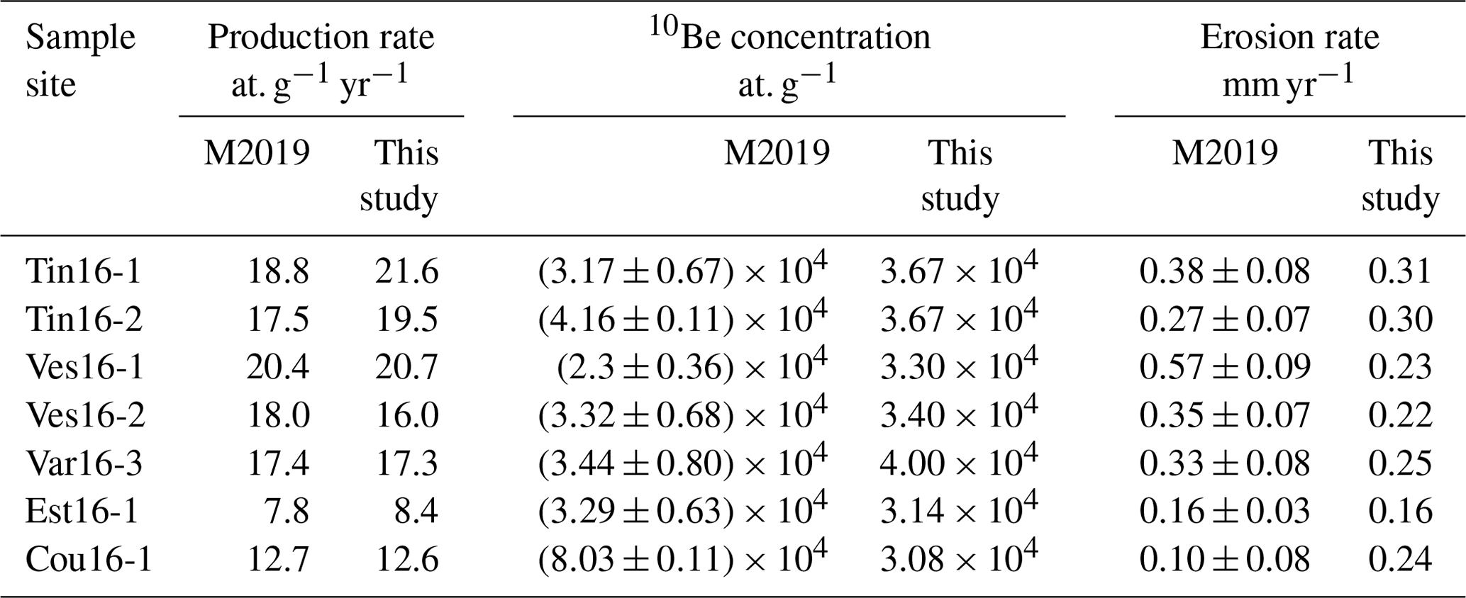
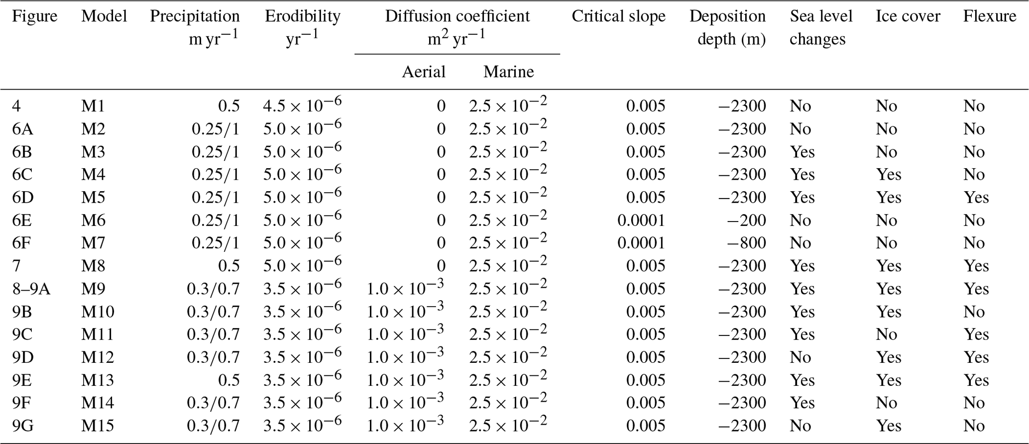
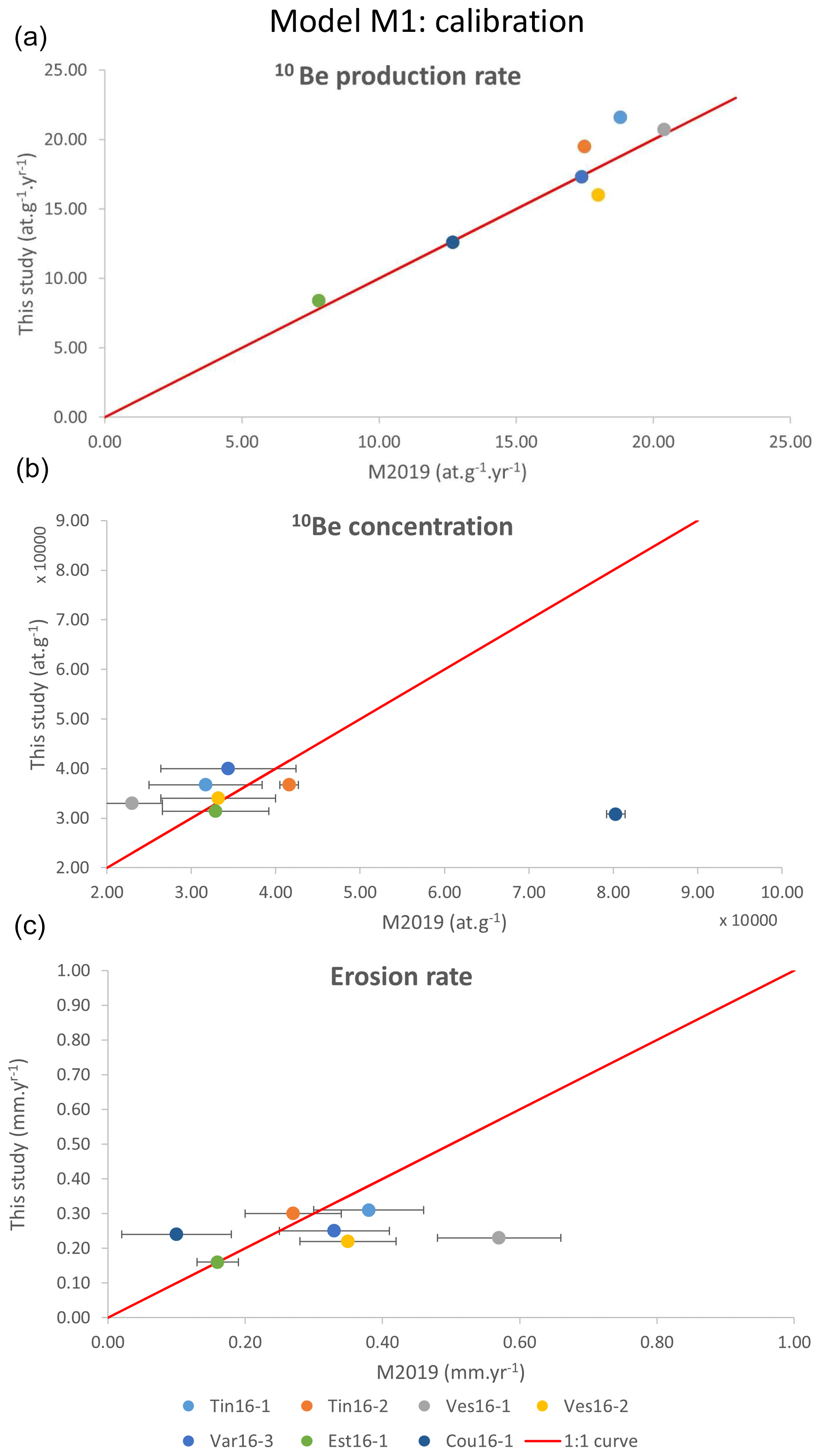
Figure 4 Comparison between the results of Mariotti et al. (2019) (x axis) and the short-term model (this study, y axis) for several rivers of the Var catchment for ¹⁰Be production rates (a), ¹⁰Be concentration in river sediments (b) and steady-state erosion rates (c). Red line indicates the 1:1 slope. See Table 2 for values.

4 Results

4.1 Record of time-variable erosion rates in river sands and at sea

We then test the response of a topographic grid representing the Var aerial and submarine systems to climatic (precipitation) variations. The model runs for 100 kyr with an adaptive time step of a maximum of 1000 years. We keep a constant rock erodibility of $\mathrm{5}\times {\mathrm{10}}^{-\mathrm{6}}$ yr⁻¹ and a hillslope diffusion coefficient of $\mathrm{2.5}\times {\mathrm{10}}^{-\mathrm{2}}$ m² yr⁻¹. The river sediment load is computed from water discharge using rating parameters (Syvitski et al., 2000) a and b  for the Var River equal to $\mathrm{1}\times {\mathrm{10}}^{-\mathrm{3}}$ and 1.6, respectively, and a low-threshold flow density (equal to water density), which ensures that all river sediments are exported to the deep submarine basin and that no large river delta is formed near the coastline.

In a first series of tests, we want to investigate how well the ¹⁰Be concentrations in continental (i.e. in river sand) and submarine (turbidite-like) deposits compare with the average catchment denudation rate directly output by the model. For this purpose, we select the total area of the Var catchment where ¹⁰Be is produced and compute the average ¹⁰Be concentration N_ex in the volume of rock eroded from this source for each time step (hereafter called “in situ” sediments because they are not yet transported or deposited) from the contribution of each catchment node i, such that

$$\begin{array}{}\text{(11)}& \stackrel{\mathrm{‾}}{N_{\mathrm{ex}}}={\displaystyle \frac{\sum _{i=\mathrm{1}}^n{N}_i{\mathit{\epsilon }}_i{Q}_i}{\sum _{i=\mathrm{1}}^n{\mathit{\epsilon }}_i{Q}_i}},\end{array}$$

where Q_i is the quartz abundance, N_i is the ¹⁰Be concentration (at. g⁻¹) and ε_i the eroded mass of sediments (in g). Then we use Eq. (10) to compute the catchment denudation rate assuming a steady-state condition and compare it with the average “actual” denudation rate directly output by the model (i.e. the average volume of eroded sediments in the same area per time step). Finally, we extract the average ¹⁰Be_MS value in an $\sim \mathrm{8}\times \mathrm{8}$ km square areas located at the mouth of the Var River for model M6, in the submarine canyon for model M7 and in the deep submarine basin for models M2 to M5. We then use the same equation to compute the average catchment denudation rate as recorded by deep-sea sediments (as shown in Fig. 5). Simulations are run with alternating low (0.25 m yr⁻¹) and high (1 m yr⁻¹) precipitation rate periods lasting 20 kyr each (Fig. 6). The first simulation (M2) is run with a constant sea level, no ice cover and no lithospheric flexure; then we successively implement a variable Mediterranean sea level, ice cover in the Mercantour massif (M3 and M4; see Fig. 3) and lithospheric flexure with a constant EET of 20 km (M5), which corresponds to a moderately rigid lithosphere where the crust and mantle elastic lids are decoupled (Burov and Diament, 1995). The last two models of this series (M6 and M7) have similar parameters to M2 except that (i) we drastically decrease the slope threshold for alluvial plain deposition, which almost impedes sediment storage on land, and (ii) we force deposition in the submarine domain at shallower depths: either in the coastal delta (−200 m) for M6 or in the submarine canyon (−800 m) for M7.

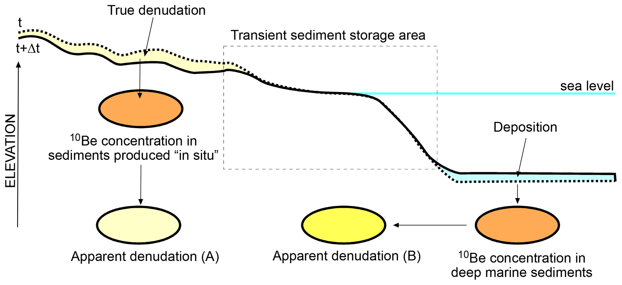
Figure 5 Schematic description of the approach used to compare the apparent denudation for a given time step computed from the mean ¹⁰Be concentration of sediments produced in situ (left part of the topographic profile, apparent denudation A) and from the mean ¹⁰Be concentration of marine sediments (¹⁰Be_MS; right part of the profile, apparent denudation B) with the true denudation.

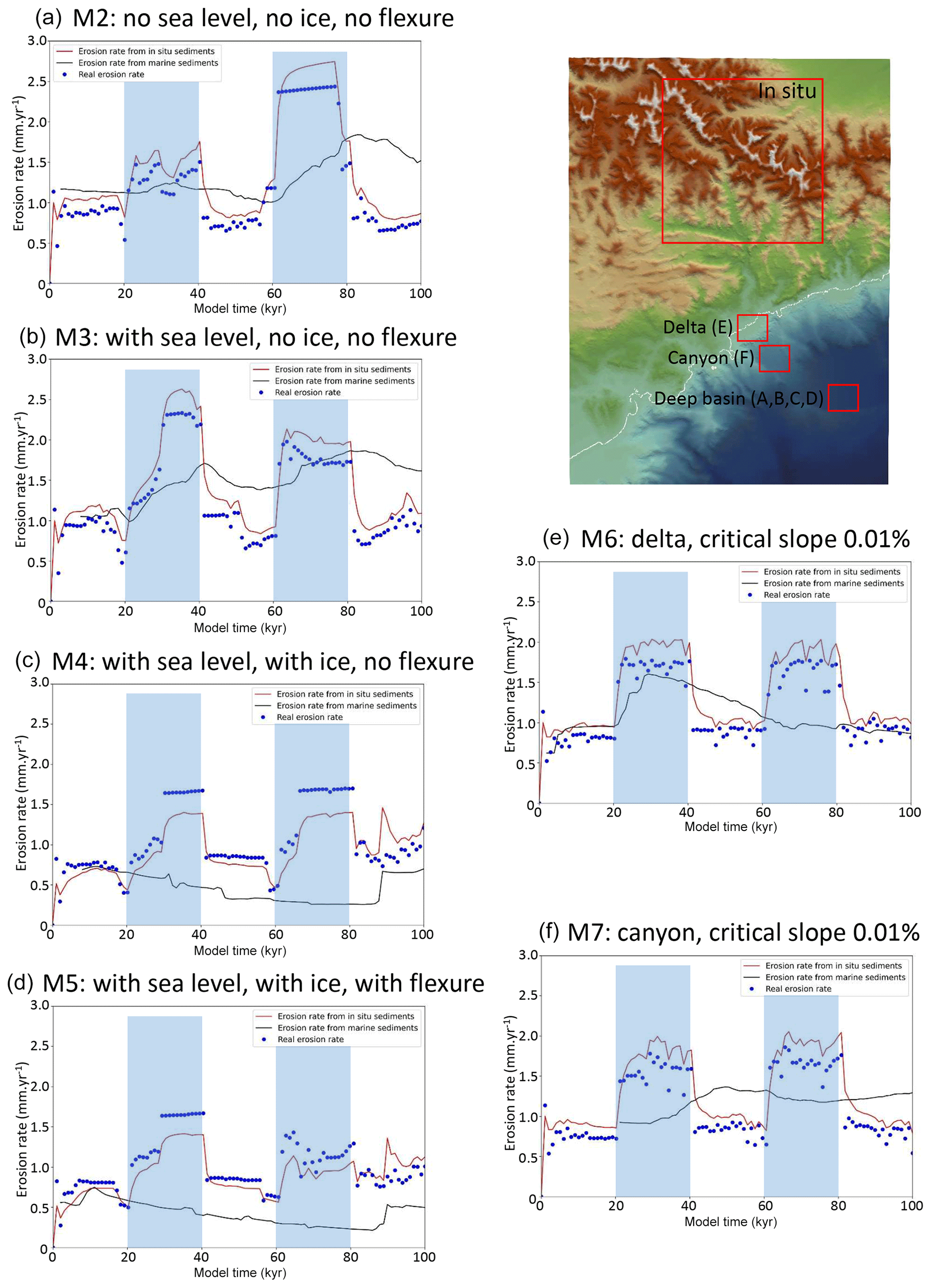
Figure 6 Test of the apparent denudation rates given by the ¹⁰Be concentration of in situ (red line) and deep marine (¹⁰Be_MS, black line) sediments versus the actual one extracted from the model (blue dots). Periods of large precipitation rates are indicated by the transparent blue vertical strips. (a) Model with only variable precipitation rate; (b) model with variable precipitation rate and sea level variations; (c) model with variable precipitation rate, ice cover and sea level variations; (d) model with variable precipitation rate, sea level variations, ice cover and flexure; (e) model similar to (a) but with a lower critical slope for sediment deposition and forced deposition below −200 m; (f) model similar to (e) but with forced deposition below −800 m.

The first model (M2, Fig. 6a), where there are no sea level changes, no ice cover and no flexural isostatic response of the lithosphere, shows that the two periods of more intense precipitation are well-detected in in situ sediments, the ¹⁰Be signature of which gives erosion rates consistent with the actual ones. Marine sediments also seem to record two periods of larger erosion rates, but the first one (between 25 and 45 kyr) is barely visible and the peak of the second one (80–90 kyr) occurs 10 to 20 kyr after the middle of the second high-precipitation period. The second model (M3, Fig. 6b), where sea level variations are present, displays approximately the same behaviour as M2 for in situ sediments, with apparent erosion rates consistent with real ones. Erosion rates computed from marine sediments also show fluctuations consistent with two periods of more intense precipitation, but they appear much smoother and offset by ∼20 kyr, compared to the actual ones. In the two following models where ice cover is present (M4 and M5, Fig. 6c and d), the effect of partial coverage of the Mercantour massif by ice during almost all the duration of the model is twofold: (i) it reduces the effect of precipitation variations, since no run-off occurs beneath the ice cover, and (ii) it reduces the production and exportation of ¹⁰Be-poor sediments, except during the last period (80–100 kyr into the model run) when the massif is free of ice. As a consequence, while in situ sediments still record the actual erosion rate well, the ¹⁰Be signal in the submarine domain strongly underestimates it. Finally, models similar to M2 but with a lower critical slope and where sediment deposition is forced either in the delta (M6) or in the submarine canyon (M7) show that marine sediments of the delta record the onset of first precipitation pulse well, with only a small time lag (5 kyr). Then, the apparent erosion rate computed from marine sediments progressively decreases, and the second period of intense precipitation is not recorded. In this model, ¹⁰Be-poor sediments coming from the second precipitation pulse are not deposited in the sampled area but further south, due to delta progradation. Finally, if deposition is forced to occur in the middle of the submarine slope, the first precipitation peak is still detected, but it appears smoother and of a lower amplitude and it occurs ∼20 kyr later than on land (Fig. 6f).

In simulations without ice cover (Fig. 6a, b, e and f), denudation rates estimated from in situ sediments do record the succession of periodic pulses but generally overestimate the actual denudation rate by a few percent. This overestimation reflects a more intense erosion in low-altitude river thalwegs than on the hillslopes and high-altitude interfluves, which slightly promotes the export of ¹⁰Be-poor sediments with respect to ¹⁰Be-rich ones, hence increasing the apparent denudation rate.

For all simulations, both in situ and actual denudation rate evolutions depict more complex patterns than the imposed climatic (precipitation) forcing. Short-period, low-amplitude variations are visible, which are related to local and internal adjustments of the modelled topography and not to the external forcing, although sea level variations seem to slightly modify their amplitude (Fig. 6a and b). There is no clear time lag between the onset of higher-precipitation periods and their record in in situ sediments, but the apparent denudation rate from in situ river sediments displays a curved shape at the transition between low- and high-precipitation rate periods (well visible, for instance, in Fig. 6a between 60 and 80 kyr of the model run), which corresponds to well-known analytical solutions for periodic changes in erosion rates (Bierman and Steig, 1996) and is consistent with the detachment-limited hypothesis. This reflects the time needed for ¹⁰Be concentration to reach a steady state relative to the massif denudation rate (∼5 kyr); this effect is also visible at the transition from high to low precipitation rates (Fig. 6e and f).

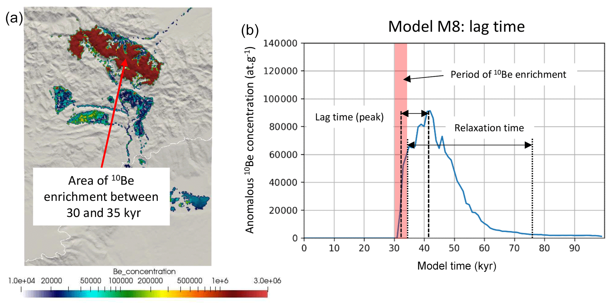
Figure 7 Difference in ¹⁰Be_MS between two models with the same parameters (Table 3), one of them having imposed ¹⁰Be-rich (2×10⁶ at. g⁻¹) rocks above 1800 m between 30 and 35 kyr (transparent red vertical strip in panel b). Panel (a) shows the location of the area of ¹⁰Be enrichment in the Mercantour massif. The time lag (thick dashes) is defined as the interval between the middle of the ¹⁰Be enrichment period in the massif and the age of the largest ¹⁰Be peak in marine sediments. The relaxation time is defined as the interval between the end of the ¹⁰Be enrichment period in the massif and the end of excess ¹⁰Be recorded in marine sediments.

This series of tests seem to indicate that (i) the alluvial sediments produced in situ record the variations in the rate of denudation well, although they may slightly overestimate them; (ii) ¹⁰Be of submarine sediments ¹⁰Be_MS in the deepest part of the basin does not allow us to retrieve sharp climate variations, especially if glaciers cover the area where ¹⁰Be is produced for a long period of time, but correctly estimate the average long-term erosion rate, with only smooth variations; and (iii) finally, there can be a significant time lag between the middle of the high-precipitation periods and the peak in denudation rates recorded in submarine sediments.

In order to refine our understanding of the smoothing and time lag effects, we aimed at tracing artificially enriched ¹⁰Be-rich sediments in the mountain range down to the submarine basin. To do so, we imposed a constant and artificial high ¹⁰Be concentration in high-altitude areas (above 1800 m) over a 5 kyr period from 30 to 35 kyr into the model run. Then, we compare the ¹⁰Be signature of deep-sea sediments between two identical models: one run with the ¹⁰Be enrichment and one without (model M8, Fig. 7). We do not show all the tests here for the sake of simplicity but rather illustrate a typical signature of this transient ¹⁰Be enrichment as visible in submarine sediments. This result is obtained accounting for a variable sea level, ice cover and lithospheric flexure and a constant precipitation rate of 0.5 m yr⁻¹ (Table 3). If we consider the earliest arrival of ¹⁰Be-rich sediments in the submarine basin, the time lag from source to sink appears to be relatively small (1–3 kyr) since ¹⁰Be-rich sediments arrive in the basin shortly after they begin to be produced in the massif (Fig. 7); however, the time lag between the middle of the ¹⁰Be enrichment period on land and the largest ¹⁰Be peak recorded in marine sediments is rather large (∼10 kyr). Moreover, this signal takes a long time to relax: sediments that are richer in ¹⁰Be than the reference simulation still reach the basin ∼25 kyr after the end of the enrichment period. These tests suggest that, although the initial time lag is not necessarily very important, the relaxation time, i.e. the time it takes for the ¹⁰Be concentration to return to its background value, can be large. It suggests that, in the case of a succession of climatic events with a frequency greater than this relaxation time, it will therefore be impossible to differentiate between them in the ¹⁰Be signal. We want to stress here that this delay is different from the time needed to reach cosmogenic radionuclide steady state, as computed in Bierman and Steig (1996). Here, we do not force high ¹⁰Be concentration in the Mercantour massif by drastically reducing the erosion rate; it would indeed take some time for the ¹⁰Be signal to adapt and reach a new steady state. Instead, we instantaneously apply a large, artificial ¹⁰Be value in the mountain peaks, which should be immediately visible in deposited sediments if the time lag was zero.

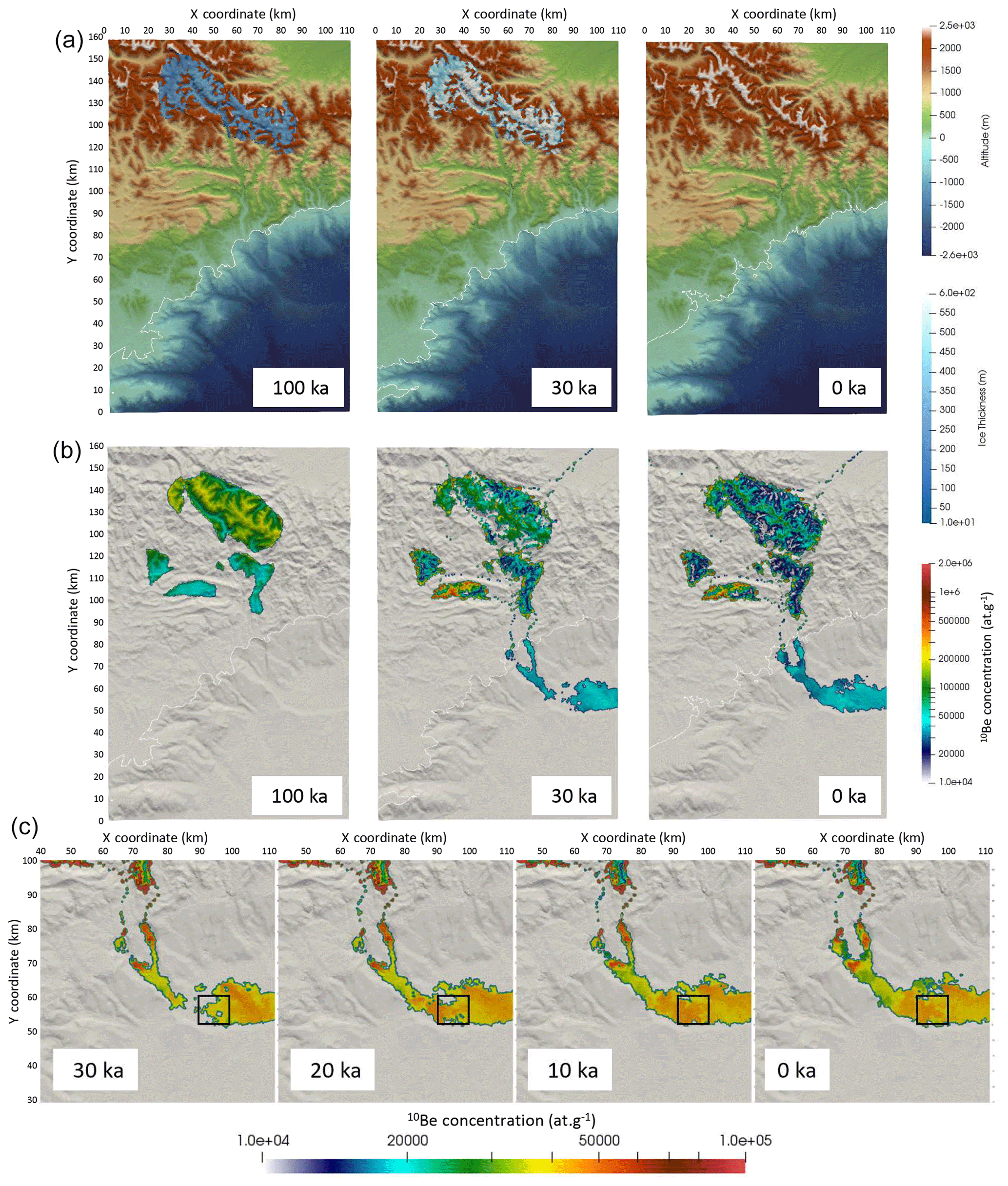
Figure 8 Stages of evolution of the reference model from 0 to 100 kyr (model time counted forward, corresponding to 100 to 0 ka in reality and on the figure time stamps). Upper panels (a) present the topography and ice thickness, middle panels (b) present the surface ¹⁰Be concentration and lower panels (c) present a blow-up of the surface ¹⁰Be concentration in submarine sediments in the last 30 kyr, with an adjusted colour map. The solid rectangle in the lower panels indicates the area where average ¹⁰Be_MS has been computed (see results in Fig. 9).

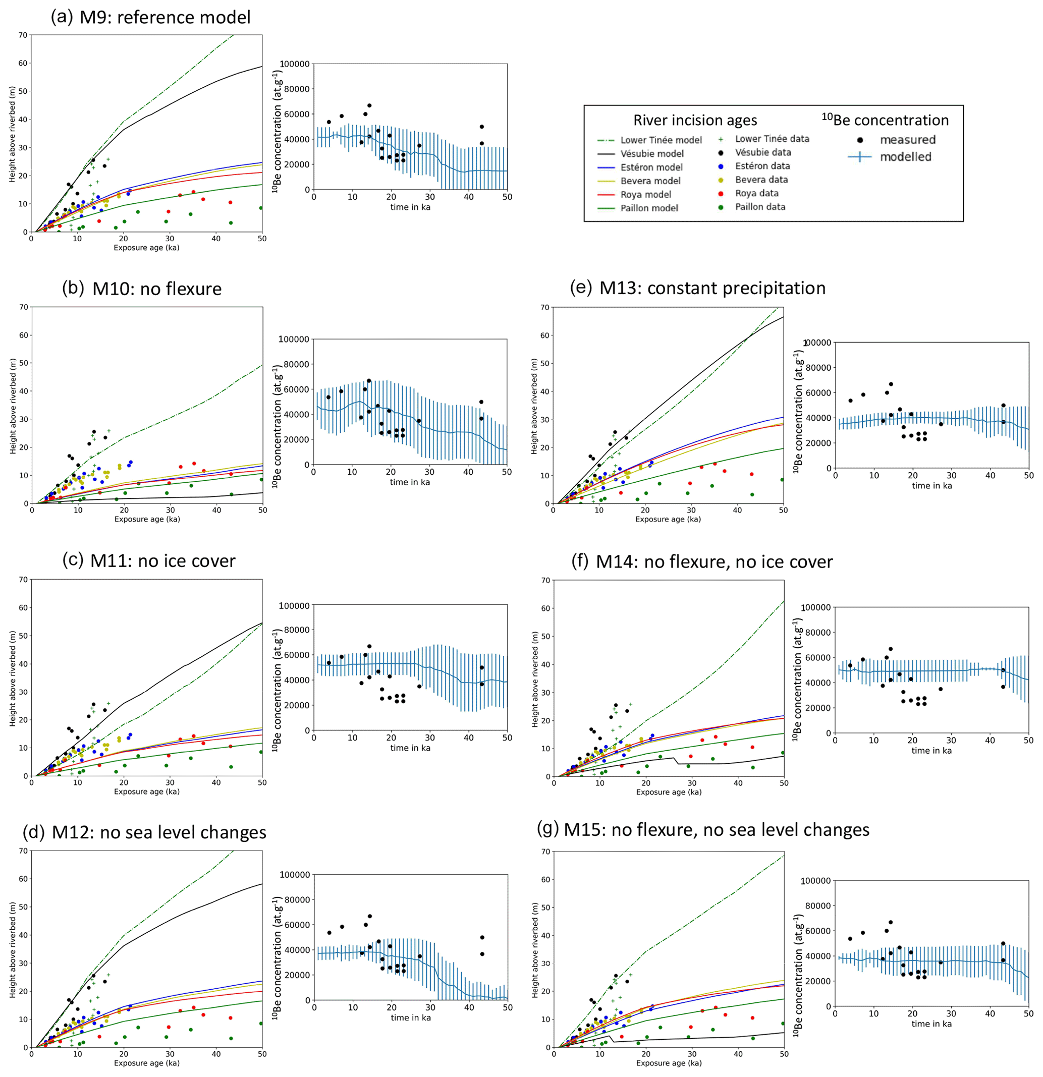
Figure 9 Comparison between model outputs and data from CRE ages in river-polished cliffs (a–d; see Fig. 2) and ¹⁰Be_MS (e–g; after Mariotti et al., 2021). Vertical bars in the right-hand graphs of each panel correspond to measured standard deviations in ¹⁰Be_MS in the sampled area (Fig. 8). See Table 3 for model parameters.

4.2 Reference model for the Var catchment over the last 100 kyr

Finally, we try to determine if it is possible to find model parameters for which the result matches both the previously determined river incision rates during the last 30–40 kyr in the Nice hinterland (Fig. 2) and measured ¹⁰Be_MS for the same period (Mariotti et al., 2021). We chose not to consider the two river gorge sites that have been dated in the upper Tinée valley (Salso Moreno and Isola; see Fig. 1) because they likely correspond to very transient post-glacial sediment wash-out that it is not possible to model (Rolland et al., 2020). This “reference” model has been determined by a trial-and-error method, with initial and boundary conditions similar to the previous series of runs (Figs. 8 and 9a, model M9). Sea level variations and ice cover are imposed, and simulations are run for 100 kyr with a time step of 1 kyr. We assume that for the last period of the model, which corresponds to the present-day situation, the precipitation rate should be compatible with current average values (i.e. 700–800 mm yr⁻¹; https://meteofrance.com/climat/normales/france/provence-alpes-cote-d-azur/NICE, last access: 25 February 2023). Here again, the flexural isostatic response is computed using a constant effective elastic thickness of 20 km. We also tested different EET values of 10 and 30 km as well as a space-variable EET, with larger values on land than at sea. Since variations in EET are difficult to constrain and only cause minor differences in the final result, we chose to impose this constant value of 20 km on the entire grid for all models. We first present a model which satisfyingly reproduces measured river incision rates and ¹⁰Be measurements; then we discuss the implications of each parameter (flexure, sea level, ice cover) in the final result. This simulation involves a precipitation rate of 0.3 m yr⁻¹ from 0 to 80 ka increasing to 0.7 m yr⁻¹ during the last 20 kyr, an initial denudation rate of 0.2 mm yr⁻¹, a diffusion coefficient of $\mathrm{2.5}\times {\mathrm{10}}^{-\mathrm{2}}$ m² yr⁻¹ in submarine and river sediments and of 0.1 m² yr⁻¹ in bedrock areas, and a constant erodibility coefficient of $\mathrm{3.5}\times {\mathrm{10}}^{-\mathrm{6}}$ yr⁻¹ (Figs. 8 and 9a and Table 3). This model satisfyingly reproduces measured incision rates in river channels and yields a slight increase in ¹⁰Be_MS in the Var deep-sea fan after ∼40 ka (Fig. 9a). Given the large variability of ¹⁰Be_MS values (as depicted by the standard error bars), the modelled ¹⁰Be_MS variation is compatible with almost all measurements published in Mariotti et al. (2021).

From the simulation outputs, we find that the increase in ¹⁰Be_MS is not due to a change in erosion rate on land: indeed, river incision rates tend to increase after 20 ka due to the release of glacier meltwaters and to increased precipitation rates, while the ¹⁰Be_MS also increases 2-fold. The observed increase in ¹⁰Be_MS around 30–40 ka is partly due to the presence of patches of ¹⁰Be-rich sediments deposited in the upper part of the basin after about 30 ka, which slowly feed lower areas of the basin in ¹⁰Be-rich sediments during the run (Fig. 8b and c). The simulation fit with the measured ¹⁰Be_MS may somehow be fortuitous, since the surface concentration in ¹⁰Be varies at lot, both locally and vertically. This simulation thus shows that (1) ¹⁰Be concentration at the surface of the submarine basin at a given time can be highly variable (hence, the vertical variation in ¹⁰Be_MS can also be variable from one place to another) and that (2) it is quite possible to get both increased incision rates on land and apparent decreased denudation rates in submarine cores for the same external (climatic) forcing.

Starting from this reference simulation (Fig. 9a), we then evaluate the individual effects of lithospheric flexure, ice cover and sea level changes. A similar simulation without lithospheric flexure predicts slightly lower incision rates for all rivers, with a more dramatic change for the Vésubie River where it drastically decreases (Fig. 9b, model M10); meanwhile, both the absolute values of ¹⁰Be_MS and their variations are still consistent with measurements. A simulation similar to the reference one but without ice cover (Fig. 9c, model M11) predicts slightly too low incision rates for some rivers (Estéron, lower Tinée) but a good fit to ¹⁰Be_MS and to some other rivers (Paillon and Roya) and rather high and constant ¹⁰Be_MS. Removing sea level changes does not significantly affect the simulated river incision rates but gives a lower ¹⁰Be_MS signal, still with an increase after 30 ka (Fig. 9d, model M12). A simulation with a constant precipitation rate gives satisfying results for the river incision rates but a constant and too low ¹⁰Be_MS, especially for the most recent (20 to 0 ka) period (Fig. 9, model M13). Finally, removing both the flexural isostatic response of the lithosphere and the main sources of load (i.e. ice cover and sea level variations) has large effects both on the river incision rates (especially for the Vésubie River) and on the ¹⁰Be_MS signal (Fig. 9f and g, models M14 and M15). Interestingly, the last three models without precipitation changes or without flexure ± ice cover or sea level changes produce rather stable ¹⁰Be_MS values throughout the model. In fact, the main difference between the reference model M9 and for instance models M13, M14 and M15 is that the first 50 kyr of model M9 are characterized by a lower ¹⁰Be_MS concentration. This is possibly due to a relatively lower contribution of high-altitude rocks to the ¹⁰Be_MS signal when the massif is partly covered by ice.

Based on these models, we show the following:

• Simulations with constant precipitation or without flexure and without either ice cover or sea level changes do not produce the observed increase in ¹⁰Be_MS after 30–40 ka.

• The large incision rate in the Vésubie River (compared to Bevera, Roya, Estéron and Paillon) can only be explained by the effect of isostatic rebound, the latter being smaller in the simulations with no glaciers.

• Cosmic ray exposure (CRE) data on river-polished walls are not dense enough to discriminate between constant (0.5 mm yr⁻¹) or variable (0.3 then 0.7 mm yr⁻¹) precipitation rates.

• However, a constant precipitation induces more important denudation in the earliest stages of the predicted evolution (compared to the reference simulation where precipitation rate is low), hence producing on average a lower ¹⁰Be_MS at the end of the model.

• A combination of sea level changes, ice cover and lithospheric flexure provides a reasonable fit both to river incision rates and to measured ¹⁰Be_MS.

5 Discussion and conclusions

These series of models, where continental sediment deposition is controlled almost exclusively by one parameter (the critical slope for alluvial deposition), show that it is sufficient to induce significant differences in the ¹⁰Be signal between its production in quartz-bearing rocks of high-altitude massifs and its record in the submarine domain. However, here, we do not capture all the details of erosion, transport, sediment mixing and sedimentation, as we do not consider different lithologies, grain sizes, or any complex mixing law between the various sediment sources. In contrast to the study by Carretier et al. (2020), the lack of grain tracking prevents us from being able to measure particle residence times and compare them to the average geochemical signature of the sediments.

Submarine sediment transport and deposition modelling is almost as simple as on land and does not consider ocean dynamics (turbulence of turbiditic flows, coastal currents), which are responsible for characteristic sedimentary features such as the Var sedimentary ridge at the bottom of the Var Canyon (Migeon et al., 2001). These phenomena can also contribute to sediment dispersion and smoothing of the ¹⁰Be signal offshore.

Similarly, it could be interesting to couple our models with glacial erosion models (e.g. Seguinot and Delanay, 2021) in order to better control the variability of glacial erosion and sediment production during the last cycles and better quantify how it affects ¹⁰Be production and exportation.

Finally, initial model conditions are another possible source of uncertainty, especially when it comes to our initial topography, which is derived from present-day elevation and therefore limits our ability to run the model over a longer period of times as it would produce a final topography too different from the current one. A better estimate of initial quartz abundances in source rocks (i.e. crystalline lithologies of the Mercantour massif and Cenozoic sandstones of the foreland) would also help to reduce the uncertainties associated with quartz and ¹⁰Be transfer from source to sink.

Our results based on dating and modelling indicate that, while river sands do accurately estimate the average denudation rate of continental catchments for the Var region (provided the latter does not vary at high frequency, i.e. with periods smaller than the time needed to reach a steady state), this is much less the case for submarine deep-sea sediments. These sediments have a different and often much smoother signature than continental ones and record significant lag and/or relaxation times with respect to external forcing, probably due to the geomorphological response of the continental margin both on land and at sea. With this area being prone to strong and rapid geomorphological modifications (i.e. transition from narrow bedrock channels to wide, braided rivers) during violent flood events (like during the Storm Alex, which took place in October 2020), it could be of primordial importance to estimate the relaxation time of such events and their role in the long-term landscape evolution and geochemical signature of the sedimentary archives.

On the long-term, the presence of ice in the massifs where ¹⁰Be production occurs together with the reworking of alluvial and deltaic sediments during low sea level periods and vertical motions due to lithospheric flexure largely modify the signal coming from precipitation variations and can lead to poor estimates of the actual denudation rate variations from ¹⁰Be_MS. All these effects have been exemplified in this study of the Var catchment where the distance from source to sink is short, precipitation rates are large and the mouths of the main rivers are devoid of any large deltas. Hence, in regions with very large catchments, alluvial plains and deltas, it could be even more difficult to reconstruct past denudation rates from deep-sea sediments.

Our reference simulation highlights the complex interactions between river incision, sea level variations, ice coverage and the resulting isostatic response of the lithosphere. It seems impossible to disentangle the respective role of any of these forcings specifically, as most of them are interdependent. However, further tests (Fig. 9) show that, depending on their location, rivers have a different sensitivity to these parameters: the Estéron, Roya, Paillon and Bevera are less affected by the parametric changes applied to the reference forcing conditions; their incision rate is only significantly reduced when considering no sea level changes, ice cover or flexure (not shown here).

In contrast, the rivers with the largest incision rates (the Vésubie and, to a lesser extent, the Tinée River) are also the ones which seem more sensitive to the effect of ice cover and flexural isostatic response of the lithosphere (Fig. 9). This is possibly because a significant part of their length (20–40 km) runs over the Mercantour crystalline massif, i.e. over the area where post-glacial isostatic rebound is important. The sampling sites of these rivers being rather close to their headwaters, they are not sensitive to sea level variations. Quantification of each river sensitivity to local or regional processes like isostatic uplift, sea level changes, precipitation or ice cover, depending on the dating site location, could therefore be useful to better understand the respective importance of these external forcings on this southern Alpine margin.